Monday, August 14, 2023

Discover the Microsoft Fabric Data Wrangler

The Data Wrangler is as interesting as hidden inside Microsoft Fabric. It’s not easy to find and activate it, but it is worth the trouble.

Before digging into the Data Wrangler, let’s analyze the data features in the query environment.

Data Features in Query Environment

The new query environment, which allow us to make data exploration with visual queries and SQL queries, is available with many Power BI features:

  • Datamarts
  • lake house
  • Data Warehouse

And probably more to come if I’m not missing some of them already.

Why are we starting on the Query Environment? Because the Query Environment has some similar features to the Data Wrangler. Let’s discover them first and compare with the features on the Data Wrangler.

This example starts on a SQL Endpoint of a lake house.

  1. Create a Visual Query.

A close up of words Description automatically generated


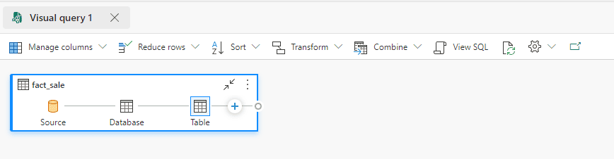
  1. Drop the table Fact_Sales to the Visual Query

A screenshot of a computer Description automatically generated

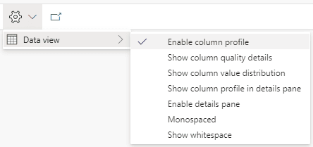
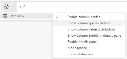
  1. On the top menu, on the Settings button, the Data View item has some interesting features for us to investigate. Let’s analyze them one by one. Description automatically generated”


"A

Enable Column Profile

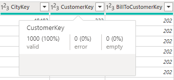
When we enable this option, a subtle green line appears on the Display Area, just below the title. If we hover this green line on a specific column, we find information about the data quality of the rows on that column.

The information tells us how many rows have valid values, error values and empty values for the column.

A screenshot of a computer program Description automatically generated


Show Column Quality Details

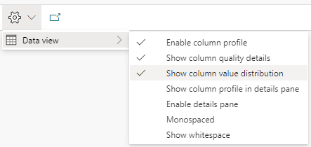
Enabling this option expands the green line. The information about data quality which was only visible when hovering a column becomes visible in the expanded panel.

A screenshot of a computer Description automatically generated


Show Value Distribution

This option adds to the panel information about the distribution of unique values in the column. It points to us how many distinct and unique values each column has.

A screenshot of a computer Description automatically generated


This information may be very useful to identify primary keys in sets of data you don’t know.


Data Wrangler

The Data Wrangler has similar information to the ones we just found on the Query Environment. However, while the query environment works in a visual environment, the data wrangler works on python notebooks.

Two additional details it worth mentioning: The Data Wrangler has more features, linked to spark notebooks and it’s difficult to locate if you don’t know exactly where to look.

Opening the Data Wrangler

The secret to opening the data wrangler is simple after you discover it: The Data Wrangler requires a Pandas data frame. Once we have a notebook opened and a Pandas dataframe loaded into a variable, the Data Wrangler becomes available.

As an example, we will use the same lake house as the previous example.

Let’s follow these steps:

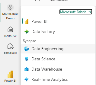
  1. Click the Experience button and select the Data Engineering experience.

A screen shot of a computer Description automatically generated


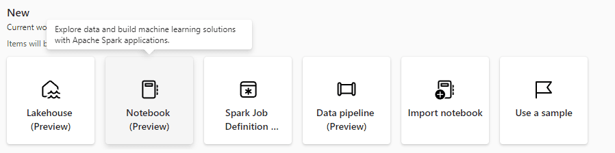
  1. Click the button New Notebook on the Data Engineering experience.

A screenshot of a computer Description automatically generated


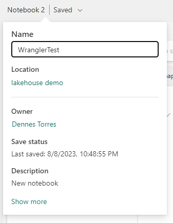
  1. On the top left, change the notebook name to WranglerTest

A screenshot of a computer Description automatically generated


  1. On the left, click the Add button to link the notebook with the lake house.

A screenshot of a computer Description automatically generated


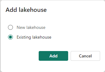
  1. On the Add lakehouse window, select the Existing lakehouse option.

A screenshot of a computer Description automatically generated


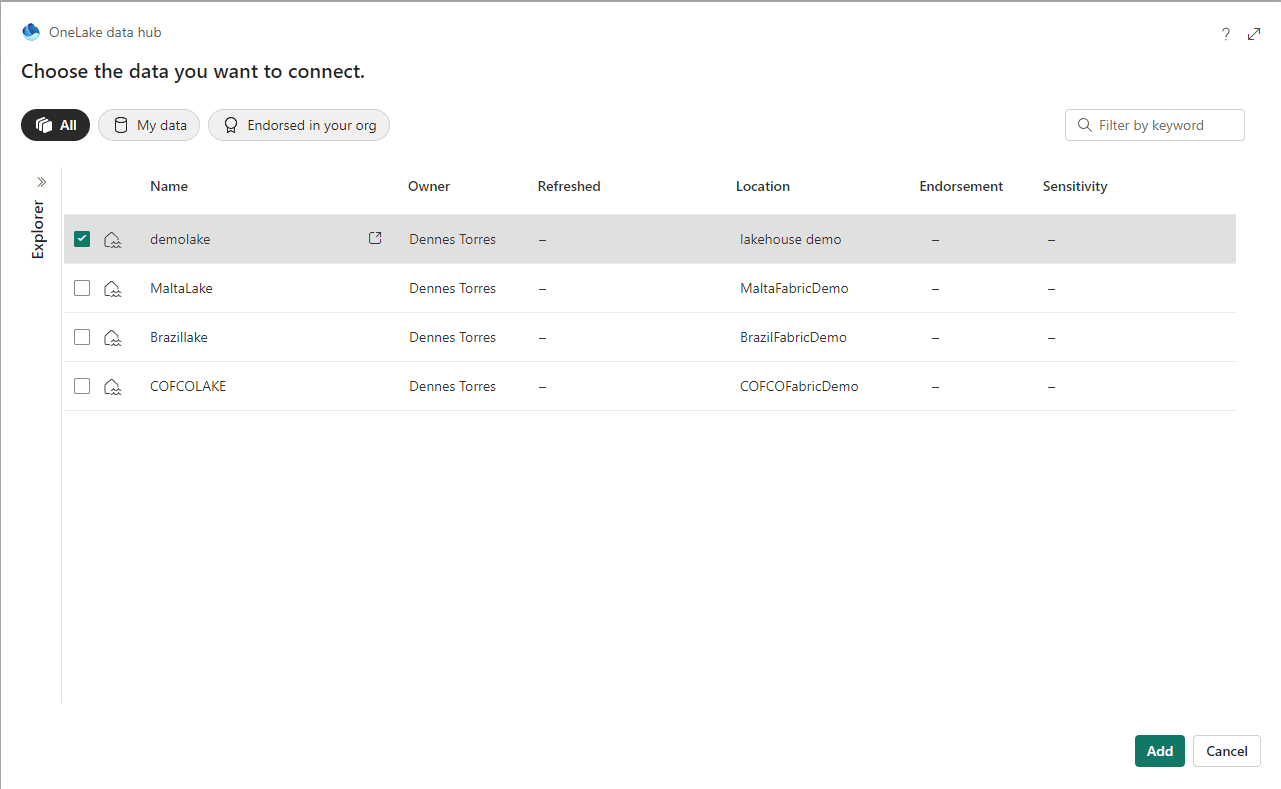
  1. Choose your lakehouse and click the Add button.

A screenshot of a computer Description automatically generated


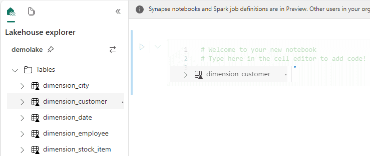
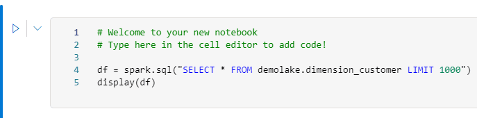
  1. Drag and drop the dimension_customer table to the code block in the notebook.

The code to load the table is automatically created. Did you know this one?

A screenshot of a computer Description automatically generated


A screenshot of a computer program Description automatically generated


  1. Remove the Display line in the code. It’s not needed.
  2. Add toPandas() at the end of Spark.sql

A screenshot of a computer Description automatically generated


  1. Execute the code block.

We will receive an error message and it explains the problem. Pandas, in the lake house environment, always try to make an optimization called Arrow optimization by default. This optimization may not work well with some fields, so we need to disable it.


  • Add the following line to the start of the code:

spark.conf.set('spark.sql.execution.arrow.pyspark.enabled', 'false')
  1. Run the code block again.

The Arrow optimization is disabled but the datetime field still causes problems. To make it easier, let’s remove the datetime field from the query.


  1. Change the SQL query in the code to the following:
SELECT customerkey,
       wwicustomerid,
       billtocustomer,
       category,
       buyinggroup,
       primarycontact,
       postalcode
FROM   demolake.dimension_customer
LIMIT  1000 
  1. Execute the code block again.

A white card with black text Description automatically generated


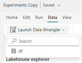
  1. On the top menu, click Data menu item.
  2. Click the Launch Data Wrangler button.

The variable created on the code block is identified and appears on the menu.

A screenshot of a computer Description automatically generated


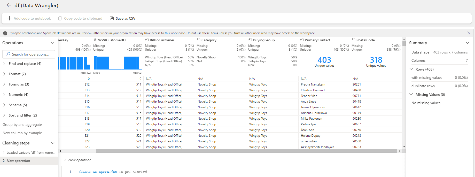
  1. Click the variable name on the menu. The Data Wrangler will appear.

A screenshot of a computer Description automatically generated


Data Wrangler: First Impressions

The initial Data Wrangler window seems like the information we have in the query environment. It seems to have some additional details about the data distribution, in some cases, making it more visible when there are only a few unique values.


If your purpose is only to see this additional information about the columns, both Data Wrangler and the query environment, work. It becomes a matter of preference which one you should use and for sure you will choose according to your preferred environment: If you prefer to work visually, the query environment will be better, if you prefer to work with spark, Data Wrangler will be better.

However, Data Wrangler can achieve much more. It can accept transformations over the data frame and implement these transformations as pyspark code.

In fact, the UI is slightly like Power Query.


Transformations with Data Wrangler

Let’s implement some transformations over the data frame and check the result.

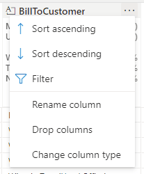
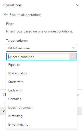
  1. Click the Expand button (“…”) beside the BillToCustomer field.

A screenshot of a computer Description automatically generated


  1. Select the Filter option on the menu.
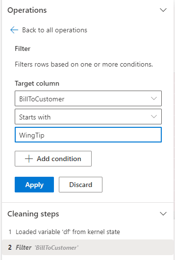
  2. On the left side, on the dropdown Select a Condition, select the option Starts With

A screenshot of a computer screen Description automatically generated


  1. On the 3rd textbox, type WingTip

A screenshot of a computer Description automatically generated


  1. Click the Apply button.

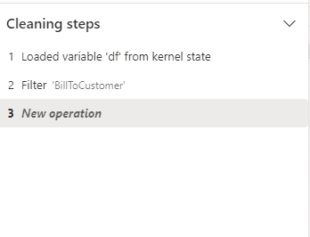
Mind the Cleaning steps, registering the transformations.

A screenshot of a computer Description automatically generated


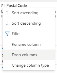
  1. Click the Expand button (“…”) beside the PostalCode field.
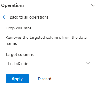
  2. Select the Drop Columns option on the menu.

A screenshot of a computer Description automatically generated


  1. Click the Apply button.

A screenshot of a computer Description automatically generated

  1. On the top menu, click the Add code to notebook button.

A screenshot of a computer Description automatically generated


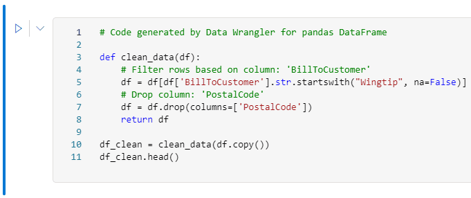
The transformations created visually are included in the notebook as part of the code.

A screenshot of a computer code Description automatically generated


Summary

The Data Wrangler is a powerful tool not only to help data exploration but also to help building pyspark code using visual methods.


The post Discover the Microsoft Fabric Data Wrangler appeared first on Simple Talk.


from Simple Talk https://ift.tt/1T9EvA3
via

Working around schema drift in SQL Server

At Stack Overflow, our environment has multiple implementations of a largely – but not 100% – identical schema. (By “schema,” I mostly mean the set of tables within a database.) I sometimes need to retrieve or update data across a large number of sites. Let’s say, pulling or removing information from the Users table, and related tables, across all of our databases.

This gets complicated.

Because:

  • Each of our Q & A sites has its own database, and each database has a table called Users (and some metadata is split out into a separate UserMetadata table).
  • A few sites are special, like Area 51, where the Users table looks a little different (it is wider, because the UserMetadata split isn’t present here for historical reasons).
  • A few others look like Q & A databases, like Chat. They also contain a table called Users, but here the table is used differently and the column structure is unique.
  • Stack Overflow for Teams is more complex. A team’s tables are shared with others within a single database, with the boundary being a schema instead of a database. There is no table called dbo.Users, but a database may contain multiple Users tables, such as Team0001.Users, Team0002.Users, and so on. I’ll deal with this special case in a future post.

IntelliSense highlights a few of these differences straight away:

IntelliSense reveals schema drift

Schema has “drifted” in these and other cases, for example when features are only applicable to one site, team, or product. Features like Collectives, Saves, or Staging Ground can lead to new columns or even entire tables that are only present in some databases.

This is okay, and there are many ways to deal with drift – even drift by design. But that’s not the point of this post. Because even if I could convince everyone all of our databases should have identical schema, I can’t snap my fingers and make it happen overnight. In the meantime, I have to deal with these differences.

A fake example.

Imagine I want to collect a list of users with more than one answer and who mention groundhogs in the “About Me” section of their profile. In any Q & A database, I can issue the following query:

SELECT u.Id, u.AnswerCount
   FROM Users AS u
   INNER JOIN UserMetadata AS um
   ON u.Id = um.UserId
   WHERE um.AboutMe LIKE N'%groundhogs%'
   AND u.AnswerCount > 1;

That works fine across “normal” site databases.

But there are exceptions.

In the Area 51 database, that query fails. As mentioned above, there is no UserMetadata table, and AnswerCount is not aggregated anywhere. I have to write the query differently:

SELECT u.Id, AnswerCount = COUNT(p.Id)
   FROM Users AS u
   INNER JOIN Posts AS p
   ON u.Id = p.OwnerUserId
   AND p.PostTypeId = 2
   WHERE u.AboutMe LIKE N'%groundhogs%'
   GROUP BY u.Id
   HAVING COUNT(p.Id > 1);

In the Chat database, this query makes no sense, because there are no answers. So I want an easy way for this database to be skipped entirely.

The problem.

I don’t want to hard-code lists of databases that happen to support one version of the schema or another right now. This reminds me of browser detection techniques that rely on the user agent string the browser presents, rather than testing the required functionality. Picture maintaining a list of all possible user agent strings and keeping it up to date. This is simply unmanageable, and I don’t want to do it for database names, either. I want it to be dynamic, so I don’t have to update some list somewhere every time a new database gets added, existing schema drift gets corrected, or new schema drift appears. And sometimes new schema drift will appear, like with new features, as mentioned before. We know about this drift; it goes through PRs and reviews, and is what I call controlled drift. The technique I use relies on knowing the schemas are well controlled, and being aware of changes coming out. So if someone goes rogue and creates a new table in Area51 called dbo.MoreUserMetadata, and starts stuffing information about groundhogs in a random column there without anyone’s knowledge, that data will go unnoticed. That is one caveat to the solution I’ll propose.

A piece of the puzzle.

I have to repeat this process for a growing list of queries. So, in our central DBA database, I have an Actions table that I use to validate the metadata in each database before attempting to run a given query there.

USE DBA;
 GO

 CREATE TABLE dbo.Actions
 (
   ActionID     int,
   QueryText    nvarchar(max),
   CheckTable1  nvarchar(128),
   CheckColumn1 nvarchar(128),
   CheckTable2  nvarchar(128),
   CheckColumn2 nvarchar(128)
 );

I put these queries into the table (minus the statement terminator, since these will later be placed inside a common table expression):

INSERT dbo.Actions
 (
   ActionID,    QueryText, 
   CheckTable1, CheckColumn1, 
   CheckTable2, CheckColumn2
 )
 VALUES
 
   (1, N'SELECT u.Id, u.AnswerCount
         FROM Users AS u
         INNER JOIN UserMetadata AS um
         ON u.Id = um.UserId
         WHERE um.AboutMe LIKE N''%groundhogs%''
         AND u.AnswerCount > 1',
       N'Users',        N'AnswerCount',
       N'UserMetadata', N'AboutMe'),

   (2, N'SELECT u.Id, AnswerCount = COUNT(p.Id)
         FROM Users AS u
         INNER JOIN Posts AS p
         ON u.Id = p.OwnerUserId
         AND p.PostTypeId = 2
         WHERE u.AboutMe LIKE N''%groundhogs%''
         GROUP BY u.Id
         HAVING COUNT(p.Id) > 1',
       N'Users', N'AboutMe', 
       NULL,     NULL);

As I loop through each database, I build dynamic SQL that checks for the proper metadata before replacing tokens and executing the query. To demonstrate, first, let’s set up a few databases that meet our various criteria:

CREATE DATABASE StackOverflow;
 GO
 USE StackOverflow; -- only query 1 can run here
 GO
 CREATE TABLE dbo.Users(Id int, AnswerCount int);
 CREATE TABLE dbo.UserMetadata(UserId int, AboutMe nvarchar(max));
 INSERT dbo.Users VALUES(1,5),(2,0);
 INSERT dbo.UserMetadata VALUES(1,'I love groundhogs!');
 GO

 CREATE DATABASE Chat; -- neither query can run here
 GO
 USE Chat;
 GO
 CREATE TABLE dbo.Users(UserId int);
 INSERT dbo.Users VALUES(1),(2);
 GO

 CREATE DATABASE Area51; -- only query 2 can run here
 GO
 USE Area51;
 GO
 CREATE TABLE dbo.Users(Id int, AboutMe nvarchar(max));
 CREATE TABLE dbo.Posts(Id int, OwnerUserId int, PostTypeId int);
 INSERT dbo.Users VALUES(5,'I hate groundhogs!');
 INSERT dbo.Posts VALUES(1,5,2),(2,5,2);
 GO

I’ll use a cursor to step through each action within each database, and check if it has supporting metadata. I keep it flexible so that I can check one or two tables, and zero or one columns in each table. Why zero? For some queries, I know the columns exist in all databases, so I don’t need to check.

DECLARE @debug bit = 0; /* set to 1 to see output instead of execution */

 DECLARE @go        bit,       
         @actions   cursor, 
         @actionId  int,       
         @db        sysname,         
         @context   nvarchar(255),
         @checkSQL  nvarchar(max),
         @queryText nvarchar(max), 
         @t1        nvarchar(128), @c1 nvarchar(128), 
         @t2        nvarchar(128), @c2 nvarchar(128),
         @tCheck    nvarchar(255) = N'EXISTS (SELECT 1 FROM sys.tables AS t
                                      WHERE name = ',
         @cCheck    nvarchar(256) = N'EXISTS (SELECT 1 FROM sys.columns AS c
                                      WHERE c.object_id = t.object_id
                                      AND c.name = ',
         @params    nvarchar(max) = N'@t1 nvarchar(128), @c1 nvarchar(128), 
                                      @t2 nvarchar(128), @c2 nvarchar(128), 
                                      @go bit OUTPUT';

 /* temp table to hold the results from each database */
 DROP TABLE IF EXISTS #Results;
 CREATE TABLE #Results(ActionID int, Source nvarchar(255), UserId int, AnswerCount int);

 /* cursor to loop through each action for each database */
 SET @actions = cursor FOR 
 SELECT act.ActionID, db.name, act.QueryText, 
        act.CheckTable1, act.CheckColumn1, 
        act.CheckTable2, act.CheckColumn2
   FROM dbo.Actions AS act 
   CROSS JOIN sys.databases AS db
   WHERE db.state = 0 AND db.database_id > 4
   ORDER BY db.name, act.ActionID;

 OPEN @actions;
 FETCH @actions INTO @actionId, @db, @queryText, @t1, @c1, @t2, @c2;

 WHILE @@FETCH_STATUS <> -1
 BEGIN
   /* set the right database context, and construct the metadata 
      check depending on whether we need to validate one or two 
      tables and/or columns.

      The tables/columns are passed into the dynamic SQL based
      on what comes back from the Actions table. */

   SELECT @context  = QUOTENAME(@db) + N'.sys.sp_executesql',
          @checkSQL = N'IF ' + @tCheck + N'@t1'
           + CASE   WHEN @c1 IS NOT NULL THEN N' AND ' + @cCheck + N'@c1)' 
             ELSE N'' END + N')'
           + CASE   WHEN @t2 IS NOT NULL THEN N' AND ' + @tCheck + N'@t2'
             + CASE WHEN @c2 IS NOT NULL THEN N' AND ' + @cCheck + N'@c2)'
               ELSE N'' END + N')' 
             ELSE N'' END
           + N' SET @go = 1; ELSE SET @go = 0;';

   IF @debug = 1
   BEGIN
     PRINT CONCAT_WS(char(13), @db, 'Action:', @ActionID, 'CheckSQL:', @checkSQL);
     PRINT CONCAT('@t1/@c1: ',@t1, '.' + @c1, char(13), '@t2/@c2: ',@t2, '.' + @c2);
   END

   /* check if the metadata exists in the target database: */
   EXEC @context @checkSQL, @params, @t1, @c1, @t2, @c2, @go OUTPUT;
 
   IF @debug = 1
   BEGIN
     PRINT CONCAT('Should action #', @actionId, ' run here (', @db, ')? ', @go);
   END

   /* if it does, we're good to go! */
   IF @go = 1
   BEGIN
     /* wrap the query in a CTE so we can inject action/DB: */
     SET @queryText = N'WITH cte AS (' + @QueryText + ')
                        SELECT @ActionID, DB_NAME(), * FROM cte;';
 
     IF @debug = 1
     BEGIN
       PRINT CONCAT('Would have run:', char(13), @queryText);
     END
     ELSE
     BEGIN
       INSERT #Results(ActionID, Source, UserID, AnswerCount)
         EXEC @context @queryText, N'@ActionID int', @actionId;
     END
   END

   FETCH @actions INTO @actionId, @db, @queryText, @t1, @c1, @t2, @c2;
 END

 IF @debug = 0
 BEGIN
   SELECT ActionID, Source, UserID, AnswerCount FROM #Results;
 END

Results.

Even though I have very different schema across (many!) different databases, this technique allows me to pull a consolidated result without knowing which ones store the same data in slightly different ways:

Results in spite of schema drift

If you are trying to get a handle on what the code does, the parameter @debug provides some insight. If you execute the script with @debug = 1, you’ll see this output instead of the results. This shows what code is produced and executed by sp_executesql:

Area51
 Action:
 1
 CheckSQL:
 IF EXISTS (SELECT 1 FROM sys.tables AS t
              WHERE name = @t1 AND EXISTS (SELECT 1 FROM sys.columns AS c
              WHERE c.object_id = t.object_id
              AND c.name = @c1)) AND EXISTS (SELECT 1 FROM sys.tables AS t
              WHERE name = @t2 AND EXISTS (SELECT 1 FROM sys.columns AS c
              WHERE c.object_id = t.object_id
              AND c.name = @c2)) SET @go = 1; ELSE SET @go = 0;
 @t1/@c1: Users.AnswerCount
 @t2/@c2: UserMetadata.AboutMe
 Should action #1 run here (Area51)? 0
 Area51
 Action:
 2
 CheckSQL:
 IF EXISTS (SELECT 1 FROM sys.tables AS t
              WHERE name = @t1 AND EXISTS (SELECT 1 FROM sys.columns AS c
              WHERE c.object_id = t.object_id
              AND c.name = @c1)) SET @go = 1; ELSE SET @go = 0;
 @t1/@c1: Users.AboutMe
 @t2/@c2: 
 Should action #2 run here (Area51)? 1
 Would have run:
 WITH cte AS (SELECT u.Id, AnswerCount = COUNT(p.Id)
         FROM Users AS u
         INNER JOIN Posts AS p
         ON u.Id = p.OwnerUserId
         AND p.PostTypeId = 2
         WHERE u.AboutMe LIKE N'%groundhogs%'
         GROUP BY u.Id
         HAVING COUNT(p.Id) > 1)
       SELECT @ActionID, DB_NAME(), * FROM cte;
 ... repeat for every database ...

I’ll follow up soon with details on some of the more special cases.

The post Working around schema drift in SQL Server appeared first on Simple Talk.


from Simple Talk https://ift.tt/fg894lc
via

Saturday, August 12, 2023

Database Concurrency in PostgreSQL

Concurrency control is an essential aspect of database systems that deals with multiple concurrent transactions. PostgreSQL employs various techniques to ensure concurrent access to the database while maintaining data consistency using atomicity and isolation of ACID (stands for Atomicity, Consistency, Isolation and Durability – https://en.wikipedia.org/wiki/ACID) properties.

Concurrency Techniques

Broadly there are three concurrency techniques available for any database management system, pessimistic, optimistic, and multi-valued concurrency control (MVCC). In this section, I will introduce the techniques.

Pessimistic Locking

This concurrency control technique is used in database systems to handle concurrent access to shared data. It takes a cautious approach by assuming that conflicts between transactions are likely to occur, and it prevents conflicts by acquiring locks on database objects (rows or tables). Pessimistic locking ensures exclusive access to data, but it can lead to increased blocking and reduced concurrency compared to optimistic locking approaches.

An example of pessimistic locking is Strict Two-Phase Locking (2PL) (https://en.wikipedia.org/wiki/Two-phase_locking) and it ensures that concurrent transactions acquire and release locks in a strict and consistent manner, preventing conflicts and maintaining the data integrity. Strict 2PL consists of two distinct phases: the lock growing phase and the lock shrinking phase. In the lock growing phase, a transaction acquires locks on database objects before accessing or modifying them. These locks can be either shared (read) locks or exclusive (write) locks based on the transaction type. In the lock release phase, a transaction releases the locks it holds on database objects. This typically happens at the end of the transaction (a commit or a rollback).

The pros of this technique are, simple to implement and guaranteed consistency and integrity of data. Whereas the cons are, high lock contention such as lock-waits, lock escalations leading to performance bottlenecks.

Optimistic Locking

This concurrency control technique takes an optimistic approach by assuming that conflicts between transactions are rare, and it allows transactions to proceed without acquiring locks on database objects during the execution of the entire transaction. Conflicts are validated, detected and resolved only at the time of committing the transaction.

The pros of this technique are, increased concurrency, reduced lock overhead leading to linear high scalability. Whereas the cons are, high abort rate due to detection of conflict at commit time, and data integrity challenges.

Multi Version Concurrency Control (MVCC)

This concurrency control technique is used in database systems to allow concurrent access to shared database objects while maintaining data consistency and isolation. MVCC provides each transaction with a consistent snapshot of the data as it existed at the start of the transaction, even when other transactions modify the data concurrently.

MVCC works very well within PostgreSQL for read operations. When it comes to updating the data, PostgreSQL would still acquire locks (which is pessimistic locking) at row level to ensure data consistency and prevent conflict between concurrent transactions. PostgreSQL provides various types of locks to manage concurrency and ensure data consistency in multi-user environments. These locks can be classified into several categories based on their scope and purpose. Below are the most common types of locks available (reference: https://ift.tt/voIa8Dx

  • Row Level/Tuple Level Locks
  • Page Level Locks
  • Page Level Locks
  • Advisory Locks

PostgreSQL engine handles lock management automatically in the background for most common operations such as update and delete. The database engine acquires and releases locks based on the SQL statements being executed, the transaction isolation level and the volume of data. We will be discussing these in detail in the next article – Deep dive into PostgreSQL locks and deadlocks.

Now that we know about the concurrency control aspects of databases. Let’s dive deep into the building blocks of MVCC specific to PostgreSQL.

Building Blocks of MVCC in PostgreSQL

There are 6 key building blocks of MVCC which are very important to understand how concurrency controls works within PostgreSQL:

  • Transaction IDs
  • Versioning of Tuple
  • Visibility Check Rules
  • Read Consistency
  • Write Operations
  • Garbage Collection

In this section I will introduce each of these topics to help make the basics clear.

Transaction IDs (XIDs):

Each transaction is assigned a unique transaction identifier (ID) called a Transaction ID (XID). It is a 32-bit (4 bytes) value that uniquely identifies a transaction within a PostgreSQL database cluster. It is automatically generated by the transaction manager when a transaction begins, and it remains associated with the transaction until it either commits or rollbacks the transaction.

With 2^ (32 -1), we can have up to 2,147,483,648 transaction IDs in the cluster. Upon reaching this limit, we will experience a wraparound and transaction IDs will be reused.

Note:

Transaction ID 0 (zero) is reserved, 1 is used as bootstrap transaction id during the cluster initialization phase and 2 is used as frozen transaction id.

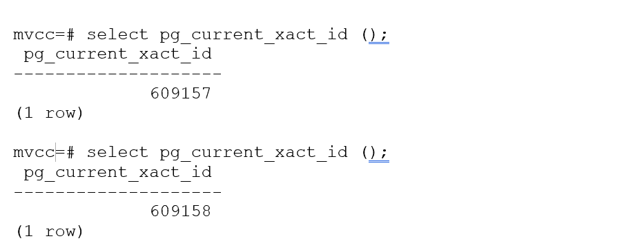
The built-in function pg_current_xact_id() returns the current transaction ID (XID) of the calling session. This call by itself creates a new transaction when you call it for the first time within the unit of work. For example:
A white screen with black text Description automatically generated

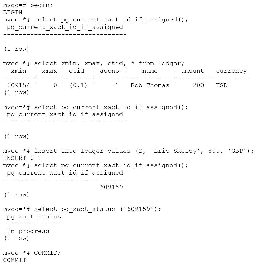
The PostgreSQL transaction manager allocates XID when pg_current_xact_id () is called or an UPDATE, DELETE, INSERT operation is executed. However, a BEGIN transaction or a SELECT operation will not allocate a transaction ID. The built-in function pg_current_xact_id_if_assigned () can be used to return the current transaction ID or NULL if XID is not assigned to the transaction.
A screenshot of a computer code Description automatically generated

A Word About 8-byte Transaction ID (xid8) Enhancement in PostgreSQL

There were enhancements made to the code since PostgreSQL 13 to have a 64-bit (8 bytes) transaction IDs leading up to 9,223,372,036,854,775,808 (9223372 billion transaction IDs compared to 2.2 billion transaction IDs) that does not wrap around during the life of an installation. The following data structures have been modified to make use of 8-byte transaction ID (xid8):

  • PostgreSQL system catalog
  • Functions and procedures
  • Backend worker processes which deal with SQL queries
  • PostgreSQL utilities
  • Replication slots and VACUUM

However, the challenge is to convert an existing XMIN and XMAX data structure from xid4 to xid8 on a running database makes it difficult to perform an in-place conversion. Please look out for more details about xid8 in the future article.

Versioning of Tuples

In PostgreSQL, each tuple (row) in a database table contains two transaction ID (XID) fields known as the xmin and xmax. These fields represent the minimum and maximum transaction IDs that are permitted to see or access a specific row. They play a crucial role in the Multi-Version Concurrency Control (MVCC) mechanism for maintaining data visibility and consistency.

Below are the characteristics of xmin and xmax fields:

xmin (Transaction ID of the creating transaction):

  • The xmin field stores the Transaction ID (XID) of the transaction that created the row version.
  • It indicates the minimum Transaction ID that is allowed to see the row version.
  • Any transaction with a Transaction ID lower than xmin can see and access the row version.
  • xmin is set when a new row version is inserted or created.

xmax (Transaction ID of the deleting transaction):

  • The xmax field stores the Transaction ID (XID) of the transaction that deleted or marked the row version as deleted.
  • It indicates the maximum Transaction ID that is allowed to see the row version.
  • Only transactions with a Transaction ID lower than xmax can see the row version.
  • If xmax is set to infinity (represented as 0), it means the row version is currently not deleted or marked as deleted by any transaction.

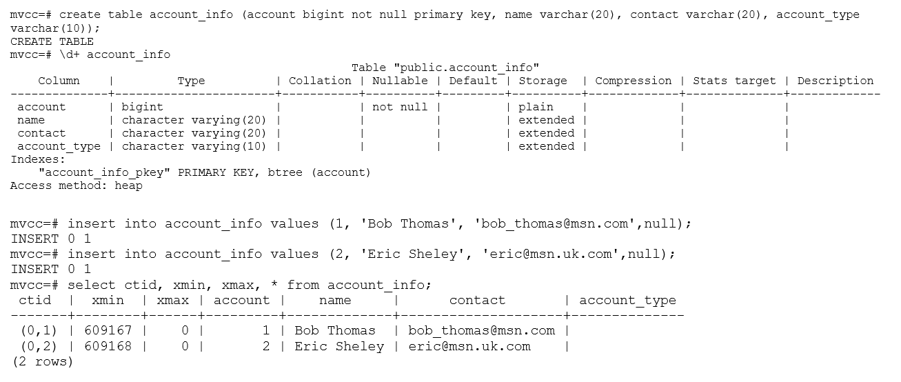
Let’s take an example and see how versioning is maintained in a table.
A close up of a document Description automatically generated

In this example, xmin for the first tuple is 609167. It is the XID of the transaction which inserted this tuple. The xmax column value is set to 0, which means the tuple is active (validity is set to infinity) and there was no update or delete performed on this tuple.

The column ctid is a system column that represents the physical location or address of a row within a table. It consists of two parts: block number and tuple index. The block number identifies the disk block where the row is stored, and tuple index identifies the position of the row within the block.

Figure 1 illustrates a PostgreSQL tuple versioning with a simple example. The session #1 read tuples from table account_info, where xmax was set to infinity (zero) – that means no modifications were made to tuples and were active versions. You will also notice, the ctid is set to (0,1) (0,2) that means both the tuples are stored sequentially in block 0 and this table has only 2 tuples. When session #2 updates the account_type for account=1 tuple, xmin is changed from txid 609167 to 609169 to reflect the transaction performing the update. You will also notice the change in ctid from (0,1) (0,2) to (0,2) (0,3) that means we have 3 tuples in the table stored in block 0. Why do we have 3 tuples in the table when we only see 2 tuples? That’s because PostgreSQL has retained the older version of the tuple for 2 reasons, (1) – there is an open transaction which reads the earlier version of the tuple which is valid between txid 609167 and 609169 and (2) – the recent change is not committed yet from session #2.
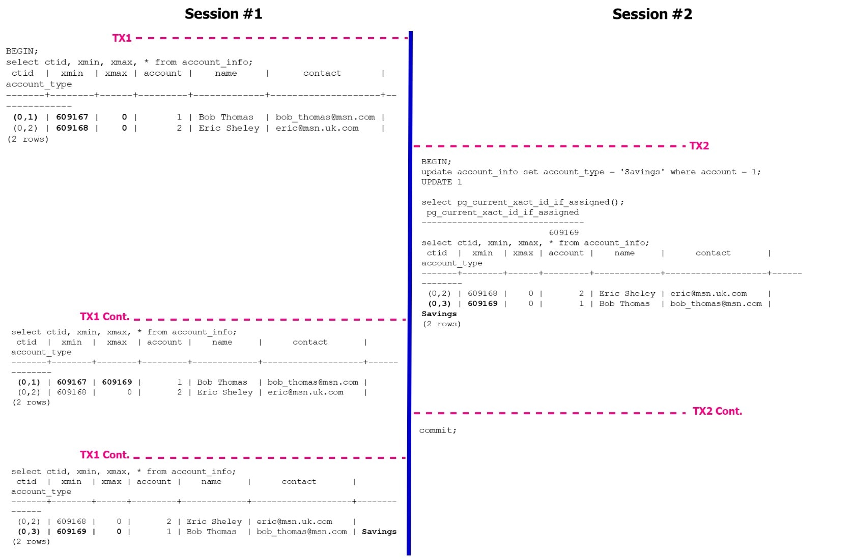
Figure 1: PostgreSQL Versioning Example

The pageinspect module in PostgreSQL provides a set of functions that allow you to inspect and analyze the contents of database pages at a low level. This module is particularly useful for debugging, troubleshooting, and understanding the internal structure of PostgreSQL database pages. For example, we can inspect the table account_info to extract all 3 tuples details (2 active tuples and 1 dead tuple).
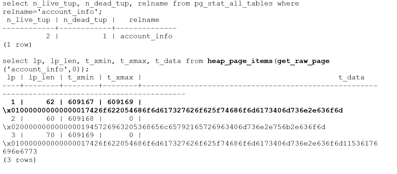
A screenshot of a computer code Description automatically generated

Visibility Check Rules

In PostgreSQL’s Multi-Version Concurrency Control (MVCC) mechanism, visibility check rules are used to determine which data versions are visible to a transaction’s snapshot. These rules ensure that each transaction sees a consistent snapshot of the database as of its start time.

The Visibility Check Rules in PostgreSQL are as follows:

1. Transaction ID (XID) Comparison: Each data version in PostgreSQL has an associated Transaction ID (XID) indicating the transaction that created or modified it. To determine if a data version is visible to a transaction’s snapshot, the following rule is applied:

xmin <= pg_current_xact_id () 
     AND (xmax = 0 OR pg_current_xact_id () < xmax)
  • If the xmin of the data version is lower than the transaction’s XID, it is considered committed before the transaction’s start time and visible to the transaction.
  • If the xmin of the data version is greater than or equal to the transaction’s XID, it is considered not yet committed or modified after the transaction’s start time and not visible to the transaction. However, a tuple will be visible even when xmin > pg_current_xact_id ()with READ COMMITTED isolation level. For example:
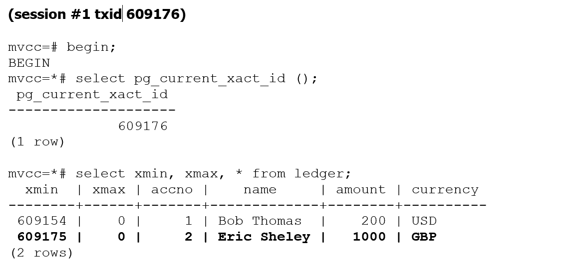
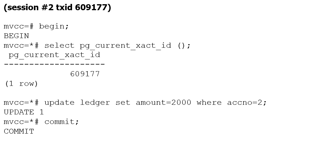
A screenshot of a computer code Description automatically generated

A screenshot of a computer code Description automatically generated

A close-up of a document Description automatically generated

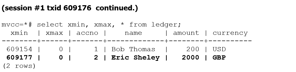
In this example, txid 609176 is still able to view committed data from txid 609177 which is a future transaction id. In PostgreSQL, when a transaction in READ COMMITTED isolation level starts a new query, it takes a new snapshot of the database state. This snapshot represents the committed state of the database at the point in time the query starts. This is the reason for allowing tuples to be visible with xmin > pg_current_xact_id ().

2. Snapshot Transaction ID Range: A transaction’s snapshot includes a transaction ID range that determines the XIDs of the data versions visible to the transaction. For example, you can use pg_current_snapshot () snapshot information function to list the snapshots transaction ID range.

mvcc=# begin;
BEGIN
mvcc=*# update account_info 
set account_type = 'Checking' 
where account = 2;
UPDATE 1
mvcc=*# select pg_current_snapshot();
 pg_current_snapshot
---------------------
 609172:609172:
(1 row)
mvcc=*# select pg_last_committed_xact ();
           pg_last_committed_xact
--------------------------------------------
 (609169,"2023-07-09 01:12:03.883742+00",0)
(1 row)

The snapshot includes the transaction’s own XID and may include a range of other XID values based on the chosen isolation level.

  • Read Committed: A transaction’s snapshot includes its own XID only, allowing it to see only committed data versions that existed before its start time.
  • Repeatable Read: A transaction’s snapshot includes its own XID and all XID values that were already committed at its start time, allowing it to see a consistent snapshot of the data throughout the transaction’s duration.
  • Serializable: A transaction’s snapshot includes a range of XID values up to the transaction’s XID, allowing it to see a consistent snapshot and preventing conflicts with concurrent transactions modifying the same data.

3. Visibility Information: Each data version in PostgreSQL has visibility information associated with it, including the minimum XID (xmin) and the maximum XID (xmax) that are allowed to see the version. These values are used to determine visibility based on the transaction’s snapshot.

  • If the transaction’s XID is greater than xmin, the data version is visible to the transaction.
  • If the transaction’s XID is greater than or equal to xmax, the data version is not visible to the transaction.
  • If xmin is less than the transaction’s XID and xmax is greater than the transaction’s XID, additional checks may be performed to handle special cases, such as in-progress transactions or locks have been held at tuple level.

By applying these visibility check rules, PostgreSQL ensures that each transaction sees a consistent snapshot of the data based on its start time and isolation level. This allows for concurrent access to the database while maintaining read consistency and transaction isolation.

Read Consistency

The read consistency refers to the guarantee that a transaction sees a consistent snapshot of the database as of the transaction’s start time, regardless of concurrent changes made by other transactions. Read consistency ensures that the data accessed by a transaction remains stable and consistent throughout its execution.

Let’s take a closer look at read phenomena, also known as anomalies, are undesirable behaviours that can occur in concurrent database transactions when multiple transactions are reading and modifying the same data concurrently. These phenomena can result in inconsistent or unexpected results if proper isolation and concurrency control measures are not in place.

Dirty Read – This phenomenon can occur during concurrent database transactions. It happens when one transaction reads data that has been modified by another transaction that has not yet been committed. In other words, a transaction reads uncommitted or dirty data. This is completely prevented in PostgreSQL (however this is still possible in other relational database systems such as SQL Server and Db2) and we cannot read uncommitted data.

Non-Repeatable Read – This phenomenon can occur when a transaction reads the same row or tuple multiple times during its execution, but the data values change or vanishes (is deleted) between the reads due to concurrent modifications by other transactions.

Phantom Read – This occurs when a transaction retrieves a set of rows based on a condition, and between consecutive reads, another transaction inserts that satisfy the same condition. As a result, the second read includes additional rows or misses previously retrieved rows, leading to an inconsistent result set.

Serialization Anomaly: This occurs when the outcome of executing a group of transactions concurrently is inconsistent with the outcome of executing the same transactions sequentially in all possible orderings. In other words, the final result of a set of concurrent transactions is not equivalent to any possible serial execution of those transactions.

In PostgreSQL, various transaction isolation levels are available to control the level of concurrency and consistency in database transactions. Each isolation level defines the visibility and locking behavior for concurrent transactions and PostgreSQL supports the following isolation levels:

1. Read Committed (default):

  • Provides read consistency by ensuring that a transaction only sees data that has been committed at the time the query begins.
  • Prevents dirty reads by requiring data to be committed before it becomes visible to other transactions.
  • Allows non-repeatable reads and phantom reads, as concurrent transactions may modify the data between reads.
  • Offers a good balance between consistency and concurrency and is suitable for many applications.

2. Repeatable Read:

  • Provides a higher level of read consistency than Read Committed.
  • Ensures that a transaction sees a consistent snapshot of the database as of the transaction’s start time.
  • Prevents dirty reads and non-repeatable reads by acquiring read locks on accessed data, preventing concurrent modifications.
  • Allows phantom reads, as concurrent transactions may insert new rows that match the query criteria.
  • Provides a stronger guarantee of data consistency but can result in increased concurrency issues due to acquired locks.

3. Serializable:

  • Provides the highest level of isolation and guarantees serializability of transactions.
  • Ensures that concurrent transactions appear as if they were executed serially, without any concurrency anomalies.
  • Prevents dirty reads, non-repeatable reads, and phantom reads.
  • May result in increased locking and potential serialization conflicts, leading to more blocking and reduced concurrency.

Table 1 shows the phenomenon which can occur in a specific isolation level. Even though PostgreSQL allows setting the isolation level to uncommitted, it behaves exactly like read committed.

Isolation Level/Phenomenon

Dirty Read

Non-Repeatable Read

Phantom Read

Serialization Anomaly

READ COMMITTED

Not Possible

Possible

Possible

Possible

REPEATABLE READ

Not Possible

Not Possible

Not Possible

Possible

SERIALIZABLE

Not Possible

Not Possible

Not Possible

Not Possible

Table 1: Transaction Isolation Levels and Read Phenomenon

Let’s look at the Read Committed isolation level and its behavior. Figure 2 illustrates how the dirty read behavior would work. PostgreSQL always reads a committed version of the tuple and dirty reads are not possible. As a side note, you can set the transaction isolation at transactional level or at the database level.

Note: The default isolation level set at the database level is read committed. You can use ALTER DATABASE command to make the change as shown below:

ALTER DATABASE ${dbname} 
   SET DEFAULT_TRANSACTION_ISOLATION TO 'repeatable read';
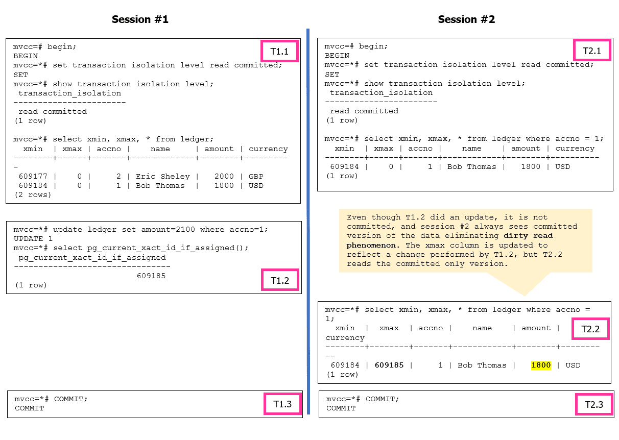
 

Figure 2: Dirty Read phenomenon is not a possibility in PostgreSQL

Figure 3 illustrates the possibility of having non-repeatable read and phantom phenomenon when the isolation level set to READ COMMITTED.
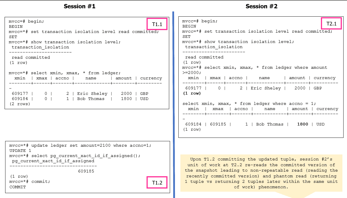
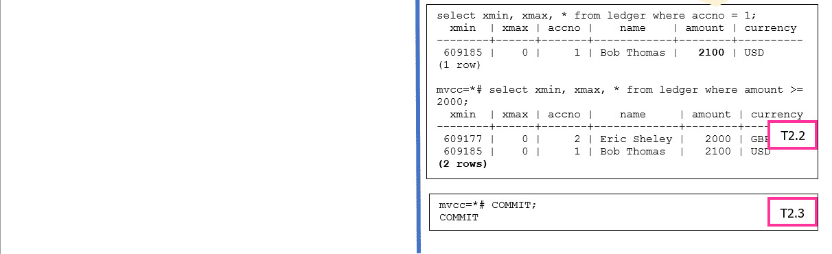
 

Figure 3: Non-Repeatable read and Phantom read phenomenon are possible in PostgreSQL

Let’s look at the Repeatable Read isolation level and its behavior. Figure 4 showcases how PostgreSQL resolves the non-repeatable read and phantom read anomalies. The serialization anomaly can still occur based on how the application is designed.
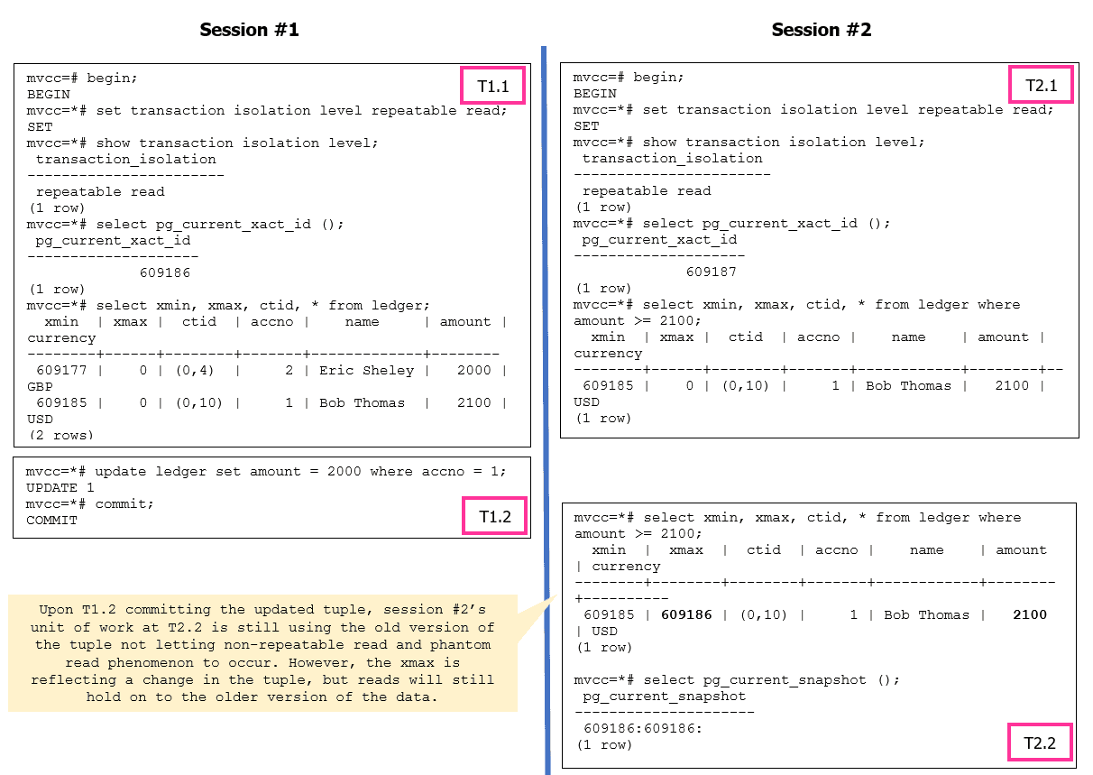

 

Figure 4: Repeatable Read Isolation Level Operations

What happens if an update is attempted to the same tuple from session #2? Let’s try.

mvcc=*# update ledger set amount = 2200 where accno = 1;
ERROR:  could not serialize access due to concurrent update
mvcc=!# select pg_current_snapshot ();
ERROR:  current transaction is aborted, commands ignored until end of transaction block
mvcc=!# rollback;
ROLLBACK

The error message indicates a serialization failure during concurrent transactions. It occurs when two or more transactions attempt to modify the same data simultaneously, resulting in conflicts that violate the strict serializability guarantee.
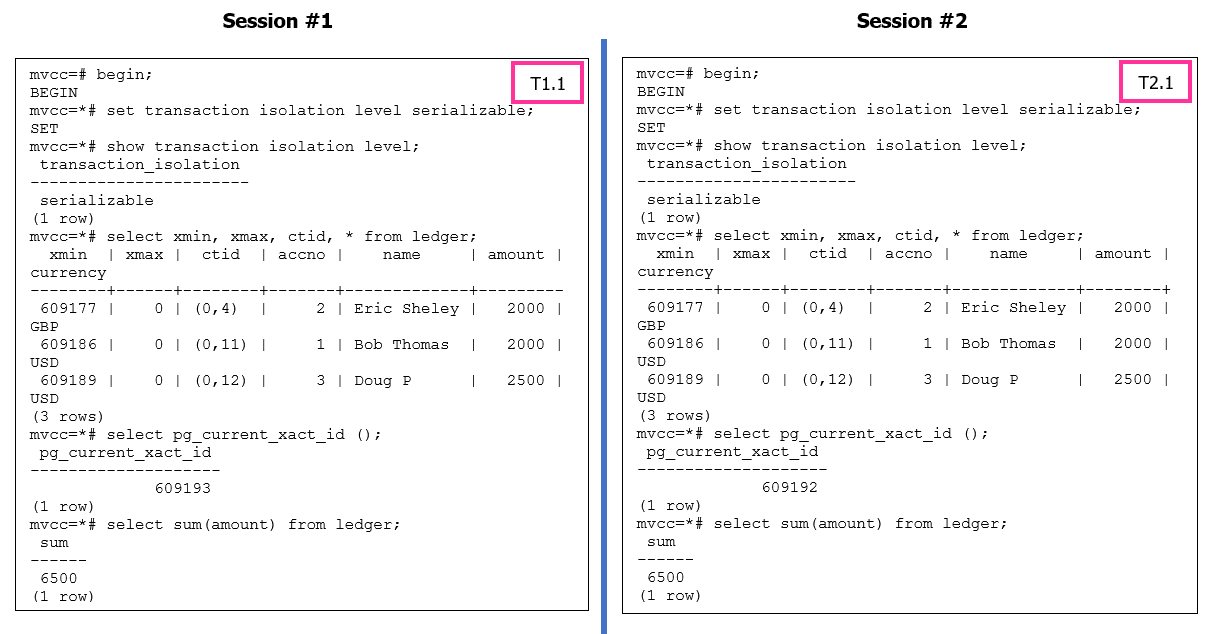
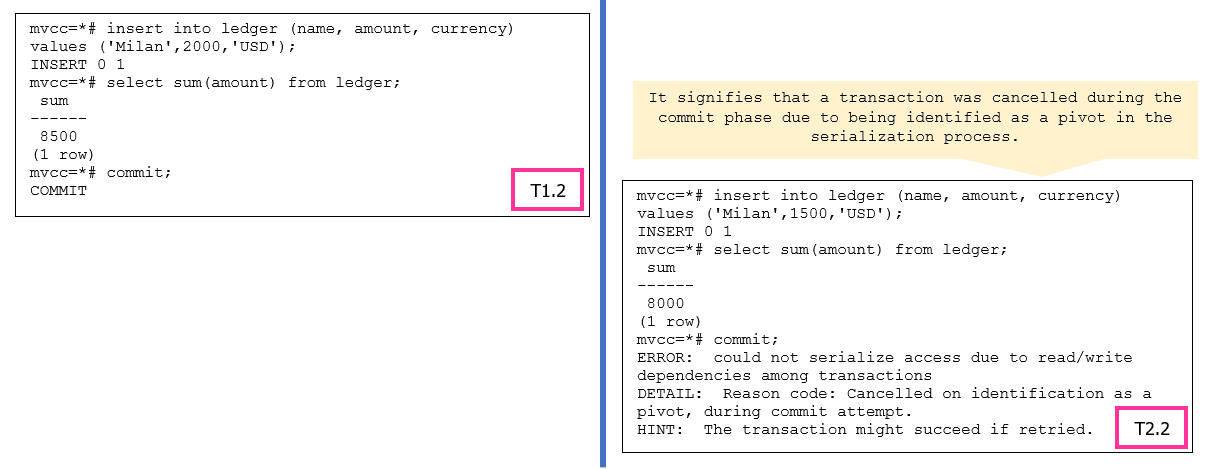
 

Figure 5: Serializable Isolation Level Operations

In PostgreSQL’s SERIALIZABLE isolation level, transactions are executed as if they were running in a serial order, which ensures data consistency. To maintain this strict serializability, PostgreSQL may identify a transaction as a “pivot” when conflicts occur with other concurrent transactions.

A “pivot” transaction is one that serves as a reference point for the serialization process. When conflicts arise, PostgreSQL may choose one transaction as the pivot and abort the other conflicting transactions to preserve consistency. The error message indicates that the transaction being canceled was identified as the pivot during the commit attempt.

For more information, please refer to https://wiki.postgresql.org/wiki/Serializable.

Write Operations

In PostgreSQL databases, an INSERT is simple and no different than other databases. The background writer and WAL writer processes handle the data write operation from shared buffers to the transaction log file and the data pages.

The interest is more in UPDATE and DELETE operations. Let’s take a look at UPDATE operation. When an UPDATE operation in PostgreSQL modifies a row, it follows a multi-version concurrency control (MVCC) mechanism. PostgreSQL will perform a delete and insert internally instead of modifying the existing row in place. This is done to ensure data consistency and handle concurrency control effectively by writers not blocking readers and readers not blocking the writers.

Every UPDATE operation performs pseudo delete, i.e., the original row is marked for deletion, creating a new version of the row with a delete flag. And an insert, a new row is inserted with the updated values, creating a new version of the row.

For simplicity, let’s take an UPDATE example with the READ COMMITTED (default) isolation level. In the example below, either of sessions can start the execution first or can execute both the sessions concurrently.
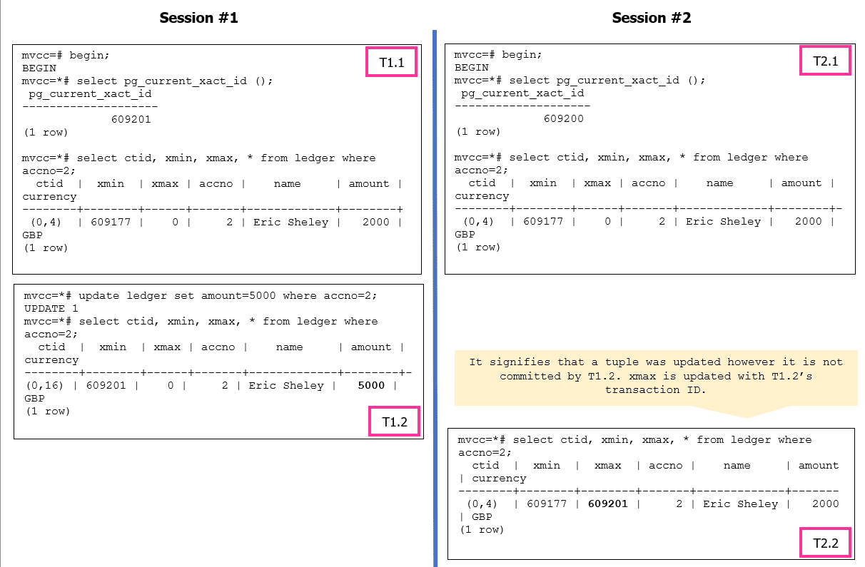
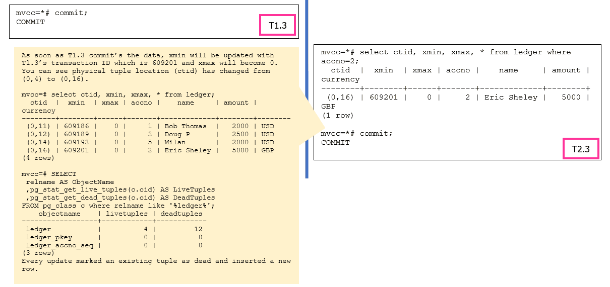
 

The pageinspect module functions can be used to analyze data at page level for both table and indexes. In the case of a DELETE operation, the xmax will be updated with the transaction id which executes the DELETE and marks the tuple as dead.

Garbage Collection

In PostgreSQL, garbage collection refers to the process of reclaiming disk space occupied by deleted or obsolete data. When data is deleted or updated in PostgreSQL, it is not immediately removed from the disk. Instead, it is marked as eligible for garbage collection, and the actual disk space is reclaimed later by the autovacuum process.

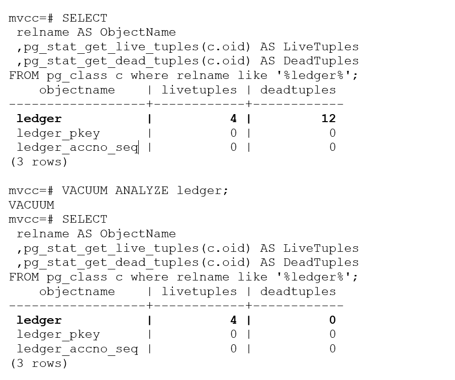
Based on our example, we have 4 live tuples and 12 dead tuples, these dead tuples can be cleaned using VACUUM. The VACUUM command is used to perform a table vacuum (data reorganization). It reclaims disk space by physically reorganizing the table and its associated indexes, and it can be more resource-intensive compared to regular VACUUM operations.

mvcc=# VACUUM VERBOSE ledger;
INFO:  vacuuming "mvcc.public.ledger"
INFO:  finished vacuuming "mvcc.public.ledger": index scans: 1
pages: 0 removed, 1 remain, 1 scanned (100.00% of total)
tuples: 12 removed, 4 remain, 0 are dead but not yet removable
removable cutoff: 609251, which was 0 XIDs old when operation ended
index scan needed: 1 pages from table (100.00% of total) had 12 dead item identifiers removed
index "ledger_pkey": pages: 2 in total, 0 newly deleted, 0 currently deleted, 0 reusable
avg read rate: 0.000 MB/s, avg write rate: 0.000 MB/s
buffer usage: 11 hits, 0 misses, 0 dirtied
WAL usage: 4 records, 1 full page images, 8480 bytes
system usage: CPU: user: 0.00 s, system: 0.00 s, elapsed: 0.00 s
VACUUM

However, the dead tuple count is still showing as 12 in the catalog. This is just the system catalog information and we will have to execute the ANALYZE command to update table statistics, including information about the distribution of data, column histograms, and correlation between columns. These statistics are used by the query optimizer to generate efficient execution plans
Summary:

MVCC (Multi-Version Concurrency Control) is a concurrency control mechanism used in PostgreSQL to handle concurrent access to data. It allows multiple transactions to read and write data concurrently while maintaining transaction isolation and ensuring consistency. In this article we learnt MVCC specifics and the building blocks of MVCC in detail. We will dive deep into each section such as VACUUM internals, storage internals, index B tree internal and locking internals in the future articles.


The post Database Concurrency in PostgreSQL appeared first on Simple Talk.


from Simple Talk https://ift.tt/4jq15EB
via
Friday, August 11, 2023

Going to a conference where hardly anybody knows my name

On Friday and Saturday August 11 and 12, I am going to do something I haven’t done in a long time. I am going to a conference where I may not know anyone (I did learn about the conference from one of the people that run it who was also at SQL Saturday Baton Rouge.) I am going to Powershell On The River in Chattanooga, TN and I am pretty excited to go and learn some more about PowerShell.

They have a first day of 1/2 day sessions, starting with the one I am excited about “Develop Your First Module.” I am not a newbie at PowerShell (though I haven’t used it seriously in a few years), but I am not even going to pretend I am 100% sure what defines a module! The day will hopefully progress to a session called “1up PowerShell for Extra Life” which looks like a nice coverage of all the basic topics I need. 

The only time I will not be happy about this is that the first session starts at 9:00 AM, and I will need to leave at 7;30 or so to be guaranteed to get there on time. I am not a morning person.

Saturday is a more typical conference set up with hour long sessions that are largely about PowerShell and a few other computing topics.

Of course, my reason for going to this conference is only partially so I can write better PowerShell. I want to meet some of this community and maybe hand out a business card or two.

If you know me (and especially if you have ever been exhorted by me to write), you will know two things are true. First, I am really introverted. Two, while I am less introverted once I have met people, I am not pushy. 

So going to a conference where I don’t know anyone is going to be an adventure. The last time I remember doing this was in the early 2000’s when I first started going to PASS. It took me a while to make the contacts and friends I have today. So who knows what will come of this weekend. In any case I hope to find new people’s blogs to read and some Powershell skills.

If you want to write about Powershell (or data, or programming…), check out the details on the About Simple Talk page. 

The post Going to a conference where hardly anybody knows my name appeared first on Simple Talk.


from Simple Talk https://ift.tt/7jTupoB
via
Wednesday, August 9, 2023

A Beginners Guide to MySQL Replication Part 4: Using GTID-based Replication

Welcome back to another replication series! As a quick reminder, we explored various methods of using MySQL’s replication capabilities in our previous discussions. Initially, we employed the traditional binary-log-based replication approach to set up our replication servers. This involved tracking the binary log file and its positions to facilitate replication.

In this article, we will dive into a more recent and acceptable approach to creating replication – using the Global Transaction Identifiers (GTID) based replication.

WHY Global Transaction Identifiers (GTIDs)?

GTIDs (Global Transaction Identifiers) provide a way to uniquely identify and track transactions across a distributed database environment. Each server assigns a unique GTID to every transaction, which greatly makes managing and coordinating data replication between multiple MySQL servers super easy. Here are some reasons why we use GTIDs in MySQL:

1. Unique Identification

GTIDs offer a distinct and globally unique identification for each transaction within a distributed database environment, as long as the transaction was recorded in the binary log. If a transaction is not written to the binary log, such as a read-only transaction, the system won’t assign it a GTID. This uniqueness guarantees that every transaction has a one-of-a-kind identifier, simplifying the process of monitoring and handling data modifications.

2. Data Consistency

GTIDs play a vital role in upholding data consistency across distributed databases. It ensures that a transaction committed on the source server cannot be duplicated on the replica, guaranteeing that transactions are applied in the precise order they were executed. As a result, data synchronization remains accurate and consistent across all servers involved.

3. Replication-made-easy

 GTIDs make the replication process between MySQL servers much simpler. With GTID-based replication, you don’t need to manage complex binary log positions; servers can easily identify which transactions have been applied and which are pending replication.

4. Failure and Recovery

 In case of server failures or crashes, GTIDs help ensure that data is consistently replicated. After a failure is resolved, the replication process can automatically resume from the last successfully applied GTID. This helps prevent data inconsistencies.

5. Easy to track

GTID-based replication simplifies tracking the source server of any transaction. By assigning a unique GTID to each transaction, which includes the source server’s unique identifier (server UUID) and the transaction sequence number, we can easily extract and decode the GTID from the binary log of a GTID-based transaction, thereby determining the original server. This capability is invaluable for auditing, troubleshooting, and maintaining data integrity in distributed database environments.

Configuring Replication with GTIDs

Configuring replication with GTIDs in MySQL involves several steps. Below is a step-by-step guide to help you set up GTID-based replication:

1. Configure the source server

To configure each MySQL server that would be participating in the replication setup, you must assign a unique server ID, set up a binary log, enable GTID mode, and create a replication user on the source server. Here’s what you need to do:

i. Assign a unique server ID: If the server ID is not assigned or you want to change it, you can do so by adding the following line in my.cnf or my.ini file under the [mysqld] section:

server_id = YOUR_UNIQUE_SERVER_UUID

Replace YOUR_UNIQUE_SERVER_UUID with a universally unique identifier (UUID).

ii. Enable GTID Mode: To start using GTIDs, you must enable GTID mode in the MySQL configuration file (my.cnf or my.ini). Add the following line under the [mysqld] section:

gtid_mode = ON
enforce-gtid-consistency=ON
--skip-slave-start=ON

The option --skip-slave-start=ON is employed to delay the start of replication until the replica is fully configured. Save the configuration file and restart the MySQL server.

iii. Binary Logging: Ensure that binary logging is enabled on the source server. This is necessary for GTID-based replication to function properly.

log_bin = /path/to/binary/log/file

iv. Create Replication User: As part of the configuration, you need to create a dedicated user on the source server that the replica servers will use to connect and replicate data. Grant the necessary privileges to this user using the following SQL command:

CREATE USER 'replication_user'@'replica_host' 
IDENTIFIED BY 'your_password'; 

GRANT REPLICATION SLAVE ON *.* TO 'replication_user'@'replica_host'; 

FLUSH PRIVILEGES;

Replace 'replication_user', 'replica_host', and 'your_password' with appropriate values. The FLUSH PRIVILEGES command is used to ensure that the server reloads the grant tables after granting the necessary privileges to the new user. This is necessary because the changes to the user privileges are stored in the MySQL grant tables, and these tables are cached in memory for performance reasons.

2. Configure the replica server

To configure the replica server using a GTID-based transaction, a unique server ID is required, else, the replication wouldn’t function properly. Here’s what we need to do:

i. Set Server UUID: If the server UUID of the replica server is different from the source server, you need to set it. Add the following line to my.cnf or my.ini file under the [mysqld] section:

server_uuid = YOUR_UNIQUE_SERVER_UUID

Replace YOUR_UNIQUE_SERVER_UUID with a universally unique identifier (UUID).

ii. Enable GTID Mode: Open the MySQL configuration file (my.cnf or my.ini) on the replica server, and under the [mysqld] section, add the following line to enable GTID mode:

gtid_mode = ON
enforce-gtid-consistency=ON
log-replica-updates=ON

iii. Binary Log: Replica servers are allowed to use GTID without configuring binary logs. If you wish to continue without enabling this, you can use the --skip-log-bin and --log-replica-updates=OFF options. However, to ensure that the binary log is enabled on the replica server. Add the following line to my.cnf or my.ini file:

log_bin = /path/to/binary/log/file

Replace /path/to/binary/log/file with the desired location for storing binary logs.

iv. Restart MySQL Server: Save the changes made to the configuration file and restart the MySQL server on the replica to apply the changes.

3. Start replication on the replica server

Once the source and replica servers are configured, we can start the replication process on the replica server. Connect to the replica server’s MySQL console and issue the following command:

--For MySQL versions lesser than 8.0.23

CHANGE MASTER TO MASTER_HOST = 'source_server_ip',
MASTER_PORT = source_server_port, MASTER_USER = 'replication_user', 
MASTER_PASSWORD = 'your_password', MASTER_AUTO_POSITION = 1, 
master_info_repository=TABLE, relay_log_info_repository=TABLE ;


--For MySQL version 8.0.23 or greater 

CHANGE REPLICATION SOURCE TO SOURCE_HOST = 'source_server_ip', 
SOURCE_PORT = source_server_port, SOURCE_USER = 'replication_user',
SOURCE_PASSWORD = 'your_password', SOURCE_AUTO_POSITION = 1;

Replace 'source_server_ip', source_server_port, 'replication_user', and 'your_password' with the appropriate values.

The replica has a special place where it keeps important information needed to read and apply changes from the original server. This information is used by a specific part of the replica called the “applier metadata repository” to understand what changes it has already processed and what still needs to be done. This information includes things like file names and positions, which help the applier metadata repository keep track of where it is in the process of replicating data and is stored within the slave_relay_log_info table in the MySQL system schema. It’s like a road map to follow.

Before MySQL 8.0, if you wanted to use tables as replication metadata repositories, you had to explicitly set the master_info_repository and relay_log_info_repository options to TABLE during server startup.

Starting from MySQL 8.0, creating the replication metadata repositories as tables became the default behavior. As a result, you no longer need to set these system variables to use tables for the replication metadata repositories. However, it’s important to note that the use of master_info_repository and relay_log_info_repository system variables is deprecated in MySQL 8.0 and may be removed in future versions. So, it’s recommended to rely on the default table-based replication metadata repositories instead.

4. Backup Data

Before starting replication, it’s essential to ensure that the replica server has the same data as the source server. You can use tools like mysqldump or Percona XtraBackup to create a backup on the source server and restore it on the replica server.

5. Start replica server

After setting up replication parameters, you can start the replica server by executing the following command:

-- For MySQL versions lesser than 8.0.23
START SLAVE;

--For MySQL version 8.0.23 or greater
START REPLICA;

You can monitor the  replica server’s status using the following command:

-- For MySQL versions lesser than 8.0.23
SHOW SLAVE STATUS \G

--For MySQL version 8.0.23 or greater 
SHOW REPLICA STATUS;

Look for the Slave_IO_Running and Slave_SQL_Running status variables to ensure that both are set to Yes, indicating that the replication is running correctly.

Once you have completed these steps, your MySQL replication with GTIDs should be up and running! 

Configuring Multi-Source Replication using GTIDs

To configure a replication channel for each source using a GTID-based replication, on each MySQL server, we need to identify the source servers from which they will replicate data. This is typically done by specifying the source server’s connection details, including the server’s unique ID and the login credentials in the configuration file. Then, we can enable multi-source replication by specifying the following commands:

--For MySQL version 8.0.23 or less, the following command is applicable
--Replication path for source server 1 
CHANGE MASTER TO MASTER_HOST=”source_server1”,
MASTER_USER=”user_name”, MASTER_PASSWORD=”password”,
MASTER_AUTO_POSITION=1 FOR CHANNEL “source_server1”;

--Replication path for source server 2
CHANGE MASTER TO MASTER_HOST=”source_server2”,
MASTER_USER=”user_name”, MASTER_PASSWORD=”password”,
MASTER_AUTO_POSITION=1 FOR CHANNEL “source_server2”;

--Replication path for source server 3
CHANGE MASTER TO MASTER_HOST=”source_server3”,
MASTER_USER=”user_name”, MASTER_PASSWORD=”password”,
MASTER_AUTO_POSITION=1 FOR CHANNEL “source_server3”;


--For MySQL version 8.0.23 or greater, the following command is applicable 
--Replication path for source server 1 
CHANGE REPLICATION SOURCE TO SOURCE_HOST=”source_server1”, 
SOURCE_USER=”user_name”, SOURCE_PASSWORD=”password”,
SOURCE_AUTO_POSITION=1 FOR CHANNEL “source_server1”; 

--Replication path for source server 2 
CHANGE REPLICATION SOURCE TO SOURCE_HOST=”source_server2”,
SOURCE_USER=”user_name”, SOURCE_PASSWORD=”password”, 
SOURCE_AUTO_POSITION=1 FOR CHANNEL “source_server2”; 

--Replication path for source server 3 
CHANGE REPLICATION SOURCE TO SOURCE_HOST=”source_server3”,
SOURCE_USER=”user_name”, SOURCE_PASSWORD=”password”, 
SOURCE_AUTO_POSITION=1 FOR CHANNEL “source_server3”;

To replicate the database of our choice, this can be achieved using the CHANGE REPLICATION FILTER statement. 

--To replicate the database of our choice

CHANGE REPLICATION FILTER REPLICATE_WILD_DO_TABLE=(‘database1.%’)
FOR CHANNEL “source_server1”;

CHANGE REPLICATION FILTER REPLICATE_WILD_DO_TABLE=(‘database2.%’)
FOR CHANNEL “source_server2”;

CHANGE REPLICATION FILTER REPLICATE_WILD_DO_TABLE=(‘database3.%’) 
FOR CHANNEL “source_server3”;

And this is how you configure multi-source replication in a GTID-based replication.


Drawbacks of GTID-based replication

Replication with GTID (Global Transaction Identifier) in MySQL offers several advantages, such as simplifying the configuration and improving reliability. However, there are certain restrictions and considerations to be aware of:

  1. GTID Mode: Replication using GTID requires all servers in the replication topology to be running in GTID mode. Mixing GTID and non-GTID servers is not supported.
  2. Server Version: GTID was introduced in MySQL 5.6.5. To use GTID-based replication, all servers involved must be running MySQL 5.6.5 or later versions.

  3. GTID Consistency: For proper replication, the GTID consistency across all servers must be maintained. If GTIDs are manipulated manually, it can lead to data inconsistency and replication errors.
  4. Temporary Tables: GTID-based replication does not support temporary tables on the slave. If you have temporary tables in your replication, you might need to restructure your schema.
  5. Unsupported CREATE TABLE AND SELECT STATEMENTS: The CREATE TABLE AND SELECT statements are not supported when using the GTID-based replication topology due to inconsistencies with the statement and row replication formats.


Conclusion

With GTID, replication setup becomes more straightforward, as there is no need to deal with file and position values. It also enhances data integrity and reliability by supporting ROW-based replication, eliminating the issues associated with non-deterministic statements. However, implementing GTID-based replication requires careful planning and consideration of certain restrictions as mentioned earlier. It is essential to be aware of the limitations, especially concerning temporary tables,  to avoid unexpected challenges during deployment or changes in the replication topology.

When used correctly and in suitable scenarios, GTID-based replication proves to be a valuable tool for managing replication environments, offering greater confidence in data synchronization and replication reliability. For additional information on GTID-based replication, I highly suggest you visit the MySQL official documentation.


The post A Beginners Guide to MySQL Replication Part 4: Using GTID-based Replication appeared first on Simple Talk.


from Simple Talk https://ift.tt/I3BVgEm
via
Tuesday, August 8, 2023

T-SQL Tuesday #165 – My Experience with Database Job Titles

They mean very little.

More on that after nothing that this is part of T-SQL Tuesday, and you can read the original invitation by clicking on the T-SQL Tuesday 165 invitation or the following images. I almost always forget that this is coming and today is no different. But I wanted to chime in here.

T-SQL Tuesday 165 - Database job titles are in the eye of the beholder

By “very little”, I don’t mean that if you take a job as a DBA, you will likely be repurposed to wash dishes for the CEO’s birthday party. What I mean is that many of the definitions of a DBA and other database professionals have a lot of overlap in their definitions.

For example, as I looked around for formal definitions, I found a few interesting ones:

Oracle.com stated:

A database administrator, or DBA, is responsible for maintaining, securing, and operating databases and also ensures that data is correctly stored and retrieved.

This is the start of a good definition. But that definition is very, very wide. In fact, later in the same page, it lists different types of DBAs, which include system, database architects, analysts, modelers, application, task-oriented…

Craig S Mullins on TechTarget said:

A database administrator (DBA) is the information technician responsible for directing and performing all activities related to maintaining a successful database environment. A DBA makes sure an organization’s databases and related applications operate functionally and efficiently.

I like this description, and reading the entire article, you can see a very optimistic definition of what DBAs do.

When adopting a new DBMS, the DBA is responsible for designing, implementing and maintaining the database system. Often, that includes installing the DBMS and setting up the IT infrastructure to allow applications to access databases.

Of course, if this were true, so many DBA types wouldn’t spend so much energy complaining about how developers make their own databases and, too often, how our database servers are running on hardware more realistically fit for a file server. If more of us had proper database server hardware, the move to the cloud database would have happened less quickly. Still, we surrendered to get the hardware we begged for.

So, what of a title like Database Reliability Engineer? Gitlab had this to say about their use of the term:

Database Reliability Engineers (DBRE) are responsible for keeping database systems that support all user-facing services (most notably GitLab.com) and many other GitLab production systems running smoothly 24/7/365.

Digging into the definition, though, it sounds more like what a DBA really did in my world. Maintained the server, made sure it didn’t crash (and if it did that you could get it back up and running as fast as possible), and provided support for teams to make sure they wrote decent code:

Provide database expertise to engineering teams (for example through reviews of database migrations, queries and performance optimizations).

Of course, telling the engineering teams that their queries are not great is always a fun use of an afternoon.

Before coming to Redgate, my title was Data Architect for the past 15 or so years.

Coursera.org says a data architect is:

IT professionals who leverage their computer science and design skills to review and analyze the data infrastructure of an organization, plan future databases, and implement solutions to store and manage data for organizations and their users.

I mean, I did some of that, especially designing most of the new databases for the organization. But if I am honest, most of my career was spent doing that last thing. “Implement solutions.” This, I am pretty sure, translates to “writing database and ETL code.” In their first bullet point for defining the tasks, it states: “Translating business requirements into databases, data warehouses, and data streams.“

In my experience (which was not on a vast number of teams, admittedly), once you start doing something practical on any regular basis, it is hard to do a lot of the higher-level planning kinds of tasks that don’t move current processes forward. Think of any task you do now that wasn’t part of your original job title, and how you acquired it. Same thing.

So many titles, so very similar

In the T-SQL Tuesday host blog, there is a list of titles, DBA, Database Engineer, Database Reliability Engineer, Data Architect, Database Architect, Data Warehouse Architect, Data Warehouse Engineer, that all could mean kind of the same thing, depending on just how large of an organization you work with and what they think it means. If you work for a company that actually has one of each, the distinctions would likely be noticeable. You will also be in a very huge organization!

But even in SQL Kitty’s entry (AKA Josephine Bush, newly minted Microsoft MVP!) if you read the list presented there is so much overlap in her definitions, just like the one’s I have quoted.

Quick Aside: On my drive to and from SQL Saturday Baton Rouge the other day, I listened to the Primary Phase of the Hitchhiker’s Guide to the Galaxy Radio Series. Why I mention this will become apparent if you have listened to or read the book. If not, I will simply warn you in advance that dingo’s kidneys are not at all a pleasant thing.

While my personal experience on teams was not widespread, I have met and talked to a lot of people about what they do over the years, and most titles that people have are a load of dingo’s kidneys. In general, most titles are largely concerned with the movement of small green pieces of paper, which is odd because the pieces of paper don’t have as much to do with the database operations as things like normalization and testing. Titles are very often picked to position an employee with an associated salary.

One Distinctive Data Title

Really the one data-oriented title that has come out in recent years that really stands out as something different has been Data Scientist. To me, this is a pure coding and math-based profession, doing the kind of analysis that most data professionals only dream about as they are mucking around in the data trying to find out why Zaphod’s Gargleblaster was 2.35 Alturian dollars instead of 2.33 (ah, rounding issues). When the database systems crashes, all of the other folks with data in their title will be involved because they work below the surface of the database and infrastructure.

Techopedia defined a data scientist as:

A data scientist is an individual, organization, or application that performs statistical analysis, data mining, and retrieval processes on a large amount of data to identify trends, figures and other relevant information.

Skipping past that “or application” part that sounds ominously like SkyNet, the focus is on working with the data and using math to find real information from it. When I first heard about the concept of a data scientist, I was really interested. Then I realized you probably needed to really understand statistical analysis… and I don’t.

Conclusion

If you are applying for a job with any of these titles… look at what they want you to actually do. Twice. Then ask. There is a chance that what Company X means by Database Administrator and what someone else at Company X means by the same term. Branch out into other positions, and the Database Reliability Engineer could be simply that, making sure the database systems are reliable.

Just remember, if your full-time job is handling the reliability of any system, one of two things is true. The system is a mess. You won’t end up actually doing that full-time if you are good at it.


The post T-SQL Tuesday #165 – My Experience with Database Job Titles appeared first on Simple Talk.


from Simple Talk https://ift.tt/2XdZPGy
via
Monday, August 7, 2023

What Is an Execution Plan and How to Find It in PostgreSQL

In the last blog (When PostgreSQL Parameter Tuning is not the Answer), we compared several execution plans for a SQL statement as we made changes to parameters and indexes. Still, there was no mention of what an execution plan is, how one can obtain an execution plan for a query, and how to interpret the result. In this blog, we will take a deep dive into this topic.

Why we need an execution plan?

Most likely, if you ever worked with any relational DBMS, you heard the term execution plan, and moreover, you might have seen some of them. But have you ever thought about why you might need an execution plan for a SQL statement? Why you never need to (or get to) produce an execution plan for your C or Java program? The reason is that SQL is a declarative language. That means that when we write a SQL statement, we describe the result we want to get, but we don’t specify how that result should be obtained.

By contrast, in an imperative language (like C), we specify what to do to obtain a desired result—that is, the sequence of steps that should be executed. Sometimes it may not look like it when using modern languages, but once compiled they generally do the steps you program them to.

Note: If you want to execute the samples, in the last section of the article is an appendix with the instructions for preparing the demo.

What is an execution plan?

So, we just sent a SQL statement for PostgreSQL to execute it. Let’s use the same statement we used to illustrate the previous blog:

SELECT f.flight_no,
       f.actual_departure,
       count(passenger_id) passengers
  FROM postgres_air.flight f
       JOIN postgres_air.booking_leg bl 
          ON bl.flight_id = f.flight_id
       JOIN postgres_air.passenger p 
        ON p.booking_id=bl.booking_id
 WHERE f.departure_airport = 'JFK'
   AND f.arrival_airport = 'ORD'
   AND f.actual_departure BETWEEN
        '2023-08-08' and '2023-08-12'
GROUP BY f.flight_id, f.actual_departure;

We sent this to PostgreSQL to execute – what happens next?

To produce query results, PostgreSQL performs the following steps:

  • Compile and transform a SQL statement into an expression consisting of high-level logical operations, known as a logical plan.
  • Optimize the logical plan and convert it into an execution plan.
  • Execute (interpret) the plan and return results.

Compiling a SQL query is similar to compiling code written in an imperative language. The source code is parsed, and an internal representation is generated. However, the compilation of SQL statements has two essential differences.

First, in an imperative language, the definitions of identifiers are usually included in the source code, while definitions of objects referenced in SQL queries are mostly stored in the database. Consequently, the meaning of a query depends on the database structure: different database servers can interpret the same query differently.

Second, the output of an imperative language compiler is usually (almost) executable code, such as byte code for a Java virtual machine. In contrast, the output of a query compiler is an expression consisting of high-level operations that remain declarative—they do not give any instruction on how to obtain the required output. A possible order of operations is specified at this point, but not the manner of executing those operations. The logical plan for the SQL statement presented above is shown below:

project f.flight_no,  f.actual_departure, count(p.passenger_id)[] (
   group [f.flight_no, f.actual_departure] (
      filter [f.departure_airport = 'JFK'] (
         filter [f.arrival_airport = 'ORD'] (
            filter [f.actual_departure >='2023-08-08'](
               filter [f.actual_departure <='2023-08-12' ] (
                  join [bl.flight_id = f.flight_id] (
                     access (flights f),
                     join(bl.booking_id=p.booking_id (
                     access (booking_leg bl),
                     access (passenger p)
                     ))))))))

Here, project stands for relational operation projection, which reduces the number of columns in the output; filter stands for relational operation filter, which applies selection criteria, join stands for join operation, access identifies that we need to read data from database tables. Note, that the representation above is a “humanized” version of PostgreSQL internal representation of the logical plan, and there is no command that would allow you to actually “see” it.

The instructions on how to execute the query appear at the next phase of query processing, optimization. An optimizer performs two kinds of transformations: it replaces logical operations with their execution algorithms and possibly changes the logical expression structure by changing the order in which logical operations will be executed.

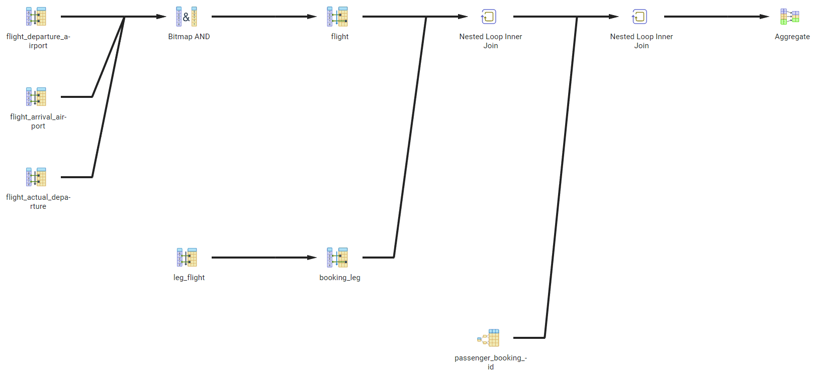
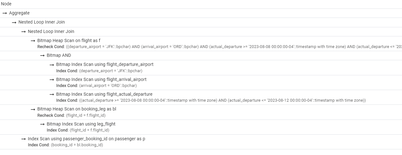
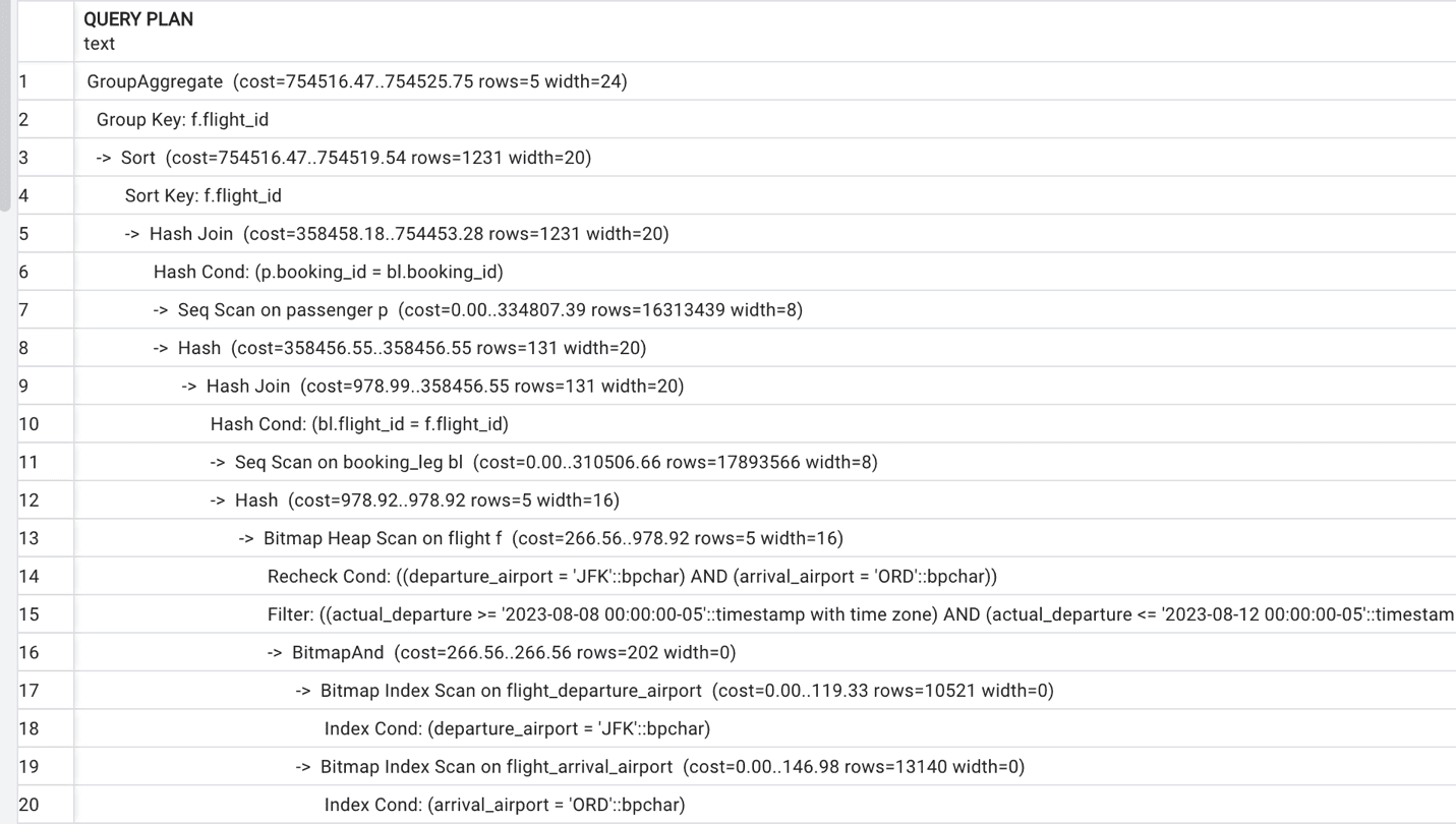
Then, it tries to find a logical plan and physical operations that minimize required resources, including execution time. In this blog, we won’t go into details of how these transformations are done and how the optimizer decides which plan is the best, but we will look at some examples in subsequent blogs. The only thing we need to know now is that the output of the optimizer is an expression containing physical operations. This expression is called a (physical) execution plan. For that reason, the PostgreSQL optimizer is often called the query planner. There are multiple ways you can obtain the physical execution plan for a query, and they will be described later in this blog.

Finally, the query execution plan is interpreted by the query execution engine, frequently referred to as the executor in the PostgreSQL community, and output is returned to the client application.

How is an execution plan built?

The job of the optimizer is to build the best possible physical plan that implements a given logical plan on the server it is executing on. This is a complex process: sometimes, a complex logical operation is replaced with multiple physical operations, or several logical operations are merged into a single physical operation.

To build a plan, the optimizer uses transformation rules, heuristics, and cost-based optimization algorithms. A rule converts a plan into another plan with better cost. For example, filter and project operations reduce the size of the dataset and therefore should be executed as early as possible; a rule might reorder operations so that filter and project operations are executed sooner.

An optimization algorithm chooses the plan with the lowest cost estimate. However, the number of possible plans (called the plan space) for a query containing several operations is huge—far too large for the algorithm to consider every single possible plan, so heuristics are used to reduce the number of plans evaluated by the optimizer.

How to obtain the execution plan?

There are multiple ways to find out the execution plan of any SQL statement, not only SELECT, but also INSERT, UPDATE and DELETE.

The easiest way is to run EXPLAIN command and pass the SQL statement to it:

EXPLAIN SELECT f.flight_no,
       f.actual_departure,
       count(passenger_id) passengers
  FROM postgres_air.flight f
       JOIN postgres_air.booking_leg bl 
          ON bl.flight_id = f.flight_id
       JOIN postgres_air.passenger p 
        ON p.booking_id=bl.booking_id
 WHERE f.departure_airport = 'JFK'
   AND f.arrival_airport = 'ORD'
   AND f.actual_departure BETWEEN
        '2023-08-08' and '2023-08-12'
GROUP BY f.flight_id, f.actual_departure;

The result will be a projected execution plan. Remember that in contrast to Oracle or MS SQL Server, PostgreSQL query planner always produces the execution plan right before the execution itself based on many factors, including the current database statistics. (Other RDBMS platforms may reuse previously calculated plans which can have negative, and positive, effects.)

When you execute EXPLAIN PostgreSQL projects the costs of the operations based on the available statistics, which might be not current (or at least, may be in a different state when you actually execute your query to get back data.) Still, running EXPLAIN command would give you a good idea of how your query will be executed.

Another version of the EXPLAIN command is EXPLAIN ANALYZE:

EXPLAIN ANALYZE SELECT f.flight_no,
       f.actual_departure,
       count(passenger_id) passengers
  FROM postgres_air.flight f
       JOIN postgres_air.booking_leg bl 
          ON bl.flight_id = f.flight_id
       JOIN postgres_air.passenger p 
        ON p.booking_id=bl.booking_id
 WHERE f.departure_airport = 'JFK'
   AND f.arrival_airport = 'ORD'
   AND f.actual_departure BETWEEN
        '2023-08-08' and '2023-08-12'
GROUP BY f.flight_id, f.actual_departure;

This command produces an execution plan and executes the statement (but does not output the execution results). This allows us to see not only the estimated statistics, but how long the execution took in reality and which original estimates were not right.

Finally, we can run EXPLAIN command with multiple parameters, which are listed below:

  • ANALYZE [ Boolean ] – includes actual execution.
  • VERBOSE [ Boolean ] – provides more details about plan steps.
  • COSTS [ Boolean ] The COSTS parameter defaults to TRUE, including actual when ANALYZE is included– displays projected and actual cost of each plan node (operation in the query).
  • SETTINGS [ Boolean ] – list of modified configuration parameters.
  • BUFFERS [ Boolean ] – Only used when ANALYZE is included, shows the usage of the shared buffers.
  • WAL [ Boolean ] – Only used when ANALYZE is included, shows the effect of WAL (Write ahead logging).
  • TIMING [ Boolean ] – Only used when ANALYZE is included, – shows execution time for each node of the query plan.
  • SUMMARY [ Boolean ] – default TRUE when ANALYZE]- prints the summary
  • FORMAT { TEXT | XML | JSON | YAML } – execution plan output format

As an example, you could use the following:

EXPLAIN ( ANALYZE, VERBOSE, FORMAT XML )
SELECT…

And get the physical execution plan, with verbose details, in an XML format. You can find more information on the SQL Explain page of the PostgreSQL documentation. But EXPLAIN and EXPLAIN ANALYZE will be the two command you will typically use the most.

How to read an execution plan?

Now, let’s finally get back to the execution plans we analyzed in the previous blog. These execution plans were produced using command EXPLAIN (ANALYSE, BUFFERS, TIMING). Since in this blog, we are focusing on understanding the execution plan itself, we will produce a more compact version of that plan, using EXPLAIN command with no extra parameters.

A screenshot of a computer Description automatically generated with low confidenceFigure 1. The execution plan.

An execution plan is presented as a tree of physical operations. In this tree, nodes represent operations, and arrows point to operands. Looking at Figure 1, it might be not quite clear why it represents a tree.

There are multiple tools, including pgAdmin, which can generate a graphical representation of an execution plan. Figure 2 illustrates possible output. A more compact presentation, also produced by pgAdmin, is presented in Figure 3.

(In pgAdmin, the tree output can be obtained in the query editor by clicking on the Explain or Explain Analyze menu icons in the editor. It will output the text of the query plan and the graph. There is also a menu to choose which settings you wish to apply.)

A diagram of a computer Description automatically generated

Figure 2.  The Graphical output subtab of Explain

A screenshot of a computer Description automatically generated

Figure 3.  More compact presentation found in the Analysis subtab of explain.

Now, let’s get back to the actual output of the EXPLAIN command, shown in Figure 1. It shows each node of the tree on a separate line starting with ->, with the depth of the node represented by the offset. Subtrees are placed after their parent node. Some operations are represented with two lines.

The execution of a plan starts from the leaves and ends at the root. This means that the operation that is executed first will be on the line that has the rightmost offset. Of course, a plan may contain several leaf nodes that are executed independently. As soon as an operation produces an output row, this row is pushed to the next operation. Thus, there is no need to store intermediate results between operations.

In Figure 1, execution starts from the last line, accessing the table flight using the index on the departure_airport column. Since several filters are applied to the table and only one of the filtering conditions is supported by the index, PostgreSQL performs a bitmap index scan. The engine accesses the index and compiles the list of blocks that could contain needed records. Then, it reads the actual blocks from the database using bitmap heap scan, and for each record extracted from the database, it rechecks that rows found via the index are current and applies filter operations for additional conditions for which we do not have indexes: arrival_airport and scheduled_departure.

The result is joined with the table booking_leg. PostgreSQL uses a sequential read to access this table and a hash join algorithm on condition bl.flight_id = f.flight_id.

Then, the table passenger is accessed via a sequential scan (since it doesn’t have any indexes), and once again, the hash join algorithm is used on the p.booking_id = bl.booking_id condition.

The last operation to be executed is grouping and calculating the aggregate function sum(). Sorting would produce the list of all flights which satisfy selection criteria (there will be four of them). Then, the count of all passengers on each flight is performed.

Understanding Execution Plans

Often, when we explain how to read execution plans in the manner described in the preceding text, our audience feels overwhelmed by the size of the execution plan for a relatively simple query, especially given that a more complex query can produce an execution plan of 100+ lines. Even the plan presented in Figure 1 might require some time to read. Sometimes, even when each and every single line of a plan can be interpreted, the question remains: “I have a query, and it is slow, and you tell me to look at the execution plan, and it is 100+ lines long. What should I do? Where should I start?”

The good news is that most of the time, you do not need to read the whole plan to understand what exactly makes the execution slow. In subsequent blogs we will address different aspects of query optimization and will learn how to interpret execution plans in each case. It may look daunting now, but once you understand a few of the primary operators, it will all start to be clearer.

Appendix – Setting up for the article series

For this series of articles, just like the previous, we will use a database that I have created for performance tuning examples: postgres_air database. If you want to repeat the experiments described in this article, download the latest version of this database (file postges_air_2023.backup) and restore it on a Postgres instance where you are going to run these experiments. We suggest that you do it on your personal device or any other instance where you have complete control of what’s going on, since you will need to restart the instance a couple of times during these experiments. We ran the examples on Postgres version 15.2, however, they will generally work the same at a minimum on versions 13 and 14.

The restore will create a schema postgres_air populated with data but without any indexes except for the ones which support primary/unique constraints. To be able to replicate the examples, you will need to create a couple of additional indexes:

SET search_path TO postgres_air;
 
CREATE INDEX flight_departure_airport ON
                   flight(departure_airport);
CREATE INDEX flight_arrival_airport ON
                   flight(arrival_airport);
 
CREATE INDEX flight_scheduled_departure ON 
                  flight  (scheduled_departure);

The post What Is an Execution Plan and How to Find It in PostgreSQL appeared first on Simple Talk.


from Simple Talk https://ift.tt/iuDvEl5
via