Monday, February 17, 2020

Using sys.dm_exec_describe_first_result_set_for_object. The Hows, Whys and Wherefores.

I’ve been working on a project unkindly nicknamed ‘The Gloop’ because the code is a bit amorphous. Basically, it is an approach to documenting SQL Server databases, using the facilities provided such as the metadata views and DMFs. Although it is relatively simple to record the result returned by a table-valued function I’d rather neglected the stored procedures because there was no metadata that could produce the first result set produced by a procedure or trigger.

I’d been silly because there is, of course, an Execution system DMF that does it: sys.dm_exec_describe_first_result_set_for_object(). it takes as its parameter the object_id of a procedure or trigger and describes the first result metadata for the module with that ID. It has the same result set definition as sys.dm_exec_describe_first_result_set.

Why might a developer find this handy? The problem with stored procedures is that you really need to catch the result set produced into a table, using INSERT..EXECUTE. The INSERT statement can use the EXECUTE clause to call a stored procedure that returns the result. If you want to do something like this …

INSERT INTO #OurBillOfMaterials EXECUTE dbo.uspGetBillOfMaterials;

… you are faced with the task of creating that temporary table. Well no problem, if you have this sys.dm_exec_describe_first_result_set_for_object() DMF.

CREATE TABLE #OurBillOfMaterials
  (
  ProductAssemblyID INT NULL,
  ComponentID INT NULL,
  ComponentDesc NVARCHAR(50) NULL,
  TotalQuantity DECIMAL(38, 2) NULL,
  StandardCost MONEY NULL,
  ListPrice MONEY NULL,
  BOMLevel SMALLINT NULL,
  RecursionLevel INT NULL
  );

INSERT INTO #OurBillOfMaterials EXECUTE dbo.uspGetBillOfMaterials 800,
'9/1/2014';

All I did was to execute the code below, put the result in the body of the create statement and tidy up the results with SQL Prompt

This works on SQL Server 2017 or upwards

SELECT Object_Schema_Name(p.object_id)+'.'+p.name AS name,
  String_Agg(
     r.name + ' ' + system_type_name + ' '
       + CASE WHEN is_nullable = 0 THEN ' NOT' ELSE '' END + ' NULL'
       + CASE WHEN collation_name IS NULL  
               OR collation_name = DatabasePropertyEx(Db_Name(), 'Collation')
             THEN     '' ELSE ' COLLATE ' + collation_name END,
     ', '
     ) WITHIN GROUP ( ORDER BY column_ordinal asc ) AS result
  FROM sys.procedures AS p
    OUTER APPLY sys.dm_exec_describe_first_result_set_for_object(p.object_id, 0) AS r
  WHERE r.is_hidden = 0 AND error_state IS NULL 
  GROUP BY Object_Schema_Name(p.object_id)+'.'+p.name
  HAVING Object_Schema_Name(p.object_id)+'.'+p.name='dbo.uspGetBillOfMaterials'

If you want a list of all your procedures done, just scrub that last line

For earlier versions such as 2016, try this instead.

SELECT Name, result from
        (SELECT 
                Object_Schema_Name(p.object_id)+'.'+p.name AS Name,
                stuff((SELECT  ', '+ r.name + ' ' + system_type_name + ' '
       + CASE WHEN is_nullable = 0 THEN ' NOT' ELSE '' END + ' NULL'
       + CASE WHEN collation_name IS NULL  
               OR collation_name = DatabasePropertyEx(Db_Name(), 'Collation')
             THEN     '' ELSE ' COLLATE ' + collation_name END
     FROM sys.dm_exec_describe_first_result_set_for_object(p.object_id, 0) AS r
         WHERE r.is_hidden = 0 AND error_state IS NULL
         ORDER BY column_ordinal
     FOR XML PATH (''), TYPE).value('.', 'varchar(max)'),1,2,'') result
  FROM sys.procedures AS p)f(name, result)
  WHERE result IS NOT NULL
  AND name='dbo.uspGetBillOfMaterials'

Likewise, you can scrub that last line to get the details of the first result set all the procedures or modify it to produce just a subset.

This is an example of the sort of routine that saves the developer from a bit of boredom and speeds up development, but isn’t a huge deal. It would be ideal in a collection of routines. I use a custom collection in AceText to do this but a collection of useful developer routines like these would be handy in SQL Prompt. It is handy to have such things that can be quickly pasted into a query window and executed.


The post Using sys.dm_exec_describe_first_result_set_for_object. The Hows, Whys and Wherefores. appeared first on Simple Talk.


from Simple Talk https://ift.tt/2OZko4w
via

Saturday, February 15, 2020

Beginner Guide to In-Memory Optimized Tables in SQL Server

Sometimes when I try to learn about a concept my brain blocks out everything about it. Talking about anything that uses the In-Memory concept tends to do this to me on occasion. It’s important to note that In-Memory is a marketing term for a series of features in SQL Server that have common behaviors but are not inherently related. In this article, I am going to explain some In-Memory concepts as it relates to SQL Server starting with a dive into Memory Optimized Tables or In-Memory OLTP. I’ve already written about Columnstore which has vastly different use cases compared to In-Memory OLTP, and you can find those here. Columnstore is a perfect example of an In-Memory concept that took me some time to wrap my head around.

What are Memory Optimized Tables?

A Memory Optimized Table, starting in SQL Server 2014, is simply a table that has two copies, one in active memory and one durable on disk whether that includes data or just Schema Only, which I will explain later. Since memory is flushed upon restart of SQL Services, SQL Server keeps a physical copy of the table that is recoverable. Even though there are two copies of the table, the memory copy is completely transparent and hidden to you.

What is the Added Benefit for Using These In-Memory Tables?

That’s always something I ask when looking at SQL Server options or features. For in-memory tables, it’s the way SQL Server handles the latches and locks. According to Microsoft, the engine uses an optimistic approach for this, meaning it does not place locks or latches on any version of updated rows of data, which is very different than normal tables. It’s this mechanism that reduces contention and allows the transactions to process exponentially faster. Instead of locks, In-Memory uses Row Versions, keeping the original row until after the transaction is committed. Much like Read Committed Snapshot Isolation (RCSI), this allows other transactions to read the original row, while updating the new row version. The In-Memory structured version is pageless and optimized for speed inside active memory, giving a significant performance impact depending on workloads.

SQL Server also changes its logging for these tables. Instead of fully logging, this duality of both on disk and in memory versions (row versions) of the table allows less to be logged. SQL Server can use the before and after versions to gain information it would normally acquire from a log file. In SQL Server 2019, the same concept applies to the new Accelerated Data Recovery (ADR) approach to logging and recovery.

Finally, another added benefit is the DURABILITY option shown in the example in the section on creating the tables. The use of SCHEMA_ONLY can be a great way to get around the use of #TEMP tables and add a more efficient way to process temporary data especially with larger tables. You can read more on that here.

Things to Consider

Now this all sounds great, so you would think everyone would add this to all their tables, however, like all SQL Server options this is not meant for all environments. There are things you need to consider before implementing In Memory Tables. First and foremost, take into account the amount of memory and the configuration of that memory before considering this. You MUST have that set up correctly in SQL Server as well adjust for the increased use of memory which may mean adding more memory to your server before starting. Secondly, know that, like Columnstore indexes, these tables are not applicable for everything. These table are optimized for high volume WRITEs,  not a data warehouse which is mostly for reads for example. Lastly for a full list of unsupported features and syntax to consider be sure to check out the documentation below are just a few.

Features not supported for in memory tables to keep in mind.

  • Replication
  • Mirroring
  • Linked Servers
  • Bulk Logging
  • DDL Triggers
  • Minimal Logging
  • Change Data Capture
  • Data Compression

T-SQL not supported

  • Foreign Keys (Can only reference other Memory Optimized Table PKs)
  • ALTER TABLE
  • CREATE INDEX
  • TRUNCATE TABLE
  • DBCC CHECKTABLE
  • DBCC CHECKDB

Creating a Memory Optimized Table

The key to having a table “In-Memory” is the use of the key word “MEMORY-OPTIMIZED” on the create statement when you first create the table. Note there is no ability to ALTER a table to make an existing one memory optimized; you will need to recreate the table and load the data in order to take advantage of this option on an existing table.  There are just a couple more settings you need to have configured to make this work as you can see from below.

The first step is to make sure you are on compatibility level >=130. Run this query to find out the current compatibility level:

SELECT d.compatibility_level
    FROM sys.databases as d
    WHERE d.name = Db_Name();

If the database is at a lower level, you will need to change it.

ALTER DATABASE AdventureWorks2016CTP3 
SET COMPATIBILITY_LEVEL = 130;

Next you must alter your database in order to take advantage of In-Memory OLTP by enabling the MEMORY_OPTIMIZED_ELEVATE_TO_SNAPSHOT setting.

ALTER DATABASE AdventureWorks2016CTP3 
SET MEMORY_OPTIMIZED_ELEVATE_TO_SNAPSHOT = ON;

Lastly, your database will need to have a memory optimized file group added.

ALTER DATABASE AdventureWorks2016CTP3 
ADD FILEGROUP AdventureWorks2016CTP3_mod CONTAINS MEMORY_OPTIMIZED_DATA;

Note that a database may have just one memory optimized file group, and the AdventureWorks2016CTP3 database has one already, so you may see an error when running that statement.

The below command creates the file into the new filegroup.

ALTER DATABASE AdventureWorks2016CTP3 
ADD FILE (name='AdventureWorks2016CTP3_mod1', 
filename='c:\data\AdventureWorks2016CTP3) 
TO FILEGROUP AdventureWorks2016CTP3_mod

Now create a table

USE AdventureWorks2016CTP3
CREATE TABLE dbo.InMemoryExample
    (
        OrderID   INTEGER   NOT NULL   IDENTITY
            PRIMARY KEY NONCLUSTERED,
        ItemNumber   INTEGER    NOT NULL,
        OrderDate    DATETIME   NOT NULL
    )
        WITH
            (MEMORY_OPTIMIZED = ON,
            DURABILITY = SCHEMA_AND_DATA);

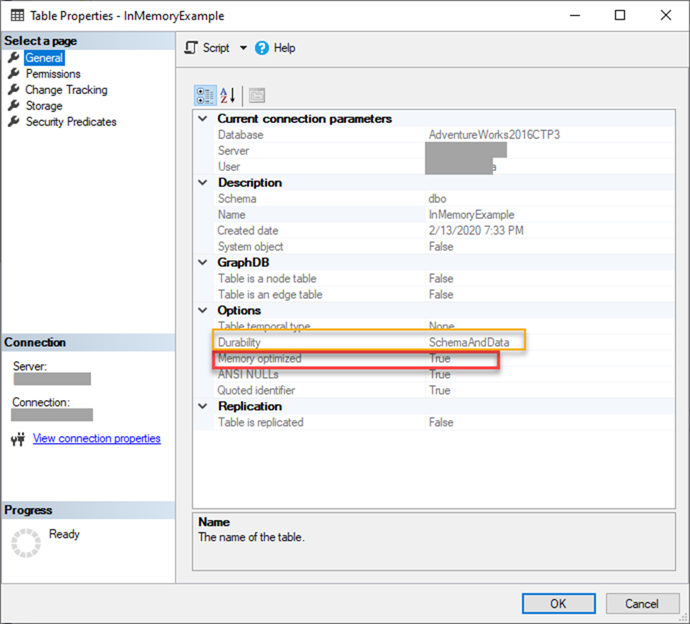
Table properties show Memory Optimized = TRUE and Durability = SchemaAndData once the table is created which makes it very simple to verify what the table is doing.

Inserting and selecting against the table is syntactically the same as any other regular table, however, internally it is far different. Above and beyond the table creation, its structured behavior is basically the same in these actions including adding or removing a column.  Now one caveat to these tables is that you cannot CREATE or DROP an Index the same way. You must use ADD/DROP Index to accomplish this, and, believe me, I tried. Indexing these tables is covered later in the article.

Remember the DURABILITY option I briefly mentioned before? This is important. The example above has it set to SCHEMA_AND_DATA which means, upon database going offline, both the schema and data are preserved on disk. If you choose SCHEMA_ONLY, this means that only the structure will be preserved, and data will be deleted. This is very important to note as it can introduce data loss when used incorrectly.

As you can see, In-Memory tables are not as complicated as my brain wanted to make them. It’s a relatively simple concept that just incorporates row versioning and two copies of the table. Once you pull the concept apart into its parts, it really makes it easier to understand.

Which Tables Do I Put In-Memory?

Determining which tables could benefit from being In-Memory is made easy by using a tool called Memory Optimization Advisor (MOA). This a is a tool built into SQL Server Management Studio (SSMS) that will inform you of which tables could benefit using In-Memory OLTP capabilities, and which may have non supported features. Once identified, MOA will help you to migrate that table and data to be optimized.

To see how it works, I’ll walk you through using it on a table I use for demonstrations in AdventureWorks2016CTP3. Since this is a smaller table and doesn’t incur a ton writes it is not a good use case, however, for simplicity I am using it for this demo.

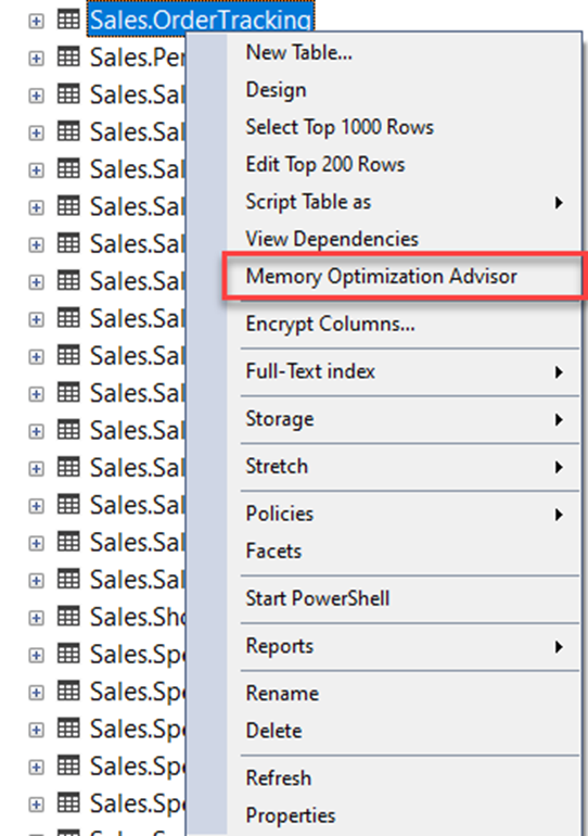
To get started, right-click on the Sales.OrderTracking table and select Memory Optimization Advisor.


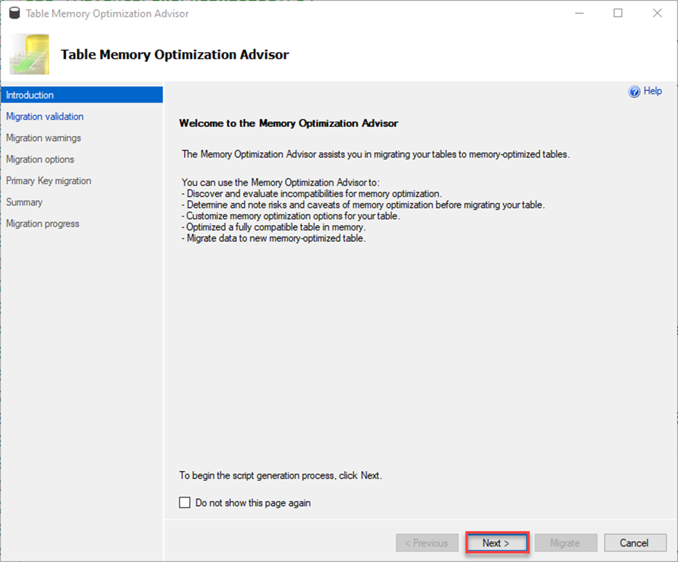
This brings up the wizard. Click Next to continue.

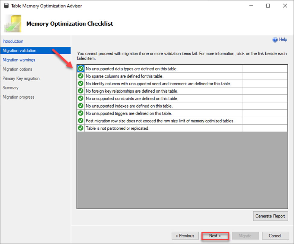
Next it will validate if your table is able to be migrated. It looks for things like unsupported data types, sparse columns, seeded columns, foreign keys, constraints and replication just to name a few. If any item fails, you must make changes and/or remove those features in order to move the table to a memory optimized table.

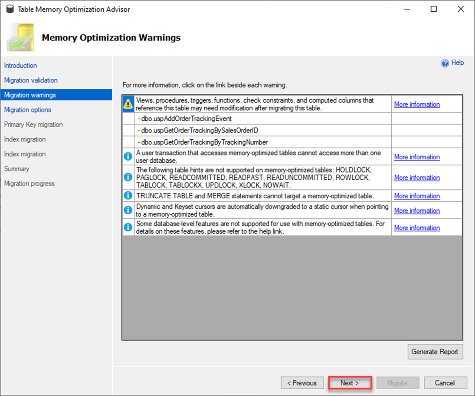
Next it will go over some warnings. These items, unlike the ones in the validation screen, won’t stop the migration process but can cause behavior of that option to fail or act abnormally so be aware of this. Microsoft goes a step further here and provides links to more information so that you can make an informed decision as whether or not to move forward with the migration.

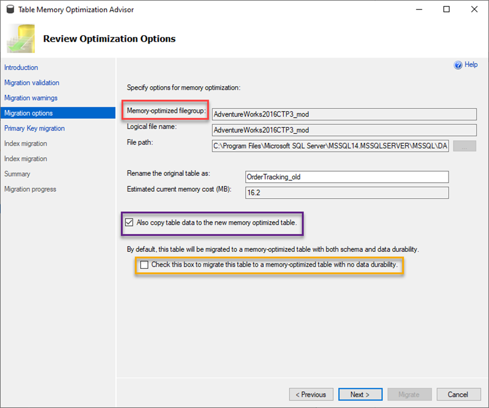
The next screen below is very important as it lets you choose options for your migration to a memory optimized table. I want to point out a few things in this next screen shot.

First, in the RED box, you will find requirement for a file group name. A memory optimized table must have a special file group when migrating. This is a requirement to allow you to rename the original table and keep it in place thus avoiding naming conflicts. You will note also in this screen that you can choose what to rename the original table.

Next in the PURPLE box, you will see the option to check to also have the data moved to the new table. If you do not check this option, your table will be created with no rows and you will have to manually move your data.

Next in the YELLOW box is the create table option that is equivalent to DURABILITY= SCHEMA_ONLY or SCHEMA_AND_DATA that I mentioned earlier in the article. If you do check this box, then you will not have any durability, and your data will disappear due to things like a restart of SQL Services or reboots (this may be what you want if you are using this table as though it was a TEMP TABLE and the data is not needed). Be very aware of these options because, by default, this is not checked. If you are not sure which option to choose, don’t check the box. That will ensure the data is durable. Click Next.

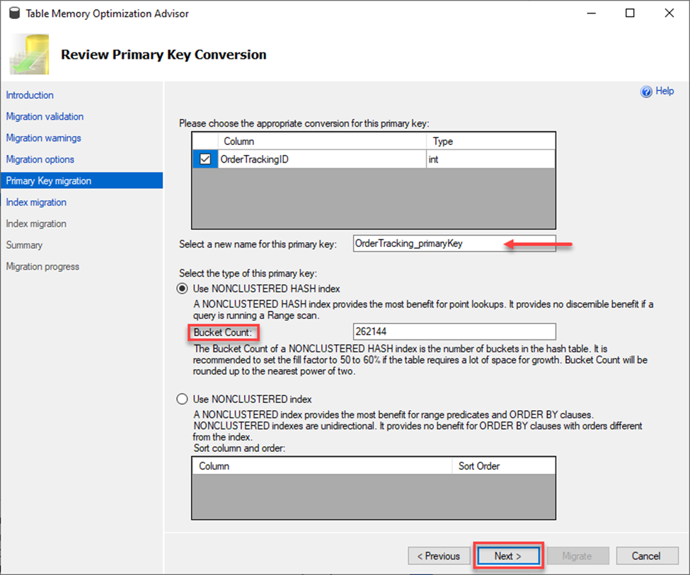
Remember that this is making a copy of your table for migration so the new optimized table cannot have the same primary key name. This next screen assists with renaming that key as well as setting up your index and bucket counts. I’ll explain bucket counts more below.

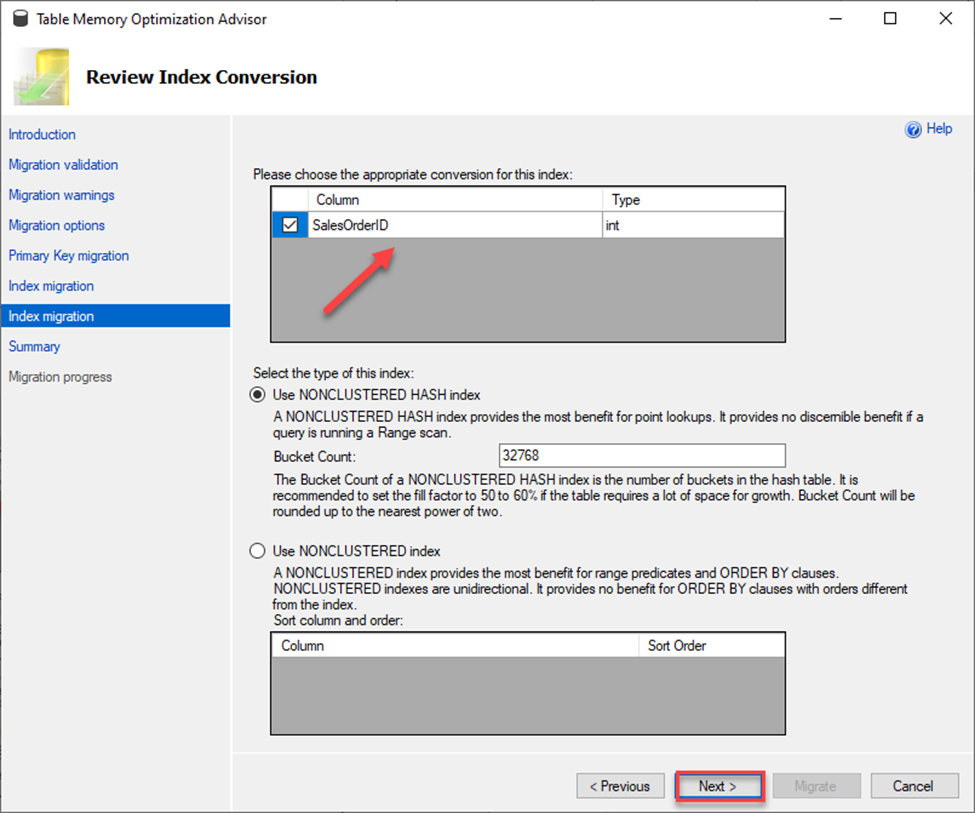
Note in the screen above it provides you a space to rename your primary key and create a new index. As you know, a primary key is an index so you must set that up. You have two options for the second index. You can use a NONCLUSTERED INDEX which is great for tables with many range queries and needing a sort order or you can use a NONCLUSTERED HASH index which is better for those direct lookups. If you choose the latter, you also need to provide a value for the Bucket Count. Bucket count can dramatically impact the performance of the table, and you should read the documentation on how to properly set this value. In the case above, I am leaving it to the pre-populated value and choosing Next.

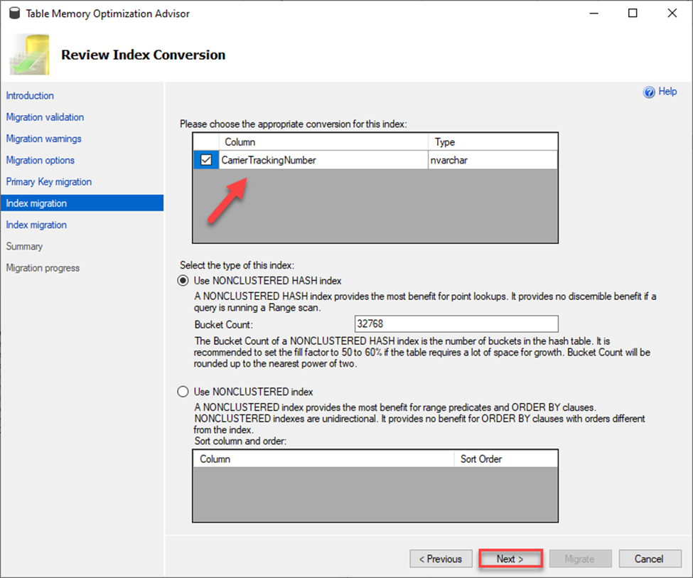
This table has existing indexes, so the next step is to run through the setup up of those for conversion. If you do not have any existing indexes this part is bypassed.

Note the two index migration options on the left. This means there are two indexes to migrate.

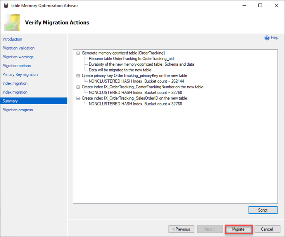
The next screen to come up is just a summary of all the migration options chosen in the setup. By choosing to migrate, you will migrate your table and its data to be an In-Memory optimized table so proceed with caution. This maybe a good time to hit the Script button and script this out for later use. Keep in mind that I already have a memory optimized file group for this database so one is not created for me. If one didn’t already exist,  you would see its creation in Summary screen.

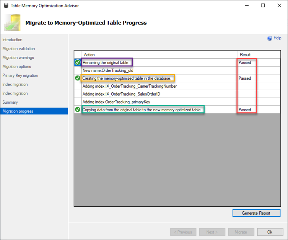
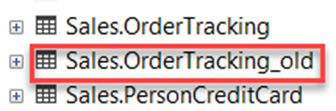
As shown below, the migration was successful. A new table was created while the old table was renamed, and the data was copied over.

Here are the results.


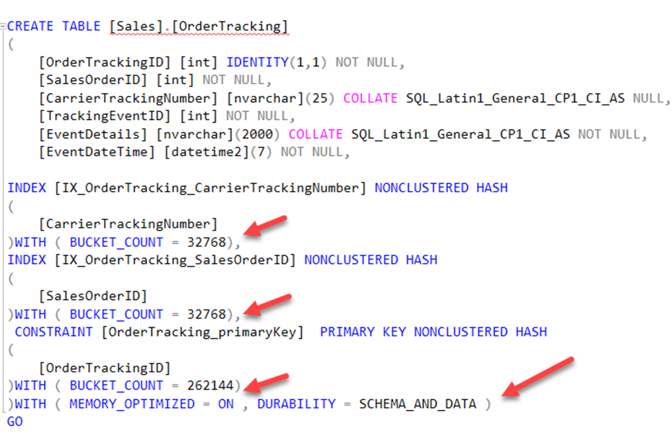
If I script out the new table now you will see that it notates it is a memory optimized table and has appropriate  bucket counts. Also note I DID NOT check the box that would have made my table SCHEMA_ONLY durable and you see that reflected with the DURABILTIY = SCHEMA_AND_DATA below.

As you can see the Memory Optimization Advisor makes it simple to identify and migrate tables to In-Memory Optimized Tables. I highly advise testing this process before trying to convert any tables in your databases. Not all workloads are viable candidates for this feature, so be sure to do your due diligence before implementation.  When you are ready to implement, this tool can help make that process a lot easier for you.

Now that I have explained about In-Memory Tables and Migrating to In-Memory tables, the next step is looking at indexes and how they are created and how they work within those tables. As you can imagine indexes, called memory optimized indexes are different for these types of tables, so take a look at just how different that are from regular tables.

Before diving into this subject, it is VERY important to note the biggest differences.

First, if you are running SQL Server 2014, memory optimized indexes MUST be created when the table is created or migrated. You cannot add indexes to an existing table without dropping and recreating the table. After 2016, you now have the option, and this limitation has been removed.

Secondly, prior to 2017 you could only have eight indexes per table including your primary key. Remember that every table must have a primary key to enforce a secondary copy for a minimum of schema durability. This  means you can only really add seven additional indexes so be sure to understand your workloads and plan indexing accordingly. Per Microsoft, starting with SQL Server 2017 (14.x) and in Azure SQL Database, there is no longer a limit on the number of indexes specific to memory-optimized tables and table types.

Third, Memory Optimized Indexes only exist in memory, they are not persisted to disk, and are not logged in the transaction logs. Therefore, this means they are also recreated upon database startup and do incur a performance hit as they are rebuilt.

Next, there is no such thing as key lookups against an In-Memory table, as all indexes are by nature a covering index. The index uses a pointer to the actual rows to get the needed fields instead of using a primary key like physical tables do. Therefore, these are much more efficient in returning the proper data.

Lastly, there also is no such thing as fragmentation for these indexes, since these are not read from disk. Unlike on disk indexes, these do not have a fixed page length. On disk indexes use physical page structures within the B-Tree, determining how much of the page should be filled is what the Fill Factor does. Since this is not a requirement, fragmentation does not exist.

Ok now that you made it through all of that, look at the types of indexes you can create and gain an understanding of what they are and how they are created.

Nonclustered HASH Indexes

This index is used to access the In-Memory version of the table, called a Hash. These are great for predicates that are singleton lookups and not ranges of values. These are optimized for seeks of equality values. For example, WHERE Name = ‘Joe’. Something to keep in mind when determining what to include in your indexes is this: if your query has two or more fields as your predicate and your index only consists of one of those fields, you will get a scan. It will not seek on that one field that was included. Understanding your workloads and indexing on the appropriate fields (or a combination thereof) is important. Given that this In-Memory OLTP is mainly focused on heavy insert/update workloads, and less so reading, this should be less of a concern.

These types of indexes are highly optimized and do not work very well if there are a lot of duplicate values in an index, the more unique your values better the index performance gains you will get. It is always important to know your data.

When it comes to these indexes, knowing your memory consumption plays a part. The hash index type is fixed length and consumes a fixed amount of memory determined upon creation. The amount of memory is determined by the Bucket Count value. It is extremely important to make sure this value is as accurate as possible. Right sizing this number can make or break your performance. Too low of a number, according to Microsoft, “can significantly impact workload performance and recovery time of a database.” Meanwhile, you can learn more about hash indexes at docs.microsoft.

Using T-SQL (both methods give the same result)

Example One (Note the index comes after the table fields)

CREATE TABLE [Sales] 
   ([ProductKey] INT NOT NULL,  
    [OrderDateKey] [int] NOT NULL,
   INDEX IDX_ProductKey HASH ([ProductKey]) WITH (BUCKET_COUNT = 100))  
   WITH (MEMORY_OPTIMIZED = ON, DURABILITY = SCHEMA_ONLY)
 

Example Two (Note the index comes after the field)

CREATE TABLE [Sales]  
   ([ProductKey] INT NOT NULL INDEX IDX_ProductKey HASH 
    WITH (BUCKET_COUNT = 100),
[OrderDateKey] [int] NOT NULL)  
   WITH (MEMORY_OPTIMIZED = ON, DURABILITY = SCHEMA_ONLY)


Nonclustered Indexes

Nonclustered indexes are also used to access the In-Memory version of the table however, these are optimized for range values such as less than and equal to, inequality predicates and sorts orders. Examples are WHERE DATE between ‘20190101’ and ‘20191231’ and WHERE DATE <> ‘20191231’. These indexes do not require a bucket count or fixed memory amount. The memory consumed by these indexes are determined by the actual row counts and size of the indexed key columns which makes it a simpler to create.

Moreover, in contrast to hash indexes which need all fields required for your predicate to be part of your index to get a seek, these do not. If your predicates have more than one field and your index has that one of those as its leading index key value, then you can still attain a seek.

Using T-SQL (both methods give the same result)

Example One (Note the index comes after the table fields)

CREATE TABLE [Sales] 
   ([ProductKey] INT NOT NULL,  
    [OrderDateKey] [int] NOT NULL,
   INDEX IDX_ProductKey ([ProductKey]))
   WITH (MEMORY_OPTIMIZED = ON, DURABILITY = SCHEMA_ONLY)

Example Two (Note the index comes after the field)

CREATE TABLE [Sales]  
   ([ProductKey] INT NOT NULL INDEX IDX_ProductKey,
    [OrderDateKey] [int] NOT NULL)  
   WITH (MEMORY_OPTIMIZED = ON, DURABILITY = SCHEMA_ONLY)

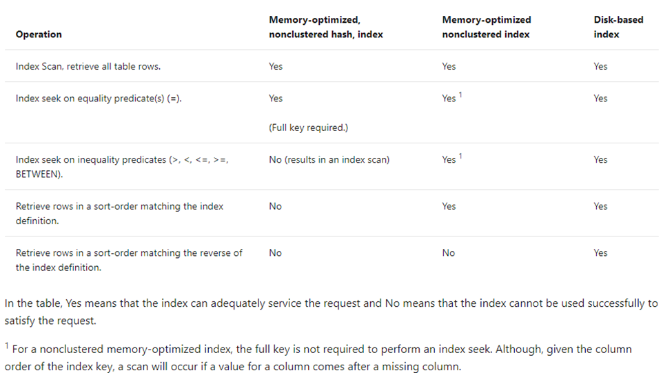
Determining which index type to use can be tricky but Microsoft has provided a great guide in the below chart.

Conclusion

As you can see there some key differences to how In- Memory table indexes, memory optimized indexes, work compared to the normal disk indexes. Like with any other table design it is important to consider your index needs before you embark on creating or migrating to memory optimized tables. You’ll be happy you did.

The post Beginner Guide to In-Memory Optimized Tables in SQL Server appeared first on Simple Talk.


from Simple Talk https://ift.tt/2Hr7oAy
via

Friday, February 14, 2020

Creating Time-Intelligence Functions in DAX

The series so far:

  1. Creating Calculated Columns Using DAX
  2. Creating Measures Using DAX
  3. Using the DAX Calculate and Values Functions
  4. Using the FILTER Function in DAX
  5. Cracking DAX – the EARLIER and RANKX Functions
  6. Using Calendars and Dates in Power BI
  7. Creating Time-Intelligence Functions in DAX

Want to compare this year’s sales with the same period in the previous year? Chart year-to-date costs? Or perhaps you want to create a twelve-month moving average of profitability? In the last article in this series, you’ll learn how to use the time-intelligence functions built into DAX and understand why they work.

Loading the Sample Data for this Article

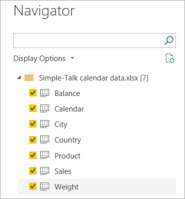
To work through the examples in this article, you’ll need to download the worksheets from this workbook. Tick the following worksheets to load data from this workbook into a new Power BI report:

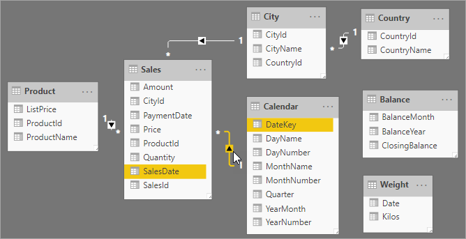
Now create a relationship between the Calendar and Sales tables by the SalesDate column, as follows (note that initially the Balance and Weight tables aren’t linked to any others):

NOTE: This article assumes that you are only concerned with the date when sales are made. If you wanted to be able to choose between the sales date and the payment date when analysing data, you’d either have to create multiple versions of the Calendar table or multiple relationships, as described in the previous article in this series.

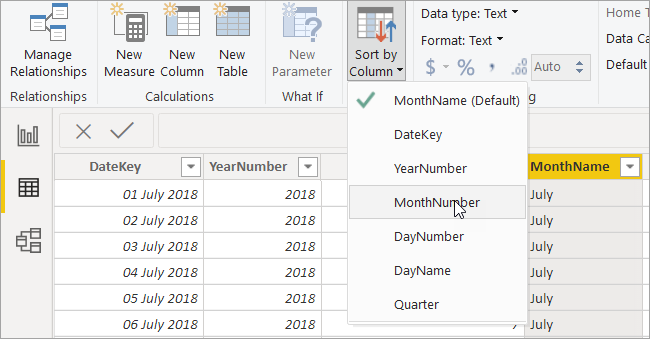
Finally, switch to the Modeling ribbon and choose to sort the month name by the month number:

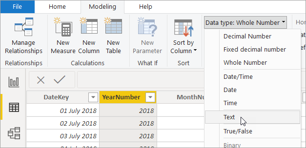
And make the YearNumber a text column:

Again, the reason for both of these changes is covered in the previous article in this series.

Creating a Draft Matrix

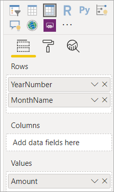
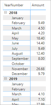
To accommodate all the wonderful measures that you’re going to bring into being, create a matrix visual to show total amount sold by year and month:

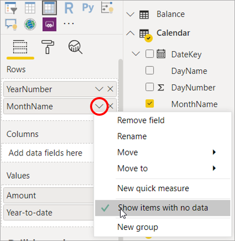
I think it’ll be easier to work with if you have all 12 months appearing, so choose to show months even when they have no corresponding data:

Here’s what the start of the matrix should look like:

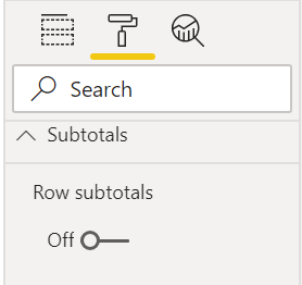
I’ve decided to hide the row subtotals for the matrix. To turn these off, go to the formatting tab and look under the Subtotals section for Row subtotals.

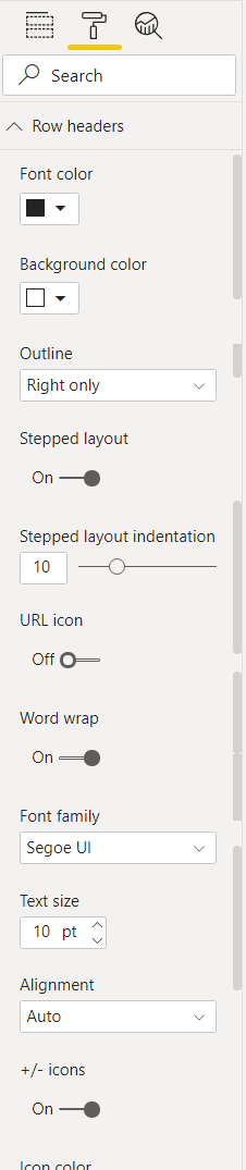
If for any reason you don’t get the +/- icons to expand/collapse rows, enable this setting in the matrix’s formatting properties:

How Time-intelligence Functions Work

To begin with, create a new measure on the Sales table to show total sales to date for each year (don’t worry too much yet about how this works):

Year-to-date = CALCULATE(
    SUM(Sales[Amount]),
    DATESYTD('Calendar'[DateKey])
)

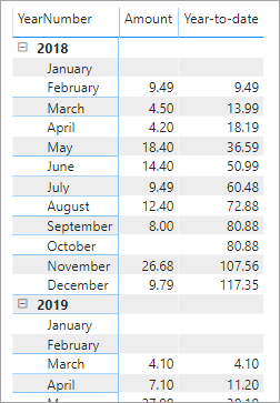
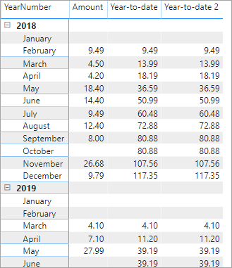
I’ll come back to the DATESYTD function in more detail later in this article, but for the moment I want to use it as an example to explain how any DAX time-intelligence function is calculated. Here’s what this measure should show for the matrix:

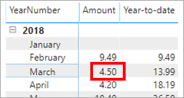
What I want to do is to focus on one figure – the year-to-date sales for March 2018. Start by looking at the sales amount for March 2018, which is 4.50:

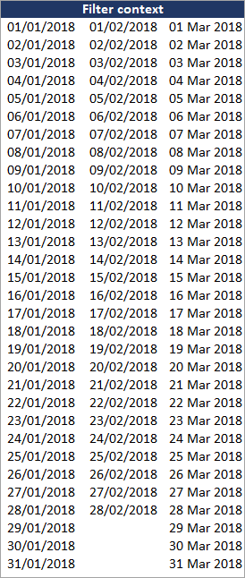
The filter context for this figure is all of the dates in March 2018:

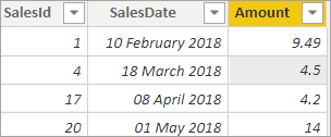
There’s only one sale in March 2018, so that’s why you get 4.50 as the sales for the cell:

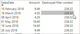
By contrast, the measure to calculate year-to-date sales first destroys the existing filter context for the sales date. Without any additional change, you would get the same figure for each month:

However, the measure then replaces the filter context with one which picks out all of the dates from the calendar table which are on or before 31st March in 2018:

Year-to-date = CALCULATE(
    SUM(Sales[Amount]),
    DATESYTD('Calendar'[DateKey])
)

The filter context is now as follows for the cell:

Power BI knows when days, months, quarters, and years start and end (they’re called time-intelligence functions for a reason!). Curiously, Power BI doesn’t know about weeks, so if you want to do weekly reporting, you’ll have to create new aggregator columns yourself in your calendar table (again, the previous article in this series gives a guide for how to do this sort of thing).

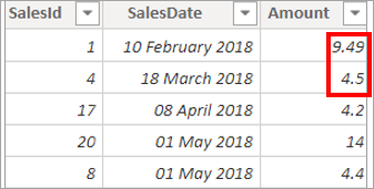
Here are the sales figures for the start of 2018:

Adding 9.49 and 4.5 gives the year-to-date figure of 13.99! This is what every time-intelligence function does: it destroys the previous filter context for each value in a visual’s underlying data and replaces it with a different one according to the combination of DAX functions you’ve chosen.

Period to Date Functions

Now to take a look in detail now at how to do specific things, beginning with calculating yearly, quarterly or monthly cumulative figures. You can do this using one of these functions:

  • DATESYTD or TOTALYTD (year-to-date)
  • DATESQTD or TOTALQTD (quarter-to-date)
  • DATESMTD or TOTALMTD (month-to-date)

This functionality is typical of time-intelligence functions in DAX: there are often two or three ways to do the same thing, and which one you use is a matter of personal preference. Here’s a function giving the year-to-date figures using DATESYTD shown earlier:

Year-to-date = CALCULATE(
    // you could use a different aggregation function
    SUM(Sales[Amount]),
    // calculate over the dates for the year-to-date
    DATESYTD('Calendar'[DateKey])
)

Here’s a function to do exactly the same thing using TOTALYTD:

Year-to-date 2 = TOTALYTD(
    // again, we could use MAX, MIN, COUNT, etc. here
    SUM(Sales[Amount]),
    'Calendar'[DateKey]
)

These two measures should give the same figures because they are, after all, doing exactly the same thing:

I prefer the first measure since it’s clearer what it’s doing (destroying the existing filter context, and replacing it with one which uses the dates for the current year up to and including the last day in the current period). The second measure using TOTALYTD is just a convenient shorthand for this.

Coping with Different Financial Year-ends

Not everyone’s financial years end conveniently on 31st December, so you can specify a second argument for the DATESYTD function, giving your year-end date in the format DD-MM:

As an example, suppose that your year ends on 31st March. Then you could use this measure:

Year-to-date = CALCULATE(
    // you could use a different aggregation function
    SUM(Sales[Amount]),
    // calculate over the dates for the year-to-date,
    // but with year ending on 31st March
    DATESYTD('Calendar'[DateKey],"31-03")   
)

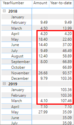
This measure would give this report (the box shows how the figures from 1st April 2018 to 31st March 2019 are calculated):

This result would look much better if you created a new aggregator column to give the financial year and reported by that. An idea of how to do this is shown in the previous article in this series. Since I’m feeling charitable, here is the formula that you could use to create a new calculated column in your Calendar table for the financial year:

Financial year = IF(
    [MonthNumber] <= 3,
    // for dates up to and the end of March
    [YearNumber] - 1 & "-" & [YearNumber],
    // for dates from April to December
    [YearNumber] & "-" & [YearNumber] + 1
)

You’ll also need a formula to determine how to sort months, so that April comes first and March last:

Financial month sort order = IF(
    [MonthNumber] <= 3,
    // for dates up to and the end of March
    [MonthNumber]+12,
    // for dates from April to December
    [MonthNumber]
)

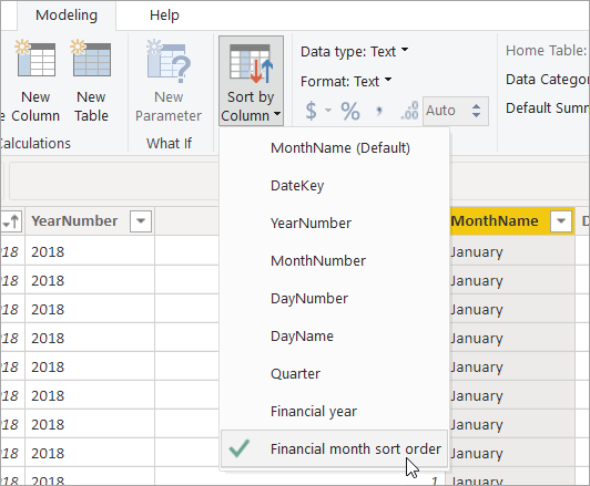
You can then choose to sort your months by the Financial month sort order column you’ve created:

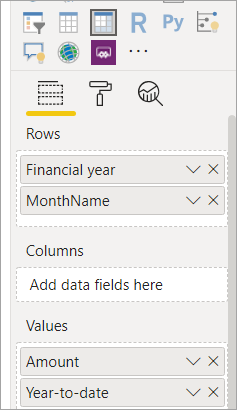
If you then display the financial year column you’ve created in your matrix instead of the year, like this:

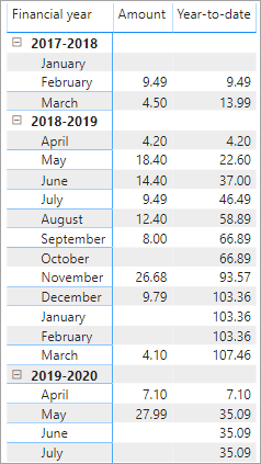
You should now get something a lot less confusing:

This may seem like a lot of faff, but remember that you’ll only have to set up the calculated columns in your calendar once and once only.

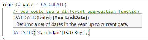
Finally, on the subject of changing your year-end dates, I’ve only shown so far how to change the financial year-end using the DATESYTD function. The process for the TOTALYTD function is similar, but there is a catch. Here’s the syntax:

So it looks for all the world as if the argument to set a new year-end date is the fourth one, and that if you’re not setting any additional filter, you will need to find some way to omit the third argument. However, this measure works:

Year-to-date 2 = TOTALYTD(
    // again, we could use MAX, MIN, COUNT, etc. here
    SUM(Sales[Amount]),
    'Calendar'[DateKey],
    // change the year-end date
    "03-31"
)

Somehow Power BI works out that you’ve missed out the third Filter argument. In every other Microsoft product I’ve used, you need to use a comma placeholder to show that you’re omitting an argument to a function, but if you try to do this in the formula above you get an error!

If you’re wondering which functions support the additional year-end argument, the answer is all those for which this would be relevant – here’s the list for reference:

Functions

What they do

STARTOFYEAR, ENDOFYEAR

Return the first or last date in the year for the current filter context.

PREVIOUSYEAR, NEXTYEAR

Return a table of the dates in the previous or next year, based on the current filter context’s latest date.

DATESYTD, TOTALYTD

As covered on the previous page!

OPENINGBALANCEYEAR, CLOSINGBALANCEYEAR

Return the opening or closing balance on the first/last day of the year for the current filter context.

Referencing Previous Periods

Suppose that you want to show for each day, month, quarter or year what your sales were in the same period twelve months ago? Again, there are two ways (at least) to do this:

  • Using the DATEADD function
  • Using the SAMEPERIODLASTYEAR function

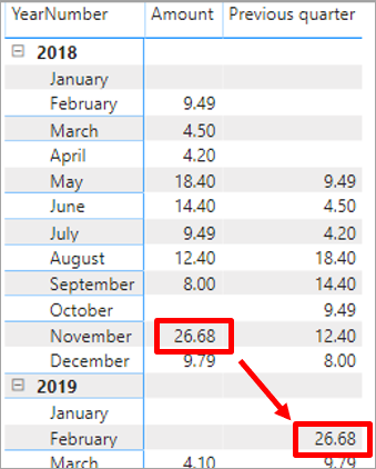
The DATEADD function is more useful, as it can also show sales 13 months ago, or four years ago or indeed any number of periods of any type ago, but I’ll explain both functions in the interest of fairness. Start by showing for each month the sales in that month against the sales in the same month in the previous quarter, which should give this:

Note that I’ve reverted to using the typical calendar month and year in the matrix, and I’m sorting the calendar months by the MonthNumber column again.

So, for example, the measure should show previous quarter sales for February 2019 as 26.68, since these were what the sales were three months earlier for the same period. You can’t use the SAMEPERIODLASTYEAR function to do this for obvious reasons (the clue’s in the name), and for some strange reason there isn’t an equivalent SAMEPERIODLASTMONTH or SAMEPERIODLASTQUARTER function, so instead, you’ll use the versatile DATEADD function. This takes three arguments:

The arguments are:

  1. The calendar dates, as usual
  2. The number of intervals to go forward in time
  3. The interval to use

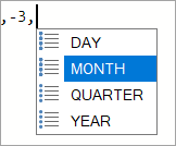
Here’s what you’ll see for the third argument when typing it in:

For this example, you can either go three months back in time or one quarter; it makes no difference which you choose. I’ve gone for three months, to produce this measure:

Previous quarter = CALCULATE(
    SUM(Sales[Amount]),
    // go back 3 months (could have used -1 QUARTER)
    DATEADD('Calendar'[DateKey],-3,MONTH)
)

Since the DATEADD function is so powerful (you can go forward or backwards in time, using days, months, quarters or years as the time interval), it seems pointless having the SAMEPERIODLASTYEAR function as a shortcut for it. Nevertheless, it exists! To illustrate it, switch to showing for each period what sales were 12 months (i.e. one year) previously. You could solve this using this measure:

Previous year 1 = CALCULATE(
    SUM(Sales[Amount]),
    SAMEPERIODLASTYEAR('Calendar'[DateKey])
)

Or this measure:

Previous year 2 = CALCULATE(
    SUM(Sales[Amount]),
    DATEADD('Calendar'[DateKey],-1,YEAR)
)

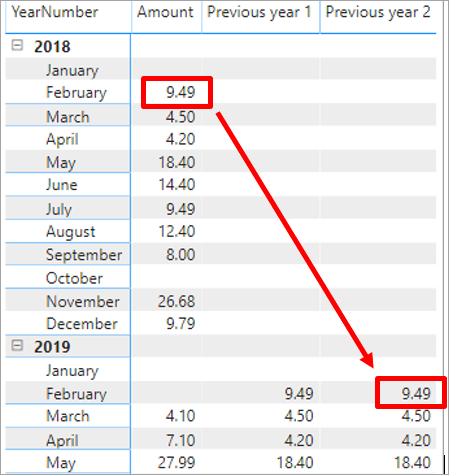
To prove this, here are both measures in the matrix, showing that they both return 9.49 against February 2019, since that’s what sales were for the corresponding period 12 months previously:

Getting the Whole of a Previous Period

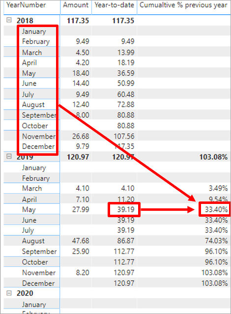
The functions above return a figure for a corresponding period, but what happens if you want to get sales for the whole of the previous period? To see what this means, consider this example (it shows year-to-date figures as a fraction of total sales for the whole of the previous year):

The figure shown for May 2019 (boxed above) is 33.40%, since year-to-date sales at this point are 39.19, and sales for the whole of the previous 12-month period were 117.35. 39.19 divided by 17.35 gives 33.40%. The fact that by the end of 2019, the sales have exceeded 100% of the sales for the whole of the previous year is presumably a good sign!

To calculate this measure, use the PARALLELPERIOD function. This has the same format as the DATEADD function but returns the aggregate figure for the whole of a previous period, rather than for the period corresponding to the one you’re viewing. The syntax of the function is as follows:

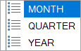
The interval can be any one of the following:

Note that unlike for the DATEADD function you can’t use the PARALLELPERIOD function to return the aggregate of a number for the whole of the previous day, presumably because this is at too low a level of granularity.

Putting all this together, here’s how the measure to give the figures above might read:

Cumulative % previous year = DIVIDE(
    // divide the year-to-date figure …
    CALCULATE(
        SUM(Sales[Amount]),
        DATESYTD('Calendar'[DateKey])
    ),
    // … by sales for the whole of the previous year
    CALCULATE(
        SUM(Sales[Amount]),
        PARALLELPERIOD('Calendar'[DateKey],-1,YEAR)
    )
)

That is: divide year-to-date sales by sales for the whole of the previous year.

To format the measure, select it in the list of fields. Then, on the Modeling ribbon, format as a percentage with two decimal places.

Moving Averages

Moving averages are one of the most useful ways to show trends, since they iron out any seasonal effects. Sadly, there is no MOVINGAVERAGE function in DAX, but you can create your own expression in a couple of different ways, of which I’ve shown the one I believe to be the more useful below.

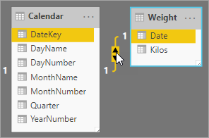
To illustrate moving averages, first create a relationship between the Weight and the Calendar tables:

The Weight table is a bit of an anomaly – it doesn’t have anything to do with the others. I’ve been recording my weight roughly every week for the last couple of years, to see if it’s going up or down. Although this is slightly obsessive behaviour, it does provide a perfect example of the use of moving averages.

Add a calculated column to the Calendar table:

The new column should use this formula:

YearMonth = [YearNumber] &"-"& if([MonthNumber]<10,"0","") 
    & [MonthNumber]

This column should return the year number and month number for each calendar date, which you can then use to display as labels on a chart:

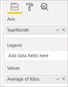
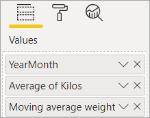
Now create a line chart showing the average of the Kilos field from the Weight table against the YearMonth field from the Calendar table:

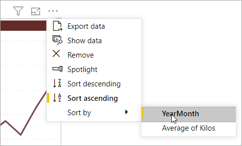
Make sure that you choose to show the average kilos, not the default sum. Also, you will need to sort your chart by the YearMonth field, not by the average kilos (the default):

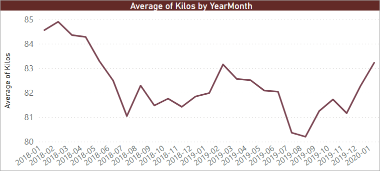
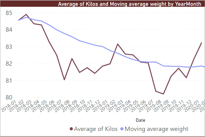
You should get something like this (I’ve formatted my chart a bit, but it’s the underlying trend which interests us here):

The question is this – is my weight going up or down? To answer this, you have to take account of seasonality –I eat way too much at Christmas but tend to go on family cycling holidays in July during which my weight falls. To show what’s happening, create a 12-month moving average. If this works, the figure for February 2019, for example, should return the average for the previous 12 months (that is for the period March 2018 through to February 2019).

Here’s a measure you could create to show the 12-month moving average:

Moving average weight = CALCULATE(
    -- average weight in kilos ...
    AVERAGE('Weight'[Kilos]),
    
    -- ... over the period between two dates, 
    -- as specified in the arguments
    DATESBETWEEN(
        'Calendar'[DateKey],
        
        -- the first date takes the last date
        -- for the filter context, works out
        -- what the corresponding period would 
        -- have been for the previous year and 
        -- adds one day to the last date of it
        NEXTDAY(
            SAMEPERIODLASTYEAR(
                LASTDATE('Calendar'[DateKey])
            )
        ),
        
        -- the last date is just the end date
        -- for the filter context
        LASTDATE('Calendar'[DateKey])
    )
)

Here’s the chart this would give, and it looks like good news – my weight may be going up and down, but on a seasonally adjusted basis it’s falling steadily, if slowly:

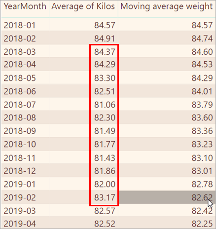
To understand how the measure works, create a table to include these fields:

This table should show the following data (I’ve added the red box separately – you obviously won’t be able to create this in Power BI):

The 12-month moving average for February 2019 is 82.62 and is shown selected above. This is the average of the figures for the 12 months shown in the red box. To see how the measure arrives at this figure, start in the middle of it:

LASTDATE('Calendar'[DateKey]

This expression would return 28th February 2019 for the above example (being the last date in the date filter context period for the month under consideration). Now add the next bit of the measure:

SAMEPERIODLASTYEAR(
    LASTDATE('Calendar'[DateKey])
)

This expression will give 28h February 2018, being the corresponding date in the previous calendar year. Expand the measure a bit more and you get:

NEXTDAY(
SAMEPERIODLASTYEAR(
     LASTDATE('Calendar'[DateKey])
)
)

This expression will give the day following 28th February 2018 (that is, 1st March 2018). So the whole date range across which you’re averaging my weight is given by:

DATESBETWEEN(
        'Calendar'[DateKey],
        
        -- the first date takes the last date
        -- for the filter context, works out
        -- what the corresponding period would 
        -- have been for the previous year and 
        -- adds one day to the last date of it
        NEXTDAY(
            SAMEPERIODLASTYEAR(
                LASTDATE('Calendar'[DateKey])
            )
        ),
        
        -- the last date is just the end date
        -- for the filter context
        LASTDATE('Calendar'[DateKey])
    )

This gives the dates between 1st March 2018 and 28th February 2019, which was the goal!

Semi-additive Measures

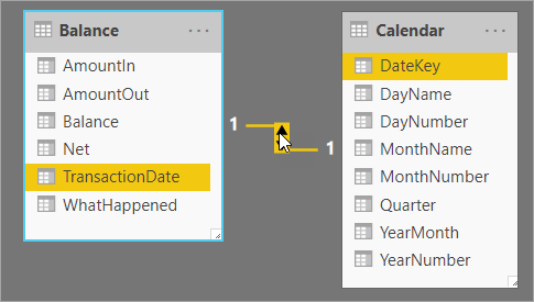
For the last part of this tutorial on using time-intelligence functions, I’ll discuss semi-additive measures (that is, measures which sometimes aggregate data and sometimes don’t). To start, create a new layout in your report, and create this relationship:

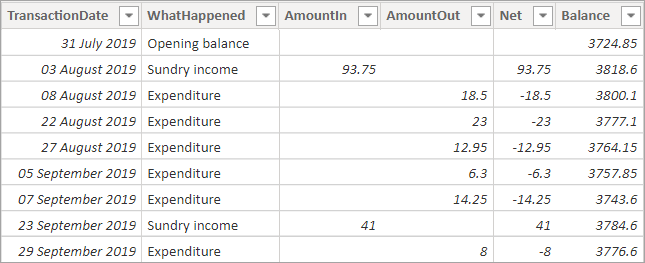
Suppose that the Balance table contains your bank statement for the period July to September 2019. You want to get the closing bank balance at the end of each month, so you create a report based on this Balance table:

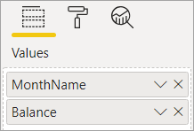
To do this, you add a table with these fields:

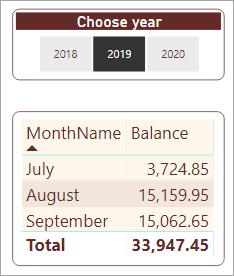
You should now see this table (if you include a slicer as shown to look at 2019 data only):

This result is clearly wrong (it would be nice if your bank added your daily balances to get your monthly balance, assuming that you aren’t overdrawn, but life doesn’t work that way). The goal is to pick out the last amount in each month. Fortunately, there is a family of semi-additive DAX functions to draw on:

Function(s)

What the functions do

CLOSINGBALANCEYEAR, CLOSINGBALANCEQUARTER, CLOSINGBALANCEMONTH, OPENINGBALANCEYEAR, OPENINGBALANCEQUARTER, OPENINGBALANCEMONTH

Calculate the value of an expression at the first or last date of the year, quarter or month for the current filter context.

FIRSTDATE, LASTDATE

Return the first or last date for the filter context.

FIRSTNONBLANK, LASTNONBLANK

Return the first or last date for the filter context for which a given expression has a value.

For this example, you could try using the LASTDATE function, with this measure:

Attempt at closing balance = CALCULATE(
    -- work out the total balance ...
    SUM(Balance[Balance]),
    
    -- for the last date in the current
    -- filter context
    LASTDATE('Calendar'[DateKey])
    
)

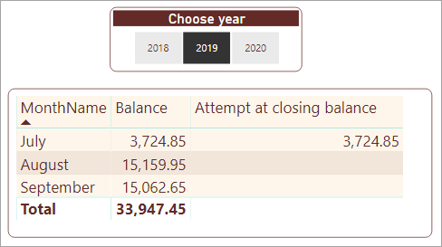
This formula would give this column in the table:

This formula is a bit better, but it only shows figures for July. This is because in the table of balances, there weren’t any transactions on the last dates of August or September in 2019, so the measure is returning blank for these two months. You could get around this by using the clever LASTNONBLANK function, which will return the balance on the last date for which a transaction exists:

Closing balance = CALCULATE(
    // work out the total balance ...
    SUM(Balance[Balance]),
    
    LASTNONBLANK(
    
        // ... for the last date in the current filter context ...
        'Calendar'[DateKey],
        
        // ... for which there are rows in the table of balances
        COUNTROWS(RELATEDTABLE(Balance))
    )   
)

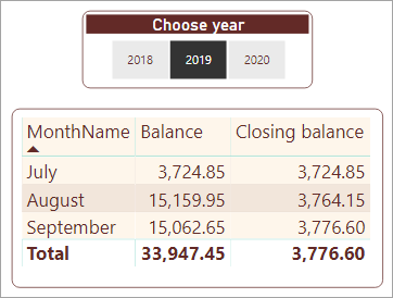
This measure will give the correct closing balances. The function is called semi-additive because you could then aggregate these if you chose, although normally you won’t want to do this:

The measure needs a bit of explanation. The syntax of the LASTNONBLANK function is as follows:

The measure returns the total balance for each month on the last day for which there are any corresponding rows in the Balance table. The reason for the RELATEDTABLE function is that at this point in the measure it’s slipped from filter to row context. The LASTNONBLANK function is an iterator function which goes down the rows in the current filter context (for this example, the dates in each month), evaluating for each whether it could be included. Relationships between tables aren’t automatically supported within row context, so you need to use the RELATEDTABLE to bring information in from another table.

It seems appropriate to end with this paragraph about row and filter context, since understanding these two concepts is key to understanding DAX. Thank you for reading through this article, and (perhaps) the other ones in this series, and happy DAXingthe date of the sale If you’ve enjoyed the series, you may like to know that the author’s company Wise Owl Training provide classroom training in Power BI and DAX, although currently only in the UK.

Conclusion

In this article, you’ve learnt that you can override the default filter context for any measure referencing a calendar date column. The replacement filter context could, for example, allow you to return year-to-date figures, show data from the same period in a previous month, quarter or year, or even show totals from prior periods or moving averages. You’ve also learnt how to use semi-additive measures to show closing (and by analogy) opening balances. You should also now have a feel for the fact that time-intelligence functions have this name because DAX has built-in knowledge of how days, months, quarters and years behave.


The post Creating Time-Intelligence Functions in DAX appeared first on Simple Talk.


from Simple Talk https://ift.tt/37qjncf
via