Thursday, November 29, 2018

Power BI Introduction: Visualizing SQL Server Audit Data — Part 9

The series so far:

  1. Power BI Introduction: Tour of Power BI — Part 1
  2. Power BI Introduction: Working with Power BI Desktop — Part 2
  3. Power BI Introduction: Working with R Scripts in Power BI Desktop — Part 3
  4. Power BI Introduction: Working with Parameters in Power BI Desktop — Part 4
  5. Power BI Introduction: Working with SQL Server data in Power BI Desktop — Part 5
  6. Power BI Introduction: Power Query M Formula Language in Power BI Desktop — Part 6
  7. Power BI Introduction: Building Reports in Power BI Desktop — Part 7
  8. Power BI Introduction: Publishing Reports to the Power BI Service — Part 8
  9. Power BI Introduction: Visualizing SQL Server Audit Data — Part 9

Database teams trying to comply with regulations such as the Health Insurance Portability and Accountability Act of 1996 (HIPAA) or the Sarbanes-Oxley Act of 2002 (SOX) commonly use auditing as part of their compliance strategies to help track potential threats to stored data. For example, teams running SQL Server might turn to SQL Server Audit to log actions at both the server and database levels. SQL Server Audit is built into the database engine and, starting with SQL Server 2016, is available in all SQL Server editions.

If you’re a DBA tasked with implementing SQL Server Audit, you’ll find that setting up the auditing components is a relatively straightforward process. The more significant challenges often lie in trying to determine what user actions to audit, how to handle the potentially large amounts of audit data, and what tools to use to monitor and review that data.

Although these are all important considerations, this article is concerned primarily with the last one—monitoring and reviewing the audit data. SQL Server makes it easy to collect the data but provides no mechanisms for working with that data in a meaningful way, other than to review it manually.

One way to address this issue is to bring in a third-party solution such as EventTracker to consolidate, manage, and monitor the audit data, but this comes with additional licensing and implementation considerations.

Another approach is to use Power BI to create reports that provide quick visual insights into the data. Although Power BI is not designed for auditing and alerting to the same degree as more robust log management tools, it provides a relatively simple method for tracking user behavior. Best of all, the basic Power BI service is free, as is Power BI Desktop, a downloadable tool for transforming and visualizing different types of data.

In this article, I demonstrate how you can use Power BI to work with SQL Server Audit data, walking you through the steps necessary to set up a test environment, generate sample audit data, pull that data into Power BI Desktop, and create a report that contains tables and visualizations. Keep in mind, however, that SQL Server Audit and Power BI Desktop are both powerful solutions that support far more capabilities than can be covered in a single article. The information here should at least provide you with a conceptual overview of how the tools can be used together and what it takes to get started using Power BI Desktop to review audit data.

Setting Up a Test Environment

To prepare your environment for the examples in this article, you should first create the ImportSales test database, which contains one schema, Sales, and one table, Sales.Customers. You can then populate the table with data from the Sales.Customers table in the WideWorldImporters database. For this article, all audited actions are limited to Customers table in the ImportSales database.

To create the ImportSales database, run the following T-SQL code:

USE master;
GO
DROP DATABASE IF EXISTS ImportSales;
GO
CREATE DATABASE ImportSales;
GO
USE ImportSales;
GO
CREATE SCHEMA Sales;
GO
CREATE TABLE Sales.Customers(
  CustID INT IDENTITY PRIMARY KEY,
  Customer NVARCHAR(100) NOT NULL,
  Contact NVARCHAR(50) NOT NULL,
  Email NVARCHAR(256) NULL,
  Phone NVARCHAR(20) NULL,
  Category NVARCHAR(50) NOT NULL);
GO
INSERT INTO Sales.Customers(Customer, Contact, Email, Phone, Category) 
SELECT c.CustomerName, p.FullName, p.EmailAddress,
  p.PhoneNumber, cc.CustomerCategoryName
FROM WideWorldImporters.Sales.Customers c
  INNER JOIN WideWorldImporters.Application.People p
    ON c.PrimaryContactPersonID = p.PersonID
  INNER JOIN WideWorldImporters.Sales.CustomerCategories cc
    ON c.CustomerCategoryID = cc.CustomerCategoryID;
GO

If you don’t have the WideWorldImporters database installed, you can populate the Customers table with your own data. If you want to use a different table and database for these examples, skip the T-SQL statements above and use a database and table that best suit your needs (and are not in a production environment, of course). Just be sure to replace any references to the ImportSales database or Customers table in the subsequent examples.

The next step is to create an audit object at the SQL Server instance level and a database audit specification at the ImportSales database level. The audit object serves as a container for organizing the server and database audit settings and for delivering the final audit logs. For this article, you’ll be saving the audit data to a local folder, but know that SQL Server Audit also lets you save the data to the Windows Application log or Security log.

A database audit specification is created at the database level and is associated with an audit object, which means that the audit object needs to exist before you can create the database audit specification. The specification determines what actions should be audited at the database level. You can also create a server audit specification for auditing actions at the server level, but for this article, you need only the database audit specification.

To create both the audit object and database audit specification, run the following T-SQL code:

USE master;  
GO  
CREATE SERVER AUDIT ImportSalesAudit  
TO FILE (FILEPATH = 'C:\DataFiles\audit\');  
GO  
ALTER SERVER AUDIT ImportSalesAudit  
WITH (STATE = ON);  
GO  
USE ImportSales;  
GO  
CREATE DATABASE AUDIT SPECIFICATION ImportSalesDbSpec 
FOR SERVER AUDIT ImportSalesAudit
ADD (SCHEMA_OBJECT_CHANGE_GROUP),
ADD (SELECT, INSERT, UPDATE, DELETE 
  ON Object::Sales.Customers BY public)  
WITH (STATE = ON);  
GO

The CREATE SERVER AUDIT statement creates an audit object named ImportSalesAudit that saves the audit data to the C:\DataFiles\Audit folder. You must then run an ALTER SERVER AUDIT statement as a separate step to set the STATE property to ON.

Next comes the CREATE DATABASE AUDIT SPECIFICATION statement, which defines a specification named ImportSalesDbSpec. The specification includes two ADD clauses. The first ADD clause specifies the action group SCHEMA_OBJECT_CHANGE_GROUP, which audits all CREATE, ALTER, and DROP statements issued against any schema objects in the database. Because this is a group action, it must be specified separately from individual actions, such as those in the second ADD clause.

The second ADD clause specifies four individual actions:

  • The SELECT action audits all SELECT statements.
  • The INSERT action audits all INSERT statements.
  • The UPDATE action audits all UPDATE statements.
  • The DELETE action audits all DELETE statements.

The ON subclause in the second ADD clause points to the Customers table, which means that the SELECT, INSERT, UPDATE, and DELETE actions are all specific to that table. In addition, because the BY subclause specifies the public login, the auditing applies to all users.

Under normal circumstances, you would likely be auditing many more users and actions than you’ve done here, but this is enough to demonstrate the basic principles behind using Power BI to review audit data.

With the auditing structure in place, run the following T-SQL code to create three test user accounts within the ImportSales database, assigning a different set of permissions to each user:

CREATE USER User01 WITHOUT LOGIN;
GRANT ALTER, SELECT, INSERT, DELETE, UPDATE
ON OBJECT::Sales.Customers TO user01;  
GO
CREATE USER User02 WITHOUT LOGIN;
GRANT SELECT, INSERT, DELETE, UPDATE
ON OBJECT::Sales.Customers TO user02;  
GO
CREATE USER User03 WITHOUT LOGIN;
GRANT SELECT
ON OBJECT::Sales.Customers TO user03;  
GO

The user accounts are created without logins to keep the testing simple. For the same reason, all the granted permissions are specific to the Customers table, with access defined as follows:

  • User01 can access and modify all data within the table as well as update the table’s definition.
  • User02 can access and modify all data within the table but is not permitted to update the table’s definition.
  • User03 can access all data within the table but is not permitted to modify any of the data or update the table’s definition.

You can set up the test users and their permissions any way you like, so that you have them in place when you’re ready to generate audit data to use in Power BI Desktop.

Generating Test Audit Data

To generate the audit data, you should run a series of data manipulation language (DML) statements and data definition language (DDL) statements against the Customers table, running them within the execution context of the three database user accounts. The easiest way to do this is to use an EXECUTE AS statement to specify the user context, run one or more statements, and then run a REVERT statement to switch back to the original user.

You can run whatever DML and DDL statements you want, as long as you test each account and the permissions assigned to that account. On my system, I ran several sets of T-SQL statements, most of them multiple times to generate a reasonable amount of data. If you want to use the same statements that I used, start with the following DML statements, running them under the User01 account:

EXECUTE AS USER = 'User01';
SELECT * FROM Sales.Customers;
INSERT INTO Sales.Customers 
  (Customer, Contact, Email, Phone, Category)
  VALUES('Wingtip Toys (Eugene, OR)', 'Flora Olofsson', 
    'flora@wingtiptoys.com', '(787) 555-0100', 'Gift Store');
DECLARE @LastID INT = (SELECT SCOPE_IDENTITY())
UPDATE Sales.Customers SET Category = 'Novelty Shop' WHERE CustID = @LastID;
DELETE Sales.Customers WHERE CustID = @LastID;
REVERT;
GO

Be sure to run these statements multiple times, according to how much audit data you want available. I ran the DML statements about five times and the DDL statements either one or two times.

After you run the preceding DML statements, run the following statements to add a column to the Customers table, again as User01:

EXECUTE AS USER = 'User01';
ALTER TABLE Sales.Customers
ADD Status BIT NOT NULL DEFAULT(1); 
REVERT;
GO

Next, repeat the same DML statements for User02, again running the block of statements multiple times:

EXECUTE AS USER = 'User02';
SELECT * FROM Sales.Customers;
INSERT INTO Sales.Customers 
  (Customer, Contact, Email, Phone, Category)
  VALUES('Tailspin Toys (Bainbridge Island, WA)', 'Kanti Kotadia', 
    'kanti@tailspintoys.com', '(303) 555-0100', 'Gift Store');
DECLARE @LastID INT = (SELECT SCOPE_IDENTITY())
UPDATE Sales.Customers SET Category = 'Novelty Shop' WHERE CustID = @LastID;
DELETE Sales.Customers WHERE CustID = @LastID;
REVERT;
GO

Now try to add another column to the Customers table, but this time as User02, using the following T-SQL:

EXECUTE AS USER = 'User02';
ALTER TABLE Sales.Customers
ADD LastUpdated DATETIME NOT NULL DEFAULT(GETDATE()); 
REVERT;
GO

The statement should generate an error because the User02 account does not have the proper permissions to modify the table definition. Be aware, however, that if you run one or more T-SQL statements under the context of a specific user and one of the statements fails, the REVERT statement will not run, in which case, you must rerun the REVERT statement, without the other statements, to ensure that you close that execution context. (A better approach, of course, is to add the proper logic to your code to ensure that the REVERT statement always runs.)

Next, run the same DML statements as before, but under the User03 account:

EXECUTE AS USER = 'User03';
SELECT * FROM Sales.Customers;
INSERT INTO Sales.Customers 
  (Customer, Contact, Email, Phone, Category)
  VALUES('Tailspin Toys (Bainbridge Island, WA)', 'Kanti Kotadia', 
    'kanti@tailspintoys.com', '(303) 555-0100', 'Gift Store');
DECLARE @LastID INT = (SELECT SCOPE_IDENTITY())
UPDATE Sales.Customers SET Category = 'Novelty Shop' WHERE CustID = @LastID;
DELETE Sales.Customers WHERE CustID = @LastID;
REVERT;
GO

In this case, the INSERT, UPDATE, and DELETE statements each return an error because of the lack of permissions, which means you’ll once again need to run the REVERT statement separately. The same goes for the following ALTER TABLE statement, which also returns an error:

EXECUTE AS USER = 'User03';
ALTER TABLE Sales.Customers
ADD LastUpdated DATETIME NOT NULL DEFAULT(GETDATE()); 
REVERT;

Again, you can run whatever DML and DDL statements you like to generate the test audit statements. The idea is to have enough data to use in Power BI Desktop.

Connecting to SQL Server Audit Data in Power BI Desktop

When connecting to SQL Server within Power BI Desktop, you can retrieve the data from specific tables and views, or you can run a query that returns exactly the data you need from multiple tables and views. With a query, you can also use system functions such as sys.fn_get_audit_file, a table-valued function that returns data from SQL Server Audit log files. (You cannot use this function to retrieve data from the Application or Security log.)

For this article, you will use the function in the following SELECT statement to return the user account, action, success status, T-SQL statement, and event time of each logged event:

SELECT f.database_principal_name [User Acct],
  (CASE
    WHEN a.name = 'STATEMENT ROLLBACK' THEN 'ROLLBACK'
    ELSE a.name 
  END) [User Action], 
  (CASE
    WHEN f.succeeded = 1 THEN 'Succeeded'
    ELSE 'Failed'
  END) [Succeeded],
  f.statement [SQL Statement],
  f.event_time [Date/Time]
FROM sys.fn_get_audit_file 
  ('C:\DataFiles\audit\ImportSalesAudit_*.sqlaudit', default, default) f
  INNER JOIN (SELECT DISTINCT action_id, name FROM sys.dm_audit_actions) a
    ON f.action_id = a.action_id
WHERE f.database_principal_name IN ('User01', 'User02', 'User03')

The statement joins the sys.fn_get_audit_file function to the sys.dm_audit_actions function to return an action’s full name, rather than its abbreviation. The statement also limits the results to the three test user accounts.

You’ll use this SELECT statement when setting up your SQL Server connection in Power BI Desktop. To configure the connection, create a new report in Power BI Desktop, click the Get Data down arrow on the Home ribbon, and then click SQL Server. When the SQL Server database dialog box appears, click the Advanced options arrow to expand the dialog box, as shown in Figure 1.

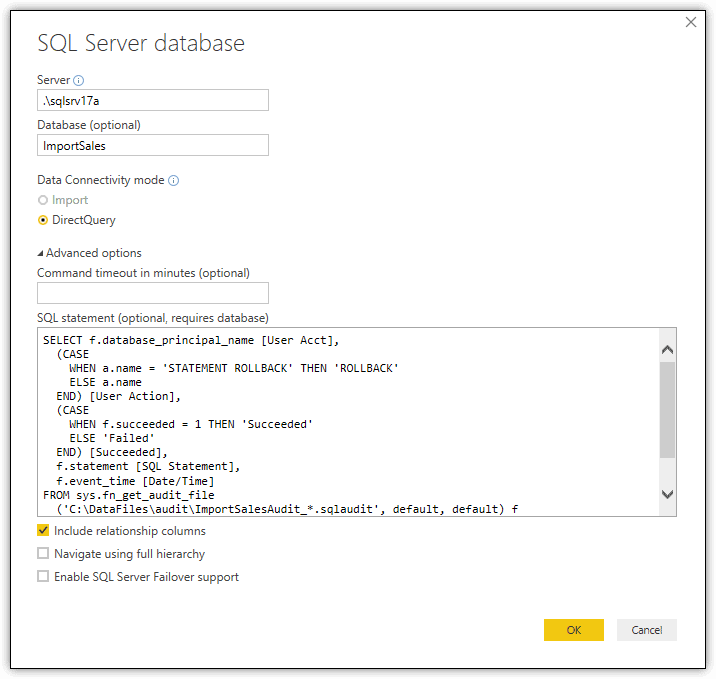
Figure 1. Defining a SQL Server connection in Power BI Desktop

To configure the connection:

  1. Type the SQL Server instance in the Server text box.
  2. Type the name of the database, ImportSales, in the Database text box.
  3. Select an option in the Data Connectivity mode section. I chose DirectQuery.
  4. Type or paste the SELECT statement into the SQL statement text box.

When you select DirectQuery, no data is imported or copied into Power BI Desktop. Instead, Power BI Desktop queries the underlying data source whenever you create or interact with a visualization, ensuring that you’re always viewing the most current data. Be aware, however, that if you plan to publish your report to the Power BI service, you’ll need to set up a gateway connection that enables the service to retrieve the source data. Also, note that you cannot create a Power BI Desktop report that includes both a DirectQuery SQL Server connection and an Import SQL Server connection. You must choose one or the other.

After you’ve configured the connection in the SQL Server database dialog box, click OK. This launches a preview window, where you can view a sample of the audit data, as shown in Figure 2.

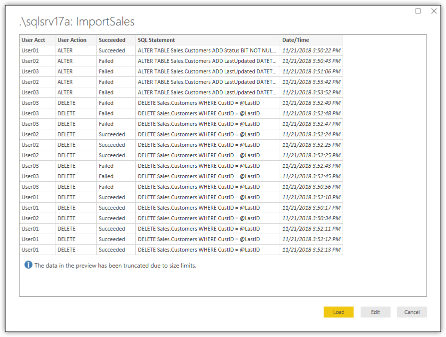
Figure 2. Verifying the SQL Server Audit data

If everything looks as you would expect, click Load to make the data available to Power BI Desktop, where you can use the data to add tables or visualizations. If you selected DirectQuery, you’re loading only the table schema into Power BI Desktop, with no source data imported until it is needed.

As noted earlier, you’re not limited to saving the audit data to log files. You can also save the data to the Application or Security log, but that means taking extra steps to get the data out of the logs and into a digestible format, such as a .csv file.

For example, you can export the data from Windows Event Viewer or the Log File Viewer in SQL Server Management Studio (SSMS), but the resulting format can be difficult to work with, and you could end up with much more data than you need. Another approach is to use PowerShell to retrieve the log data, creating a script that can be scheduled to run automatically. In this way, you have far more control over the output, although there’s still some work involved to get it right.

Regardless of how you make the data available to Power BI Desktop, the more important consideration is data security. The Security log might be the safest approach initially, but once you export the data to files, you’re up against the same issues you face when sending the data directly to log files. The data in those files needs to be fully protected at all times both at-rest and in-motion. There would be little point in implementing an audit strategy to comply with regulatory standards if the auditing process itself puts the data at risk.

Once you’ve made the test audit data available to Power BI Desktop, you can create reports that present the data in ways that offer different insights. Throughout the rest of the article, I show you several approaches that I’ve tried, using both tables and visualizations, in order to demonstrate ways you can present SQL Server Audit data. For details on how to actually create these components, refer to Part 7 of this series, Building Reports in Power BI Desktop.

Adding a Table to Your Report

One useful approach to presenting information is to make at least some of the data available in tables. For example, Figure 3 shows a table that includes all the audit data I pulled into Power BI Desktop. You can, of course, filter the data however you need to, such as with Slicers, depending on your specific audit strategy. The auditing that’s implemented for this article is very simple in comparison to the types and amounts of data that you will likely be generating.

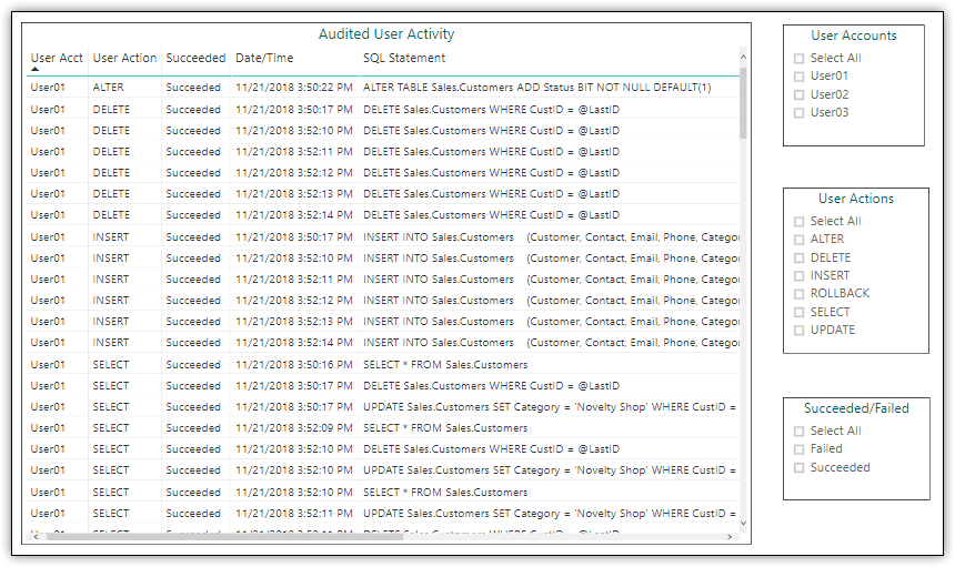
Figure 3. Adding a table and slicers to a report page

In addition to the table, I added three slicers to the report page for filtering the data by users, actions, and successes and failures. For example, Figure 4 shows the data I generated on my system after I filtered the information by the User03 account and the Failed status.

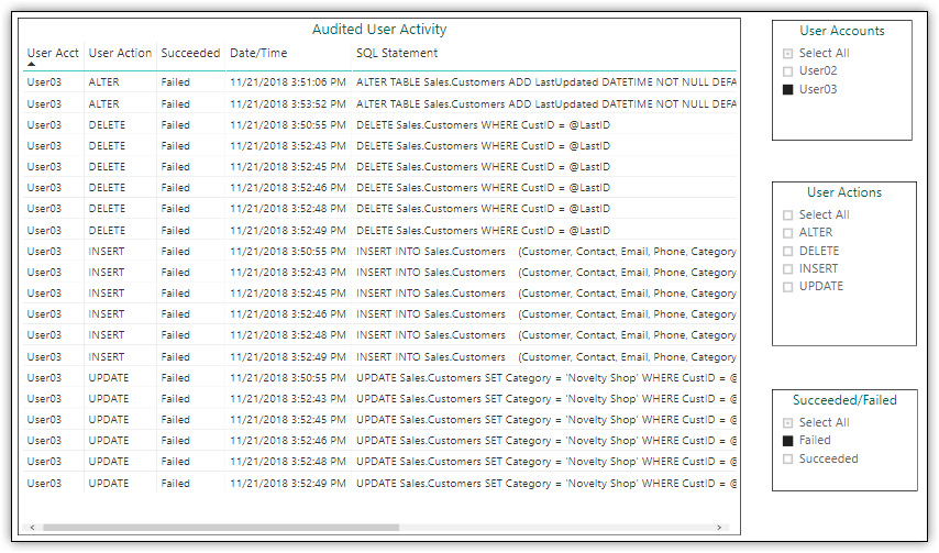
Figure 4. Using slicers to filter data in a table

When you apply a filter, Power BI updates the data in the table and slicers, based on the selected values. In this way, you have a quick and easy way to access various categories of data, without needing to manually weed through gobs of data or generate a new T-SQL statement each time you want to focus on different information.

Adding a Matrix to Your Report

Another effective way to provide quick insights into the data is to add a matrix that summarizes the data. For example, Figure 5 shows a matrix that displays the number of actions per user and action type. (A ROLLBACK statement is issued when a primary statement fails, such as when a user does not have the permissions necessary to run a statement.)

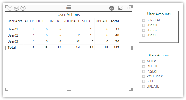
Figure 5. Adding a matrix and slicers to a report page

On the same report page as the matrix, I added two slicers, one for user accounts and the other for user actions, again allowing me to easily filter the data as needed.

What is especially useful about the matrix is that you can set it up to drill down into the data. In this case, the matrix allows you to drill to the number of actions that have succeeded or failed. For example, Figure 6 shows the matrix after drilling down into all users, although it’s also possible to drill down into specific users.

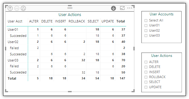
Figure 6. Drilling into a matrix

When setting up the drill-down categories in a matrix, you can choose the order in which to present each layer, depending on the type of data and its hierarchical nature. For example, this matrix can also be configured to drill down further into the T-SQL statements associated with each category.

Adding Visualizations to Your Report

Power BI Desktop supports a wide variety of visualizations, and you can import even more. You should use whichever visualizations help you and other users best understand the types of audit data you’re collecting. For example, Figure 7 shows a report page with three types of visualizations, each providing a different perspective into the audit data (keeping in mind that you’re working with a limited sample size).

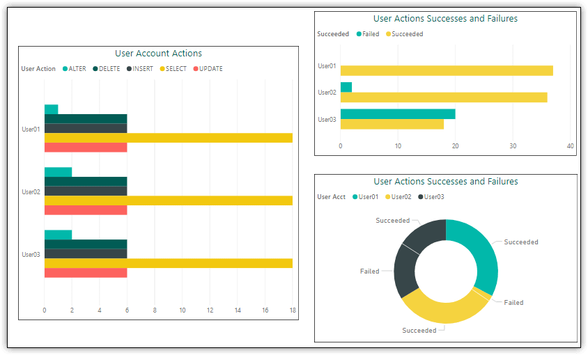
Figure 7. Adding visualizations to a report page

For all three visualizations, I filtered out the ROLLBACK actions, so the visualizations reflect only the statements that were initiated by the users, rather than those generated as a response to their actions. The visualizations on the left and top-right are clustered bar charts. The clustered bar chart lets you group related data in various ways to provide different perspectives.

For example, the clustered bar chart on the left groups the data by user, and for each user, provides a total for each action type. In this case, the DML actions show the same totals across all three user accounts because I ran the statements the same number of times. Even so, the visualization still demonstrates how you can use the clustered bar chart to provide a quick overview of the data from different perspectives, in this case, the types of statements each user has tried to run.

The clustered bar chart at the top right also groups the data by user, but then provides a total of statement successes and failures for each account, making it possible to see which users might be attempting to run statements that they’re not permitted to run.

The bottom right visualization is a basic donut chart. The visualization presents the same data as the clustered bar chart above it, but in a different way. If you hover over one of the elements, for example, you’ll get the percentage of total actions. What all this points to is that you can try out different visualizations against the same data to see which ones provide the best perspectives into the underlying information.

When you place elements on the same report page, Power BI automatically ties them together. In this way, if you select an element in one visualization, the other visualizations will reflect the selection. For example, if you click the Failed bar for User03 in the top right clustered bar chart, the corresponding data elements in the other visualizations will be selected, resulting in the nonrelated elements being grayed out.

Adding a Gauge to Your Report

Power BI Desktop also lets you add elements such as gauges, cards, and key performance indicators (KPIs) to a report. For example, I added the gauge shown in Figure 8 to display the number of ROLLBACK statements that were executed in response to the users’ failed attempts to run T-SQL statements.

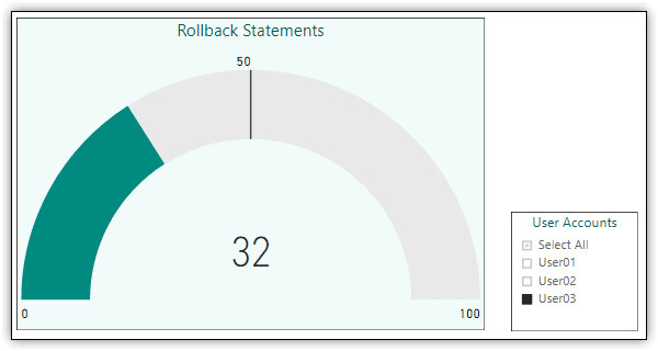
Figure 8. Adding a gauge to a report page

I also added a slicer for the user accounts to make it easy to see whether individual users are hitting the specified threshold. In Figure 8, the User03 account is selected in the slicer, so the gauge shows only the number of rollbacks that pertain to that user. The gauge also specifies a target of 50, but you can specify any target value.

The reason the target value is significant is that you can set alerts based on that value in the Power BI service (something you cannot do in Power BI Desktop). To use this feature, however, you must have a Power BI Pro license, which allows you to set up alerts that notify you regularly about potential issues. You can also set up alerts that generate email notifications on a regular basis. Plus, you can add alerts to card and KPI visuals.

Visualizing Audit Data in Power BI

Using Power BI to visualize SQL Server Audit data can provide you will a powerful tool for reviewing the logged information in a quick and efficient manner. What I’ve covered here only scratches the surface. There’s far more to SQL Server Audit and Power BI Desktop, and both topics deserve much more attention.

But this article should at least offer you a good starting point for understanding what it takes to use Power BI to work with SQL Server Audit data. It’s up to you to decide how far you want to take this and how extensively you might want to use the Power BI service, in addition to Power BI Desktop, keeping in mind the importance of protecting the audit data wherever it resides.

The post Power BI Introduction: Visualizing SQL Server Audit Data — Part 9 appeared first on Simple Talk.


from Simple Talk https://ift.tt/2r95L2o
via

There is a New COUNT in Town

We have all been using the COUNT(DISTINCT) function to return row counts for a distinct list of column values in a table for ages. With the introduction of SQL Server 2019, there is a new way to get an estimate of distinct row values and counts for a table. It is by using the new APPROX_COUNT_DISTINCT() function. This new function doesn’t return the actual number of rows for each distinct value in a table, but instead returns an approximate count for each distinct value. This new function uses fewer resources than the tried and true COUNT(DISTINCT) function. Let’s take a little closer look at this new function.

What Problem is APPROX_COUNT_DISTINCT() Trying to Solve?

The new APPROX_COUNT DISTINCT() function is trying to solve the “Count Distinct Problem.” More information about this problem can be found here. Basically, the problem is that counting distinct values requires more and more memory as the number of distinct values increases. At some point, SQL Server can no longer manage to maintain the count of distinct values in memory and must spill to tempdb. Spilling to tempdb causes overhead and leads to increased execution time.

The implementation of APPROX_COUNT_DISTINCT() has a much smaller memory requirement than the COUNT(DISTINCT) function. The algorithm used for this new function is HyperLogLog. This algorithm can estimate the number of distinct values of greater than 1,000,000,000, where the accuracy of the calculated approximate distinct count value is within 2% of the actual distinct count value. It can do this while using less than 1.5 KB of memory.

More Information About the APPROX_COUNT_DISTINCT Function

The APPROX_COUNT_DISTINCT function has been available in other vendor software packages for a while now, but it is new in SQL Server. It first became available in Azure SQL Database, and now has been released for on premises use with SQL Server 2019 Community Technical Preview (CTP) 2.0. This new function is design to quickly return the approximate number of unique non-null values in a group, when your data set has millions, or billions of rows, and many distinct values.

This APPROX_COUNT_DISTINCT() function is designed to give you the approximate aggregated counts more quickly than using the COUNT (DISTINCT) method. It does this by using the HyperLogLog algorithm, which reduces the memory footprint required to maintain a list of distinct values. Because less memory is needed, APPROX_COUNT(DISTINCT) is, therefore, less likely to spill to tempdb when aggregating millions or billions of rows of data. This equates to shorter execution times compared to using the COUNT(DISTINCT) method.

The documentation states that this new function “guarantees up to a 2% error rate within a 97% accuracy.” Therefore, if speed is more important than absolute accuracy of the distinct count, then you might want to consider using this new function.

Invoking this function is similar to using the COUNT(DISTINCT) function. Here is the syntax:

APPROX_COUNT_DISTINCT ( expression )

The expression can be any type, except for image, sql_variant, ntext, or text value.

Testing APPROX_COUNT_DISTINCT() for Performance

In order to test out the performance of this new function, I’ll use a specific use case to determine out how fast APPROX_COUNT_DISTINCT() runs as compared to COUNT(DISTINCT. In addition to verifying the speed, I’ll also look to see if I can detect if this new function uses a smaller memory footprint than the old COUNT(DISTINCT) standby.

To gather and compare these metrics, I’m going to use this specific hypothetical use case and situation:

Use Case:

Develop a dashboard indicator that shows whether the number of unique IP addresses that have accessed our site for the current month is more, less or the same as the prior month.

Situation:

I work at an internet search engine, and I am responsible for building queries to run against some of the data we have collected. One of the things we track are the IP addresses for every visit to our site. We collect billions of rows of data every month. My boss has asked me to develop a query that can be used as a dashboard trend indicator that will show whether the number of unique IP Addresses coming to our site has gone up (+) or down (-) in the current month, as compared to the prior month. My boss requires this new query to run as fast as possible across our IP Address tracking table that contains billions, and billions of rows. My boss is willing to accept some level of lesser precision in the accuracy of the number, provide the indicator and percentage of change can be produced more quickly than a method that has absolute accuracy.

To create a testing environment, I created a database and populated a table named Visits2 that has a billion rows of randomly generated data. You can find the code I used to create my sample database in Listing 3, at the end of this article.

First, I want to test how fast the APPROX_COUNT_DISTINCT() function runs as compared to the COUNT(DISTINCT) function. For this test, I ran two SELECT queries that supported my use case. The first SELECT statement uses the COUNT(DISTINCT)function, and the second SELECT statement uses the APPROX_COUNT_DISTINCT() function. This code, found in Listing 1, generates a count of the number of unique IP Address that have accessed our site for July and August. You can also turn on “live query statistics” if you wish to monitor the progress of each SELECT statement while they are running.

SET STATISTICS TIME ON;
GO
SELECT COUNT(DISTINCT IP_Address) AS NumOfIP_Addresses, DATEPART (month,VisitDate) AS MonthNum 
FROM [dbo].[Visits2] 
WHERE DATEPART (month,VisitDate) IN (7, 8)
GROUP BY DATEPART (month,VisitDate);
GO
SELECT APPROX_COUNT_DISTINCT(IP_Address) AS NumOfIP_Addresses, DATEPART (month,VisitDate) AS MonthNum 
FROM [dbo].[Visits2] 
WHERE DATEPART (month,VisitDate) IN (7, 8) 
GROUP BY DATEPART (month,VisitDate);

Listing 1: Code to compare COUNT(DISTINCT) and APPROX_COUNT_DISTINCT() functions

This code turns on time statistics and runs each SELECT statement. I will use the time statistics produced by running this code to determine how much CPU and elapsed time it takes to get distinct IP address counts for July and August. In Results 1, you can see the CPU and elapsed times I got when I ran the code in Listing 1.

Results 1: The timing results when running the code in Listing 1

In Results 1, I show the timing results of the output produced by setting the STATISTICS TIME ON, for the two SELECT statements. The first set of times are from the COUNT(DISTINCT) query, whereas the second set of times are from the APPROX_COUNT_DISTINCT query. As you can see, APPROX_COUNT_DISTINCT used less CPU and elapsed time compared to the COUNT(DISTINCT)query. The APPROX_COUNT_DISTINCT() function ran a little over 6% faster than the COUNT(DISTINCT) function and uses almost 24% less CPU.

To determine the number of memory grants used by each SELECT statement, I used the output of the execution plan. In Results 2 you can see the execution plan from these two SELECT queries.

Results 2: Execution Plan code in Listing 1

The first thing you might notice when comparing these two executions is that the Cost of the Hash Match operation for the COUNT(DISTINCT) function takes more than twice as long to run as the Hash Match operation for the APPROX_COUNT_DISTINCT() function.

When I hover over the Hash Match operator for the COUNT(DISTINCT) function, I can see it spilled to disk (see Results 3), but when I hover over the Hash Match operator for the APPROX_COUNT_DISTINCT function, it did not spill to disk (see Results 4).

Results 3: Details of Hash Match operation for COUNT(DISTINCT) function

Results 4: Details of Hash Match operation for APPROX_COUNT_DISTINCT function

To display the number of memory grants between the two different functions, I hover over the SELECT icon in the execution plan. When I hover over the COUNT(DISTINCT) SELECT icon I get the results in Results 5, and when I hover over the APPROX_COUNT_DISTINCT SELECT icon I get the results in Result 6.

Results 5: Memory Grants for COUNT(DISTINCT)

Results 6: Memory Grants for APPROX_COUNT_DISTINCT()

As you can see, the COUNT(DISTINCT) function required 1,847,736 memory grants, whereas the APPROX_COUNT_DISTINCT() function only required 24,776 memory grants. This means the COUNT(DISTINCT) took 74 times as many memory grants over the new APPROX_COUNT_DISTINCT() function. Based on this, you can see the APPROX_COUNT_DISTINCT() function had a significantly smaller number of additional memory grants required versus the COUNT(DISTINCT) function.

Testing APPROX_COUNT_DISTINCT() for Accuracy

In addition to performance testing, I also wanted to test the accuracy/precision of distinct values produced between the COUNT(DISTINCT) and the APPROX_COUNT_DISTINCT() functions. To determine the precision difference between the two functions, I compared the number of distinct values produced by the two different SELECT statements in Listing 1. The COUNT(DISTINCT) function returned a count of 16,581,375 distinct IP address for July, whereas the APPROX_COUNT_DISTINCT() function returns a count of 17,075,480 for July. By comparing these two numbers, I can see that the APPROX_COUNT_DISTINCT() function is off by a little over 2.97%. Since this number was not within 2% error rate as documented, I contact Microsoft about this.

An engineer at Microsoft told me that the SQL Server engine uses a “sophisticated analytic sampling method” to produce an estimated count, and because of this, it is possible to build a contrived table that throws off the sampling method and produces dramatically inaccurate results.

From this first test, I can see that the APPROX_COUNT_DISTINCT() function does, in fact, run faster and requires fewer resources over the COUNT(DISTINCT) function. The only problem I ran across with this first test, was that I had more than a 2% precision error when generating the approximate count, over the real distinct count value. In my case, I found the precision error was 2.97%, which according to documentation can occur.

Since my initial testing found the APPROX_COUNT_DISTINCT() function returned a distinct count that was more than 2% different than the actual distinct count, I decided to run some additional precision testing. The additional SELECT statements I will be testing can be found in Listing 2.

SELECT COUNT(DISTINCT ID)           AS COUNT_ID,
           COUNT(DISTINCT I100)      AS COUNT_I100,      
           COUNT(DISTINCT I1000)     AS COUNT_I1000,      
           COUNT(DISTINCT I10000)    AS COUNT_I10000,    
           COUNT(DISTINCT I1000000)  AS COUNT_I1000000,  
           COUNT(DISTINCT I10000000) AS COUNT_I10000000  
FROM Visits2;
GO
SELECT APPROX_COUNT_DISTINCT(ID)           AS COUNT_ID,
           APPROX_COUNT_DISTINCT(I100)      AS COUNT_I100,      
           APPROX_COUNT_DISTINCT(I1000)     AS COUNT_I1000,      
           APPROX_COUNT_DISTINCT(I10000)    AS COUNT_I10000,    
           APPROX_COUNT_DISTINCT(I1000000)  AS COUNT_I1000000,  
           APPROX_COUNT_DISTINCT(I10000000) AS COUNT_I10000000  
FROM Visits2;

Listing 2: Additional Testing Queries

The code in Listing 2 will identity the number of unique counts for columns that have a different number of unique values. I will use this code in Listing 2 to determine the number of different values it takes for the APPROX_COUNT_DISTINCT function to produce a count which is different than the actual number of unique values produced by the COUNT(DISTINCT) function. The code from Listing 2 produces the output found in Results 7.

Results 7: Results from running code in Listing 2

As you can see by looking at Results 7, the APPROX_COUNT_DISTINCT() function produces the same number as compared to the COUNT(DISTINCT) function when the number of unique values is low. In my case less than 1,000 unique values. But for each column that had more than 100 values, the APPROX_COUNT_DISTINCT() function produced an approximate number was more or less than the actual number generated by the COUNT(DISTINCT) function. This test shows that when the actual number of distinct values in a table increases, the APPROX_COUNT_DISTINCT() functions don’t produce the same number of distinct values as the COUNT() function, however, it is close. Therefore, if your table contains a large number of distinct values, then expect this new function to produce a count value that is somewhat different than the actual number of distinct values.

Conclusions Based on My Initial Testing

From the few simple tests I ran here against my generated sample data, I have made the following observations:

  • The APPROX_COUNT_DISTINCT() function does return a distinct count number faster than the COUNT(DISTINCT) function.
  • The COUNT(DISTINCT) function requires more memory grants than the APPROX_COUNT_DISTINCT() function.
  • In one situation, I able to returns a unique count value that had more than a 2% error rate.
  • If the number of distinct values for a given column is low, then the APPROX_COUNT_DISTINCT() function returns the same count value as the COUNT(DISTINCT) function.

Should you start using the APPROX_COUNT_DISTINCT()function? That’s a good question. I suppose it depends on your situation. I was pleasantly surprised at how much I was able to improve the runtime and reduce the memory footprint using the APPROX_COUNT_DISTINCT() function over the COUNT(DISTINCT) function. But I was little concerned how easy it was for me to retrieve an aggregated count value that had a precision error of more than 2%. My Visits2 table was very contrived but did expose the improvement and drawbacks of using the APPROX_COUNT_DISTINCT() function. Therefore, before using this new function in a production environment, I would suggest developing a more exhaustive set of tests against real data to verify that any precision errors are within an acceptable range for each situation. As with any new feature, I suggest you identify what the new feature does and then test the heck out of it to verify it provides the improvements you desire in your environment.

Code Used to Create Sample Test Data

In Listing 3, you will find the code I used to create my contrived sample database (SampleData) and the table (Visits2) I used to support my testing. Keep in mind that the code in this listing is not very efficient at creating my sample data. It took over an hour on my laptop to create the billion-row table I used for testing.

-- Create Sample DB with SIMPLE recovery
CREATE DATABASE SampleData
 CONTAINMENT = NONE
 ON  PRIMARY 
( NAME = N'SampleData', FILENAME = N'D:\SQL Server 2019\SampleData.mdf' , SIZE = 65GB, FILEGROWTH = 5GB)
 LOG ON 
( NAME = N'SampleData_log', FILENAME = N'D:\SQL Server 2019\SampleData_log.ldf' , SIZE = 5GB, FILEGROWTH = 5GB);
GO
ALTER DATABASE SampleData SET RECOVERY SIMPLE;
GO
-- Set database context
USE SampleData;
GO
-- Create table to hold sample data
CREATE TABLE Visits2
(
        ID         INT, 
        I100       INT, 
        I1000      INT, 
        I10000     INT, 
        I100000    INT,
        I1000000   INT, 
        I10000000  INT,
        IP_Address VARCHAR(15),
        VisitDate  DATE
);
GO
-- Create Tally Table
GO
CREATE VIEW vw_Tally AS 
        --Itzik style tally table
        WITH lv0 AS (SELECT 0 g UNION ALL SELECT 0)
                ,lv1 AS (SELECT 0 g FROM lv0 a CROSS JOIN lv0 b) -- 4
                ,lv2 AS (SELECT 0 g FROM lv1 a CROSS JOIN lv1 b) -- 16
                ,lv3 AS (SELECT 0 g FROM lv2 a CROSS JOIN lv2 b) -- 256
                ,lv4 AS (SELECT 0 g FROM lv3 a CROSS JOIN lv3 b) -- 65,536
                ,lv5 AS (SELECT 0 g FROM lv4 a CROSS JOIN lv4 b) -- 4,294,967,296
                ,Tally (n) AS (SELECT ROW_NUMBER() OVER (ORDER BY (SELECT NULL)) FROM lv5)
        SELECT TOP (1000000) n
        FROM Tally
        ORDER BY n;
        
GO      
-- Populate Visits2 with sample data
SET NOCOUNT ON;
DECLARE @Max bigint = (select ISNULL(max(ID),0) From Visits2);
WHILE @Max < 1000000000 BEGIN 
        
        WITH TallyTable AS (
                
                SELECT n + @Max as N, 
                        CAST(RAND(CHECKSUM(NEWID())) * 255 as INT) + 1 AS A4,
                        CAST(RAND(CHECKSUM(NEWID())) * 255 as INT) + 1 AS A3,
                        CAST(RAND(CHECKSUM(NEWID())) * 255 as INT) + 1 AS A2, 
                        1.0 + floor(1 * RAND(convert(varbinary, newid()))) AS A1,
                        DATEADD(DD, 1.0 + floor(62 * RAND(convert(varbinary, newid()))),'2018-07-01') AS VisitDate
                FROM vw_Tally)
        INSERT INTO Visits2 (ID, I100, I1000, I10000,   I100000,        I1000000, I10000000, IP_Address, VisitDate)
        SELECT                          n,      n%100, n%1000, n%10000, n%100000,       n%1000000, n%10000000, 
                                CAST(A1 AS VARCHAR) + '.' + CAST(A2 AS VARCHAR) + 
                 '.' +  CAST(A3 AS VARCHAR) + 
                 '.' +  CAST(A4 AS VARCHAR), VisitDate
        FROM TallyTable 
        set @Max = (select ISNULL(max(ID),0) From Visits2);
END
-- CREATE UNIQUE CLUSTERED INDEX
CREATE CLUSTERED INDEX IX_SampleData_Visits2_ID ON dbo.Visits2(ID);   
GO

Listing 3: Script to create database and Visit2 table

The post There is a New COUNT in Town appeared first on Simple Talk.


from Simple Talk https://ift.tt/2DQGGkm
via

Treating SQL Server as an Object with PowerShell

In my previous article, I showed you how to use PowerShell to create a script to dump out all the tables of your databases to files. One concept that was introduced at the time was that PowerShell treats everything as an object. In this article, you’ll get a chance to take a closer look at this.

Open the PowerShell ISE and execute the following commands

dir C:\

The results are about what you’d expect. Your output, of course, will vary a bit. The format is a little different from what you’d see in the CMD processor (it’s closer to a Unix style directory listing), but it’s recognizable as a directory listing.

Now try:

#this assumes you have a default instance on your local system, if you don't, change the word default to the name of your instance or change the server name
$sqlserver = 'localhost\default'
invoke-sqlcmd
cd sqlserver:\sql\$sqlserver
dir databases

Now you’ll get back something very different from a filesystem listing, but it should be something that should be somewhat recognizable, a list of databases.

Back up a step and discover what else you can see. Enter the following command:

get-psdrive

This output shows all the current locations that PowerShell can treat as a drive tree. Since this was run on a server as administrator, I could drill down and look at the Active Directory information. You probably will not see this on your machine. You will also see other objects that are specific to your machine. You can’t usually see SQLServer, but using the Invoke-SQLCmd forces the loading of the code necessary to make that happen. To access any of these objects, just type cd <objectname>.

I used the cmdlet Invoke-SQLCmd earlier in the article. What that did, however, was merely to force the loading of a PowerShell library. You can load the library directly with the following command when it’s not already loaded.

import-module sqlps

You may get a warning message, about some verbs being unapproved. This warning doesn’t impact your ability to use them. You can ignore the warning message. If you’re curious about what cmdlets are being imported, try viewing both approved and unapproved by running the following command.

import-module sqlps -verbose

If, for some reason, you want to remove all the SQL related cmdlets, use

Remove-Module sqlps

I can’t think of a reason to do that, other than perhaps to free up memory.

PowerShell treats the objects in SQL Server like it treats files in a directory. By running dir databases, you get a list of your user databases. The system databases are not listed, but, you can treat them like hidden files and use the –force parameter.

ls databases -force

I changed commands slightly here and used ls instead of dir. Dir is an alias for ls, which in turn is an alias for get-childitem. PowerShell uses a lot of aliases that map to cmdlets of the verb-noun form. Since it’s shorter and the syntax is closer to the Unix form, I will use ls from now on.

Just like in a Windows or Unix filesystem, you can navigate further. Run this to see the objects listed under the SQLServer directory.

ls .

You should recognize these as objects and collections of objects that are found on SQL Server, for example, LinkedServers and Logins. You can explore any of those areas. To see the logins that exist on this server, run:

ls logins -force

Notice that I used the –force parameter. Without that, some of the above logins, like sa, would not show up.

Looking at Objects

So far, the examples explore SQL Server like a filesystem. But again, PowerShell is about the objects.

$logins = ls logins -force
$logins

This will show you all the logins in the system after the collection has been saved in a variable. This command is useful, but what if you want just a list of the sqllogins?

ls logins -force | where {$_.logintype –eq 'sqllogin'}

This takes the results of the ls logins command and pipes it to the where command. You have to tell where what to act on. $_ is a shorthand for referencing the most recently used object; in this case the output of the ls logins –force command. PowerShell uses -eq (and –gt and -lt and –ne) to test for equality. This command will show you all logins on the server that are of the type sqllogin. It does this by looking at the logins property of logintype.

This can also be done by using two commands, saving the collection in a variable first so that it can be reused:

$logins = ls logins -force
$logins | where {$_.logintype –eq 'sqllogin'}

Every object has properties, some more than others. To see what properties and methods an object may have, pipe it to the get-member cmdlet.

$logins | get-member | out-gridview

Or if you want to be very frugal in your typing, you can use aliases:

$logins | gm | ogv

By piping the output to out-gridview, you can take advantage of the GUI and have an easy to read window that allows you to filter further.

And with a filter applied:

This is showing you all the login properties related to passwords.

Viewing Properties in Multiple Servers

Imagine the auditor has come to you and wants to know which logins exist on the SQL Server instance, which ones are enabled, and which ones have password expiration enabled. You could do this as a T-SQL query, but you need to execute this against 100 different servers.

Start with:

$logins | select-object name,ispasswordexpired, MustChangePassword, isdisabled, passwordexpirationenabled

You most likely will get results like this:

The select-object command permits selecting which properties you want from the logins object. However, you may want it in a more readable format. This is where the format-table cmdlet that was mentioned in the last article can be useful.

ls logins -force| select-object name,ispasswordexpired, MustChangePassword, isdisabled, passwordexpirationenabled | format-table

You now have the results for one server, but you have 99 more to go. You can take advantage of the looping from the last article and the fact that you can use an array of strings:

#Update the array to reflect your instances
$sqlservers = @('SQL01\default','SQLDB_02\sqlexpress','SalesSQL\default', 'SalesSQL\TEST_Instance')
foreach ($sqlserver in $sqlservers) 
{
cd sqlserver:\sql\$sqlserver
ls logins -force| select-object name,ispasswordexpired, MustChangePassword, isdisabled, passwordexpirationenabled | format-table
}

Note that the array contains the name of the SQL Server and the instance on that server. That makes it easier to handle the servername and instances on that server. This code will loop through and display the name of the instance and the logins on it:

The auditor is happier, but this is still not the most useful format. You can take it one step further by updating your script a tad:

#Update the array to reflect your instances
#Update the output path if necessary
$sqlservers = @('SQL01\default','SQLDB_02\sqlexpress','SalesSQL\default', 'SalesSQL\TEST_Instance')
$Filepath =  'C:\Users\administrator.YOURDOMAIN'
foreach ($sqlserver in $sqlservers) 
{
    cd sqlserver:\sql\$sqlserver
    write-host $sqlserver
    write-host "===================="
    ls logins -force| select-object name,ispasswordexpired, MustChangePassword, isdisabled, passwordexpirationenabled | format-table
    $logins = ls logins -force| select-object name,ispasswordexpired, MustChangePassword, isdisabled, passwordexpirationenabled 
    
     $logins | ConvertTo-Json | out-file -FilePath "$Filepath\$($sqlserver -replace '\\','_').json"
    $logins | ConvertTo-Csv | out-file -FilePath "$Filepath\$($sqlserver -replace '\\','_').csv" 
}

The results are saved into a new object: $logins. Since you’re not sure if your auditor will want the results in a CSV file (which they can easily open in Excel, which it seems every auditor loves) or perhaps they want to be able to suck it into another program using JSON, you’ve nicely provided them with a choice of either. One of the things you’ll notice is that the script replaces the backslash (\) in the server name with an underscore (_). This is to prevent the OS from interpreting it as a subdirectory which would possibly give an error when writing to disk.

Speaking of errors, when you run the above script, you may get multiple warnings with the format:

WARNING: Could not obtain SQL Server Service information. An attempt to connect to WMI on ‘ SQL01’ failed with the following error: SQL Server WMI provider is not available on gage. –> Invalid namespace

This error appears to occur if the WMI agent is set up as a local login and not a domain login. You can suppress this using -WarningAction SilentlyContinue in the appropriate places, in this case after the –force and at the end of the select-object. Of course, suppress warnings at your own risk.

However, that only handles warnings. If you have errors, you could also silently continue, but that’s probably ill-advised. You should add in a little basic error handling. The most common error is that the server you’re trying to reach isn’t available when you run the scripts. It may be off-line, being rebooted or something else has happened. To solve that, you need to trap the error and handle it.

PowerShell, like most modern languages, supports try-catch-finally. There’s an important detail, however, to understand with error handling. Try-Catch only catches errors if you tell it to. Otherwise, the script continues to run. In other words, you will need to tell the CmdLet to STOP on an error. The default is to continue. In the example below, assume that FOO\BAR is currently offline. After attempting to connect to FOO\BAR, it will leave an error message in a file along with the CSV and JSON files.

#Update the array to reflect your instances
#Update the output path if necessary
$sqlservers = @('SQL01\default','SQLDB_02\sqlexpress','SalesSQL\default', 'SalesSQL\TEST_Instance', 'FOO\BAR')
$Filepath = 'C:\Users\administrator.YOURDOMAIN'
foreach ($sqlserver in $sqlservers) 
{
 
    write-host $sqlserver
    write-host "===================="
    try
    {
        cd sqlserver:\sql\$sqlserver -ErrorAction stop -WarningAction SilentlyContinue 
        ls logins -force -WarningAction SilentlyContinue | select-object name,ispasswordexpired, MustChangePassword, isdisabled, passwordexpirationenabled  | format-table 
        $logins = ls logins -force| select-object name,ispasswordexpired, MustChangePassword, isdisabled, passwordexpirationenabled # | format-table
     $logins | ConvertTo-Json | out-file -FilePath "$Filepath\$($sqlserver -replace '\\','_').json"
    $logins | ConvertTo-Csv | out-file -FilePath "$Filepath\$($sqlserver -replace '\\','_').csv" 
    }
    catch
    {
        $ErrorMessage = $_.Exception.Message
        "Error:Could not retrieve logins: $ErrorMessage." | ConvertTo-Json | out-file -FilePath "$Filepath\$($sqlserver -replace '\\','_').json"
        "Error:Could not retrieve logins: $ErrorMessage." |  out-file -FilePath "$Filepath\$($sqlserver -replace '\\','_').txt"
    }
}

Notice that this is only catching errors if the CD CmdLet to switch instances fails. If any of the other CmdLets fails, the script will continue without being detected.

You now have a quick script that will give your mythical auditor the data they want on logins, broken down by instance. If there is an instance that isn’t responding, you’ll know about that as well. That means you can get out of the office without having to work overtime.

This sort of script could also be made a part of a scheduled task that could email you the results on a monthly (or more often) basis.

Updating Properties

But imagine that the auditor wants you to rename and then disable the sa account. This is a situation that came up with one of my clients. Again, you could go into each server manually, but this could take forever. Instead, take what you have learned and automate it using PowerShell.

Please note: The scrips above merely looked at your current server(s). The scripts below will make modifications to your server(s) and should only be run in a test environment until you’re comfortable running them.

Your first inclination may be to look for a cmdlet that can change login properties. To see what cmdlets are available within the sqlps module, you can invoke:

get-command -module sqlps

Unfortunately, nothing here looks all that useful. You could use Invoke-SqlCMD, but that ignores the object focus of this article. But there is a better way. Instead of looking for types of logins as you did above, you are going to look for a specific login, in this case, the sa login.

Since you may have ended up on the wrong server from the loops above, make sure to get back to the server you want to work on before saving the logins.

$sqlserver = 'localhost\default'
cd sqlserver:\sql\$sqlserver
$login = ls logins -force | where {$_.name -eq 'sa'}

Now you have an object, $login that contains the particulars of the sa login. If you recall from when you ran $logins | gm | ogv, there were a number of methods that were displayed. A quick search of $login | gm | ogv is quite useful. Once the GUI is displayed, enter disable as the filter.

You can make use of that and the closely related property IsDisabled and run the following lines:

$login.IsDisabled
$login.disable()
$login.IsDisabled

If the account was originally enabled, you’d see that the sa login has changed from being enabled to disabled. If you want to enable it again, you would simply run

$login.Enable()

But remember, your overanxious auditor also wants you to rename the login. Again, using the method associated with the login, you can do that simply as:

$login.Rename('foo_sa')
$login

And you’ll see your results show that the login is now named foo_sa. You can wrap the scripts to disable and rename your sa account into the code above to run it against multiple servers.

The primary focus of this article is using sqlps to access logins, but, as you will recall from one of the first scripts, ls ., you have access to almost any part of your SQL Server that you want. For example, you could get a list of all your databases with some essential information.

When I’m working in a new environment, I like to know what the recovery model of the databases are and what collations they are, and possibly more information.

Again, a simple ls unlocks this information:

$databases = ls .\databases
$databases | Select-Object name, recoverymodel, collation, owner | format-table

To see all the various properties you can access, execute:

$databases | gm | ogv

You can get an amazing amount of information from running ls against your databases. For example, you can see all the stored procedures in a database, or synonyms and more. In addition to properties, you also have access to the various methods associated with the object.

If you run the following code, you will get different results for each resulting object.

cd .\databases 
$databases = ls . -Force #since we want the system databases also 
$singledb = ls master
$databases | gm | ogv
$singledb| gm | ogv

The first is an object containing multiple databases; the second is an object that contains the sub-objects of master (think of them like subdirectories of a directory). It’s not actually a single database object. For that, you need to do what you did with logins above and filter $databases for a specific database.

$onedatabase = $databases |where { $_.name -eq 'master'}
$onedatabase | gm | ogv

If you want to see the different types of each object ($databases, $singledb, $onedatabase) execute the following, each separately. Otherwise it appears that PowerShell will show the results in an order of its choosing.

$databases.GetType()
$singledb.GetType()
$onedatabase.GetType()

Now you can perform actual operations on the database. For example, if you had a database that was set to autoclose and you wanted to make sure that none of the databases were set that way, you could write a quick script to go through your server and disable autoclose on all your databases

For the following script, make sure you have run the cd .\databases command. You will also need to make sure that the AutoClose setting is set on a database before connecting. The prompt should look similar to PS SQL SERVER:\SQL\localhost\default\databases. If not, change directories before running the code.

$databases = ls .
$autoclosed = $databases | where {$_.autoclose -eq 1} 
foreach ($db in $autoclosed) 
{
    $db.name
    $db.autoclose = 0
    $db.alter()
}

You could wrap the above script in one of the scripts that loops through your servers, and you’d be able to execute this across all your servers if you wanted to. This means in a half-dozen or so lines; you can make updates across 1, 2, or 1000 servers in your organization with minimal effort. Of course, to quote Spiderman’s Uncle Ben, with great power comes great responsibility! So be careful of your newfound power.

Conclusion

Hopefully, this post has helped you to understand the power of treating SQL Server in an object-oriented fashion, and you can begin to use its features to manage across all the servers in your organization.

The post Treating SQL Server as an Object with PowerShell appeared first on Simple Talk.


from Simple Talk https://ift.tt/2zxaO13
via

New Technologies to Study

One great result from PASS Summit, especially when we are close to a new SQL Server release, is to identify important technologies to study on the following year.

PASS Summit 2018 was great, with sessions about many new technologies giving us very good guidance on where to focus our study for the new year. Let’s talk about some of these new technologies.

Of course, everything here is my current knowledge and information from the event about these new technologies, let’s talk about them on the comments.

Hyperscale


The 2nd day Keynote on PASS is well known for being a mind-blowing keynote and this year was no different.

You can watch the keynote here

However, the real mind-blowing part starts on 41:36, when the speaker invited to the stage starts explaining how Microsoft created a system of infinity, yes, infinity scalability, going deep in detail about the architecture of the Hyperscale system.

This is, for sure, something to be studied and tested if possible.

By the way, you can find more free videos from PASS Summit 2018 here

Intelligent Query Processing


First and foremost, why change the name? We are barely getting used to adaptive query processing!

PASS Summit Intelligent Query Processing

The idea of the adaptive query processing is to adapt the plan during the execution. On the other hand, the new features being included are more intelligent behaviour, don’t fit under the adaptive query processing scope. Being so, we have a new name, Intelligent Query Processing, which includes Adaptive Query Processing and other new features more.

Name explained, but what about row vs batch mode, the most expected new feature?

Well, among the three kinds of adaptive query processing, only memory grant feedback will be working with row mode, all the other remain the same.

However, there is a catch: some expensive analytic queries will be changed to batch mode even without a Columnstore Index, thus they will be able to use all batch mode features.

You can check more details about Intelligent Query Processing and also find some demo scripts on this link  

Big Data Cluster


Big Data Clusters is, in summary, the SQLServer version of a Hadoop cluster, using HDFS to store data.

PASS Summit Big Data Cluster

SQL Server core was redesigned as microservices and each node of a big data cluster uses Kubernetes to be executed. I’m not sure yet what kind of impact this will have on the DBA – will we need to learn about Kubernetes?

The Big Data Cluster is comparable to the PWD, but PWD is made for relational data, while the BDC uses HDFS, so it’s made for unstructured data. SQL Data Warehouse is the cloud version of PWD, it’s also made for relational data.

The best comparison is with Azure Data Lake. On one hand, Big Data Cluster is the technology to enable us to build an on-premise data lake. On the other hand, the architecture is completely different, Azure Data Lake uses U-SQL while the big data clusters will use T-SQL

So, how will all these technologies fit together? For now, no one has no idea, but my crystal ball believe these solutions will be integrated somehow in such a way they all can be managed from azure data studio

You can check more about big data clusters here 

Query Performance and Tunning Improvements


Pedro Lopes and Joseph Sack did a great work introducing a lot of new features that are already in preview. Let’s do a small summary about them.

SSMS 18 includes a new graphic for Wait Stats categories. The capture of the wait stats in SQL Server 2017 was already great and now we have a new graph to show the values for us.

A lot of new information was in the execution plan:

  • Active trace flags
  • Statistics used during the compilation, including the modification count
  • UDF CPU and elapsed time
  • Grant and used memory per thread
  • A lot more warning details

This will be very useful when analyzing the performance of a server. Have you read my articles about querying the plan cache (here and here)? Using all these new information we can build very interesting queries to check about many problems on the existing query plans that we couldn’t check before – and we can also query them inside query store system tables, not only on the plan cache.

You can read more about SSMS new features here 

Table Variables Deferred Compilation is also a very good improvement. If we can’t convince them to use temp tables, let’s improve the table variables.

A query against a temp table already uses deferred compilation, meaning that the query will only be compiled on the first execution of the query, not together with the entire batch, so the batch will be called, create the table, fill it and only then the query against the temp table will be compiled.

On the other hand, a usual query against a temp variable is compiled together the entire batch, when the variable is not filled yet, so the query is compiled considering a total of 1 record.

The change is simple: Now queries against table variables also use deferred compilation, waiting for the execution of the statement to be compiled and improving query performance.

More details about this new feature on this link 

On the entire session, however, one of the features that most impressed me was the Lightweight Query Execution Statistics Profile. The final result is simple: using SSMS 18 we can view the execution plan of an existing online session in SQL Server without the complex infrastructure that was required before.

This feature is also available from SQL Server 2016 SP 1: you only need to enable TF 4212

Power BI New Features


Power BI usually has so many new features that It’s very easy to get lost among them. Two new features caught my attention:

Support for Reporting Services files: Power BI supports the publishing of reporting services files. This is a great feature for migration of environments from reporting services to power bi, enabling the users to continue using the old reports and migrate than easily to a new format. You can check more about this on this link

Dataflows: The Dataflows are an evolution of the power query, although not exactly a replacement. The Power Query code is stored within the Power BI file, so if you need to use the same data source again, you may need to copy the M script to a new PBIX file.

The Dataflow, on the other hand, is stored and processed on power bi online. It imports the data to Azure Data Lake storage on Azure using a text format to store the data. You can re-use the data from the ADL storage and schedule the update online on the Power BI service. The process is closer to an ETL process, being able to use ADL storage either for intermediate steps for the transformations and for the final data.

As usual, new features created by Microsoft raise many questions. How will this fit together with other technologies, such as ADFv2 which enable us to execute SSIS packages on the cloud? Is Microsoft going too far on self-service BI and enabling users to create small monsters or will be this, in the end, easier to manage than the alternatives?

Matt Allington published an interesting article and video about Dataflows, you can check on this link

Azure SQL Database Managed Instances


PASS Summit Managed Instances

The Managed Instances got many sessions during PASS Summit. Before this new Azure service, we need to choose: We could use PAAS with SQL Databases on database level, but if we need any instance level service we would need to use IAAS, creating our own virtual machines.

Using the new Managed Instances we can have instance level services such as SQL Server Agent, replication, SQL Audit and many more on a PAAS environment, avoiding the need to manage an entire virtual machine such as in IAAS environments.

One of the most impressive features of the Manage Instances services is the Always on Availability Groups as a PAAS service.

You can check more details about managed instances here 


Conclusion

We have, for sure, a lot to study on the following year, until next PASS Summit comes to increase this list even more. You can start checking these links:

Preview SQL Server 2019 now

Join the early adoption program

See what’s new in SQL Server 2019

The post New Technologies to Study appeared first on Simple Talk.


from Simple Talk https://ift.tt/2RkVueV
via

Wednesday, November 28, 2018

Common Sense Data Science

Data science is so hip today that everyone is doing it. Everyone is showing off their ‘data science muscles’ by how much data they can lift and in what amazing ways the lifting is done. However, only some are showing that they can work in a smart way, and even fewer are showing common sense.

Let’s take the problem of train delays as an example. If you are looking into ways to minimize train delays, you may notice that the main preventable cause of the delays is the malfunctioning of the doors. This leads to a reasonable business case: minimize delays by predicting failure and doing preventive maintenance.

The approach of many companies in implementing this business case would be to throw data science at the problem. But there are several levels of maturity for this scenario which I think should be highlighted since they can profoundly influence the results.

The first level would be represented by a company that would hurriedly gather all data available from the train sensors and have their data scientists start crunching and modelling a predictive model without too much questioning of the data provided to them.

For example, if the doors of the train only have a binary sensor which only records signals with “door open / door closed” the feature engineering and the logic of the model will need quite some ‘muscle.’ A lot of data would be needed about train schedules, train delays, weather, etc., in order to try to predict a failure, and they would most likely end up with a model which still does not perform in a satisfactory way despite ingesting vast amounts of data. I would call this level pure-muscle-little-brain data science.

I call the next level pure-muscle-lots-of-brain data science, and it would be represented by a company where the data scientists would take the time to think about the data they are working with in relation to the domain and how the domain works.

Before ingesting, crunching and modelling vast amounts of train sensor data, a lot can be gained by spending some time trying to understand how the data provided is generated and if the data is relevant enough. If the data scientists first pinpoint the causes of doors’ failure, they would be able to identify in more detail what kind of data they would need to significantly increase the accuracy of their models.

For example, working with a dataset from a more sophisticated sensor which detects pushes, pulls and vibrations of the doors would result in an almost trivial model and the prediction would be more accurate than any other amount of data crunched in any algorithm and with any amount of muscle power.

The third level is, in my view, a collaborative data science. At this level of data science maturity, there can be a collaboration between vendors to avoid high costs and starting from square one. For example, not only train manufacturers but also bus manufacturers might be interested in sharing experiences and ideas about predictive maintenance of doors.

It makes sense that the engineering development process would have leveraging points in the predictive maintenance process later on, and that a proper symbiosis and collaboration will optimize results. This is one way to collaborate.

Collaboration is beneficial among data scientists, too. Many of the data scientists I have talked to are afraid to ask other data scientists to exchange experience, ideas and even code with the primary concern being the competitive advantage. But they shouldn’t be afraid.

Simple common sense should dictate that it is better to share experiences and thus build a much better base model than what can be done separately. This will in turn result not only in improvements of the training data sets but also in a variety of ideas and knowledge which could push all participants forward.

My hope is that we can have common sense and leap towards collaborative data science soon.

Commentary Competition

Enjoyed the topic? Have a relevant anecdote? Disagree with the author? Leave your two cents on this post in the comments below, and our favourite response will win a $50 Amazon gift card. The competition closes two weeks from the date of publication, and the winner will be announced in the next Simple Talk newsletter.

The post Common Sense Data Science appeared first on Simple Talk.


from Simple Talk https://ift.tt/2PbPlA4
via

Monday, November 26, 2018

PASS Summit Wrap-up and 2019 PASS Resolutions

Most years, by the time the PASS Summit has finished, I have at least written the basics of my wrap-up blog to the conference, usually when I am sitting at SEATAC eating my breakfast pizza from the little Italian restaurant. It may take me a few days or a week to post it, but that is just because my editor (also me), is a big procrastinator at times. This year was different, other than the procrastination, and my resolutions almost ended up New Year’s Resolutions… (no one ever follows through on those, hence PASS Resolutions!)

The first reason is that main area in SEATAC is torn up. It made me sad because this was such a great place to hang out and get interrupted by all of the other people leaving the Summit. Hopefully by the time I am back in March for the next conference there, things will be back to normal (or probably finished with a lot of fancy stores built up). Sbarro’s is pretty good there in SEATAC, but no breakfast pizza.

The biggest reason, though is that mid-day Thursday I started to feel kind of meh, and then Friday morning I really started to feel pretty rough. Friday night, I didn’t end up doing something cool that night (last year we went to Ruth’s Chris, and the year before I went to see Jethro Tull in concert), and I didn’t even make it to the hotel gym that night, breaking a pretty long exercise streak that my Apple Watch keeps taunting me about.

Only today, several weeks later, am I finally and up to writing about it. (Ok, so I did quite enjoy Thanksgiving, but I am still only about 90% even now).

The Summit Experience

I feel that one word that can describe the PASS Summit this year for me: Change. The times they are changing, and rapidly. SQL Server’s relational engine, once pretty much the only technical topic at the Summit, is far less prominent. And even when it is the topic, the things we are talking about include stuff that would have seemed insane just a few years ago like: Linux, Java, Python, Graph and other integrations to not strictly relational data other than spatial or xml, like Hadoop, Spark, GraphDB, and other stuff (in the relational engine via Polybase). I mean, what the heck is a container? Is this the Tupperware Summit?

Obviously, this shift in program wasn’t a major surprise to me, since I am one of the program managers, so I plays a part in shaping the content of the Summit. Even so, it still felt somewhat shocking just how much things have changed in the past 19 years since that first Summit (this was the 20th, and labeled V. 20.)

To really hammer it home, there was a keynote presentation that included Ron Soukup, Paul Flessner, Ted Kummert, and Rohan Kumar, the people who have run the Data Platform (originally just SQL Server!) since 1989. They took us down a memory lane cruise that really hit me hard as it reminded me just how different things are. (I did install SQL Server from floppy disks and did my first real procedural programming using the copy of VB 1.0 that shipped with it.)

Of course, if you know much about me, you may understand that I am not big on major paradigm changes. Not that I want the world to stay stagnant (well, I do miss my Zune and Windows Phone,) but I have specialized in the relational engine since the late 1990’s, and it isn’t changing much in ways that a relational programmer would necessarily notice. My book on relational database design really needn’t change much (other than Graph, which I hope will make a nice companion book, actually).

It can be argued that we can run SQL Server on Linux, and there are lots of internal improvements, right? Absolutely, and I want to upgrade to 2019 immediately, but from Management Studio writing queries, it’s still SQL Server.

There is a fairly new tool called Azure Data Studio (ADS, formerly SQL Operations Studio) that you can use, (it has pros and cons in comparison to Management Studio, but from the relational engine, you run queries like any SSMS could.) It is cool too, especially as it is cross platform. If you use something other than Windows it will be very welcome to have a native tool. Even many of the Microsoft people giving presentations seem to be using Macs more and more lately, so much I may consider it. Most importantly. they promised us that ADS will give us access to more database engines in the Azure stack also, so you can query other data formats interactively.

Right now, the major blocker for me using Azure Data Studio is just how much Red-Gate brings to Management Studio with SQL Prompt, but I plan to get in a blog or two about it soon, particularly as I learn more about SQL Server 2019, which is going to seriously expand the types of data that you can access directly from T-SQL, but not having the tool prompt me for JOIN criteria makes it feel less modern than hoped.

The Resolutions

Change. Stay the Same. This year my challenge to myself is to do the good part of both, and leave the bad parts alone.

Change

I am at a crossroads of my life as a writer, blogger, speaker. Do I branch out and do completely new stuff? Or keep to the stuff I have always done? Sooner or later, I need to stretch myself and learn new stuff not just for my side work and curiosity, but in my day job, we need to keep modernizing to use the latest tools to make business decisions. I don’t want to end up the next COBOL programmer, just waiting for the platform I am comfortable with to die.

To that end, I must minimally learn about the Graph changes to SQL Server 2019. But this doesn’t seem like stretching that much to me as it is more or less an addition to the relational engine. Stretching will be getting with Azure Data Studio. Writing a few useful lines of R/Python, perhaps. Figuring out containers? Maybe even try a few new things I haven’t even heard of yet, stretching my abilities further and further. (To be quite honest, I have been going to learn U-SQL for 3+ years, and just haven’t gotten around to it).

Locally, step out and help get a SQL Server User Group in Chattanooga started. I have been a user group leader in the past, but that group was on auto-pilot. We had a location, and just needed to get sponsors and speakers (finding speakers was the thing I usually did). I have some likely excellent help here in Chattanooga, but I think we all are really busy so it is going to be a challenge to get things back up and going and finding a location and schedule that works for all of us. That same group who will run the group, also wants to get a SQL Saturday back in Chattanooga.

Stay the Same

Beyond the yearly repeating pipe dream of “learning new stuff” that I never quite do as well as I hope, this year, my plan is to just try to stay the same or at least just change just only a small amount.

I am only “great” at a few things in computing. Designing databases and writing T-SQL. Luckily these are the things I really love to do, and the world will still need for the foreseeable future. I don’t like networking, building computers, learning operating systems, or even coding in something like C# or even PowerShell all that much. I can do some of that stuff if needed, but not at any expert level, and I don’t think of it as “fun”.

This year, I have decided to keep to the sort of things I have always done, in fact, to steer even deeper into the stuff I have always done. SQL Server (and Azure SQL DB) database design and coding. I know this has the potential to end my tenure as a Microsoft MVP, as it really isn’t going deeper and wider into Azure and new technologies, but like I said last year, I refuse to make this a motivator (no matter how hard that still is to say).

To these ends, I plan to:

Keep Learning: After I get done with this blog, I will be installing the latest SQL Server 2019 CTP and will start playing with it. Make as many sample scripts that I can for future work.

Keep Writing: I make it no surprise that my favorite community activity is writing. Writing sample code and writing explanations of that code. Writing about database design. Writing about tools. If I could make a solid living writing about tech, I would.

To that end:

  • After the holidays, I will start working on some revisions to a book for SQL Server 2019 that I was a tech editor for in the previous edition. I am also tech editing half of the book.
  • Blogging every week or so, both new topics (like stuff I find in SQL Server 2019, like Graph improvements) and take many of my older blogs that show up on SQLBlog.com now, and update/refresh/re-emphasize topics
  • I will continue to write articles for my favorite products from Red-Gate (particularly SQL Prompt, which really completes Management Studio).
  • Start on my book on Hierarchies, particularly focusing on Graph in SQL Server and Azure SQL DB, and then the alternatives using relational code; as a supplement to my database design book

Keep Speaking: Every year I have tried to talk myself out of speaking because there are elements of the process I don’t like (like standing in front of a lot of people, for starters.) Last year I said I needed to change how I speak or quit. What I learned through the year is that my style of speaking fits more towards teaching a concept, more than a technique…and the concept I understand better than most is database design.

So, for early next year, I am submitting 3 sessions to SQL Saturday’s: Fundamentals of Relational Database Design, Characteristics of a Great Relational Database, and Relational Design Critique (a new session where I am going to put up flawed designs and we will discuss the issues with it. This should be a really fun session, taking elements of both of the other sessions and making it completely discussion.)

Keep Involved: I will continue to stay involved with PASS in the program committee management team, I expect to remain involved with Music City Data, along with the aforementioned Chattanooga area events.

Keep Exercising: Of everything on this list, the biggest threat to everything I do is this item. Exercising takes time and energy. Community involvement takes time and energy. So I have to remind myself often: “Don’t lose momentum, the next time you add 25% to your body weight, could be your last.” (Hey, this blog just got dark!)

Keep Having Fun: If you get tired of doing this stuff, quit anything I haven’t promised to do and move on. I also have a Disney oriented twitter feed at @disneypicaday, where I post a daily picture from the Disney parks, just for fun.

To Infinity And Beyond

So once again, the PASS Summit was a pretty big motivator in my life. I learned some concepts and learned of the existence of still other stuff that will influence my technical career. But the biggest thing it does for me is push me to keep involved and help make PASS better. One year, not likely this one, I plan to run for the PASS Board of Directors again, and not be afraid of winning.

Of course, upon my final edit of this blog, I see that I have packed my upcoming year again with more stuff than I can realistically do with some serious buckling down. Apparently that’s why I write this blog every year, to disappoint myself at least a little bit!

The post PASS Summit Wrap-up and 2019 PASS Resolutions appeared first on Simple Talk.


from Simple Talk https://ift.tt/2Al99LL
via