Wednesday, February 27, 2019

Running a .PS1 or .CMD file from Visual Studio Project Explorer

Today’s blog is one of those topics that I just needed to get written down somewhere, and I expect that a few readers may find this interesting and want to do the same thing. 

In many of the Visual Studio projects we have where I work, there are Powershell and/or batch CMD files that we use to launch builds of an SSIS package, create directories, build databases, etc. For example our files that build SSIS projects do multiple steps:

  • Build the project
  • Create the folder and variables from an SQL script
  • Deploy the Project to SSDB
  • Map the Parameters from an SQL Script
  • Create a Job To Run the Package, also using an SQL script

These steps are coded into a .PS1 file, running in order and failing the script if there is an issue in any of the steps/scripts. Previously they were a part of a .CMD file, but error handling was not included in the first versions because it was more trouble than it was worth (but now that we are trying to implement continuous integration, we need the process to fail when it is run by an automated process instead of a person eyeballing the script.)

If you are using Visual Studio 2017, you can get to the directory of the solution by right clicking the solution, and choosing Open Folder in File Explorer which will get you close to the files, but you still need to navigate and find the file:

This was not in Visual Studio 2015, which is what we had been using until recently.

But I want to just run the file right from the Miscellaneous folder. For example the _DEV files in this directory will build/deploy the project in our DEV environment:

By default, if you double click the file, it will take you to edit the file in a Visual Studio editor, which is actually what is desired. I don’t want to accidentally kick off a release to DEV, much less to our PROD servers. Normally if I am clicking on a file, and making changes. But when I want to test the file, it is easiest if it can be done right from here. If you right click a .PS1 file, you can open the file in the Powershell ISE (Integrated Scripting Experience… I looked it up just for this blog!). This works, but my goal is to just execute the file.

Another way to do this is to set up an “Open With…” action. For PowerShell if you right click the file, we will set up an option to run the file directly. After you click “Open With…”, click the Add button. Then fill in the blanks in the following form:

I included -noexit because I always want the file to not close the window when the file completes, so I can look over the output easily. Note that you cannot make changes to the Add Program setup if you get it wrong, but you can delete it and re-create it if it doesn’t work as you expect. Now, when you right click the file, and choose “Open With…” and choose the item we just added:

Then just choose that item and the PowerShell window will appear:

For .CMD files, which does not have an integrated scripting environment to test your code, instead of powershell.exe, use “cmd.exe” and “%1”, thusly:

Now, right click, chose “Open With…” and pick “Execute .CMD File “ and the .cmd file will start. Note that if you want it not to automatically end, you will need to include a PAUSE command.


The post Running a .PS1 or .CMD file from Visual Studio Project Explorer appeared first on Simple Talk.


from Simple Talk https://ift.tt/2BXk0gG
via

Identifying Page Information in SQL Server 2019

SQL Server 2019 has some new and very interesting functions to identify information about pages. Many operations, such as analyzing current activities, locks or deadlocks, may result in some metadata pointing/blaming one page in the database.

However, how to translate this information to get a database and object name?

The image below is an example of information included in an XML_DEADLOCK_REPORT, only as an example. We can face information like this in other administrative tasks as well. How to translate this?

deadlock report

SQL Server 2019 brings the new function sys.dm_db_page_info that allow us to recover page information.

Take a look on this example:

select objecT_name(objecT_id),* from sys.dm_db_page_info(9,1,392,‘DETAILED’)

Using sys.dm_db_page_info we can identify even the object which own the page.

PageInfo

SQL Server 2019 goes even beyond: sys.dm_exec_requests has a new field called page_resource with the binary identification of the page when the request is waiting/blocked by a page.

However, this identification is not on the format for the sys.dm_db_page_info, we need first to convert the format and we can do this using sys.fn_pagerescracker

Let’s see an example. We can create some locks to block a request and check the result.

Execute on one query window:

BEGIN TRANSACTION
SELECT *
FROM   customers WITH (updlock, paglock) 

Execute on another query window:

BEGIN TRANSACTION
SELECT *
FROM   orders WITH (updlock, paglock)
SELECT *
FROM   customers WITH (updlock, paglock) 

The 2nd query window will be blocked by the customers lock on the first query window. The PAGLOCK hint forces the lock to be taken on the entire page only for this example, it’s not something to be used in production.

Use this query on a 3rd query window to confirm we have a request waiting for a page:

SELECT session_id,
       request_id,
       page_resource
FROM   sys.dm_exec_requests
WHERE  page_resource IS NOT NULL 

Page Resource

Now we can use the two other functions to identify the information about the page, including the object name:

SELECT Object_name(page_info.object_id) AS object_name,page_info.* 
FROM   sys.dm_exec_requests AS d
       CROSS apply sys.Fn_pagerescracker(d.page_resource) AS r
       CROSS apply
       sys.Dm_db_page_info(r.db_id, r.file_id, r.page_id, ‘DETAILED’) AS
       page_info
WHERE  d.page_resource IS NOT NULL 
 
dmrequest pageinfo
 

References


The post Identifying Page Information in SQL Server 2019 appeared first on Simple Talk.


from Simple Talk https://ift.tt/2ToisGa
via

Tuesday, February 26, 2019

What are Inline Indexes?

Usually, the added features of the CREATE TABLE syntax in new releases of SQL Server are esoteric, and unless you are dealing with memory-optimized tables or other esoteric stuff, they aren’t of great interest. However, the Inline INDEX for both a table and column index has just crept in quietly with SQL Server 2014 (12.x). This was interesting because the SQL Server team back-fitted it to all tables rather than just in-memory OLTP tables for which it was, at the time, found necessary. The new syntax was introduced which allows you to create certain index types inline with the table definition. These could be at column level, concerning just that column, or at the table level, with indexes containing several columns.

Why interesting? This affects multi-statement table functions, user-defined table types, table-valued parameters as well as table variables. It was considered a game-change for table variables because, for a start, it allowed non-unique indexes or explicit clustered indexes to be declared on columns for the first time because you can create indexes on table variables as part of the table definition. Of more significance were the table-level indexes that allowed you to specify multi-column indexes. Previous releases had allowed multi-column primary or unique constraints, but not explicitly named indexes. You still cannot declare an index after the table is created, which is a shame as there are good reasons for being able to do so after a table is stocked with data. Any sort of large import of data into a table that is over-indexed or prematurely-indexed is doomed to crawl rather than to run. I’ll show this later on in this article.

The SQL Server 2014 improvements introduced named indexes for table variables for the first time. I haven’t yet worked out a practical use for explicitly naming such indexes in such ephemeral objects.

The new indexes apply to table variables, multi-statement table-valued functions, user-defined table types and table-valued parameters

The bad news is that no distribution statistics are kept on table variables, so the indexes you create don’t have them either. In some cases, even when using this new syntax, performance isn’t always as effective as using temporary tables, which provide statistics. The most satisfactory workaround is to is to add OPTION (RECOMPILE) to the query referencing the table variable, forcing the optimizer to take the cardinality of the table variable into account after it has been populated. SQL Server 2019 and SQL Azure introduces ‘Table variable deferred compilation’ that obviates the need for the use of the OPTION (RECOMPILE) by using cardinality estimates that are based on actual table variable row counts in order to produce better query plans when compiling queries.

The Syntax

Here are the two syntax diagrams for inline indexes. I’ve corrected them slightly from the MSDN original.

For table variables, multi-statement table functions, and UDTTs:

<column_index> ::=  
  INDEX index_name  
{  [ NONCLUSTERED ] | [ CLUSTERED ]  | [ UNIQUE]  }

For tables:

<column_index> ::=  
  INDEX index_name  
{ [ NONCLUSTERED ] | [ CLUSTERED ]  | 
   [ UNIQUE ] [HASH WITH (BUCKET_COUNT = bucket_count)]  }

Note: Hash indexes are permitted only in memory optimized tables. You can’t specify UNIQUE as well as (NON)CLUSTERED.

For table variables and their variants, we have the new table index. In fact, the UNIQUE attribute is also allowed on the index, but I’ve kept to the published version because although the UNIQUE keyword is accepted, I’m not certain whether it is implemented.

<table_index> ::=  
  INDEX index_name  
{ [ NONCLUSTERED | CLUSTERED ]  (column [ ASC | DESC ] [ ,... n ] )   
  
}

And finally, the new table index for tables is rather more complex due to its specialized uses!

<table_index> ::=  
  INDEX index_name  
{   [ NONCLUSTERED ] | [ CLUSTERED ]  
    HASH (column [ ,... n ] ) WITH (BUCKET_COUNT = bucket_count)   
  | [ NONCLUSTERED ] | [ CLUSTERED ]  
    (column [ ASC | DESC ] [ ,... n ] )   
      [ ON filegroup_name | default ]  
  | CLUSTERED COLUMNSTORE [WITH ( COMPRESSION_DELAY = {0 
      | delay [Minutes]})]  
      [ ON filegroup_name | default ]  
  
}

Even if you entirely eschew the useful table variables, multi-statement table functions, UDDTs and TVPs, this is going to save you quite a lot of typing for things like temporary tables.

So, let’s stand back and look at the syntax for table variables (and with a slight difference, UDDTs).

The table type declaration is similar. Instead of Declare @table_name TABLE (, it is CREATE TYPE MyType AS TABLE (.

From this distance, it all looks simple. Perhaps it is time to look closer.

If you would like a better copy of this to print out, here is a PDF.

Syntax Examples

A table variable

DECLARE @Test TABLE /*showing various indexes*/
  (
  Firstly INT NOT NULL DEFAULT (0) INDEX firstIndex CLUSTERED, 
  /*clustered index on the column*/
  Secondly INT NOT NULL INDEX SecondIndex UNIQUE NONCLUSTERED,
  /*unique non-clustered index on the column*/
  INDEX ThirdIndex UNIQUE NONCLUSTERED (Firstly, Secondly)
  /*an example composite index*/
  );

A multi-statement table function with a clustered index

CREATE OR ALTER FUNCTION dbo.ConvertListToTable
/*
SELECT * FROM dbo.ConvertListToTable( 
    '1,2,3,1.435,"firstly","secondly","thirdly"') */
( @TheList NVARCHAR(MAX) )
RETURNS @returntable TABLE 
(
        TheOrder int,
        TheItem nvarchar(100) INDEX ItemIndex CLUSTERED 
)
AS
BEGIN
  DECLARE @JsonString NVARCHAR(MAX) ='['+@TheList+']'
  INSERT INTO @ReturnTable(TheOrder,TheItem)
    SELECT [key]+1, value FROM OpenJson(@JsonString)    
RETURN 
END

Filtered indexes on table variable

DECLARE @MyTable TABLE
(
MyValue INT NULL INDEX MyValueIndex UNIQUE WHERE MyValue IS NOT NULL 
)

Clustered composite index on a table type

CREATE TYPE dbo.MyTableType AS TABLE 
/*user defined table type showing clustered  composite index*/
(
    TheSequence INT, TheItem nvarchar(100), 
    INDEX test CLUSTERED (TheItem, TheSequence)
)

Testing Out the Indexes

We’ll demonstrate the effect of an index on a table variable. We will create two table variables, one with an index and one without. We’ll then see how long each took to import four million rows of data. For the data to load, run this script to create the table. I suggest using Redgate’s SQL Data Generator to populate it with four millions rows, but you can use any method you wish. You can also use this script to create a smaller table.

DROP TABLE IF EXISTS dbo.Directory;
CREATE TABLE dbo.Directory (
        ID INT NOT NULL IDENTITY,
        Name NVARCHAR(100) NOT NULL,
        PostCode NVARCHAR(15) NOT NULL); 
--Populate with 4 million rows to 
--follow along using SQL Data Generator

Once you have the Directory table in place, run this code to see how long it takes to populate the table variable with and without indexes:

DECLARE @log TABLE
  (
  TheOrder INT IDENTITY(1, 1),
  WhatHappened VARCHAR(200),
  WHENItDid DATETIME2 DEFAULT GetDate()
  );
----start of timing
INSERT INTO @log (WhatHappened) SELECT 'Starting insert into indexed TV';
--First we create a new table variable with column indexes in it.
DECLARE @OrganisationName TABLE
  (
  id INT IDENTITY PRIMARY KEY,
  Business_id INT NOT NULL UNIQUE NONCLUSTERED,
  OrganisationName NVARCHAR(100) NOT NULL INDEX NameIndex NONCLUSTERED,
  PostCode NVARCHAR(15) NOT NULL INDEX IndexPostcode NONCLUSTERED
  );
INSERT INTO @OrganisationName (Business_id, OrganisationName, PostCode)
  SELECT id, Name, Postcode FROM Directory;
INSERT INTO @log (WhatHappened) SELECT 'insert into indexed TV took'; --
--Now we create a second table variable without any column indexes in it.
DECLARE @OrganisationNameNoIndex TABLE
  (
  id INT IDENTITY PRIMARY KEY,
  Business_id INT NOT NULL,
  OrganisationName NVARCHAR(100) NOT NULL,
  PostCode NVARCHAR(15) NOT NULL
  );
INSERT INTO @OrganisationNameNoIndex 
     (Business_id, OrganisationName, PostCode)
  SELECT id, Name, Postcode FROM Directory;
INSERT INTO @log (WhatHappened) 
SELECT 'insert into non-indexed TV took';
SELECT ending.WhatHappened,
  DateDiff(ms, starting.WHENItDid, ending.WHENItDid) AS ms
  FROM @log AS starting
    INNER JOIN @log AS ending
      ON ending.TheOrder = starting.TheOrder + 1
UNION ALL
SELECT 'Total', DateDiff(ms, Min(WHENItDid), Max(WHENItDid)) FROM @log;
--list out all the timings

Is this a problem with the size of the table variable? If we repeat the test with just 10,000 rows, by selecting not the entire table but using the TOP xxx syntax to select just a portion …

INSERT INTO @OrganisationName (Business_id, OrganisationName, PostCode)
  SELECT TOP 10000 id, Name, Postcode FROM BigDirectory;

… we get this

Yes, the old-fashioned table variable still took less than a tenth of the time to insert those rows! There is definitely a problem in stocking a table with a significant amount of data when you’ve placed all those indexes in it.

Let’s not be so unfair. We’ve not indexed the tables for this test but for the imagined usage of the table variables within the batch. In effect, we’ve over-indexed the table. Also, if you are doing a lot of searching with the table variables, surely, it is going to be so much faster, so maybe the long wait to stock the indexed table might be worthwhile?

We run another test, this time doing a search for organisation names, and just timing that, ignoring the interminable wait to stock the table. I’ve also included an INSERT statement to make sure that the rows we are searching for exist in the Directory table.

DECLARE @log TABLE
  (
  TheOrder INT IDENTITY(1, 1),
  WhatHappened VARCHAR(200),
  WHENItDid DATETIME2 DEFAULT GetDate()
  );
----start of timing
DECLARE @OrganisationName TABLE
  (
  id INT IDENTITY PRIMARY KEY,
  OrganisationName NVARCHAR(100) NOT NULL INDEX NameIndex NONCLUSTERED,
  PostCode NVARCHAR(15) NOT NULL INDEX IndexPostcode NONCLUSTERED
  );
INSERT INTO @OrganisationName ( OrganisationName, PostCode)
  SELECT  Name, Postcode FROM Directory
  UNION ALL
(SELECT * FROM   (VALUES('D N Philpott','PL56 1GQ'),
                ('J A Hawkes & Son Ltd','PL56 1GQ'),
                ('Kath''s Kabin','PL56 1GQ'),
        ('Quakers (Religious Society Of Friends)','PL56 1GQ'),
        ('Dr M R Dadhania','PL56 1GQ'),
        ('Sheffield City Council','PL56 1GQ'))
              f( OrganisationName, PostCode)
        )
DECLARE @OrganisationNameNoIndex TABLE
  (
  id INT IDENTITY PRIMARY KEY,
  OrganisationName NVARCHAR(100) NOT NULL,
  PostCode NVARCHAR(15) NOT NULL
  );
INSERT INTO @OrganisationNameNoIndex (OrganisationName, PostCode)
  SELECT OrganisationName, Postcode FROM @OrganisationName;
INSERT INTO @log (WhatHappened) SELECT 'Search for organisation names';
SELECT OrganisationName, id
  FROM @OrganisationNameNoIndex
  WHERE OrganisationName IN
('D N Philpott', 'J A Hawkes & Son Ltd', 'Kath''s Kabin',
  'Quakers (Religious Society Of Friends)', 'Dr M R Dadhania',
  'Sheffield City Council'
);
INSERT INTO @log (WhatHappened)
  SELECT 'Searching for organisation names in unindexed table ' + 
    'variable took ';
SELECT OrganisationName, id
  FROM @OrganisationName
  WHERE OrganisationName IN
('D N Philpott', 'J A Hawkes & Son Ltd', 'Kath''s Kabin',
  'Quakers (Religious Society Of Friends)', 'Dr M R Dadhania',
  'Sheffield City Council'
);
INSERT INTO @log (WhatHappened)
  SELECT 'Searching for organisation names in indexed table ' + 
     'variable took ';
SELECT ending.WhatHappened,
  DateDiff(ms, starting.WHENItDid, ending.WHENItDid) AS ms
  FROM @log AS starting
    INNER JOIN @log AS ending
      ON ending.TheOrder = starting.TheOrder + 1
UNION ALL
SELECT 'Total', DateDiff(ms, Min(WHENItDid), Max(WHENItDid)) FROM @log;
--list out all the timings

So yes. The unindexed table variable had to do a table scan whereas the indexed table gave the query optimiser the chance to use that ‘NameIndex‘ column index. It was too quick for me to measure it. So, it looks like a tradeoff, but with just a small amount of searching our unindexed table wins hands down.

Were we still being unfair? Hell yes.

That was a simple search. All we actually need is a clustered index for the organisation name. We’ve also added a second index for postcodes that we never used in the test. So, instead of trying to make these two tables equivalent, we optimise them and run the test again. In one case we search using a clustered index, and in the other one we use a non-clustered index.

DECLARE @log TABLE
  (
  TheOrder INT IDENTITY(1, 1),
  WhatHappened VARCHAR(200),
  WHENItDid DATETIME2 DEFAULT GetDate()
  );
----start of timing
INSERT INTO @log (WhatHappened) SELECT 'Starting insert into indexed TV';
--First we create a new table variable with a 
--non clustered column index in it.
DECLARE @OrganisationNameNonClustered TABLE
  (
  Business_id INT identity PRIMARY key,
  OrganisationName NVARCHAR(100) NOT NULL INDEX NameIndex NONCLUSTERED,
  PostCode NVARCHAR(15) NOT NULL
  );
INSERT INTO @OrganisationNameNonClustered ( OrganisationName, PostCode)
  SELECT   Name, Postcode FROM Directory
  UNION ALL
(SELECT * FROM   (VALUES('D N Philpott','PL56 1GQ'),
                ('J A Hawkes & Son Ltd','PL56 1GQ'),
                ('Kath''s Kabin','PL56 1GQ'),
        ('Quakers (Religious Society Of Friends)','PL56 1GQ'),
        ('Dr M R Dadhania','PL56 1GQ'),
        ('Sheffield City Council','PL56 1GQ'))
             f( OrganisationName, PostCode)
        )
INSERT INTO @log (WhatHappened) 
SELECT 'insert into TV with PK and nonclustered index took'; --
--Now we create a second table variable with a clustered index
DECLARE @OrganisationNameClustered TABLE
  (
  OrganisationName  NVARCHAR(100) INDEX NameIndex CLUSTERED,
  Business_id INT identity,
  PostCode NVARCHAR(15) NOT NULL
  );
INSERT INTO @OrganisationNameClustered  (OrganisationName, PostCode)
--  SELECT OrganisationName, Postcode FROM @OrganisationNameNonClustered;
 SELECT   Name, Postcode FROM Directory
  UNION ALL
(SELECT * FROM   (VALUES('D N Philpott','PL56 1GQ'),
                ('J A Hawkes & Son Ltd','PL56 1GQ'),
                ('Kath''s Kabin','PL56 1GQ'),
        ('Quakers (Religious Society Of Friends)','PL56 1GQ'),
        ('Dr M R Dadhania','PL56 1GQ'),
        ('Sheffield City Council','PL56 1GQ'))
             f( OrganisationName, PostCode)
        )
INSERT INTO @log (WhatHappened) 
SELECT 'insert into TV with clustered index took'; --
SELECT OrganisationName
  FROM @OrganisationNameNonClustered
  WHERE OrganisationName IN
('D N Philpott', 'J A Hawkes & Son Ltd', 'Kath''s Kabin',
  'Quakers (Religious Society Of Friends)', 'Dr M R Dadhania',
  'Sheffield City Council'
);
INSERT INTO @log (WhatHappened) 
SELECT 'Searching for organisation names in TV with clustered TV took';
SELECT OrganisationName
  FROM @OrganisationNameClustered
  WHERE OrganisationName IN
('D N Philpott', 'J A Hawkes & Son Ltd', 'Kath''s Kabin',
  'Quakers (Religious Society Of Friends)', 'Dr M R Dadhania',
  'Sheffield City Council'
);
INSERT INTO @log (WhatHappened)
  SELECT 'Searching for organisation names in TV with PK ' + 
      'and nonclustered TV took ';
SELECT ending.WhatHappened,
  DateDiff(ms, starting.WHENItDid, ending.WHENItDid) AS ms
  FROM @log AS starting
    INNER JOIN @log AS ending
      ON ending.TheOrder = starting.TheOrder + 1
UNION ALL
SELECT 'Total', DateDiff(ms, Min(WHENItDid), Max(WHENItDid)) FROM @log;
--list out all the timings

1000 rows

10,000 rows

100,000 rows

1,000,000 rows

4,000,000 rows

By creating a clustered index on the organisation name we’ve not only kept the @OrganisationNameClustered table to just double the load time for the four million rows when no indexes except the primary key are included, but now the search for organisations is blindingly fast. We have the best of both worlds.

Conclusions

The new indexes could, with care, make a great difference to Table Variables. However, this depends on coming up with a good strategy for the design of the table variable. It pays to do performance testing on the batch that uses the table variable because the best strategy to choose is so dependent on the details of what the batch is doing. Some problems are obvious: Don’t scatter lots of indexes about just because you can. They come at a performance cost which can be far higher than the benefits. Get it right and suddenly table variables are going to be working blindingly fast.

Will we see an advantage too when using multi-statement table-valued functions, user-defined table types and table-valued parameters? My own experiments with functions aren’t conclusive, but so far in my experiments, the costs of creating the index before filling the table outweigh the subsequent gains from the index.


The post What are Inline Indexes? appeared first on Simple Talk.


from Simple Talk https://ift.tt/2SZxEdA
via

Monday, February 25, 2019

Introduction to SQL Server Security — Part 3

The series so far:

  1. Introduction to SQL Server Security — Part 1
  2. Introduction to SQL Server Security — Part 2

Microsoft introduced contained databases in SQL Server 2012. A contained database is one that is isolated from other databases and from the SQL Server instance that hosts the database. The database maintains much of its own metadata and supports database-level authentication, eliminating the need for server-based logins. As a result, a contained database is more portable than a traditional, non-contained database. It can also simplify database development and administration, as well as make it easier to support Always On Availability Groups.

Controlling access to a contained database is similar to a non-contained database, except for a few important differences. In the first two articles in this series, I touched briefly upon the topic of contained databases when discussing SQL Server access control. In this article, I dig deeper into contained databases and offer several examples that show how to create contained database users, duplicate users across multiple contained databases, and unlink database users from their server-level logins.

Setting Up Your Environments

To try out the examples in this article, you need a test environment that includes a contained database. On my system, I used SQL Server Management Studio (SSMS) to create a simple database and populate it with data from the WideWorldImporters database, although you can use any data that fits your needs.

Before you can implement a contained database, you must enable the SQL Server instance to support this feature, if it’s not already enabled. To use T-SQL to enable contained databases, run the following EXECUTE statement:

EXEC sp_configure 'contained database authentication', 1;
GO
RECONFIGURE;
GO

The EXECUTE statement calls the sp_configure stored procedure to set the contained database authentication setting to 1 (on). You should then run the RECONFIGURE statement to implement the changes.

For the examples in this article, create the ImportSales1 contained database, using the following T-SQL script:

USE master;
GO
DROP DATABASE IF EXISTS ImportSales1;
GO
CREATE DATABASE ImportSales1
CONTAINMENT = PARTIAL;
GO

When you create a database, you can specify that it should be contained by including the CONTAINMENT clause in the CREATE DATABASE statement and set its value to PARTIAL. The default value is NONE, which disables the contained database feature. The PARTIAL value is used because SQL Server supports only partially contained databases, as opposed to fully contained databases. Currently, SQL Server does not support fully contained databases.

A partially contained database allows you to implement uncontained features that cross the database boundary. For example, you can create a database user that is linked to a SQL Server login in a partially contained database. Fully contained databases do not allow the use of uncontained features.

After you create the ImportSales1 database, you can add tables and then populate them, just like you can with a non-contained database. To support the examples in the rest of the article, use the following T-SQL script:

USE ImportSales1;
GO
CREATE SCHEMA Sales;
GO
CREATE TABLE Sales.Customers(
  CustID INT NOT NULL PRIMARY KEY,
  Customer NVARCHAR(100) NOT NULL,
  Contact NVARCHAR(50) NOT NULL,
  Category NVARCHAR(50) NOT NULL);
GO
INSERT INTO Sales.Customers(CustID, Customer, Contact, Category) 
SELECT CustomerID, CustomerName, 
  PrimaryContact, CustomerCategoryName
FROM WideWorldImporters.Website.Customers
WHERE BuyingGroupName IS NOT NULL;
GO

The script creates the Sales schema, adds the Customers table to the schema, and then populates the table with data from the WideWorldImporters database. The SELECT statement’s WHERE clause limits the results to those rows with a BuyingGroupName value that is NOT NULL (402 rows on my system). If you create a different structure or use different data, be sure to modify the remaining examples as necessary.

Creating Database Users

In SQL Server, you can create users that are specific to a contained database and not linked to server-level logins. Contained users make it possible to maintain the separation between the contained database and the SQL Server instance, so it’s easier to move the database between instances.

SQL Server supports two types of contained users: SQL user with password and Windows user. The password-based user is a database user that is assigned a password for authenticating directly to the database. The user is not associated with any Windows accounts.

To create a password-based user, you must include a WITH PASSWORD clause in your CREATE USER statement. For example, the following CREATE USER statement defines a user named sqluser02 and assigns the password tempPW@56789 to the user:

USE ImportSales1;
GO
CREATE USER sqluser02
WITH PASSWORD = 'tempPW@56789';
GO

When a password-based user tries to access a contained database, the user account is authenticated at the database level, rather than the server level. In addition, all authorization granted through assigned permissions is limited to the database.

The second type of contained database user—Windows user—is based on a Windows account, either local or domain. The Windows computer or Active Directory service authenticates the user and passes an access token onto the database. As with password-based users, authorization also occurs within the database according to how permissions have been granted or denied.

When you create a Windows user, be sure that the Windows account is not already associated with a login. If you try to create a Windows user with the same name as a login, SQL Server will automatically associate that user with the login, which means that the user will not be contained.

In the following example, the CREATE USER statement defines a user based on the winuser02 local account, which I created on the win10b computer:

CREATE USER [win10b\winuser02];
GO

Whenever referencing a Windows account in this way, you must use the following format, including the brackets (unless enclosing the account in quotes):

[<domain_or_computer>\<windows_account>]

After you’ve created your contained users, you can grant, deny, or revoke permissions just like you can with any database users. For example, the following GRANT statement grants the SELECT permission on the Sales schema to both users:

GRANT SELECT ON SCHEMA::Sales TO sqluser02, [win10b\winuser02];
GO

You can also add contained users to fixed and user-defined database roles, and assign permissions to the user-defined roles. For more information about creating database users and granting them permissions, refer back to the second article in this series.

Creating Duplicate Database Users

When working with contained databases, you might find that some users need to be able to access multiple databases. For password-based users (SQL user with password), you should create the same user in each database, assigning the same password and security identifier (SID) to each user instance.

One way to get the SID is to retrieve it from the sys.database_principals system view after creating the first user, as shown in the following example:

USE ImportSales1;
GO
SELECT SID FROM sys.database_principals WHERE name = 'sqluser02';

The SELECT statement returns the SID value for the sqluser02 user in the ImportSales1 database. The returned value will be unique to that user and will be in a form similar to the following:

0x0105000000000009030000008F5AC110DFB07044AFDADA6962B63B03

You should use this value whenever you duplicate the user in other contained databases. To see how this works, you can create a database similar to the ImportSales1 database but instead name it ImportSales2, as in the following example:

USE master;
GO
DROP DATABASE IF EXISTS ImportSales2;
GO
CREATE DATABASE ImportSales2
CONTAINMENT = PARTIAL;
GO
USE ImportSales2;
GO
CREATE SCHEMA Sales;
GO
CREATE TABLE Sales.Customers(
  CustID INT NOT NULL PRIMARY KEY,
  Customer NVARCHAR(100) NOT NULL,
  Contact NVARCHAR(50) NOT NULL,
  Category NVARCHAR(50) NOT NULL);
GO
INSERT INTO Sales.Customers(CustID, Customer, Contact, Category) 
SELECT CustomerID, CustomerName, 
  PrimaryContact, CustomerCategoryName
FROM WideWorldImporters.Website.Customers
WHERE BuyingGroupName IS NULL;
GO

The script creates the ImportSales2 database, adds the Sales schema to the database, adds the Customers table to the schema, and populates the table with 261 rows of data from the WideWorldImporters database. In this case, the WHERE clause filters for NULL values, rather than NOT NULL.

Next, create the sqluser02 user in the ImportSales2 database, only this time, include an SID clause that specifies the user’s SID from the ImportSales1 database, as shown in the following example:

USE ImportSales2;
GO
CREATE USER sqluser02
WITH PASSWORD = 'tempPW@56789',
SID = 0x0105000000000009030000008F5AC110DFB07044AFDADA6962B63B03;
GO

To create a duplicate Windows-based user, use the same CREATE USER statement you used in the ImportSales1 database:

CREATE USER [win10b\winuser02];
GO

You can also use the same GRANT statement to assign the SELECT permission to the Sales schema for both users:

GRANT SELECT ON SCHEMA::Sales TO sqluser02, [win10b\winuser02];
GO

That’s all there is to creating duplicate password-based and Windows-based users. You can use the same format for creating duplicate users in additional contained databases, depending on your data access requirements.

Running T-SQL Queries

To test the users you created in the contained databases, you can use an EXECUTE AS statement in SSMS to run queries within the execution context of a specific contained user. For example, the following T-SQL sets the execution context to the sqluser02 user, runs a SELECT statement against the Customers table, and then uses the REVERT statement to return to the original execution context:

EXECUTE AS USER = 'sqluser02'; 
SELECT * FROM Sales.Customers
REVERT;
GO

On my system, the SELECT statement returns 261 rows because the statement ran within the context of the last specified database, ImportSales2. However, the sqluser02 user exists in both databases, sharing the same name, password, and SID, so you should be able to query the Customers table in both databases, as in the following example:

EXECUTE AS USER = 'sqluser02'; 
SELECT * FROM ImportSales1.Sales.Customers
UNION ALL
SELECT * FROM ImportSales2.Sales.Customers;
REVERT;  
GO

Unfortunately, if you try to run the statement, you’ll receive an error similar to the following:

The server principal "S-1-9-3-281107087-1148235999-1775950511-54244962" 
is not able to access the database "ImportSales1" under 
the current security context.

The problem is not with how you’ve set up the user accounts or query, but rather with how the TRUSTWORTHY database property is configured. The property determines whether the SQL Server instance trusts the database and the contents within it. Although this might seem to have little to do with contained databases, the TRUSTWORTHY property must be set to ON for the ImportSales2 database because you’re running the query within the context of that database but trying to access data in the ImportSales1 database.

By default, the TRUSTWORTHY property is set to OFF to reduce certain types of threats. You can find more information about the property in the SQL Server help topic TRUSTWORTHY Database Property.

Before setting the property, you must be sure you’re working in the correct execution context. If you’ve been following along with the examples, your session might still be operating within the context of the sqluser02 user. This is because the UNION ALL query in the last example failed, which means that the REVERT statement never ran. As a result, your current SQL Server session is still be running within the execution context of the sqluser02 user. To correct this situation, simply rerun the REVERT statement.

At any point, you can verify the current execution context by calling the CURRENT_USER function:

SELECT CURRENT_USER;

Once you’ve established that you’re working within the context of the correct user, run the following ALTER DATABASE statement to set the TRUSTWORTHY property to ON:

ALTER DATABASE ImportSales2 SET TRUSTWORTHY ON;
GO

Now when you run the following query, it should return the 663 rows from the two tables:

EXECUTE AS USER = 'sqluser02'; 
SELECT * FROM ImportSales1.Sales.Customers
UNION ALL
SELECT * FROM ImportSales2.Sales.Customers;
REVERT;
GO

You should also receive the same results if you run the query under the execution context of the win10b\winuser02 user, as shown in the following example:

EXECUTE AS USER = 'win10b\winuser02'; 
SELECT * FROM ImportSales1.Sales.Customers
UNION ALL
SELECT * FROM ImportSales2.Sales.Customers;
REVERT;
GO

I created and ran all the above examples in SSMS. If you try them out for yourselves, you’ll also likely use SSMS or SQL Server Data Tools (SSDT). In the real world, however, most connections will be through third-party scripts, utilities, or applications. In such cases, the connection string that establishes the connection to the contained database must specify that database as the initial catalog. Otherwise the connection will fail.

Unlinking Database Users from Their Server Logins

Because SQL Server contained databases are only partially contained, they can include users mapped to server logins. The users might have existed before changing the database to a contained state, or they might have been added after the fact. In either case, the database is less portable because of its login connections.

SQL Server provides the sp_migrate_user_to_contained system stored procedure for quickly unlinking database users from their associated SQL Server logins. To see how this works, start by creating the following user in the ImportSales1 database:

USE ImportSales1;
GO
CREATE USER sqluser03 FOR LOGIN sqluser01;
GRANT SELECT ON SCHEMA::Sales TO sqluser03;
GO

The script creates the sqluser03 user based on the sqluser01 login and grants to the user the SELECT permission on the Sales schema. (If the sqluser01 login doesn’t exist on your system, you can also use a different login or refer to the second article in this series for information about creating the sqluser01 login.)

After you create the database user, you can test that it has the expected access by running the following query:

EXECUTE AS USER = 'sqluser03'; 
SELECT * FROM ImportSales1.Sales.Customers;
REVERT;
GO

The query should return all the rows from the Customers table in the ImportSales1 database.

If you view the user’s properties in Object Explorer in SSMS, you’ll find that the General tab shows the associated login as sqluser01 and the user type as SQL user with login, as shown in Figure 1

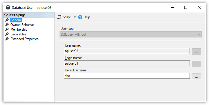
Figure 1. Database user based on a SQL Server login

To unlink this user from the SQL Server login, run the sp_migrate_user_to_contained stored procedure, specifying the database user that you want to migrate, as shown in the following example:

EXEC sp_migrate_user_to_contained   
@username = N'sqluser03',  
@rename = N'keep_name',  
@disablelogin = N'do_not_disable_login';

The sp_migrate_user_to_contained system stored procedure takes the following three parameters:

  • The @username parameter is the database user.
  • The @rename parameter determines whether to use the database user or the server login for the name. The keep_name value retains the database user name. The copy_login_name uses the login name.
  • The @disablelogin parameter determines whether to disable the login. In this case, the login will not be disabled. To disable the login, instead, specify the disable_login value.

After you run the EXECUTE statement, reopen the properties for the sqluser03 user. You’ll find that a login is no longer associated with the user and that the user type has been changed to SQL user with password, as shown in Figure 2.

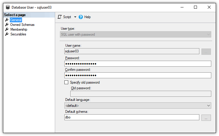
Figure 2. Password-based contained database user

When you unlink a database user from a login, SQL Server assign’s the login’s password to the user, as indicated in the figure. As a security best practice, you should reset the user’s password at this point. If you were to now rerun the following query, you should again receive the same rows from the ImportSales1 database:

EXECUTE AS USER = 'sqluser03'; 
SELECT * FROM ImportSales1.Sales.Customers;
REVERT;
GO

By unlinking the login from the database user, you can take full advantage of the portability inherent in contained databases. Be aware, however, that the sp_migrate_user_to_contained stored procedure works only for SQL Server logins and not Windows logins.

Securing SQL Server Contained Databases

Contained databases can make it easier to move a database from one SQL Server instance to another, without having to worry about duplicating login information between those instances. However, before implementing contained databases, you should be familiar with Microsoft’s security guidelines, described in the SQL Server help topic Security Best Practices with Contained Databases. The topic explains some of the subtler aspects of controlling access to contained databases, particularly when it comes to roles and permissions.

Aside from these guidelines, you’ll find that controlling access to a contained database works much like a non-contained database. You might need to duplicate users across multiple contained databases or unlink database users from their server logins, but these are relatively straightforward processes, much like controlling access in general. Once you understand the basics, you should have little trouble supporting more complex scenarios.

The post Introduction to SQL Server Security — Part 3 appeared first on Simple Talk.


from Simple Talk https://ift.tt/2EaIFyv
via

Thursday, February 21, 2019

Custom Forms in Bootstrap 4

Since the very beginning, Bootstrap managed to revamp and redecorate the visuals of HTML web pages. Bootstrap authors achieved that by extending the standard taxonomy of web elements in the various HTML specs with UX-oriented actionable and rendering elements as they emerged from the industry practices. The extended Bootstrap taxonomy includes elements such as modals, dropdowns, custom tooltips, navbars, tab strips, input and button groups, progress bars, carousels and more. None of these has a direct HTML match, but a smart combination of HTML templates, CSS styles and, in some cases, a pinch of JavaScript does the job.

In addition, Bootstrap resets the visual settings of pages changing the visual properties of a few native HTML elements. As a result, text input fields and buttons get rendered with color, padding and border settings different from browser’s standards. Needless to say, different Bootstrap themes apply different visual settings to the same set of native HTML elements.

Not all HTML constituent (visual) elements were originally affected by Bootstrap. Select lists, checkboxes, radio buttons, file uploads, special input fields (date/time field, range bars) were entirely left to the browser’s internal implementation. This created a visual gap between the elements touched by Bootstrap graphics and those left to the browser’s rendering. For this reason, a number of (mostly jQuery-based) plugins appeared to provide nicer graphics for select lists, checkboxes and radio buttons.

Finally, Bootstrap 4 brings the long-awaited restyling for core HTML elements. In this article, you’ll find out more.

Input Text Boxes

Let’s start with plain input text boxes. As mentioned, since the early days Bootstrap restyled input text boxes to give them a consistent look-and-feel. In version 4, an interesting new feature has been added in the form of a new CSS class.

<input readonly 
       type="text" 
       class="form-control-plaintext" 
       value="Some unmodifiable text" />

Typically, you give input text fields the class form-control to enable the Bootstrap restyling. However, if the input field is meant to be read-only, then by adding the new class form-control-plaintext you enable a different set of CSS styles that remove the surrounding frame typical of input fields. As a result, the content of the value property is rendered as plain text. The effective result is slightly different across browsers. In Microsoft Edge, the control is rendered as plain text. In Google Chrome, instead, the text is also sensitive to clicking, and a frame appears all around as a focus outline.

Checkboxes

Bootstrap 4 introduces the form-check-input class that, combined with form-check-label, improves the layout of plain checkboxes whether they are clickable or disabled. In particular, you use the canonical disabled attribute to disable the control, and Bootstrap will automatically apply a lighter color to indicate a different state. Depending on the specific needs of the user interface, multiple checkboxes may be rendered inline or vertically stacked. Both scenarios can be achieved through HTML layout elements (e.g., DIV elements) but using native Bootstrap 4 classes specifically targeted at checkboxes helps to gain consistency. Here’s how to render multiple checkboxes inline.

<div class="form-check form-check-inline">
    <input class="form-check-input" 
           type="checkbox" 
           id="c1" 
           value="c1">
    <label class="form-check-label" for="c1">First</label>
</div>
<div class="form-check form-check-inline">
    <input class="form-check-input" 
           type="checkbox" 
           id="c2" 
           value="c2">
    <label class="form-check-label" for="c2">Second</label>
</div>

As you can see, it’s all about wrapping checkboxes in a DIV container styled with the form-check class. In addition, you add the form-check-inline class to have controls laid out horizontally. Note that, by default, multiple checkboxes wrapped in form-check elements are stacked vertically. In other words, removing form-check-inline classes in the code snippet above will stack control vertically.

In all these cases, though, the actual user interface remains the one natively provided by the browser. A parallel set of classes also exists to modify the look-and-feel of checkboxes to make them look more modern and colorful. Here’s an example:

<div class="custom-control custom-checkbox">
     <input type="checkbox" 
             class="custom-control-input" 
             id="cc1" name="cc1">
     <label class="custom-control-label" 
            for="cc1">
            I'm a custom checkbox
     </label>
</div>

You use the classes custom-control and custom-checkbox on the surrounding DIV and custom-control-input and custom-control-label on the checkbox and the label respectively. The figure below (from Google Chrome) shows the difference between a default and a custom checkbox.

Bootstrap 4 allows making the checkbox a little bigger or a little smaller than the default by using the classes form-control-sm and form-control-lg on the surrounding DIV. Note that if you need larger checkboxes, then you’d better develop something yourself outside Bootstrap or get inspired by the tons of readymade snippets available online.

Radio Buttons

All aspects of default and custom checkboxes apply to radio buttons too. To have a radio button, you only have to change the value of the type attribute to radio. The figure below shows the user interface of Bootstrap 4 custom radio buttons.

Here’s the corresponding markup:

<div class="custom-control custom-radio">
     <input type="radio" 
            class="custom-control-input" 
            id="r1" 
            name="r1">
     <label class="custom-control-label" 
            for="r1">Option 1</label>
</div>
<div class="custom-control custom-radio">
      <input type="radio" 
            class="custom-control-input" 
            id="r2" 
            name="r2">
     <label class="custom-control-label" 
            for="r2">Option 2</label>
</div>

You may have noticed that the color of the checked radio button in the figure is different (orange) from the color of the checked checkbox seen earlier (blue). Blue is the default color of the Bootstrap classes, but it can be changed via CSS. Here’s how to make it orange.

.custom-radio 
.custom-control-input:checked~.custom-control-label::after {
    background-color: orange;   
    background-image: url(...); 
    border-radius: 50%;
}

The circle that characterizes the radio button is actually an SVG image identified by the provided URL. Here’s the SVG source of the default one.

<svg viewbox='-4 -4 8 8'>
    <circle r='3' fill='#fff'/>
</svg>

In the case of radio buttons, however, it holds the general recommendation to look elsewhere (e.g., http://bootsnipp.com) for fancier visual solutions.

Toggle Switches

Since the early days of iPhone devices, people loved the toggle switch UI element to choose between two mutually exclusive states—on/off, yes/no, true/false and the like. Conceptually, a toggle switch is not different from a single checkbox or perhaps two paired radio buttons. To make toggle switches attractive is their intuitive user interface. Many plugins and extensions to various frameworks have been created to make it easy to turn a checkbox into a toggle switch.

Since version 4.2, Bootstrap has its own class to render a custom checkbox as an iPhone-style toggle switch. Here’s the necessary markup.

<div class="custom-control custom-switch">
     <input type="checkbox" 
            class="custom-control-input" 
            id="accept">
     <label class="custom-control-label" 
            for="accept">I Accept</label>
</div>

The figure below demonstrates the toggle switch in its checked and unchecked state.

In addition to making it a custom checkbox, the only class to use is custom-switch. Again, note that you need at least Bootstrap 4.2. The latest version at the time of this writing is 4.3.

Drop-down Lists

In the newest Bootstrap version, the SELECT element got a minor restyling at last. It’s nothing comparable to multi-select, highly customizable drop-down lists you can find around. One of the most commonly used is Bootstrap Select. You can download and play with it here.

Natively from the core Bootstrap, you get the following user interface only a bit nicer than the default one rendered by browsers.

The corresponding markup is shown below. As you can see, the only change you’re required to introduce is the custom-select class.

<select name="food" class="custom-select">     
    <option selected>No favorite food</option>     
    <option value="meat">Meat</option>     
    <option value="fish">Fish</option>     
    <option value="vegan">Vegan</option> 
</select>

The drop-down fully supports the multiple selection in the usual HTML way, that is by adding the multiple attribute.

File Uploaders

The file uploader component has always been part of the HTML specification since the very early days. Lately, though, it is often hidden behind nicer user interfaces that support the drag-and-drop of files and preview of images. Some basic restyling of the classic input box with a push button that unifies the rendering across all browsers is possible.

<div class="custom-file">
     <input type="file" 
            class="custom-file-input" id="file1">
     <label class="custom-file-label" for="file1">
          Choose file
     </label>
</div>

The classes custom-file, custom-file-input, and custom-file-label do the job of restyling the file uploader. Bootstrap 4 also allows you to change the label that describes the purpose of the file. The Choose file description of the code snippet above can be replaced by simply editing the body of the LABEL element. Also, the text of the button can be changed or localized, but that requires recompiling the Bootstrap SASS sources.

This said, the file uploader—even restyled—doesn’t seem to be the preferred choice of developers today. Not because there’s more to improve, but because drag-and-drop and preview (and even data binding) are must-have features.

Range Inputs

Introduced by HTML5, the range input controls provide a way for users to enter a number in a closed range. The default user interface of a range control in Google Chrome is below:

As mentioned, the user interface changes with the browser. Bootstrap 4 provides additional CSS classes to give range controls a uniform interface across browsers. Here’s how to turn it on.

<div> 
     <label for="customRange">Your age?</label>
     <input type="range" 
            class="custom-range" 
            id="customRange" 
            name="range1" />
</div>

The trick is using the class custom-range on the INPUT element of type range. The output is shown below, and it is uniform across browsers.

In this case, the highlight color (blue by default) can be changed via CSS, as shown earlier for checkboxes.

More Specific Form Control Classes

In Bootstrap 4, you also find a number of additional form-control-XXX CSS classes that apply to the rendering of a variety of INPUT elements, as listed in the table below.

In addition, for all INPUT elements in a Bootstrap 4 form, you can set heights using classes like form-control-lg and form-control-sm.

Form Sizing

In Bootstrap 4, forms also support auto-layout for columnar content. On the foundation of flexbox grids, developers can set the width of one column using the col-N syntax and then have the sibling columns automatically adapt to the remaining width. In other words, the remaining columns (out of a total of 12 available in the grid system) are equally split on the remaining space. The flexbox grid works regardless if predefined grid classes (e.g., col-6) or inline widths are used: the remaining columns will resize accordingly. The class col indicates that the width of the column is flexibly adapted. Here’s a sample form that lays out horizontally, with the first column taking up half the width and the remaining two a quarter each.

<form>
    <div class="form-row">
       <div class="col-6">
            <input type="text" class="form-control">
       </div>
       <div class="col">
           <input type="text" class="form-control">
       </div>
       <div class="col">
           <input type="text" class="form-control">
       </div>
    </div>
</form>

Summary

An interesting trend is going on in the web industry and revolves around the use of custom components in web pages. In this context, a custom component is a reusable set of HTML tags encapsulated in a single container. As a result, the new component can be used within web pages as if it were a native part of the markup language. Whether part of an Angular, React, or a Blazor solution, web components extend the taxonomy of a web page.

Bootstrap attempted to do the same since the first version. Unlike web components, though, Bootstrap didn’t introduce any new top-level syntax element in the HTML markup but provided a number of HTML snippets that altogether worked as a new component.

Until version 4, Bootstrap disregarded a number of fundamental HTML elements (e.g., checkboxes, radio buttons, select menus) that only now are styled in a modern and consistent, non-browser-based way. This article just covered custom forms as they’re supported in Bootstrap 4.

The post Custom Forms in Bootstrap 4 appeared first on Simple Talk.


from Simple Talk https://ift.tt/2E15t3z
via

Applied AI in Software Development

Artificial Intelligence (AI) has been in the limelight in recent years with self-driving cars, its most famous application. Although experiments with AI began in the 1950s, the latest advancements in machine learning proves it’s emerging as a disruptive technology. Several companies in a variety of domains are trying to find ways to utilize AI agents or bots to automate tasks and improve productivity. Software testing is no different. A wave of automation has already hit software testing in the form of Automation Testing.

The automation of quality assurance and software testing has been around for over 15 years. Test automation has evolved from automation of test execution to using model-based testing tools to generate test cases. This evolution was primarily triggered by shifting of focus from reducing testing timelines to increasing test coverage and effectiveness of testing activities. However, the level of automation of software testing processes are still very low due to two main reasons:

  • Difficulty to develop scalable automation to match the speeds of the changing applications with every release
  • Challenges with architecting a reliable and reusable test environment with relevant test data

This is going to change with the adoption of AI, analytics, and machine learning in testing. This article will explain what AI is, dispel some widespread myths, and establish some ground realities regarding its current capabilities.

What is AI?

Artificial Intelligence is an application of individual technologies working in tandem which helps a computer to perform actions usually reserved by humans. Some of the common applications of AI in our daily lives are speech recognition and translation in the form of bots like Siri and Alexa and autonomous vehicles, including self-driving cars as well as spacecraft. When you consider these applications of AI, you will notice that each of these are very specialized functions. The primary limitation of the technology right now is that it is not generalized; meaning, implementation of AI which can do all the things above like a human being doesn’t exist yet.

During the early periods of AI development, scientists and researchers understood that it is not necessary for them to emulate the human mind completely to build autonomous learning or make computers think. Instead, they are working on ways to model the way we perceive inputs and act on them. This makes sense because the very hardware that our human brain runs on is different from the hardware in our computers. This is also the reason why we keep hearing analogous terms like neural nets which have been modeled from our understanding of how the neurons work in our brains. However, researchers will tell you that this model is oversimplified and perhaps doesn’t match reality at all. This shows that we are still far from the likes of developing Skynet (for the Terminator fans) or Ultron (from the Marvel universe) to rest some predictions from doomsayers that AI is an existential risk for all humans. For now, we are safe, unless we give AI access to our nuclear codes for them to use.

What Makes AI Possible?

In the previous section, I spoke of some individual technologies which work together to make AI possible. Now, I’ll explain in detail what these technologies are. Since the 1950s, AI has been experimented with in various forms by fields like computational linguistics for natural language processing, control theory to find the best possible actions, and machine evolution or genetic algorithms to find solutions to problems. However, with the advent of the information age and the decrease in the cost of computational power & memory, all these technologies have found common ground as machine learning.

Machine Learning is essentially the way in which we are making computers learn and perceive the world. There are primarily three main ways, computers learn:

  • Supervised Learning
  • Unsupervised Learning
  • Reinforcement Learning

Supervised Learning

In supervised learning, a computer is provided with labeled data so that it can learn what distinguishes each feature. For example, to make the computer distinguish you from your partner, you need to provide a set of photos distinctly marked as such. This set of marked/labeled input is then provided to an algorithm for the computer to create a model. This model is later used by the computer to distinguish whether photos that are provided to it are from you or your partner. This is a simple case of classification. Another example would be to use insurance data to predict the range of losses the company could make from the insurance product, given a set of attributes of a person. Supervised learning is thus usually used for classification or regression problems.

Unsupervised Learning

Unlike supervised learning where labeled data is available, unsupervised learning tries to find patterns in the input provided on its own. This method of learning is used in a lot of applications like clustering (grouping similar objects together and finding point of separation between distinct ones), association (finding relations between objects) and anomaly detection (detecting unnatural behavior in the normal operation of a system).

Reinforcement Learning

Reinforcement learning is the closest method which is making AI agents possible. In this method of learning, the AI agent explores the environment and finds an optimal way to accomplish the goals. It uses an iterative process to perform actions, receive feedback because of those actions and an evaluation of the feedback to see if the action was positive or negative. Reinforcement learning also uses models created using supervised and unsupervised learning to evaluate or perform actions.

AI in Testing

Now that you know the capabilities of AI and have a better understanding of what goes behind the creation of AI, you’ll see how AI is impacting software testing. AI in testing refers to one of these things:

  • AI-enabled testing
  • Testing AI products and deliverables

AI will enable enterprises to transform testing into a fully self-generating, self-executing, and self-adapting activity. Although the use of AI in testing is still in initial phases in the industry, software testing tools have started implementing some or the other forms of AI in their toolkit. Tools like Eggplant and TestComplete have some AI features in their latest releases.

The main objectives with any QA or testing efforts are to:

  • Ensure end-user satisfaction
  • Increase the quality of software by detecting software defects before go-live
  • Reduce waste and contribute to business growth and outcomes
  • Protect the corporate image and branding

Hence with testing AI products and deliverables, the software tester could use traditional testing tools, or use AI-enabled testing tools. The primary objectives remain the same; however, one now needs considerable understanding and knowledge of the workings of AI algorithms to find new ways to break the application.

Currently, AI-enabled testing comes in three different flavors.

Predictive Analytics

Predictive analytics in software testing is simply the use of predictive techniques like object detection and identification to perform steps in test execution. Prominent tools like Eggplant and TestComplete have now introduced such features in the latest releases. You will see an example of this feature in detail later.

Robotic Automation

Robotic automation or Robotic Process Automation (RPA) is a technique to automate repetitive processes which require no decision making. This is more analogous to macros in Excel applied to an entire lifecycle rather than just a simple task. Some of the components of this technique are screen scraping, macros, and workflow automation.

Cognitive Automation

Cognitive automation is a level up on RPA which also introduces machine learning to automate software testing phases. Thus, providing decision-making capabilities to the tool. Cognitive automation is still a work in progress and you should expect to see more tools and products adopting this approach soon.

Now that you have gained an understanding of the capabilities of AI and its implications in testing, take a look at some examples of how testing tools are utilizing AI to empower testers.

An example of AI in testing

Automation tools gained prominence across the software industry aiming to reduce repetitive manual work, increase efficiency and accuracy of test execution, and perform regular checks by scheduling jobs to run on a release schedule. With the coming of AI, there are various tools available in the market which are adopting this technology, one of the most widely used tools is TestComplete. It can be used to automate mobile, desktop and web applications and supports the creation of smoke, functional, regression, integration, end-to-end, and unit test suites. It provides the functionality to record test cases or create them in various supported scripting languages such as C# Script, C++Script, DelphiScript, JavaScript, JScript, Python, VBScript. Recorded test cases can also be converted into scripts. Take a look at how the traditional steps in software testing are carried out in TestComplete.

Test Creation and Execution

There are multiple approaches supported by TestComplete for creating and executing the test cases. Record and play options are available to record step by step user interactions with an application, and then it can be played multiple times as needed. Once the test case has been recorded, multiple conditions can be added as follows:

  • Using statements supported by TestComplete to perform iterative actions & conditions, e.g. while, if…else, try catch & finally etc.
  • Passing runtime parameters during the execution
  • Creating variables and passing it in test scripts
  • Performing different actions on the selected object such as clicking on the button, entering text, opening and closing the application.
  • Adding various property validation checkpoints such as reading and validating a label of any object, finding its location, checking whether it is enabled or disabled, etc.

Once the test cases are created and ready to be executed, following options can be used to execute them:

  • Running test cases individually using the Run Test option.
  • Creating separate functions in the script file and deciding which function to run under the Project Suites gives more flexibility for tester
  • You can also rearrange the sequence of the test cases to be executed under the project. Another way is to add them under a specific folder and then decide which one to execute
  • You can also call scripts written in any language into the keyword test cases which provides more flexibility.
  • You can also execute an entire project suite by selecting the entire project suite and choosing the option Run Project .

What’s the Role of AI

When it comes to validating the property of an object present on the UI, TestComplete provides multiple options to access the object’s properties. For example, a button object can have properties like enabled or disabled, text, coordinates, Id, class, etc. Hence, it becomes easy to identify an object based on these properties and confirm the expected behavior. However, reading content on images or a graphical chart like interfaces which are becoming more common with the proliferation of business intelligence and data-driven dashboards is difficult to identify and validate or perform automated actions on them. However, this has changed with the introduction of the latest version of TestComplete viz. version 12.60 which overcomes this issue by making use of an API driven optical character recognition (OCR) service.

There are certain prerequisites to use this option. First, one needs to enable the OCR plugin by installing the extension under File –> Install Extension. Second, since it makes use of the ocr.api.dev.smartbear.com web service, firewall proxy settings should be enabled to access this web service.

There are two main ways in which this feature can be utilized:

  • Keyword tests In Keyword tests, one basically uses the two operations, OCR Action and OCR Checkpoint
  • Script tests For script tests, a tester would need to access the OCR object to invoke functions and properties

I’ll demonstrate the power of the new service with the help of two testing scenarios below.

Testing a Dashboard

Application Description: A Tableau dashboard contains an analysis of tweets with the hashtag #TCEurope18. It contains three elements, (Figure 1.1)

  • Textbox named User Screen Name
  • Horizontal bar chart “Who had the most tweets?”
  • Scatter plot “Whose retweets were more popular?”

You can filter the data using the User Screen Name filter textbox. Upon filtering data from the textbox, the horizontal bar chart Who had the most tweets? and the scatter plot Whose retweets were most popular? should both get updated as per the filtered value.

Also, selecting a bar on the bar chart should filter, the scatter plot for the same user.

Figure 1.1

Test Scenario#1

On selecting a bar from the bar chart Who had the most tweets?, the scatter plot Whose retweets were most popular should also show the plot for the same user (validating username).

Initial stage: all the usernames and the metrics are displayed on both the charts


Record a step to click on the bar chart to select username datakmart to view data related to the datakmart user:

In the expected result it should display the username datakmart in both the graphs and confirm the same by reading the text from the graphs:

Now add a property checkpoint to read the username from both the graphs using the OCR option.

TestComplete reads the value from the graph and displays in the OCR section, you can select which value you want to use for the validation. The following image shows values from the horizontal bar chart Who had the most tweets?:

The following image shows values that TestComplete has captured from the Whose retweets were most popular? scatter plot graph:

This is how your recorded keyword test case will look. It has two checkpoints with the name OCR Checkpoint in the test:

Test Scenario #2

Providing an input to the User Screen Name should filter the data in both the charts for the same input(username).

Initial stage: all the usernames and the metrics are displayed on both the charts (Figure 1.2)

Figure 1.2

Record a step to click on the User Screen Name textbox, enter the text tableau, hit the enter button and click on the checkbox for the tableau option from the filter drop-down:

Now verify that both the graphs display the data for the same filtered text, i.e., tableau by adding property checkpoints:

This is how your keyword test case will look:

Test execution result:

The AI feature you saw demonstrated in the above cases are examples of the Hybrid Object Detection feature. Another example of this feature is to test outputs in PDF files. Here’s an example of testing PDF outputs.

For this test, use a test PDF with addresses as below which is an output of a process.

So same as before, start recording and select the PDF object.

A screenshot of a social media post Description automatically generated

This selects the object as above. Click Next.

Select OCR, which will parse the PDF and recognize the text on the PDF. The recognized text will be displayed in the Recognized text field as below.

A screenshot of a social media post Description automatically generated

You can provide the text to find in the recognized text for satisfying the test criteria. You could also use patterns as well for a wildcard search.

Now that you have seen the examples of Hybrid Object Detection, here’s an example of the Intelligent Recommendation system.

TestComplete uses the Intelligent Recommendation system to detect objects in the Name Mapping repository. You can switch on the feature to add objects to the Name mapping repository automatically. This can also be utilized for dynamically searching and mapping objects. This comes in handy to maintain test cases for applications that change object positions in the object hierarchy. This dynamic behavior is common during state changes at various points in time during the application execution. The recommendation system helps automatically map objects across the object hierarchy based on the object properties.

These are some good examples of the application of machine learning models for software testing. TestComplete also has a provision to use external packages for Python and other scripting languages which can be leveraged to include other machine learning models for object detection, translation, audio to text, etc.

Conclusion

With the evolution of test automation from test execution & functional testing to a more lifecycle automation approach, it is imperative that robotic automation and cognitive automation will become a norm in the market soon. Machine learning & AI are game changers and testers should expand their skills to exploit the opportunities.

References


The post Applied AI in Software Development appeared first on Simple Talk.


from Simple Talk https://ift.tt/2SOzaix
via

Wednesday, February 20, 2019

Protecting Data During Development

In the years before joining Redgate, I was a SQL Server database consultant. I spent a lot of time doing SQL Server health checks, query tuning, and ETL (extract, transform, and load) development. Every customer was different and getting to the resources I needed to do the job at each shop varied as well. I usually had to remote into a server or virtual workstation and work with a development database.

Providing databases for developers and database professionals is not easy, and there are several decisions to make. You must decide if all members of the team will share a dev database or if each member will have their own copy. Will these databases reside on a development server or will they live locally on developer workstations? You may also have to provide databases for QA and test. Even having enough disk storage for all these databases, often including multiple versions and backups, can be a challenge.

The data in the non-production databases should resemble production data. Imagine a query that runs blindingly fast on 100 rows of test data but is miserably slow against production tables where millions of rows are queried. Often the simplest thing to do is to give developers backups of the production databases for development. This becomes impossible as databases approach terabyte sizes, but there is another issue. Copies of production databases could contain sensitive information that should be protected like names and addresses, health insurance claims, or credit cards. The developers should not see this data, and nightmare scenarios like lost laptops holding private data happen all too frequently.

Private data given to developers must be obfuscated in some way, and it must be obscured enough so that identities can’t be figured out by looking at clues in the data and putting the pieces back together. And protecting this data is not just a nice thing to do. Regulations like GDPR and HIPAA as well as new or proposed legislation in the individual US states have steep penalties for failing to protect private data. Database administrators must have processes in place to protect sensitive data and to make sure that it does not make its way onto non-production servers.

I remember spending so much time pulling down backup files and restoring databases after every sprint a few years ago at some of my customer engagements. I never seemed to have enough storage space on my virtual desktops, either. It was quite the time-consuming juggling act. Luckily, today there are some tools that can help solve these problems like Redgate’s SQL Provision. The DBAs can create masking sets to obfuscate sensitive data, create an image, and then allow developers to provision their own clones. These clones take up a few megabytes of space on the developer’s workstation, and it just takes seconds to create the clone once the image is in place. Working with the clones is just like working with a regular database. Everything can be automated with PowerShell, saving time and protecting the data after every sprint.

Providing data to developers is not easy unless you have the proper tools. Technologies like database cloning and masking can ensure that developers have databases that resemble production but without the sensitive data and without taking up a lot of precious space or time. Protecting sensitive data is serious business, but having the right tools can make it less painful and more efficient.


The post Protecting Data During Development appeared first on Simple Talk.


from Simple Talk https://ift.tt/2GBgrAI
via

The BI Journey: The Expert’s Advice – Part 1

The series so far:

  1. The BI Journey: The Analyst
  2. The BI Journey: The Expert’s Advice – Part 1

When Ruthie started her internship at AdventureWorks, the famous bicycle and accessories seller, she sparked off a business intelligence solution that even surprised her (The BI Journey: The Analyst). All she did was build a “dashboard” for her boss Stephen, the Sales Manager. Stephen found much value in the solution that Ruthie gave him, even trying to create his own reports from the data. The secret of this was the flexible semantic model that Ruthie had built. A semantic model, if built correctly, provides a business-centric, user-friendly, flexible interface of organizational data to the end user. Some of the credit was due to advice from George, the local analytics guy who works with the technology community. It was George who guided Ruthie to create a solution that was better than the first iteration with tips and advice on designing the solution and how to better present the data to the users.

A Typical Analyst’s Dataset

When George looked at the dataset that Ruthie had given him, the first thought that went through his head was “Gosh! Not a typical analyst’s dataset!” It was one big fat table that had all the columns that needed to go into the report. While it was good if one was running an analytical algorithm such as a forecasting model, it was painful when performing self-service analysis and George hated it. However, he thought that it was great that Ruthie had at least cleaned it up the way she had by only including columns that needed to be analyzed (facts) and the columns that were needed to perform the analysis of these facts (dimensions). He explained to Ruthie that what she had done was great for performing different types of analysis quickly and easily. He told her that her design gives way to a modeling technique called dimensional modeling.

However, he also told her that, if more sources such as the sales targets Excel file was needed to be correlated with sales, things can get a little complicated. He proceeded to explain more about modeling data for analysis.

The sales table’s structure looked like what’s in Figure 1

Figure 1: Sales table

There are many types of analyses that can come from any combination of columns from this table. For example, Ruthie or Stephen could use it to look at the factual data, order value, broken down by product category as in Figure 2:

Figure 2: OrderValue by ProductCategory

Another analysis that they could perform might be order value for each product category purchased by each customer broken down by year (Figure 3).

Figure 3: OrderValue by ProductCategory by Customer by Year

Correlating order value and order quantity throughout the months as in Figure 4 could also be another type of analysis that can be performed.

Figure 4: OrderValue and OrderQty by Month

However, George explained that in order to perform analysis in a flexible and efficient manner, a more structured technique had to be employed to construct the data structure. Facts and Dimensions

The first thing about creating a data structure that works well for analysis is to identify which columns are the ones that are going to be measured (facts), and which columns are going to determine the context or perspective of what was to be measured (dimensions).

Identifying facts is quite straight forward George explained to Ruthie; just ask the business, or as a business user you would probably know. Even if you weren’t a business user, you could still probably identify a lot of the columns that can be categorized as facts. These are usually numeric such as order value, quantity sold, call handling time, exam score, etc. Then, you need to identify the dimensions. These would be columns such as product, product category, date, and customer. These are quite easy to identify as well. However, the thing that you need to ensure is that columns that are not useful should not be taken into account. For instance, the product category is a great way of analyzing sales orders, whereas modified_by is not. Additionally, in many cases, groups of dimension columns can be identified as a single dimension. For instance, product, product subcategory, and product category can all be grouped up into the product dimension.

Figure 5: Sales Orders table

All in all, if you can divide your columns into facts and dimensions, and put up a diagram such as this, you are on the right path for proper analytics.

Figure 6: Sales dimensional model

Ruthie wasn’t convinced at first and thought that George had just split her table up into a fancy diagram. How was that even useful? George had agreed somewhat but told her to think of a scenario where you would need to analyze by year when all you have is the date column. Ruthie was quite familiar with Power Query by then. She responded that all you needed to do was to create a custom column or duplicate the date column and transform it to a year. Date and year can be grouped to be made into the calendar dimension according to George’s theory. It still hadn’t seemed compelling why a diagram such as the “dimensional model” had to be drawn. George had smiled, Ruthie was a fast learner, and he had her where he wanted her.

Dimensional Modeling

George then pulled up the Excel file that Stephen had shared, which had sales targets for the last few years. Stephen had wanted these targets to be correlated against the sales numbers. However, the granularity of the targets was different from that of the sales data, which was what George had wanted to point out to Ruthie to explain why the fancy dimensional model was needed.

He asked a simple question: since sales values are from one table and targets are from another, if you needed to compare them against each other, which table’s salesperson would you use? Or which table’s product categories would you use? Ruthie answered without thinking; use each table’s respective salesperson and product category columns. George smiled and explained that if the sales table’s product categories were used to measure the sales values, and the target table’s product categories were used to measure the sales targets, they will only be measured separately, and a correlation or comparison of the two would not happen.

To view the correlation between measures from two tables, you need to have common dimensions. And that is why it makes sense to pull dimensions out into their own tables, and then link them to the fact tables. The only column that would remain in the fact tables would be the column that makes up the grain. If you pull out product categories, you naturally need to pull out product subcategory and product. However, you need to leave the product column (or the product ID if it is available) in the fact table as well so that a link can be made to the products table. If there is only one column in a dimension, then the column can be left as it is, and there is no need for a separate dimension table. But life almost always has more columns (also called attributes) to a dimension.

In short, George said, the columns that belong to each dimension needed to be pulled out, leaving only the lowest most level of that dimension. Going back to Ruthie’s query, he showed her how they should look:

Figure 7: Sales table (stripped off dimension columns)

Each of the following columns, CustomerID, SalespersonID and Product ID should connect to their respective tables, Customer, Salesperson and Product (Figure 8, Figure 9 and Figure 10). He said that Ruthie should not worry about dates yet, and the OrderDate column can be used for dates, months and years because of the automatic hierarchy that Power BI generates for date columns.

Figure 8: Customer dimension table

Figure 9: Salesperson dimension table

Figure 10: Product dimension table

George showed Ruthie the relationship tab and explained that product + customer + salesperson + date was the detailed level of data in the model. Moreover, for every combination of the grain that exists there should be one record, and that is why Power BI summarizes the rest of the columns. This structure, he said, was called a star schema due to its shape (Figure 11).

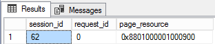
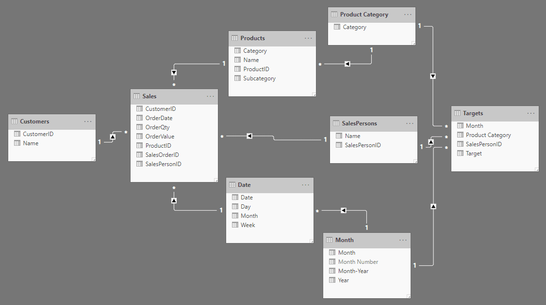
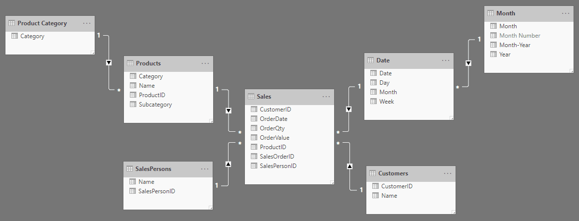
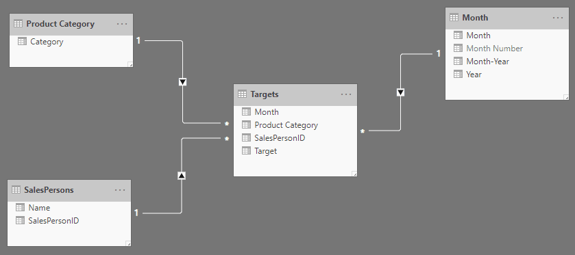
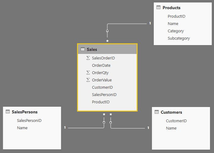
Figure 11: The sales dimensional model

Granularity

Then comes the issue of different granularity. The granularity of sales was product + customer + salesperson + date, while the targets’ granularity was product category + salesperson + month. Which means sales values and targets could be correlated at a higher level, but that would not be the case at a lower level. For example, you could get the total sales for 2018, and the total target values for 2018 and perform a comparison. Whereas, when you drill down to a lower level, for instance, to the product level, there won’t be any target values to show, because targets exist only up to the product subcategory level, which brings us to a dilemma.

Finally, Ruthie understood what all this fancy modeling meant. She reckoned that “being technical” was just a stigma that people put on others so that they didn’t have to do that job. However, all it takes was understanding the basics and the need to provide value to whomever you worked for, and you realize that most things are not that technical at all.

Ruthie was quickly able to create a dimensional model combining sales and targets: all it took was understanding the organization’s data and the basics of modelling.

She pulled in the Excel file for targets given to her by her boss Stephen.

Figure 12: Targets spreadsheet

She then mashed it up with her existing data model, using the principles taught to her by George.

Figure 13: Dimensional model with Sales and Targets with different granularities

To compare the sales with its targets, but due to the difference in granularity, Ruthie split out the Products table by moving the category to its own table but keeping the link. So now, she can analyse the sales by products all the way to the category, and at the same time analyze targets alongside at the category level. She also created Date and Month tables and did the same.

This was what the sales portion looked like without targets:

Figure 14: Sales star (snowflake) schema

Since the product category was pulled out of Products, and the Month table was separated out from Date, the star was now a snowflake.

This was what the targets portion looks like without sales:

Figure 15: Targets star schema

Each of these star schemas, when put together make up the dimensional model in Figure 13.

Semantic Model (or Layer)

George told Ruthie that one of the most important things about modeling data for analysis was interfacing the data to the business user in the most business-centric way. To do this, one needs to apply a semantic layer on top of the dimensional model. This semantic layer can be almost the same as the dimensional model, or it can be much more sophisticated. The semantic layer (or semantic model) takes the dimensional model and applies business logic and business formatting on top of it. This is where measures and KPIs used by a business are created. For instance, business logic can be applied on top of the sales value fact by writing a calculation to generate the month-to-date cumulative sales value, or a calculation using both the sales value and the sales target to come up with the sales achievement ratio.

George showed how to create a simple measure on top of the data model. He said that before you create sophisticated measures, even the least sophisticated ones, you needed to first create the basic measures. These basic measures would be just the facts with an aggregation calculation wrapped around them. Then if dragged onto a visual on a report, the aggregated fact and a basic measure would work more or less the same.

He showed how to create a measure, and how it looked a lot like using Excel functions. Something that business users and analysts, those who swear by Excel, would love to see:

Revenue = SUM(Sales[OrderValue])

Figure 16 shows how the measure looks inside the model.

Figure 16: Creation of the Revenue measure

He explained that even if the measure appeared under the Sales table, it was because the Sales table had been selected when the measure was created, and that a measure can be placed in any table as long as it made sense.

He quickly demonstrated how the measure (Revenue) and the column that made it up (OrderValue) when placed on a visual behaved the same:

Figure 17: OrderValue (column) vs Revenue (measure)

“Then, why would you want to have measures?” was Ruthie’s obvious question. Well, that’s the first step before you create more complex measures on top of it, and what complex measures can do, in most cases cannot be done by mere columns, explained George.

He explained by taking an example: If you had the following data set how would you calculate the growth of sales?

Region

Last Year

This Year

Growth

A

500

490


B

550

720


C

470

710


D

390

585


Figure 18: Sales example data set

The calculation you would use in the Growth column would be:

([This Year] – [Last Year])/[Last Year]

The result:

Figure 19: Sales example data set with growth calculation

Now, when you want the entire sales for last year, and the entire sales for this year, naturally it would be a sum of each column, where Last Year would yield 1910 and This Year would yield 2505. But when you need the growth for the entire year, summing up the Growth column and coming up with 1.3 (130%) is wrong. You would have to instead perform the same calculation on the totals of each column and come up with 0.312 (31.2%). This would hold true to at whatever level that you choose to perform an aggregation. You will have to perform the aggregations first and then do the calculation, instead of performing the calculation first and then performing the aggregations, and that’s just what a measure does.

Under George’s guidance, Ruthie created the following measures off sales and target facts:

Units = SUM(Sales[OrderQty])
Target Units = SUM(Targets[Target])

And then she created the following measure on top of these measures to analyze the target achievement ratio:

Achievement % = CALCULATE([Units]/[Target Units])

All in a Day’s Work

Ruthie felt a great deal of contentment after all the learning and the work that she had put in. She spent some time playing around with the model she had built. She put up different visuals, dragged in the measures she had created along with the other columns and tried out different analyses. The more she tried it out, the more ideas she got for additional types of analysis. She started thinking about bringing in more data points. For example, what if she could bring in website log files which had information on page hits? That way she could correlate page hits for the different product pages with that of sales and see if the AdventureWorks website actually played a part in boosting sales. The possibilities seemed endless, but first, she had to perfect the current model. There was so much that could be done with the current data set alone.

She stopped working for the day. Tomorrow she would perfect the model as best as she could, and then start applying the rest of the best practices and advice that George had suggested. She would also try to include Stephen’s suggestions as well.

As Ruthie found out with her session with George, all sorts of analysis can be performed on data, as long as the semantic model is built well. To have a well-built semantic model, the underlying data set should be modeled in the most flexible way possible; this is where dimensional modeling comes into play. With a little bit of technicality, business analysts can go a long way to provide value with data.

The post The BI Journey: The Expert’s Advice – Part 1 appeared first on Simple Talk.


from Simple Talk https://ift.tt/2txFe02
via