Cracking DAX – the EARLIER and RANKX Functions

The series so far:

1. Creating Calculated Columns Using DAX
2. Creating Measures Using DAX
3. Using the DAX Calculate and Values Functions
4. Using the FILTER Function in DAX

If you really want to impress people at DAX dinner parties (you know the sort: where people stand around discussing row and filter context over glasses of wine and vol-au-vents?), you’ll need to learn about the EARLIER function (and to a lesser extent about the RANKX function). This article explains what the EARLIER function is and also gives examples of how to use it. Above all, the article provides further insight into how row and filter context work and the difference between the two concepts.

Loading the Sample Data for this Article

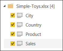
As for the other articles in this series, the sample dataset consists of four simple tables which you can download from this Excel workbook:

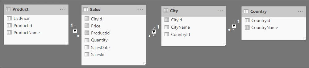
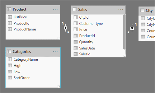
After importing the data, you should see this model diagram (I’ve used Power BI, but the formulae in this article would work equally well in PowerPivot or SSAS Tabular):

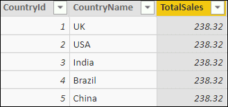
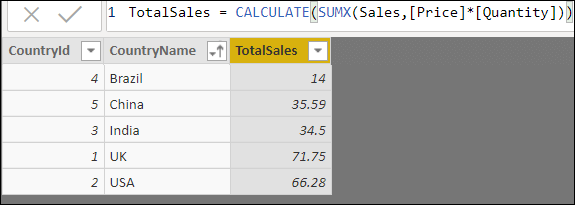
One more thing to do – add a calculated column to the country table, giving the total sales for each country:

TotalSales = CALCULATE(Sumx(Sales,[Price]*[Quantity]))

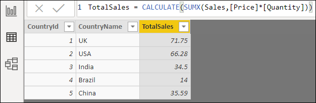
This formula iterates over the Sales table, calculating the sales for each row (the quantity of goods sold, multiplied by the price) and summing the figures obtained. The CALCULATE function is needed because you must create a filter context for each row so that you’re only considering sales for that country – without it, you would get this:

Example 1: Ranking the Countries

The first use case is very simple. The aim is to rank the countries by the total sales for each:

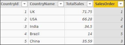
DAX doesn’t have an equivalent of the SQL ORDER BY clause, but you can rank data either by using the RANKX function (covered later in this article) or by using the EARLIER function creatively. Here’s what the function needs to do, using country number 3 – India – as an example. Firstly, it creates a row context for this row:

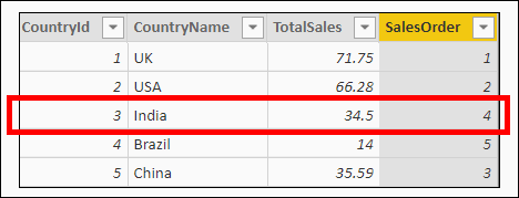
The sales for India are 34.5. What it now must do is to count how many rows there are in the table which have countries whose sales are greater than or equal to India’s sales:

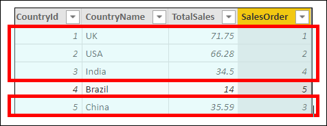
This shows the filtered table of countries, including only those whose sales are at least equal to India’s. There are four rows in this filtered table.

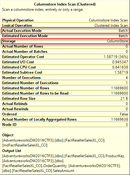
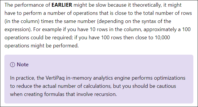
If you perform the same calculations for each of the other countries in the table, you’ll get the ranking order for each (that is, the number of countries whose sales match or exceed each country’s). For those who know SQL, this works in the same way as a correlated subquery. This would imply that it might run slowly, however, here’s what Microsoft have to say on the subject:

The problem: One Row Context Hides Another

Anyone who has driven much in France will have seen this sign at a level-crossing:

What it means is “one train can hide another” … and so it is with row contexts. The measure will open two row contexts, as the diagram below shows:

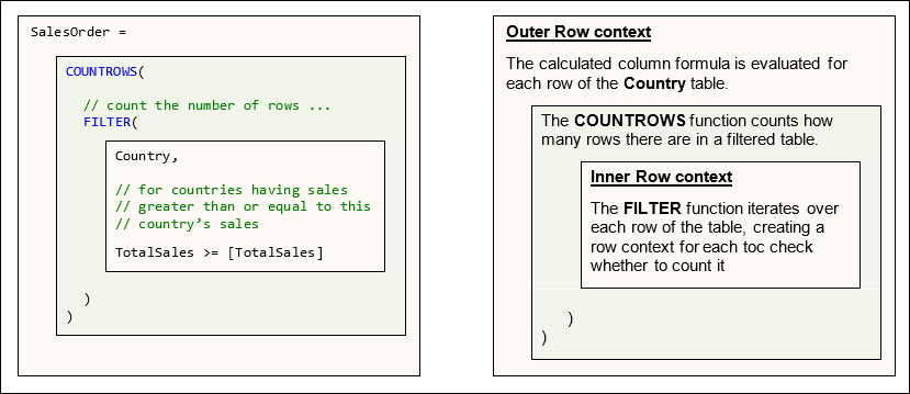
The problem is that when DAX gets to the inner row context for the FILTER function, it will no longer be able to see the outer row context (the country you’re currently considering) as this row context will be hidden unless you use the EARLIER function to refer to the first row context created in the formula.

What Would You Name this Function?

I’ve explained that the EARLIER function refers to the original row context created (nearly always for a calculated column). What would you have called this function? I’d be tempted by one of these names:

• OUTERROWCONTEXT
• PREVIOUSROWCONTEXT
• INITIALROWCONTEXT

The multi-dimensional (cubes) version of Analysis Services gets it about right, using CURRENTMEMBER and PREVMEMBER depending on context. It’s interesting to see that you can’t use these words as names of variables in DAX as they are reserved words:

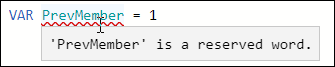
This is true even though they aren’t official DAX function names!

What I definitely wouldn’t use for the function name is something which implied the passage of time. To me, EARLIER means something which occurred chronologically before something else. I think this is one of the reasons it took me so long to understand the EARLIER function: it’s just got such an odd name.

The Final Formula Using EARLIER

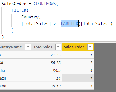
Having got that off my chest, here’s the final formula:

SalesOrder = COUNTROWS(
    Filter(
        Country,
        [TotalSales] >= EARLIER([TotalSales])
   )
)

Here’s the English (!) translation of this …

“For each country in the countries table, create a row context (this happens automatically for any calculated column). For this row/country being considered, count the number of rows in a separate virtual copy of the table for which the total sales for the country are greater than or equal to the total sales for the country being considered in the original row context”.

What could possibly be confusing about that?

Other Forms of the EARLIER Function

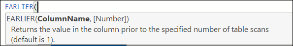
Readers will be delighted to know that you don’t have to limit yourself to going back to the previous row context – you can specify how many previous row contexts to return to by varying the number used in the second argument to the EARLIER function:

You can even use the EARLIEST function to go to the earliest row context created for a formula. The formula could alternatively have been written like this:

SalesOrder = COUNTROWS(
    FILTER(
        Country,
        [TotalSales] >= EARLIEST([TotalSales])
    )
)

I find it very hard to believe that anyone would need this function! It could only be useful where you:

1. Create a row context (typically by creating a calculated column).
2. Within this, create a filter context.
3. Within this, create a row context (typically by using an iterator function like FILTER or SUMX).
4. Within this, create another filter context.
5. Within this, create a third-row context.

In this complicated case, the EARLIER function would refer to the row context created at step 3, but the EARLIEST function would refer to the original row context created at step 1.

Avoiding the EARLIER Function by Using Variables

One of the surprising things about the EARLIER function is that you often don’t need it. For this example, you could store the total sales for each country in a variable, and reference this instead. The calculated column would read instead:

Sales order using variables = 
// create a variable to hold each country's sales
VAR TotalSalesThisCountry = [TotalSales]
// now count how many countries have sales 
// which match or exceed this
RETURN COUNTROWS(
    FILTER(
        Country,
        [TotalSales] >= TotalSalesThisCountry
    )
)

There’s not much doubt that this is easier to understand, but it won’t give you the same insight into how row context works!

Using the EARLIER function in a measure

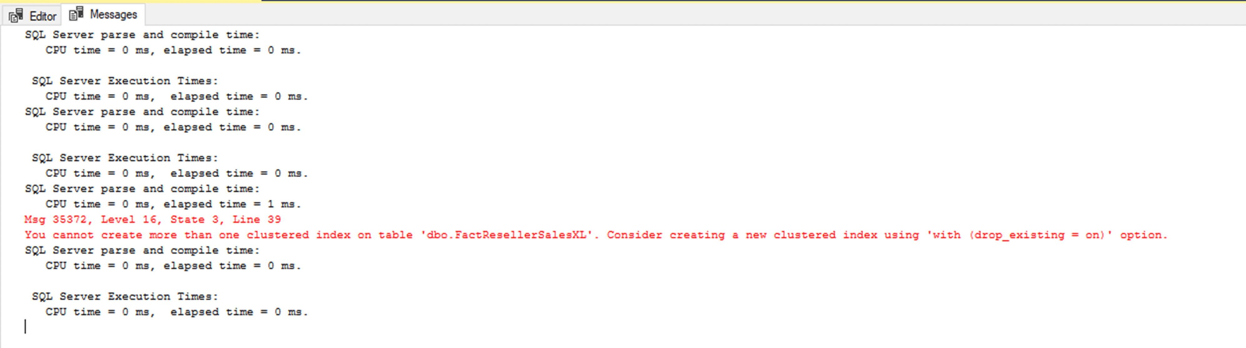
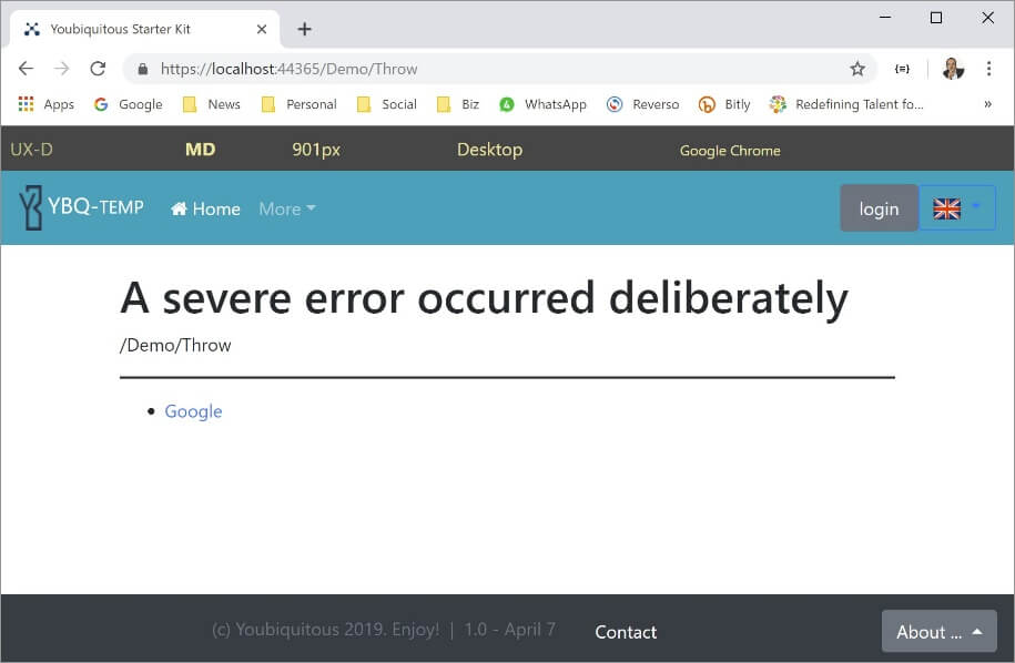
The EARLIER function refers to the previous row context created in a DAX formula. But what happens if there isn’t a previous row context? This is why you will so rarely see the EARLIER function used in a measure. Here’s what you’ll get if you put the formula in a measure:

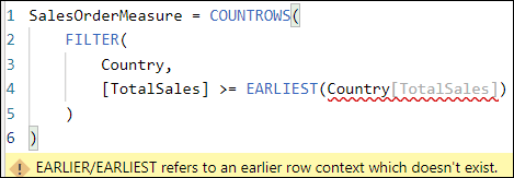
The yellow error message explains precisely what the problem is: measures use filter context, not row context, so no outer row context is created.

Example 2: Running Totals

Another common requirement is calculating the cumulative total sales for countries in alphabetical order:

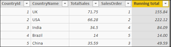
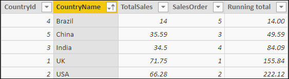
The above screenshot shows that this calculates the answer separately for each country, but it looks more sensible when you view it in alphabetical order by country name:

The formula for this column calculates for each country the total sales for all countries coming on or before it in alphabetical order:

Running total = SUMX(
    FILTER(
        Country,
        Country[CountryName] <= EARLIER(Country[CountryName])
    ),
    [TotalSales]
)

Again, you could have alternatively used a variable to hold each country’s name:

Running total using variables = 
// store this row's country name
VAR ThisCountry = Country[CountryName]
// return the sum of sales for all countries up to or
// including this one
RETURN SUMX(
    FILTER(
        Country,
        Country[CountryName] <= ThisCountry
    ),
    [TotalSales]
)

Example 3: Group Totals

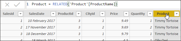
Here’s another use of the EARLIER function – to create group totals. To follow this example, first, add a calculated column in the Sales table to show the name of each product bought (you don’t have to do this, but it will make the example clearer if you use the product name rather than the product id to match sales rows to the product bought):

Product = RELATED(‘Product'[ProductName])

Here’s the column this should give:

You can now create a second calculated column:

Average product sales = AVERAGEX(
    
    // average over the table of sales records for the 
    // same product as this one ...
    FILTER(Sales,[Product] = EARLIER(Sales[Product])),
    
    // ... the total value of the sale
    [Price]*[Quantity]
)

Here’s what this will give for the first few roles in the SALES table. You may want to format the column as shown by modifying the decimal places on the Modeling tab.

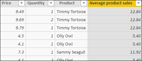
The group average for Olly Owl products is 5.40. For this example, for each sales row, the calculated column formula is averaging the value of all sales where the product matches the one for the current row.

Example 4: Creating Bands

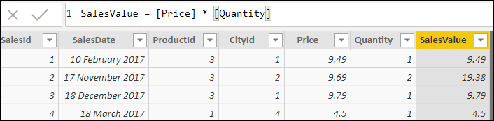
So far, you have seen three relatively simple uses of the EARLIER function – for the fourth example, I’ll demonstrate a more sophisticated one. Begin by adding a calculated column to the Sales table, giving the value of each transaction (which should equal the number of items bought, multiplied by the price paid for each):

It would be good to categorise the sales into different bands, to allow reporting on different customer bands separately. For example:

• Any purchase with value up to £10 is assigned to “Low value”
• Any purchase with value between £10 and £15 is assigned to “Medium value”
• Any purchase with value between £15 and £20 is “High value”
• Any purchase of more than £20 is “Premium customer”

One way to do this would be to create a calculated column using a SWITCH function like this:

Customer type = SWITCH(
    // try to find an expression which is true
    TRUE(),
    // first test - low value
    [SalesValue] <= 10, "Low value",
    // second test - medium value
    [SalesValue] <= 15, "Medium value",
    // third test - high value
    [SalesValue] <= 20, "High value",
    // otherwise, they are a premium customer
    "Premium customer"
)

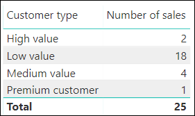
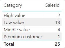
This would allow reporting on the different customer types (for example, using this table):

However, this hard-codes the thresholds into the calculated column. What would be much more helpful is if you could import the thresholds from another table, to make a dynamic system (similar to a lookup table in Excel, for those who know these things).

Creating the Table of Bands (Thresholds)

To create a suitable table, in Power BI Desktop choose to enter data in a new table (you could also type it into Excel and load the resulting workbook):

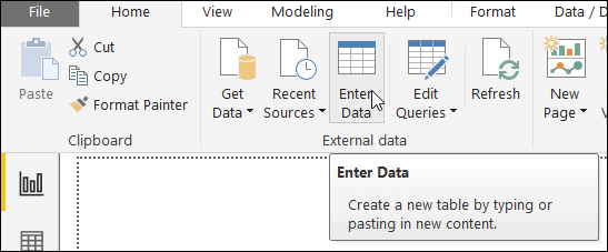
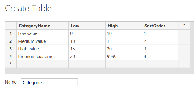
Type in the thresholds that you want to create, and give your table the name Categories:

Note that in your model’s relationship diagram, you will now have a data island (a table not linked to any other). This is intentional:

Creating a Formula Assigning Each Sale Row to a Category

You can now go to the Sales table and create a calculated column assigning each row to the correct category:

For each row, what you want to do is find the set of rows in the Categories table where two conditions are true:

The lower band for the category is less than the sales for the row; and

The upper band for the category is greater than or equal to the sales for the row.

It should be reasonably obvious that this set of rows will always exist, and will always have exactly one row in it. Because of this, you can use the VALUES function to return the value of this single row, giving:

Category = CALCULATE(
    // return the only category which satisfies both of
    // the conditions given
    VALUES(Categories[CategoryName]),
    // this sales must be more than the lower band ...
    Categories[Low] < EARLIER(Sales[SalesValue]),
    // ... and less than or equal to the higher band
    Categories[High] >= EARLIER(Sales[SalesValue])
)

You might at this point wonder why you need the EARLIER function when you haven’t created a second row context. The answer is that the CALCULATE function creates a filter context, so you need to tell your formula to refer back to the original row context you first created in the formula.

Sorting the Categories

One problem remains: the categories aren’t in the right order (I’m well aware that one way to solve this would be to click on the column heading to change the sort order, but I’m after something more dynamic!):

To get around this, it may at first appear that all you need to do is to designate a sort column:

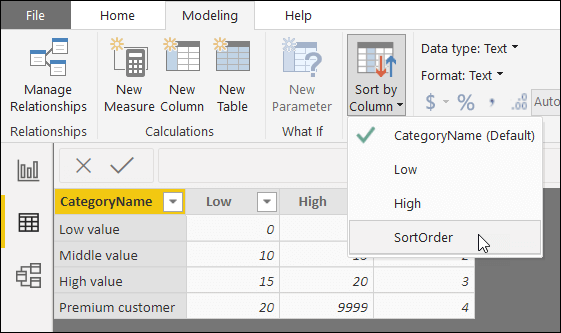
You could do this by selecting the CategoryName column in the Categories table as above, and on the Modeling tab, setting this to be sorted by the SortOrder column. This looks promising – but doesn’t work (it actually creates an error if you’ve typed in the data for the categories table, which you’ll need to refresh your model to clear). The reason this doesn’t work is that the alternative sort column needs to be in the same table as the Category column.

A solution is to create another calculated column in the Sales table:

Category SortOrder = CALCULATE(
    // return the sales order for the two conditons
    VALUES(Categories[SortOrder]),
    // this sales must be more than the lower band ...
    Categories[Low] < EARLIER(Sales[SalesValue]),
    // ... and less than or equal to the higher band
    Categories[High] >= EARLIER(Sales[SalesValue])
)

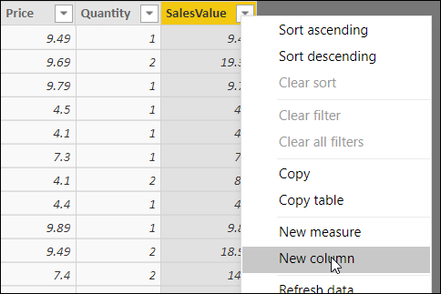
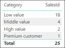
You now have two columns for each sale row – one giving the category, and one giving its corresponding sort order number. You can select the category column and choose to sort it using the sort order column instead (choosing the option shown below on the Power BI Modeling tab):

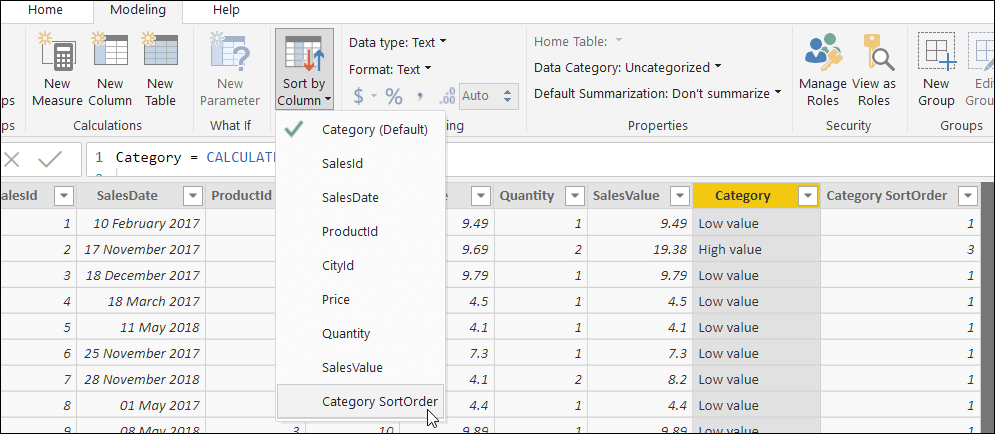
Bingo! The categories appear in the required order:

If after reading this far you’re still a bit fuzzy on the difference between row and filter context, practice makes perfect! I’ve found reading and re-reading articles like this helps, as each time you get closer to perfecting your understanding (for those in the UK, you could also consider booking onto one of Wise Owl’s Power BI courses).

Using the RANKX Function to Rank Data

Out of all the DAX functions, the one which trips me up most often is RANKX – which is odd, because what it does isn’t particularly complicated. Here’s the syntax of the function:

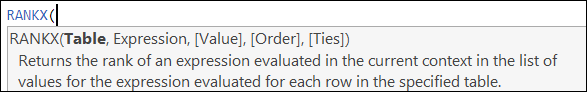
So the function ranks a table by a given expression. Here is what the arguments mean:

• The Table argument gives the table you’re ranking over.
• The Expression argument gives the expression you’re ranking by.
• The Order column allows you to switch between ascending and descending order.
• The Ties column lets you specify how you’ll deal with ties.

You’ll notice I’ve missed out the Value argument. This is for the good reason that it is a) bizarre and b) not useful. It allows you to rank by one expression, substituting in the value for another for each row in a table. If this sounds like a strange thing to want to do, then I’d agree with you.

To see how the RANKX function works, return to the Country table in which you created a calculated column at the beginning of this article:

Suppose you now want to order the countries by sales (clearly one way to do this would just be to click on the drop arrow next to the column and choose Sort ascending!). Here’s a calculated column which would do this:

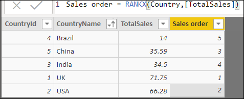
What you should notice is the unusual default ranking order: unlike in SQL (and many other languages), the default order is descending, not ascending. To reverse this, you could specify ASC as a value for the fourth Order argument:

Sales order = RANKX(
    
    // rank the rows in the country table ...
    Country,
    
    //... by the total sales column ...
    [TotalSales],
    
    // omitting the third argument
    ,
    
    // and ranking in ascending order
    ASC
)

So far, so straightforward!

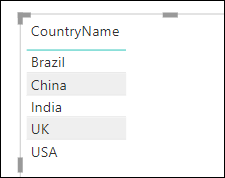
Using RANKX in a Measure

Where things get more complicated is when you use RANKX in a measure, rather than in a calculated column. Suppose that you have created a table visual like this in a Power BI report:

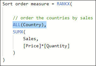
Suppose further that you want to create and display this measure to show the ranking order:

Sort order measure = RANKX(
    // order the countries by sales
    Country,
    SUMX(
        Sales,
        [Price]*[Quantity]
    )
)

However, when you add this measure to your table, you get this:

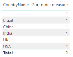
The reason for this is that Power BI evaluates the measure within the filter context of the table. So for the first row (Brazil), for example, here’s what Power BI does:

• Applies the filter context to the Country table to pick out just sales for Brazil
• Calculates the total sales for this country (14, as it happens)
• Returns the position of this figure within the table of all of the figures for the current filter context (so the returned number 1 means that 14 is the first item in a table containing the single value 14)

To get around this, you first need to remove filter context before calculating the ranking order, so that you rank the total sales for each country against all of the other country’s total sales:

However, even this doesn’t solve the problem. The increasingly subtle problem is that the RANKX function – being an iterator function – creates a row context for each country, but then evaluates the sales to be the same for each country because it doesn’t create a filter context within this row context. To get around this, you need to add a CALCULATE function to perform context transition from row to filter context within the row context within the measure:

Sort order measure = RANKX(
    // order across ALL the countries ...
    ALL(Country),
    // by the total sales
    CALCULATE(
        SUMX(
            Sales,
            [Price]*[Quantity]
            )
        )
    )

This – finally – produces the correct ranking (note that there is a blank country at the top because some sales don’t have a matching country parent – although this isn’t important for this example):

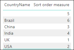
It’s worth making two points about this. Firstly, this isn’t a formula you’ll often need to use; and secondly, this is about as complicated a DAX formula as you will ever see!

Dealing with Ties

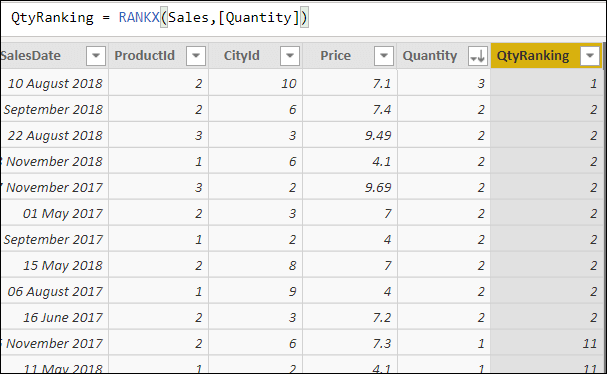
If your ranking produces ties, the default is to SKIP numbers, but you can also use the DENSE keyword to override this. To see what each keyword means, add this calculated column to the Sales table:

QtyRanking = RANKX(Sales,[Quantity])

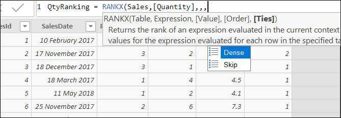
What it will do is to order the sales rows by the quantity sold. Here’s what you’ll get if you use Skip, or omit the Ties keyword altogether:

Here, by contrast, is what you’ll get if you use Dense (I’m not quite sure why you’d ever want to do this):

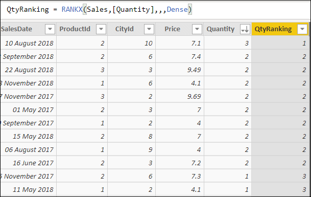
In the second screenshot, there are no gaps in the numbers.

Conclusion

You can apply the EARLIER function in various contexts to solve modelling problems in DAX, and it should be an essential part of every DAX programmer’s arsenal. The RANKX function, by contrast, solves a very specific problem – ranking data. What both functions have in common is that they are impossible to understand without a deep understanding of row and filter context, so if you’ve got this far, you can consider yourself a DAX guru!

The post Cracking DAX – the EARLIER and RANKX Functions appeared first on Simple Talk.

from Simple Talk https://ift.tt/2yoEKf7
via

ASP.NET Core 3.0 Exception Handling

An aspect of the ASP.NET Core platform that I have loved since the first version is that the team attempted to engineer some of the common best practices of previous ASP.NET development right in the framework. This is particularly evident for exception handling.

When it comes to dealing with the things that could go wrong in your application, the big issue is not using try/catch blocks wherever it makes sense, but making sure you can effectively trap whatever exception that could be thrown but may go unnoticed and unhandled by the application. Since the early days of programming (remember Visual Basic’s OnError?), it’s always been a good practice to define a sort of a safety net around the application to intercept whatever exception bubbles up outside the control of the calling context.

In this article, I’ll explain the facts of exception handling as you would set it up in ASP.NET Core 3.0.

The ASP.NET Safety Net

Whether Web Forms or MVC, classic ASP.NET provides a global error handler function in the folds of the global.asax file—the Application_Error method. Any code you use to fill the method is invoked just before the system displays the nefarious yellow page of death or lets the web server deal with an error HTTP status code. In other words, the code you put in the body of the Application_Error method represents your last chance to fix things before the end.

What kind of code should you have, however, in a global error handler?

Intelligently, classic ASP.NET let us define error paths in the web.config file and uses those paths to re-route the user to a different page. The path you specify is ultimately a URL and, as such, can point to a static or even a dynamic endpoint. A static endpoint (e.g., an HTML page) can’t do much for the end-user but profoundly apologise for the (largely unknown) error. A dynamic endpoint (an ASPX file or a controller route) can, in theory, tailor an up-close-and-personal message but only if it can gain access to the specific situation that generated the error.

In years of ASP.NET programming, we have first learned how to retrieve the last occurred exception and redirect back to the most appropriate error page. This ultimately resulted in a flexible error router dispatching to a myriad of error pages. The sore point of global exception handling, in fact, is that you discover the error in one request but need to place another request to the system to have the error message rendered in a user-friendly and nice-looking error page. The Server.TransferRequest method was introduced for that purpose. The method works like a canonical redirect except that it takes place internally and no interaction ever takes place with the browser. In addition to that, in ASP.NET MVC you can even find a way to place an analogous internal URL request that the action invoker stack would process as if it were originated by an external request. As a result, you get an exception, and then some code of yours runs with full access to the details of the exception and the power to display some user interface at leisure.

In the end, building a safety net around the application was a problem solved in ASP.NET and ASP.NET MVC. In ASP.NET Core, the way you address it is different and passes through a new type of middleware.

The Exception Handling Middleware

In ASP.NET Core 3.0, you install the exception handling middleware and let it capture any unhandled exceptions and redirect to the most appropriate endpoint. As mentioned, the redirect isn’t physical—no HTTP 302 request is ever sent—but logical, and the browser is never involved with this.

There are two types of exception handling middleware: one is targeted to developers and is ideal for development scenarios, and one is suitable for staging and production environments and, as such, targeted to end-users.

In a development scenario, you might want to have the original error message displayed, and you even want the stack trace available and a snapshot of the HTTP context with details of the query string, session state, cookies and the like. This is just the kind of thing labelled as the “yellow page of death” in older versions of ASP.NET.

To have that, you append the following piece of middleware to the ASP.NET Core runtime pipeline. In startup.cs, you add the following:

app.UseDeveloperExceptionPage();

As you can see, the middleware is parameter-less and doesn’t allow routing to a custom page or view. The middleware, instead, prepares a system page on the fly that contains the details of the last intercepted exception and a snapshot of system status at the time of the exception. It’s a terminating middleware in the sense that it stops the request and represents the new “white page of death”—yes, they changed the background colour!

Hand in hand with this middleware, you can also use the UseExceptionHandler middleware that, instead, is ideal for production-ready exception handling.

The UseExceptionHandler Middleware

You add the UseExceptionHandler middleware to the pipeline using the Configure method of the startup class. Here’s an example:

public class Startup
{
    public void Configure(IApplicationBuilder app)
    {
        app.UseExceptionHandler("/system/error");
        ...
    }
}

The UseExceptionHandler extension method takes a URL and logically redirects the flow of the application to it. More in detail, the middleware places a new request for the specified URL right into the ASP.NET pipeline.

As the two middleware blocks address distinct scenarios—one for development and one for production—you might want to programmatically switch between middleware at runtime. You just use the services of the hosting environment API.

public void Configure(
      IApplicationBuilder app, IHostingEnvironment env)
{
    if (env.IsDevelopment())
    {
        app.UseDeveloperExceptionPage();
    } 
    else 
    {
        app.UseExceptionHandler("~/system/error");
    }
    ...
}

The methods of the IHostingEnvironment interface let you detect the current environment and intelligently decide which exception middleware to turn on. Based on the listing above, the Error method on the System controller is invoked to deal with any unhandled exceptions.

The next point to address is, what should you do when an exception is thrown and travels unhandled up to the safety net?

Handling the Exception

Looking at the code snippet above, the Error method is invoked without explicit parameters. In the past, the GetLastError method on the Server intrinsic object helped to retrieve the last exception occurred. No such object exists anymore in ASP.NET Core, but the new Features property on the HTTP context object allows to retrieve runtime information such as the last exception occurred and related information. Here’s the code you need to have in the global error handler.

public IActionResult Error()
{
    // Retrieve error information in case of internal errors
    var error = HttpContext
              .Features
              .Get<IExceptionHandlerFeature>();
    if (error == null)
         return View(model);

    // Use the information about the exception 
    var exception = error.Error;
    ...
}

You query the HTTP context of the current request for the latest exception and receive an object that implements the IExceptionHandlerFeature interface. The object exposes a single property named Error which points you right to the last tracked exception.

The interesting part is that once you hold in your hands a valid exception object, then you have all the available information about what could have gone wrong and can arrange the most appropriate response—whether some plain text or a full-blown, nice-looking error page. You can also decide to swallow most of the details contained in the exception object and route to a few of the predefined (and more generic) error message. In other words, you’re now in total control of what you display to your users.

You are so much in control that you could even throw an exception any time that a business operation goes wrong or can’t be performed for whatever reason. Instead of returning error codes all the way up, from the inner layers to the presentation, you throw an exception, and you’re done. To gain even more control, you can, for example, build your own hierarchy of exception objects, specific to the application. (I’ll return on this in a moment.)

Referencing the Request

The IExceptionHandlerFeature interface only returns information about the exception that was thrown at some point but nothing about the URL in the execution of which the exception threw. To get that, you need to request the IExceptionHandlerPathFeature interface to the HTTP context object, as shown below.

public IActionResult Error()
{
    // Retrieve error information in case of internal errors
    var path = HttpContext
              .Features
              .Get<IExceptionHandlerPathFeature>();
    if (path == null)
         return View(model);

    // Use the information about the exception 
    var exception = path.Error;
    var pathString = path.Path;
    ...
}

Note that the IExceptionHandlerPathFeature interface inherits from the aforementioned IExceptionHandlerFeature meaning that with a single request you get both the exception and path information.

What About 404 Errors?

The safety net captures any exceptions whether they originate in the processing of the request or the preparation of it, such as during model binding or in case of a missing route. With the approach shown earlier, however, you can’t get to know about the specific HTTP status code returned by the pipeline without an exception being thrown. The most notable example is a 404, but also any request that returns an error HTTP code such as 500.

To be sure your code can handle any HTTP status code of interest, you should add another piece of middleware to the pipeline.

app.UseStatusCodePages();

The status code middleware is another terminating middleware that directly returns some output to the end-user. In particular, it writes a plain text string to the output stream with the error code and the basic description. To handle the HTTP status code programmatically, you need another piece of middleware on top of the exception handler.

App.UseStatusCodePagesWithReExecute("/system/error/{0}");

The parameter {0} will be set with the HTTP status code if any. The re-execute in the name of the method just denotes that the request that generated a response with an error status code will be logically redirected (re-execute means no 302 to the browser) to the specified URL. Here’s how to rewrite the method to display the above error page to the user.

public IActionResult Error(
     [Bind(Prefix = "id")] int statusCode = 0)
{
    // Switch to the appropriate page
    switch(statusCode)
    {
        case 404:
           return Redirect(...);
        ...
    }


    // Retrieve error information in case of internal errors
    var path = HttpContext
              .Features
              .Get<IExceptionHandlerPathFeature>();
    if (path == null)
         return View(model);

    // Use the information about the exception 
    var exception = path.Error;
    var pathString = path.Path;
    ...
}

The HTTP status code is received through the model binding layer, and, if it matches one of those, the method can handle it and select the appropriate action. Note that the way in which the status code parameter is bound to the method is up to you. The approach shown above of using an id parameter is only an example.

Going One Step Further

How would you arrange the error page? Aside from some standard graphical template, what would you put in it? For sure, you want to render some message, whether the native message of the caught exception or some other more generic message. Anything else you would do?

Personally, I tend to have two levels of messages in any exception and a list of recovery links. The first level message is the native message of the exception (or any other programmatically selected message related to the error occurred). The second level message is any other descriptive message you might optionally want to display.

A recovery link, instead, is an application URL (or even an external URL) that you add to the error page to let users resume with the application from one or more safe places. Typically, one recovery link can be the home page. Recovery links should be bound to each exception type so that you specify them by the time you throw.

The idea is to set a base exception type on a per-application basis. For example, you can have a MyAppException base class as below:

public class MyAppException : Exception
{
   public MyAppException()
   {
       RecoveryLinks = new List<RecoveryLink>();
   }
   public MyAppException(string message) : base(message)
   {
       RecoveryLinks = new List<RecoveryLink>();
   }
   public MyAppException(Exception exception) : 
                      this(exception.Message)
   {
   }
   public List<RecoveryLink> RecoveryLinks { get; }
   public MyAppException AddRecoveryLink(
           string text, string url)
   {
        RecoveryLinks.Add(new RecoveryLink(text, url));
        return this;
   }
   public MyAppException AddRecoveryLink(RecoveryLink link)
   {
        RecoveryLinks.Add(link);
        return this;
   }
}

The RecoveryLink class is a custom class with a couple of properties—text and URL. Any other application-specific exception will inherit from MyAppException and will have available handy methods to deal with recovery links.

public IActionResult Throw()
{
    throw new MyAppException("A severe error occurred")
        .AddRecoveryLink("Google", "http://www.google.com");
}

In the exception handler, you just try to cast the exception object retrieved to MyAppException. If successful, you can then access the recovery links and use them in the user interface.

<ul>
@foreach(var link in Model.Error.RecoveryLinks)
{
    <li><a href="@link.Url">@link.Text</a></li>
}
</ul>

FIGURE 1-A sample error page using exception handlers and recovery links.

Summary

When it occurs, an exception breaks the normal flow of execution of a program and causes a re-routing. If you foresee that something could go wrong at some specific point, then the best option is probably using a try/catch block to wrap the risky code. However, sometimes, exceptions occur inadvertently and having a safety net around the application is quite useful. In this article, I’ve reviewed the ASP.NET Core 3.0 equipment for global error handling and suggested a couple of improvements for smoothing exception handling in real-world applications.

The post ASP.NET Core 3.0 Exception Handling appeared first on Simple Talk.

from Simple Talk https://ift.tt/2SMH9cD
via

PolyBase in SQL Server 2019 – The End of ETL?

One of the new features in SQL Server 2019 is SQL Server Big Data Clusters, and one part of this feature is PolyBase. Now you may wonder: Hasn’t PolyBase been around for quite a while? And you’re right! PolyBase was introduced in SQL Server 2016 and is also a key feature in Azure SQL Data Warehouse to bring in data from flat files sitting on an HDFS Cluster. It treats these sources as external tables which you can query through T-SQL just like any local table stored in your SQL database.

So, what’s new then? In SQL Server 2019, Microsoft greatly enhanced the capabilities of PolyBase. Instead of only flat files, you can now bring in data residing on other relational and non-relational data sources such as other SQL Servers, Oracle, Teradata or MongoDB.

Microsoft is using PolyBase – a technology which has been around since SQL Server 2016 – to deliver a solution for data virtualisation.

Data integration has been accomplished in the past by using tools like SSIS, PowerShell, bcp and others to copy data from one data source to another. Data virtualisation allows the data to be queried at its original source. This means that any query against such data becomes a real-time query while at the same time, it avoids the redundancy of storing data in two places. From a user perspective, a query against a PolyBase table is no different than against a regular table so you may also offload and switch local tables into external tables at some point without breaking any queries. Such a change can, of course, imply substantial positive or negative performance impacts.

One potential use case would be offloading older data to cheaper storage and servers or even to Azure while still having it accessible within your central data hub through PolyBase.

What will I need to do to use the new PolyBase capabilities?

First, you will need an installation of SQL Server 2019, which is currently in the Customer Technology Preview (CTP) phase. You can download the latest preview here.

During the installation, you must also add the PolyBase feature:

PolyBase also requires the Java Runtime Environment 8 (JRE) as a prerequisite, so it must be in place before installing SQL Server 2019. If you plan to use PolyBase against a Teradata source, you will need the C++ Redistributable 2012 also.

If you are using Chocolatey, you can install both tools using these two lines in a command prompt:

choco install jre8 -y
choco install vcredist2012 -y

In the PolyBase Configuration screen, you can decide between a standalone as well as a scale-out option. Both will work, however the standalone option is recommended unless you have a specific interest or need in the additional installation overhead that comes with scale-out.

Once the installer has finished, connect to your SQL Server instance to enable Polybase. This is done through a small T-SQL script:

exec sp_configure @configname = 'polybase enabled', @configvalue = 1;
RECONFIGURE

TCP-IP must also be enabled. Be sure to review the PolyBase installation instructions for more information. After enabling the feature, restart your SQL Server instance. PolyBase is now ready to use.

OK, I got it installed. But how do I use it? How can I query another SQL Server?

Once you connect a table from another server using PolyBase, you’ll see the table listed just as if the table was local. The table is read-only, however, and has the word “External” next to the name when viewing from ADS. At this time, you won’t see the tables in the Object explorer in SSMS, but you can still query them from that tool.

To add a table from another SQL Server as a PolyBase source to your database, you will need a master key (to encrypt credentials), credentials to connect to the other database (PolyBase only supports simple authentication), the external data source itself (server- and database name) as well as the definition of the table(s) you want to add.

While you can achieve all this through T-SQL, the easiest way is to make use of the external table wizard in Azure Data Studio (ADS). To get the wizard, you will need to add the SQL Server 2019 extension for Azure Data Studio. Follow the instructions on the download page to perform the installation.

Note that at the time of this writing, you must change the downloaded file’s extension from .zip to .vsix.

Before getting started, make sure that the source instance is using mixed-mode and set up a SQL Server login with read permission to the table you will link.

To open the wizard, connect to the instance running PolyBase and the database where you want to see the external table. Right-click the user database and select “Create External Table.”

The wizard will first prompt you to confirm the destination database and pick a data source. While PolyBase in SQL Server 2019 supports a wide range of external sources like Teradata or DB2, the Wizard currently only supports SQL Server and Oracle. There is another wizard for flat files. All others will need manual scripting. In this case, select SQL Server.

As SQL Server will store the usernames and passwords required to connect to the external data sources, these need to be encrypted. This requires a master key to be set on the source database which will be taken care of by the wizard if no key exists yet:

In the next step, you need to provide a server as well as a database name. Supply a name for the new Credential and add the login and password that you created. This will link the login to the new Credential which will be used to connect to the source instance.

If you have created such a connection and credentials before, you can re-use them by picking their respective entry from the select box:

Now that you have a connection to the external server, the wizard will get a list of all tables and views included in the respective source database. You can either select specific tables/views or all of them:

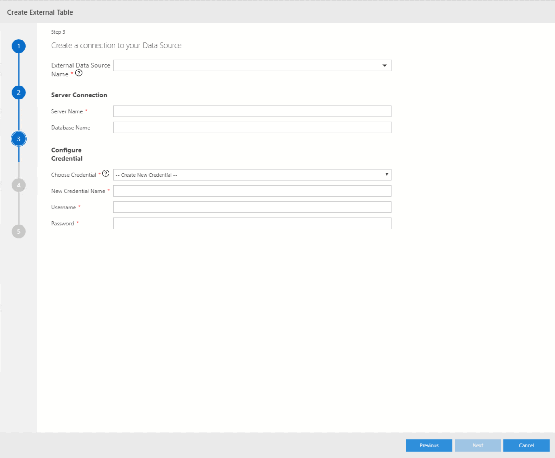
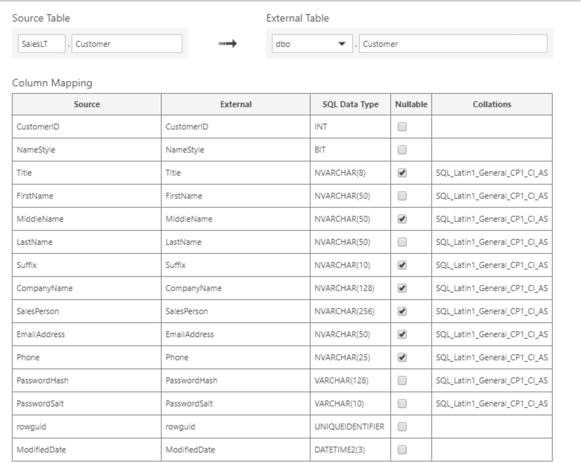
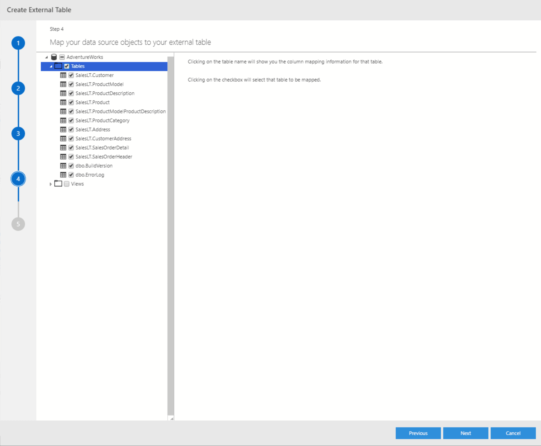
For each table, you can change the schema as well as the table name itself which will be used for the external table as shown in the next figure. To get to this screen, just click in the respective table name in the list. You cannot change data types or column names, nor can you only select specific columns. While this may seem confusing to begin with, it doesn’t matter as no actual data is being transferred at this point. That will only happen later when querying the table, and at this point, your SELECT statement will determine which columns are about to be used.

In the end, the wizard will give you a summary as well as the option to either generate everything that you’ve just defined or to create a script which you can manually execute at any later point in time:

You can also complete all the steps using T-SQL. In this example, I have just brought in the Customer table for an AdventureWorksLT database in Azure SQLDB:

BEGIN TRY
    BEGIN TRANSACTION Tf86fd76a5b6a42f3a5fb144c4c0713f
        EXEC('USE [PolybaseSample]');
        CREATE MASTER KEY ENCRYPTION BY PASSWORD = N'Password';
        CREATE DATABASE SCOPED CREDENTIAL [AW]
            WITH IDENTITY = N'Username ', SECRET = N'Password';
        CREATE EXTERNAL DATA SOURCE [AW]
            WITH (LOCATION = N'sqlserver://YourServer', CREDENTIAL = [AW]);
        CREATE EXTERNAL TABLE [dbo].[Customer]
        (
            [CustomerID] INT NOT NULL,
            [NameStyle] BIT NOT NULL,
            [Title] NVARCHAR(8) COLLATE SQL_Latin1_General_CP1_CI_AS,
            [FirstName] NVARCHAR(50) COLLATE SQL_Latin1_General_CP1_CI_AS NOT NULL,
            [MiddleName] NVARCHAR(50) COLLATE SQL_Latin1_General_CP1_CI_AS,
            [LastName] NVARCHAR(50) COLLATE SQL_Latin1_General_CP1_CI_AS NOT NULL,
            [Suffix] NVARCHAR(10) COLLATE SQL_Latin1_General_CP1_CI_AS,
            [CompanyName] NVARCHAR(128) COLLATE SQL_Latin1_General_CP1_CI_AS,
            [SalesPerson] NVARCHAR(256) COLLATE SQL_Latin1_General_CP1_CI_AS,
            [EmailAddress] NVARCHAR(50) COLLATE SQL_Latin1_General_CP1_CI_AS,
            [Phone] NVARCHAR(25) COLLATE SQL_Latin1_General_CP1_CI_AS,
            [PasswordHash] VARCHAR(128) COLLATE SQL_Latin1_General_CP1_CI_AS NOT NULL,
            [PasswordSalt] VARCHAR(10) COLLATE SQL_Latin1_General_CP1_CI_AS NOT NULL,
            [rowguid] UNIQUEIDENTIFIER NOT NULL,
            [ModifiedDate] DATETIME2(3) NOT NULL
        )
        WITH (LOCATION = N'[AdventureWorks].[SalesLT].[Customer]', DATA_SOURCE = [AW]);
    COMMIT TRANSACTION Tf86fd76a5b6a42f3a5fb144c4c0713f
END TRY
BEGIN CATCH
    IF @@TRANCOUNT > 0
        ROLLBACK TRANSACTION Tf86fd76a5b6a42f3a5fb144c4c0713f
    DECLARE @ErrorMessage NVARCHAR(4000) = ERROR_MESSAGE();
    DECLARE @ErrorSeverity INT = ERROR_SEVERITY();
    DECLARE @ErrorState INT = ERROR_STATE();
    RAISERROR(@ErrorMessage, @ErrorSeverity, @ErrorState);
END CATCH;

Isn’t that the same thing, as a linked server?

At first sight, it sure looks like it. But there are a couple of differences. Linked Servers are instance scoped, whereas PolyBase is database scoped, which also means that PolyBase will automatically work across availability groups. Linked Servers use OLEDB providers, while PolyBase uses ODBC. There are a couple more, like the fact that PolyBase doesn’t support integrated security, but the most significant difference from a performance perspective is PolyBase’s capability to scale out – Linked Servers are single-threaded.

From a user perspective, keep in mind that a query against a Linked Server looks like this:

SELECT * FROM SERVER.DATABASE.SCHEMA.TABLE

If your server moves or the database is renamed, your queries need to be adjusted.

With PolyBase, it’s something like

SELECT * FROM SCHEMA.TABLE

The link to the external database is managed centrally through the external data source, so if your data moves, the queries remain the same.

What about other data sources? What if I want to use it for flat files?

As mentioned above, if your external data source is an Oracle database, you can use the same wizard as for a SQL Server.

For flat files sitting in your HDFS storage as part of a Big Data Cluster, there is another wizard in Azure Data Studio.

For all other data sources, you will have to come up with the T-SQL code for them manually. The full list of options can be found in the documentation.

Are there any downsides? Or will this be the nail in the coffin of SSIS?

While this effectively allows SQL Server to become your one-stop shop for all your data needs as it can serve as your central Hub integrating all the data sources within your organisation, there are still many valid use-cases that will require data integration. Think of issues like latency for remote databases, the additional workload on the underlying source that comes from consistent live queries or the fact that external tables don’t support separate indexes meaning that you’re effectively relying on the indexing needs of the source which might be completely different from those in your central Hub.

At the same time, it does reduce the need for old-school ETL as we know it, in many cases, so it is more than just a big deal! It is also an excellent solution for real-time queries – and everyone who is working in the data integration field has been asked for specific data to be available in real or near real-time! This alone probably makes it an exciting solution for almost every SQL Server shop out there. Unfortunately, there is no word out yet on licensing – which might put that statement into a different perspective.

But either way, the need for classic ETL isn’t going anywhere soon…

Just leverage the new capabilities and take advantage of the best of both worlds!

 

The post PolyBase in SQL Server 2019 – The End of ETL? appeared first on Simple Talk.

from Simple Talk https://ift.tt/2y5Z1pr
via

Measuring the Right Things

In my previous career many years ago, I worked at a hospital along with about ten other pharmacists. The department manager came up with one primary metric for evaluating pharmacists: the average time taken to fill each drug order.

While this system did produce a metric, it was the wrong one. The worst pharmacist in the department got the best score while the best pharmacist got the worst rating. The worst pharmacist would work as fast as possible without thinking too much about any issues. It was rare that he would call a physician for clarification if something about the order didn’t seem right. The best pharmacist in the department took a lot of time to make sure that each drug order made sense, and often had questions for the physicians. I’m sure she had the highest (worst) average. If I were ever a patient in that hospital, she is the one I would want to fill my orders.

Measuring the performance of DBAs can also be tricky. When I was a DBA, there were no formal metrics in place, and my evaluations often seemed arbitrary. Once I received a bad mark because someone complained when I wouldn’t give out the sa password for a production SQL Server. (It’s helpful when your manager understands your job, which was not the case for me at the time!) If there are SLAs in place for uptime, that is something you can measure. Typically, DBAs are expected to keep SQL Server available, secure, and performing well.

I ran across this article reporting the results of a survey asking how to measure the performance of developers. The top answer, speed of developer, doesn’t seem like a good one. You can write a lot of bad code very fast. The number of lines of code written could also be easy to measure, but again, this doesn’t mean the code is good. Either way, developers are expected to create new applications and features quickly.

You may have noticed that DBAs and developers have conflicting goals. DBAs must keep the system stable while developers must introduce change that could affect stability. Fortunately, more companies are embracing DevOps. In a DevOps organisation, everyone is working for a common goal. Features are released quickly while stability is maintained.

Speed and quality are both critical in a DevOps organisation for bringing value to the customer, and some great metrics measure the performance of DevOps. Here are a few of those metrics:

• The frequency of releases
• Recovery time after a failure
• Change failure rate
• Amount of time spent on unplanned work and rework

Being able to measure the performance of team members is essential. Just make sure you measure the right thing, not just the easy thing.

 

The post Measuring the Right Things appeared first on Simple Talk.

from Simple Talk https://ift.tt/2K0CH62
via

What are Columnstore Indexes?

Columnstore indexes were first introduced in SQL Server 2012. They are a new way to store the data from a table that improves the performance of certain query types by at least ten times. They are especially helpful with fact tables in data warehouses.

Now, I admit that when columnstore indexes were first introduced, I found them very intimidating. Back then, you couldn’t update a table with a columnstore index without removing it first. Fortunately, there have been many improvements since then. For me, anytime you say columnstore, my mind tends to set off alarms saying, “wait, stay away, this is too complicated.” So, I am going to try and simplify the feature for you. These indexes are very useful for data warehouse workloads and large tables. They can improve query performance by a factor of 10 in some cases, so knowing and understanding how they work is essential if you work in an environment with larger scaled data. They are worth taking the time to learn.

Architecture of Columnstore Indexes

First, you need to understand some terminology and the difference between a columnstore index and a row store index (the typical kind we all use). I’ll start with the terminology.

Columnstore simply means a new way to store the data in the index. Instead of the normal Rowstore or b-tree indexes where the data is logically and physically organized and stored as a table with rows and columns, the data in columnstore indexes are physically stored in columns and logically organized in rows and columns. Instead of storing an entire row or rows in a page, one column from many rows is stored in that page. It is this difference in architecture that gives the columnstore index a very high level of compression along with reducing the storage footprint and providing massive improvements in read performance.

The index works by slicing the data into compressible segments. It takes a group of rows, a minimum of 102,400 rows with a max of about 1 million rows, called a rowgroup and then changes that group of rows into Column segments. It’s these segments that are the basic unit of storage for a columnstore index, as shown below. This, to me, is a little tricky to understand without a picture.

(Image from Microsoft)

Imagine this is a table with 2.1 million rows and six columns. Which means that there are now two rowgroups of 1,048,576 rows each and a remainder of 2848 rows, which is called a deltagroup. Since each rowgroup holds a minimum of 102,400 rows, the delta rowgroup is used to store all index records remaining until it has enough rows to create another rowgroup. You can have multiple delta rowgroups awaiting being moved to the columnstore. Multiple delta groups are stored in the delta store, and it is actually a B-tree index used in addition to the columnstore. Ideally, your index will have rowgroups containing close to 1 million rows as possible to reduce the overhead of scanning operations.

Now to complicate things just one step further, there is a process that runs to move delta rowgroups from the delta store to the columnstore index called a tuple-mover process. This process checks for closed groups, meaning a group that has a maximum of 1 million records and is ready to be compressed and added to the index. As illustrated in the picture, the columnstore index now has two rowgroups that it will then divide into column segments for every column in a table. This creates six pillars of 1 million rows per rowgroup for a total of 12 column segments. Make sense? It is these column segments that are compressed individually for storage on disk. The engine takes these pillars and uses them for very highly paralleled scans of the data. You can also force the tuple-mover process by doing a reorg on your columnstore index.

To facilitate faster data access, only the Min and Max values for the row group are stored on the page header. In addition, query processing, as it relates to column store, uses Batch mode allowing the engine to process multiple rows at one time. This also makes the engine able to process rows extremely fast in some cases, giving two to four times the performance of a single query process. For example, if you are doing an aggregation, these happen very quickly as only the row being aggregated is read into memory and using the row groups the engine can batch process the groups of 1 million rows. In SQL Server 2019, batch mode is also going to be introduced to some row store indexes and execution plans.

Another interesting difference between columnstore indexes and b-tree indexes is that columnstore indexes do not have keys. You can also add all the columns found in the table, as long as they are not a restricted data type, to a non-clustered columnstore index, and there is no concept of included columns. This is a radically new way of thinking if you are used to tuning traditional indexes.

Columnstore Example

Now, hopefully, you have a basic understanding of what a columnstore index is. Now, look at how to create one, and learn what limitations using columnstore indexes have, and see the index in action compared to a rowstore index.

This example will use AdventureworksDW2016CTP3 and the FactResellerSalesXL table (script below), which has 11.6 million rows in it. The simple query will select the ProductKey and returns some aggregations grouping them by the different product keys.

USE [AdventureworksDW2016CTP3]
GO
SELECT * into FactResellerSalesXL From FactResellerSaleXL_CCI
USE [AdventureworksDW2016CTP3]
GO
SET ANSI_PADDING ON
GO
ALTER TABLE [dbo].[FactResellerSalesXL] ADD  
CONSTRAINT [PK_FactResellerSalesXL_SalesOrderNumber_SalesOrderLineNumber]
PRIMARY KEY CLUSTERED 
(
        [SalesOrderNumber] ASC,
        [SalesOrderLineNumber] ASC
)WITH (PAD_INDEX = OFF, STATISTICS_NORECOMPUTE = OFF, 
  SORT_IN_TEMPDB = OFF, 
IGNORE_DUP_KEY = OFF, ONLINE = OFF, ALLOW_ROW_LOCKS = ON, 
ALLOW_PAGE_LOCKS = ON) ON [PRIMARY]
GO

First, run the query with no existing columnstore index and only using the current clustered rowstore (normal) index. Note that I turned on SET STATISTICS IO and TIME on. These two SET statements will help better illustrate the improvements provided by the columnstore index. SET STATISTICS IO displays statistics on the amount of page activity generated by the query. It gives you important details such as page logical reads, physical reads, scans, and lob reads both physical and logical. SET STATISTICS TIME displays the amount of time needed to parse, compile, and execute each statement in the query. The output shows the time in milliseconds for each operation to complete. This allows you to really see, in numbers, the differences.

USE [AdventureworksDW2016CTP3]
GO
SET STATISTICS IO ON
GO
SET STATISTICS TIME ON;
GO  
SELECT ProductKey, sum(SalesAmount) SalesAmount, sum(OrderQuantity) ct
FROM dbo.FactResellerSalesXL
GROUP BY ProductKey

Looking at the results below, it completed five scans, 318,076 logical reads, two physical reads and read-aheads 291,341. It also shows a CPU Time of 8233 milliseconds (ms) and elapsed time of 5008 ms. The optimizer chooses to scan the existing rowstore clustered index with a cost of 91% and scanned the entire 11.6 million records to return the 395 record result set.

Another thing worth noting is if you hover over the Clustered Index scan you can see that the storage of this index is Row and the Actual Execution Mode is also Row.

Now create the Columnstore index on this table. Using the GUI right-click on indexes and choose New Index then Clustered Columnstore Index.

Under the General table, all you need to do is name the index. If there are any objects in the table that are not compatible, you will see them listed in the highlighted section below. There are many limitations and exceptions to columnstore indexes such as specific data types like text, ntext and image, and features like sparse columns. To best see the full list of limitations take a look at the docs Microsoft provides here.

Because of the compression involved, creating a columnstore index can be very CPU resource intensive. To help mitigate that, SQL Server provides an option, under the Options tab, to overwrite the current MaxDop server setting for the parallel build process. This is something you want to consider while creating a columnstore index in a production environment. For this example, leave the default. On the other hand, if you are building this index during downtime, you should note that columnstore operations scale linearly in performance all the way up to a MaxDOP of 64, and this can help the index build process finish faster at the expense of overall concurrency.

Per docs.microsoft

max_degree_of_parallelism values can be:

• 1 – Suppress parallel plan generation.
• >1 – Restrict the maximum number of processors used in a parallel index operation to the specified number or fewer based on the current system workload. For example, when MAXDOP = 4, the number of processors used is 4 or less.
• 0 (default) – Use the actual number of processors or fewer based on the current system workload.

 

If you click OK to create the index, you’ll get an error which I explain below. If you choose to script this out, you will get the below T SQL create statement.

USE [AdventureworksDW2016CTP3]
GO
CREATE CLUSTERED COLUMNSTORE INDEX [CS_IDX_FactResellerSalesXL] 
ON [dbo].[FactResellerSalesXL] 
WITH (DROP_EXISTING = OFF, COMPRESSION_DELAY = 0)
GO

When you run this statement, you will get an error which states the index could not be created because you cannot create more than one clustered index on a table at a time.

I did this on purpose to illustrate that you can only have one clustered index on a table regardless if you have columnstore or row store indexes on the table. You can change the DROP_EXISTING = ON to remove the row store clustered index and replace it with the columnstore. Moreover, you have the option to create a non-clustered columnstore index instead or add traditional non-clustered indexes. (Note: You can only add one columnstore index per table.) This option is typically used when most of the queries against a table return large aggregations, but another subset does a lookup by a specific value. Adding additional non-clustered index will dramatically increase your data loading times for the table.

However, to keep things simple, you will note that the AdventureWorksDW2016CTP3 database also has a table called dbo.FactResellerSalesXL_CCI which already has a clustered columnstore index created. By scripting that out, you can see it looks exactly like the one you tried to create. Instead, use this table which is identical to the FactResellerSalesXL table minus the columnstore index difference.

USE [AdventureworksDW2016CTP3]
GO
CREATE CLUSTERED COLUMNSTORE INDEX [IndFactResellerSalesXL_CCI] 
ON [dbo].[FactResellerSalesXL_CCI] WITH (DROP_EXISTING = OFF, 
COMPRESSION_DELAY = 0) ON [PRIMARY]
GO

Now getting back to the original query, run the same statement against the columnstore indexed table that also has the 11.6 million rows.

USE AdventureWorksDW2016CTP3;  
GO
SET STATISTICS IO ON
GO
SET STATISTICS TIME ON;
GO  
SELECT ProductKey, sum(SalesAmount) SalesAmount, sum(OrderQuantity) ct
FROM dbo.FactResellerSalesXL_CCI
GROUP BY ProductKey

Taking a look at the execution plan first. Easily, you can see the optimizer went from eight operators to only five operators to complete the transaction and you can see it did an index scan of the clustered columnstore index but this time at a cost of only 36% and read zero of the 11.6 million records.

Next, take a look at the numbers. To see the difference clearer, I have both results for comparison below.

ROW STORE

COLUMNSTORE

The columnstore results have a scan count of four, zero logical reads, zero physical reads, zero read-aheads and 22486 lob read-aheads and took less than a second to run. The reason why these lob activities are in the output is that SQL Server uses its native lob storage engine for the storage of the columnstore segments. There is also an additional cache for columnstore segments in SQL Server’s main memory that is separate from the buffer pool. The rowstore index shows significantly more reads. Lastly, note the additional table line, you will see Segments Reads =12. Remember, I discussed how columns are stored in column segments. This is where you can see that the optimizer read those segments.

You can also see that the columnstore indexed results took less time CPU time. The first one was 8233 ms with the elapsed time of 5008 ms while the second only took a CPU time 391 ms and elapsed time of 442ms. That is a HUGE gain in performance.

Remember earlier, that when using the rowstore index, the Actual Execution Mode was Row. Here, when using columnstore, it used Batch mode (boxed in red below). If you recall, batch mode allows the engine to process multiple rows at one time. This also makes the engine able to process rows extremely fast in some cases, giving two to four times the performance of a single query execution. As you can see, the aggregation example happened very quickly because only the rowa being aggregated are read into memory. Using the row groups, the engine can batch process the groups of 1 million rows. Thus, 12 segments read a little over 11.6 million rows.

When to Use Columnstore Indexes

Now with great power, comes great responsibility. Columnstore indexes are designed for large data warehouse workloads, not normal OLTP workload tables. Just because these indexes work efficiently doesn’t mean you should add them, be sure to research and test before introducing columnstore indexes into your environments.

As with any index design, it is important to know your data and what you will be using the data for. Be sure to look to what types of queries you will be running against it, as well as how the data is loaded and maintained. There are a few questions you should ask yourself before deciding to implement a columnstore index. Just because your table consist of millions of rows doesn’t mean columnstore is the right way to go.

First, you need to know the data

Is your table large enough to benefit? Usually, this means in the millions of records range as these rows are divided into groups of rows, called a rowgroup.  A rowgroup has a minimum of 102,400 rows with a max of approximately 1 million rows.  Each rowgroup is changed into column segments. Therefore, having a columnstore index on a table with under a 1 million rows does not make sense in that if the table is too small, you don’t get the benefits of compression that comes with the column segments. A general recommendation is to use columnstore indexes on the fact tables in your data warehouse, and on very large dimension tables, containing over 5 million rows.

Is your data volatile, meaning changing frequently? Rule of thumb says you want tables that rarely have data modifications, more specifically, where less than 10% of the rows are ever modified. Having large numbers of deletes can cause fragmentation, which adversely affects compression rates, thus reducing the efficiency of the index. Updates, in particular, are expensive, as they are processed as deletes followed by inserts, which will adversely affect the performance of your loading process.

What data types are in your table? There are several data types that are not supported within a columnstore index. Data types like varchar(max), nvarchar(max), or varbinary(max) were not supported until SQL Server 2017, and typically aren’t the best fit for this type of workload, especially since these will probably not compress well. Additionally, if you are using uniqueidentifiers (GUIDs) you won’t be able to create your index as they are still not supported.

Next, what are you doing in your queries?

Are you doing aggregations or performing analytics on the data, or are you looking for specific values? The standard B-tree rowstore indexes are best for singleton lookups (single values) and are sometimes used in tandem with a columnstore index. If you’re using an index to cover a where clause that does not look up a range of values and is just filling predicates, then columnstore does not benefit. This especially true if you need to “cover” that query with included columns since columnstore does not allow included columns. However, columnstore is designed to quickly process aggressions, especially on a grouped range of values. So, if you are performing aggregations or analytics, usually columnstore can give you substantial performance gains as it can do full table scans to perform aggregations very fast.

Now there are times where you want to seek a specific value and perform aggregations (think average sale price in the last quarter for a specific product). In these cases, you may benefit from a combination of a rowstore and columnstore index. Creating the columnstore to handle the grouping and aggregations and covering the index seek requirement with the rowstore. Adding these b-tree indexes will help your query performance, but they can dramatically impact the loading process—if your data loads are large enough, it may be more efficient to drop the b-tree index, and rebuild it after loading the data into the columnstore.

Is this a data warehouse fact or dimension table? As you know, a dimension table is usually used to find specific values, mostly lookups to match with an aggregated value from a fact table. If it’s a dimension table, typically you are going to use a b-tree based models, with the exception of very large dimensions. The best use case is to use columnstore on fact tables in the data warehouse as these tables are normally the source of aggregations.

Summary

Taking the intimidation out of columnstore is easy if you take the time to understand it. Hope this helped elevate some for yours. But remember, don’t just jump to columnstore indexes now that you have an understanding of them, and your tables are large. Make sure to take the time, just like with any design, to choose the right option for your usage and environment. Knowing your data is pivotal in deciding whether or not a columnstore index is best suited for your query needs.

 

The post What are Columnstore Indexes? appeared first on Simple Talk.

from Simple Talk https://ift.tt/2Y4XKJP
via