Using PowerShell to Control Visio

Note: Please be kind on my PowerShell programming techniques. If I am doing something really horrible, let me know. I will change my code.

As our team struggles to get to a place where we can do continuous integration, some of the biggest issues we have needed to work on is figuring out how to build out our various jobs to run maintenance tasks and SSIS packages. While building a system in PowerShell to take a set of JSON files and outputting a set of jobs and dependencies, I really wanted to find a way to visualize what turns out to be a directed graph structure. My goal is to work through that entire process in blogs, taking the job generation system I built for our corporate use and improve it, and publish the code. My goal is to fix where I made a lot of really mediocre choices in places due to not having a clue what I was doing, and still not exactly being all that great at PowerShell. The basic concepts of what to do to create an agent job (or in my case, 30 or so, agent jobs, and their dependencies on each other,) is not terribly difficult, but it is definitely different working in PowerShell, as there is not a lot of documentation out there (and seemingly less so for the Visio parts!)

For this first step, I am going to use 3 JSON files. With the structure represented in these snippets:

JOBS_Definition.Json

{  
   "Jobs": [
     {
       "SystemName": "SalesProcessing",
       "SubsystemName": "_MasterSalesProcessing",
       "EnvironmentName": "GeneralOperation"     
      },

JOBS_Dependency.Json

{
    "JobDependency": [
    {
       "SystemName": "SalesProcessing",
       "SubsystemName": "_MasterSalesProcessing",
       "EnvironmentName": "GeneralOperation",
       "DependsOnSystemName": "OrderProcessing",
       "DependsOnSubsystemName": "_MasterOrderProcessing",
       "DependsOnEnvironmentName": "GeneralOperation",
       "DependencyNotes" : "Added because orders and sales running together were crushing bandwidth"
    },

JOBS_Schedules.Json

{
    "JobSchedule": [
    {
      "SystemName": "OrderProcessing",
      "SubsystemName": "_MasterOrderProcessing",
      "EnvironmentName": "GeneralOperation",
      "JobStartHour" : 12,
      "JobStartMinute" : 0,
      "DaysOfWeek" : "MON,TUE,WED,THU,FRI,SAT,SUN"
    }

The gist of the setup is: Jobs are defined in the definition file. Initially they can be T-SQL, SSIS type jobs. System and Subsystem reference SSIS constructs of Folder and Package (and I define Project to be equal to Folder, which I may change later. But for simplicity’s sake, we keep them the same. There is a database used to hold the schedule hierarchy later, and it will be used to query to see what jobs to kick off later in the path. The files are incomplete at this point, but I will grow them to cover all of the things I am adding to the tool.

The files for this code are located in github here: https://ift.tt/2WVjURL

All of this is going to be really hard to put into a blog, but when I am done, the entire code will be in a github repository, committed blog by blog (plus others, naturally, as I work through each step and mess things up over and over like a good programmer!), so you can go back and get the code where I was in the process.

The following is the code used. The basics are:

1. You need to have Visio installed.
2. The code instantiates Visio, then draws a box for every node, and a line for every Dependency
3. Schedules are used for discovering jobs that are “scheduled” to highlighted as root nodes, and not “triggered”

The code is commented so I won’t go over it in any detail, but will answer any questions (and alter the code in the future if I learn better habits.

function SSIS_DrawHierarchInVisio ($P_DefinitionJsonFile,$P_DependencyJsonFile,$P_SchedulesJsonFile)
{
    #Required: 
    #   1. Install Visio to your machine
    #   2. In Powershell run: install-module visio as administrator

    #Minimal File Formats for this function:

    #$P_DefinitionItems Jobs:(SystemName, SubsystemName, EnvironmentName)
    #$P_DependencyItems JobDependency:(SystemName, SubsystemName, EnvironmentName, 
                #DependsOnSystemName, DependsOnSubsystemName, DependsOnEnvironmentName)
    #$P_ScheduleItems JobSchedule:(SystemName, SubsystemName, EnvironmentName)
    TRY {
        if ($G_VerboseDetail){
            Write-Host "SSIS_DrawHierarchInVisio $P_DefinitionJsonFile,$P_DependencyJsonFile,$P_SchedulesJsonFile"
        }
        
        #Opens Visio you should see the window open
        New-VisioApplication
        #Adds a document to the Visio window
        $VisioDoc = New-VisioDocument

        #now the shapes are added to the window
        $viShapes=Open-VisioDocument -Filename $G_VisioTempate
        #Set shape we will use for the job
        $ParentItem = $viShapes.Masters.Item("ParentNode")
        $ChildItem = $viShapes.Masters.Item("ChildNode")
        $connector = $viShapes.Masters.item("RightDirectedConnection")
        #Set context to a page for later use
        $Page = $VisioDoc.Pages[1]
        #Open the JSON files
        $DependencyItems = Get-Content $P_DependencyJsonFile | ConvertFrom-Json 
        $DefinitionItems = Get-Content $P_DefinitionJsonFile | ConvertFrom-Json 
        $ScheduleItems = Get-Content $P_SchedulesJsonFile | ConvertFrom-Json 
        #Loop through the nodes items, and create a node on the diagram
        if ($G_VerboseDetail){
            Write-Host "Creating Nodes"
        }
        $itemsI = $DefinitionItems.Jobs.Count
            
        for ($i = 0; $i -lt $itemsI ; $i++) {
            #fetch the three name parts (if your folder and project names differ, you can easily add that)
            $L1_SystemName = $DefinitionItems.Jobs[$i].SystemName
            $L1_SubsystemName = $DefinitionItems.Jobs[$i].SubsystemName
            $L1_EnvironmentName = $DefinitionItems.Jobs[$i].EnvironmentName
            #give the shape a name. The text may differ
            $ShapeName = "$L1_SystemName-$L1_SubsystemName-$L1_EnvironmentName"
            $ShapeText = "$L1_SystemName $L1_SubsystemName $L1_EnvironmentName"
            #This subloop tells me if the item has a schedule. A scheduled node is a root node to the directed graph

            #so I make it look different
            $ItemsJ = $ScheduleItems.JobSchedule.Count

            $DrawingItem = $ChildItem #default to it being a child node
            for ($j = 0; $j -lt $itemsJ ; $j++) {
                
                $L11_SystemName = $ScheduleItems.JobSchedule[$j].SystemName
                $L11_SubsystemName = $ScheduleItems.JobSchedule[$j].SubsystemName
                $L11_EnvironmentName = $ScheduleItems.JobSchedule[$j].EnvironmentName
        
                IF ($L11_SystemName -eq $L1_SystemName -And $L11_SubSystemName -eq $L1_SubSystemName -And $L11_EnvironmentName -eq $L1_EnvironmentName ){
                    $DrawingItem = $ParentItem #Make the node look like a parent node if a row matched;
                    break; #can stop because it is already a parent
                }
                else {
                }
            }
            #drop the item on the canvas anywhere, we will redraw
            $Shape = $Page.drop($DrawingItem,1.0,1.0)

            #set the text and name of the shape
            $Shape.Text = "$ShapeText"
            $Shape.Name = "$ShapeName"
        }
        if ($G_VerboseDetail){
            Write-Host "Creating Edges"
        }
        
        #dependencies are predecessors in the chain
        $itemsI = $DependencyItems.JobDependency.Count
        for ($i = 0; $i -lt $itemsI ; $i++) {
            #this is the child node
            $L2_SystemName = $DependencyItems.JobDependency[$i].SystemName
            $L2_SubsystemName = $DependencyItems.JobDependency[$i].SubsystemName
            $L2_EnvironmentName = $DependencyItems.JobDependency[$i].EnvironmentName

            #this is the node that must finish first in the calling hierarchy
            $L2_DependsOnSystemName = $DependencyItems.JobDependency[$i].DependsOnSystemName
            $L2_DependsOnSubsystemName = $DependencyItems.JobDependency[$i].DependsOnSubsystemName
            $L2_DependsOnEnvironmentName = $DependencyItems.JobDependency[$i].DependsOnEnvironmentName

            #Format the names of the shapes for referencing
            $ShapeName = "$L2_SystemName-$L2_SubsystemName-$L2_EnvironmentName"
            $DependsOnShapeName = "$L2_DependsOnSystemName-$L2_DependsOnSubsystemName-$L2_DependsOnEnvironmentName"
            #add a connector from the DependsOnShapeName to the Shape
            $Page.Shapes["$DependsOnShapeName"].AutoConnect($Page.Shapes["$ShapeName"], 0, $Connector)
        }
        #Layout the diagram as a flowchart. A good starting point, but even in this example not enough
        $LayoutStyle = New-Object VisioAutomation.Models.LayoutStyles.FlowchartLayoutStyle

        #Apply the format, and I made it Landscape for wider models
        Format-VisioPage -LayoutStyle $LayoutStyle -Orientation "Landscape" 

        if ($G_VerboseDetail){
            Write-Host "Diagram completed and created in a Seperate Window, Not Saved."
        }
    }
    catch
    {
        Write-Error $_
        Write-Host "Something is incorrect in the JOBS_BuildBaseFile"
    }
}

This code is in the LIBRARY_Functions.ps1 file, the file where all of the functions needed to implement this process will be found. The final process includes a way to copy the files from the code store, to make a “point in time” “executable” piece of code for deployment.

There are two other files involved in the Visio generation process, one called LIBRARY_Locations. This file currently only contains:

$BaseDirectory = Get-Location #This script should be portable, so I added the path
                              #dynamically
                              
$Global:G_VisioTempate = "$BaseDirectory\VisioShapes\SSISDeployShapes.vssx"

But it may later include compilers, etc. I made it code instead of Json to allow the use of variables (and in some cases, an environment, like if a common path is different on my home and work computers, or your computer. It is for code that is used on all of the programs in this library.

Finally, the file TOOL_DiagramHierarchy.ps1 includes the functions and locations, then sets the files for the process. Defines a variable to decide how chatty the application is, and then calls the SSIS_DrawHierarchyInVisio function:

#get the function scripts
. $BaseDirectory\LibraryFiles\LIBRARY_Locations.ps1
. $BaseDirectory\LibraryFiles\LIBRARY_Functions.ps1

#display lots of Write-Host messages to help the user see progress
$global:G_VerboseDetail = $True;

#get the json documents that you will work with
$DefinitionItemFile = "$BaseDirectory\JOBS_Definition.json" #defines the jobs we have
$DependencyItemFile = "$BaseDirectory\JOBS_Dependencies.json" #defines the dependencies between jobs
$ScheduleItemFile = "$BaseDirectory\JOBS_Schedules.json" #defines the schedules to run jobs

#In a future change, I will add a validation step to the process to make sure things
#are configured as desired (no self dependencies, duplicate jobs, etc)

#Draw the diagram 
if ($VerboseDetail){Write-Host "Starting SSIS_DrawHierarchInVisio"};
SSIS_DrawHierarchyInVisio $DefinitionItemFile $DependencyItemFile $ScheduleItemFile

Just run this file, using the supplied Json files, and you will (hopefully) see something like this:

With only 5 boxes on the diagram, it already chose to have a line overlapping an entity. No formatting type I could find in Visio or the UI did a decent job. On my diagram with 30 items, it was a bit of work to reorganize the items. It was not however, as hard as making the diagram by hand.

The reason I started with this technique was because it is a lot more exciting than many of the other tasks in the job system, and is universally valuable if you have a graph to diagram. Instead of Json, you can easily use tables (or a graph structure) and extrapolate how to do this (Well, assuming you are better at PowerShell than I am so far!)

 

The post Using PowerShell to Control Visio appeared first on Simple Talk.

from Simple Talk https://ift.tt/3dIA5rO
via

Microsoft Data Platform 2020

From last November 4 to 8 I have been at PASS Summit in Seattle, attending excellent technical sessions and having the honour to deliver a  lightning session, which is a small 10 minutes presentation.

Why should you read this?

Being one of the biggest data events in the world, PASS Summit usually exposes the present and future technologies that will drive the following year or more, pointing the direction for every data-related professional.

This summary, full of links and details about these technologies, can guide you during the exploration and learning of these new technologies.

Azure SQL Database Serverless

In the beginning, we had only Azure SQL Databases or custom VM’s, Platform as a Service (PaaS) or Infrastructure as a Service (IaaS) two extreme opposites in relation to price and features.

Want to know more? Take a look on this link: https://azure.microsoft.com/en-us/overview/what-is-paas/

The first change happened in pricing: The creation of Elastic Pools. By using an Elastic Pool, we could aggregate many databases in a single pool of resources, expecting that when one database is consuming too many resources, the others would not be consuming that much.

More about Elastic Pool: https://docs.microsoft.com/en-us/azure/sql-database/sql-database-elastic-pool

However, Elastic Pool is better for pools with 5 or more databases, with fewer databases it becomes too expensive, doesn’t worth it.

Microsoft decided we were missing something and create the Azure SQL Server Managed Instances, a halfway between the existing solutions. Azure SQL Server Managed Instances is intended to be cheaper than a custom VM and have more features than an Azure SQL Database, allowing us to access features of an entire instance.

On my first experiences with Managed Instances, they were difficult to provision, taking hours to provision. During the PASS Summit, there was one demonstration provisioning Managed Instances in seconds using Azure ARC. I will go on details later on this blog.

Learn more about Azure SQL Server Managed Instances on this link: https://blogs.msdn.microsoft.com/sqlserverstorageengine/2018/03/07/what-is-azure-sql-database-managed-instance-2/

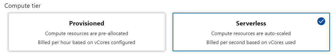
Now we have one more option: Azure SQL Database Serverless. It’s not a product, but a pricing tier of Azure SQL Databases, although it offers slightly different features. 

The best way to understand this new pricing tier is comparing it with the database option “auto close”: When no connection is active on the database, the database shuts down and stop charging our azure account. When the following connection request arrives, the database will start again, making the connection slower than the rest, but only the connection, all further requests will be regular. It’s cheaper, of course, since we are only charged by the time the database is in use, this makes this tier cheaper than the usual Azure SQL Database, but the “auto-close” behaviour maybe not good for some environments.

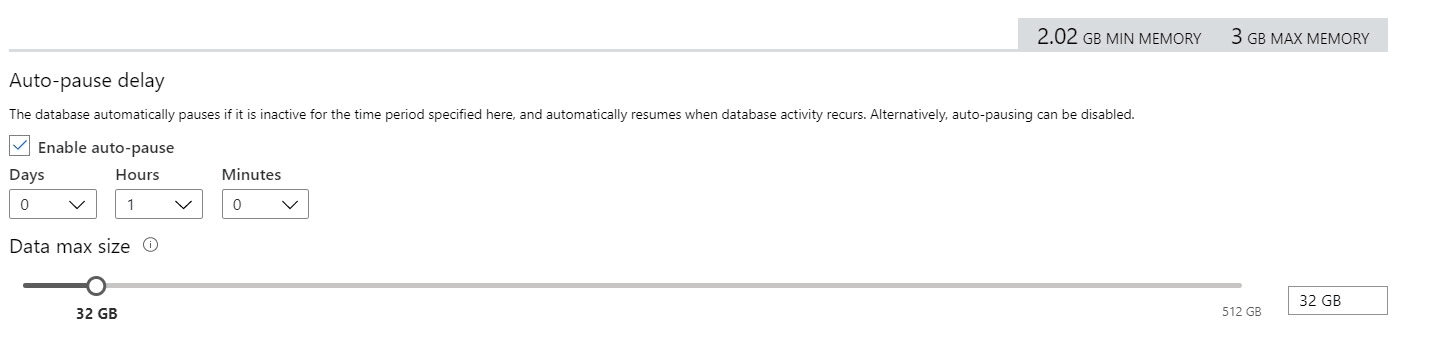
Serverless databases have an additional configuration called Auto-Close Delay. You can define after how long time of inactivity the database should shut down. The minimum amount of time is 1 hour. This configuration can prevent disruptions during work hours. If we find the correct delay configuration the database may shut down only out of working hours.

In the future, a new feature to allow us to automate the start and shutdown may appear, providing us with better control and more savings.

More about Azure SQL Database Serverless: https://docs.microsoft.com/en-us/azure/sql-database/sql-database-serverless

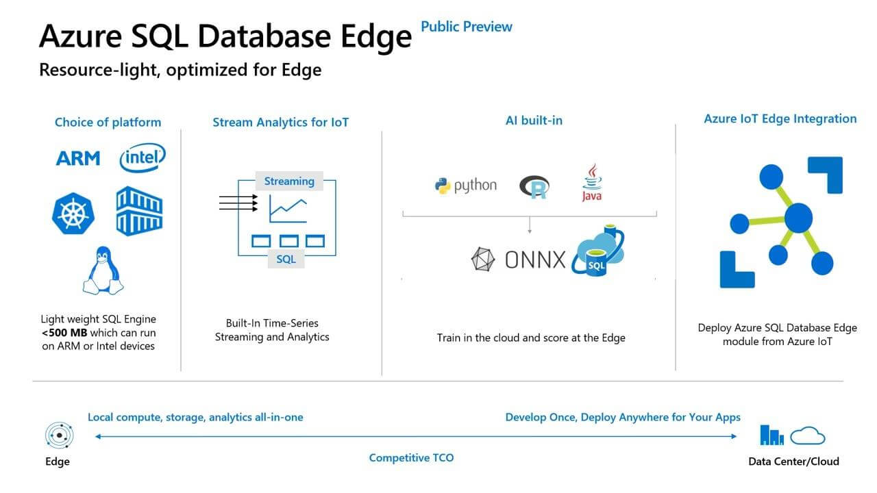
SQL Database Edge

IOT devices, especially in industries, send constant information to servers in order to the server monitor the device and discover if there is something wrong. More than just monitor after the device failure, the servers can run machine learning models over the data to identify potential future failures according to the device’s history.

The weakness of this architecture is the need of the devices to send the data to the server in order to be analysed and only then the server will be able to take an action, maybe changing some device configuration, or sending some alert.

SQL Database Edge is intended exactly to solve this weakness. It’s a SQL Server Edition which can be installed inside the IOT device. Instead of sending the data to the server, the IoT device can save the data in SQL Database Edge and execute the machine learning models using SQL Server, which has the SQL Server Machine Learning Service. In this way, the own device can identify possible future failures and take the possible actions to work around it or send an alert.

Empowering the device, we distribute the load from the server to hundreds or thousands of devices, allowing for faster and more reliable problem identification and workaround using machine learning models.

One more interesting detail is the ability to distribute Azure SQL Database Edge to the devices using IOT Hub.

You can read more about Azure SQL Database Edge here: https://azure.microsoft.com/en-us/services/sql-database-edge/

Learn more about SQL Server Machine Learning Service on this link: https://docs.microsoft.com/en-us/sql/advanced-analytics/what-is-sql-server-machine-learning?view=sql-server-ver15

More about IOT Hub on this link: https://azure.microsoft.com/en-us/services/iot-hub/

Accelerate Data Recovery

This is a new SQL Server 2019 feature which is being much highlighted, not only in PASS Summit.

Long-running operations are something very common to happen. However, sometimes, after 1 or 2 hours of a running operation, some junior DBA may decide it was too much and try to kill the process and rollback. Here the problem begins.

In order to stop the running transaction, all the activities need to be rolled back and this can take almost or even the same time the transaction has taken until the kill was requested. There is no solution, the DBA can only wait for the rollback.

The Accelerated Data Recovery (ADR) arrived with Hyperscale cloud database, announced in PASS Summit 2018. This year, ADR was included in SQL Server 2019. It allows for a fast recovery, without all the rollback waiting time that usually happens.

ADR uses row versioning techniques, but with a different internal structure than the one used by snapshot isolation level.

 

In order to know more about ADR, check these links: 

https://www.linkedin.com/pulse/sql-server-2019-how-saved-world-from-long-recovery-bob-ward/

https://www.red-gate.com/simple-talk/sql/database-administration/how-does-accelerated-database-recovery-work/

Azure ARC

Microsoft knows many companies use more than a single cloud provider. If Microsoft relies only on their cloud services, the war among cloud providers would be difficult, Microsoft can win some, lose others. So, why not a complete change in the battlefield?

Azure ARC allows the deployment and management of Microsoft cloud services to many different clouds: Azure, Google, AWS, all the deployment and management made from a single tool – Azure ARC. This completely changes the battlefield, even if one company has some reason to use a different cloud provider, they can still use Azure ARC to manage the entire environment and even deploy Microsoft services to other cloud providers.

Even more: Azure ARC also allows the deployment of Azure Services to on-premises services.

During the demonstration, Azure ARC was able to provision an Azure SQL Managed Instance in 30 seconds. It was incredible! Just a few weeks before I have talked about Azure SQL Managed Instance and the provisioning time was 3 hours or more. So, I asked at the Data Clinic, how was it possible? How could Azure ARC cause a so huge difference in the provision time?

The answer was very interesting: Because Azure ARC was provisioning the managed instance inside a container. In this case, would the container version of a SQL Managed Instance have any difference in relation to the regular version of a SQL Managed Instance? Yes, they will be slightly different, but the difference is not clearly documented yet.

In order to learn more about Azure Arc you can access this link: https://azure.microsoft.com/en-us/services/azure-arc/

Azure Synapse Analytics

It’s an oversimplification think that Azure Synapse Analytics is a new name for Azure SQL Datawarehouse. Azure Synapse Analytics contains Azure SQL Datawarehouse, but also contains many new features. It seems that it’s going to be a central point for all, or almost all, Azure Data Platform.

One very important new feature is the Azure Synapse Studio. This new tool creates a unified experience among many data platform services: Azure SQL Datawarehouse, Spark, Power BI and more being used from a single front-end tool.

Explaining in a better way: from the Azure Synapse Studio we have access to the Data Warehouse model in Azure SQL Datawarehouse (this name will die, now it’s Azure Synapse Analytics), manipulation of the data using Spark (I’m not sure if it’s linked with Databricks), machine learning models with Azure Machine Learning and visualization dashboards with Power BI, this one connected to the Power BI portal. You can see the changes made in the portal and anything you change from Synapse Analytics will affect the portal.

Can you make any kind of Power BI implementation inside Azure Synapse Studio, such as dataflows and so on? Not yet, but it’s just a beginning, it’s expected to evolve a lot.

In summary, Azure Synapse Analytics is much more than only Azure SQL Datawarehouse, it’s not a only a name change.

You can learn more about Azure Synapse Analytics on these links:

https://azure.microsoft.com/en-us/blog/simply-unmatched-truly-limitless-announcing-azure-synapse-analytics/

https://azure.microsoft.com/en-us/services/synapse-analytics/

Data Tools for Synapse Analytics

SQL Server Data Tools – SSDT – is around for many years, even more than Entity Framework Migrations, which is broadly used today.

I have used SQL Server Data Tools as part of the deployment process in many projects, it’s great to control the version of the database and make schema compares.

The most recent versions were a bit disappointing, the features for schema compare were reduced, I never discovered why. Due to that, the best recommendation was to go for 3^rd part tools when needed.

It seems our relationship with SSDT is getting into a new chapter. SSDT has a new database project for Synapse Analytics, allowing us to create our data warehouse structure in SSDT and control the CICD process.

You can learn more about SSDT and Synapse Analytics on this link: https://cloudblogs.microsoft.com/sqlserver/2019/11/07/new-in-azure-synapse-analytics-cicd-for-sql-analytics-using-sql-server-data-tools/

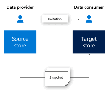
Azure Data Share

Data Share is a new azure service which allows a company to share data with other companies.

Is it better than creating services for the other company?

Well, using Data Share we are manipulating data, sharing parts of our data lake without need to develop something. In the same way, the other company will receive data in order to input in their own system. Is this a benefit? Maybe.

Another possible reason to use Data Share would be for governance: all shared pieces of data would be controlled in the same place, the data shares. However, it may only work well among companies using Azure, if the other company is using another cloud service, I believe data share may not work.

You can read more about Data share on this link: https://docs.microsoft.com/en-us/azure/data-share/

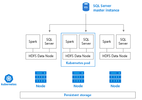
Big Data Cluster

Big Data Clusters are the most highlighted feature in SQL Server 2019. A big summary of what it is would be saying it’s a Microsoft implementation of a Hadoop and Data Lake solution.

Would you like to know more about Hadoop? Check this link: https://hadoop.apache.org/

Learn more about Data Lake on this link: https://en.wikipedia.org/wiki/Data_lake

Let’s simplify the explanation, step by step. Big Data Cluster is an implementation of a Cluster processing solution. This means this feature allows to create a set of servers, with a master node and slave nodes. The master node can receive jobs to process, break these jobs among the slave nodes and collect the results later, resulting the job being processed by many servers as a set, allowing SQL Server to process huge amounts of data.

In the past, this solution was built before using the name of Parallel Data Warehouse. PDW is a SQL Server appliance, but it can be easily understood as a different SQL Server edition. It’s a cluster for parallel processing, exactly as Big Data Cluster. What’s the difference?

You can learn more about Parallel Data Warehouse on this link: https://docs.microsoft.com/en-us/sql/analytics-platform-system/parallel-data-warehouse-overview?view=aps-pdw-2016-au7

The difference is in relation to the language and storage of the data. PDW is totally based on SQL architecture and language. On the other hand, we have for a long time an open architecture called Hadoop and some variations of it, such as Spark.

During the growth of Azure and the cloud environment, both solutions were created in the cloud. PDW was created as SQL Data Warehouse while Hadoop was created as HD Insight, which provides many flavours of Hadoop, such as Spark and more. It became a kind of a race to see which technology would conquer the heart of the market, parallel processing clusters based in SQL or based in Hadoop.

Learn more about HD Insight on this link: https://azure.microsoft.com/en-us/services/hdinsight/

Big Data Cluster is a Hadoop-like solution which can be used in the on-premises environment. However, it’s way more than a simple Hadoop-like solution. Big Data clusters use HDFS Tiering to create Data Virtualization and allow us the creation of a Data Lake, an environment where the data doesn’t need to be moved from its source location in order to be processed.

HDFS tiering was also introduced to us during a sponsored breakfast organized by DELL. It’s a feature linked to Big Data Cluster in SQL Server 2019 which allow us to mount external storages into a single HDFS storage. This leads us to the Data Lake concept: instead of moving the data among storages and technologies, leave the data in its place and process the data where it already is.

You can read more about HDFS tiering here: https://docs.microsoft.com/en-us/sql/big-data-cluster/hdfs-tiering?view=sql-server-ver15

Learn more about Data Virtualization on this link: https://blogs.technet.microsoft.com/machinelearning/2017/06/21/data-virtualization-unlocking-data-for-ai-and-machine-learning/

Another huge difference is the use of Polybase. In order to reach the data sources, Big Data Cluster uses Polybase. However, that’s not the old Polybase we discovered in SQL Server 2016. That’s a new Polybase with support to many different data sources, such as Oracle and much more. Polybase uses its pushdown technology to delegate the processing of SQL predicates to the remote machine responsible for the data.

I still have a lot to understand and write about the evolution of Polybase, because the old Polybase in SQL Server 2016 required a server configuration to set the technology to which the connection would be made, so one SQL Server instance would be tied with a single technology source for Polybase. Besides that, the pushdown technology was very difficult to configure with Hadoop. I believe all these have changed, resulting in the Big Data Clusters, an on-premise (or IaaS) solution for the creation of a Data Lake.

Learn more about Polybase on this link: https://docs.microsoft.com/en-us/sql/relational-databases/polybase/polybase-guide?view=sql-server-ver15

You can read more about Big Data Clusters on this link: https://docs.microsoft.com/en-us/sql/big-data-cluster/big-data-cluster-overview?view=sql-server-ver15

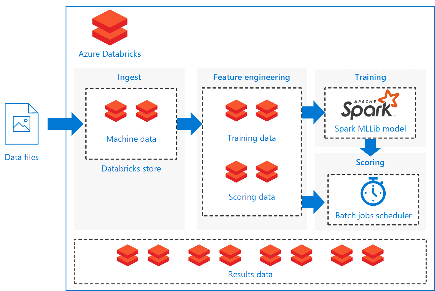
Azure Databricks

Databricks is Spark with a new name. This was everything I knew about Databricks before the PASS Summit and this leaves a lot of questions.

Since we already had Spark working as one of the flavours of HDInsight, why we need Databricks?

I got two answers for that:

A) Databricks is a more complete spark, since it loads a more complete set of modules by default than the Spark we can provision with HDInsight.

B) Databricks doesn’t have the provision problem. Spark in HDInsight needs to be provisioned, used and deleted because the cost to have the Spark servers provisioned is huge. Databricks, on the other hand, doesn’t have this problem, it charges you for the time you use it.

You can learn about this provisioning challenge on this link: https://docs.microsoft.com/en-us/azure/data-factory/v1/data-factory-compute-linked-services#azure-hdinsight-on-demand-linked-service

I loved the second explanation, and this leads us to the next question. However, I would find later this was an incomplete answer. The correct answer, but incomplete.

Since Databricks doesn’t have the provisioning problem anymore, it’s competing with Azure Data Lake, isn’t it? Aren’t both doing the same thing?

The unofficial answer I received was: Yes, they are. However, Azure Data Lake its language, U- SQL, are dead, you shouldn’t build anything new with them

First, it’s important for you to mind that in this context I’m not talking about Data Lake Storage, which is alive and kicking. I’m talking about Azure Data Lake and its language, U-SQL, which were a cluster processing solution on-demand, without the provisioning challenges. At some point, Azure Data Lake started to be called Azure Data Lake Analytics.

You can read more about Azure Data Lake Analytics here: https://azure.microsoft.com/en-us/services/data-lake-analytics/

Learn more about U-SQL language on this link: https://docs.microsoft.com/en-us/u-sql/

Another thing you should mind is that this is an unofficial answer. If you will consider this or not, it’s your choice, according how usually unofficial answers from people close to Microsoft are proven to be true sometime later.

These are not the only advantages of Databricks. The demonstrations during the sessions highlighted how Databricks keeps a record of machine learning training models in such a way we can identify a history of improvement according we work in our ML models.

It’s not clear how much would this be linked to Azure Machine Learning, but it doesn’t seem to be a kind of link such as Synapse Analytics has with Power BI.

Databricks also has an improved storage which received its own name: Delta Lake.

You can read more about Databricks on this link: https://azure.microsoft.com/en-us/services/databricks/

Learn more about Delta Lake on this link: https://docs.microsoft.com/en-us/azure/databricks/delta/delta-intro

Get more information about Azure Machine Learning: https://docs.microsoft.com/en-us/azure/machine-learning/overview-what-is-azure-ml

Power BI

One of the main highlights for Power BI was the Data Protection and Governance new features. This show how Microsoft is engaged in turning Power BI into an enterprise product.

In summary, Power BI will have a link with Sensitive Labels already used in Microsoft Office in order to classify information. Users will be able to classify the information as confidential and other levels and this new feature comes with additional features for monitoring, permissions, governance and so on.

You can learn more about Sensitive Labels on this link: https://docs.microsoft.com/en-us/microsoft-365/compliance/sensitivity-labels

Well, I’m not so sure if this will become something usual, Sensitive Labels require an additional level of management and planning in the organization, I don’t see many clients using this feature.

You can read more about these features here: https://powerbi.microsoft.com/en-us/blog/announcing-new-data-protection-capabilities-in-power-bi/

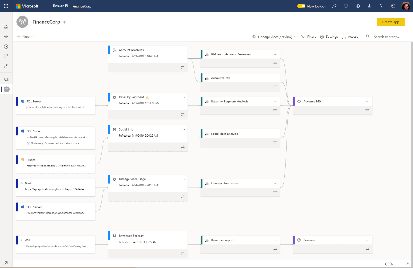
In some ways linked to this, but way more important is the Data Lineage feature, an important feature for data warehouse environments.

In the past, Microsoft tried to include this feature inside ETL tools, it was when SSIS was still called DTS (ops, this may reveal my age!). It didn’t get the attention it deserves, in my opinion not because the feature was bad, but because usually data lineage, although very important, is way down in the list of concerns when building a data warehouse and many people working on this don’t even know exactly what data lineage is and why it’s important.

As the name stands for, the Data Lineage feature keeps track of the source data used to produce a report or dashboard. This feature can save your job when, after building a very expensive data warehouse, two dashboards built by different users show opposite information about the company business. Using the Data Lineage, you can track the information used by the users and identify why the dashboards are different, understanding each dashboard point of view.

So, will this feature work this time? I hope so.

More about Power BI Data Lineage: https://docs.microsoft.com/en-us/power-bi/service-data-lineage

Now, let’s talk about the most surprising news about Power BI: the fact Microsoft is moving Power BI towards a position to replace Azure Analysis Service. Yes, replace Azure Analysis Services.

In order to better understand this, let’s go back in time. SQL Server Analysis Services (SSAS) is an on-premises server built to create Semantic Models as Data Marts.

Data Mart is a focused piece of the Data Warehouse which can be distributed through the company. That’s why Data Marts are usually built as Semantic Models, a model which can be easily understood by business people, less complex than the entire Data Warehouse

On this link, you will find more information about this move: https://powerbi.microsoft.com/en-us/blog/power-bi-premium-and-azure-analysis-services/

Before mentioning the most surprising news about Power BI, let’s analyse the current relationship between SSAS and Power BI.

SSAS is a tool which allows us to create a semantic model for our Data Warehouse. According to the data warehouse architecture, this is a Data Mart, a focused piece of the entire DW. The SSAS data mart is not only focused, but it’s a semantic model, meaning it’s built to be self-explaining to businesspeople. One of the best client tools for SSAS is Excel, once connected to SSAS, the data mart is exposed as a cube, allowing the business user to create pivot table reports using the measures they need at the moment, in a tool they are already used to.

SSAS supports two types of models: Multi-dimensional and Tabular. They have many differences between them, but these differences are disappearing with the evolution of the tool, although we can’t say yet they have the same features.

In order to better understand the difference between the two models, you can follow the two articles in which I illustrate how to build the same data mart with each of the models, highlighting the differences.

Multi-dimensional model: https://www.red-gate.com/simple-talk/sql/bi/creating-a-date-dimension-in-an-analysis-services-ssas-cube/

Tabular model: https://www.red-gate.com/simple-talk/sql/bi/creating-a-date-dimension-in-a-tabular-model/

You can learn more about SSAS semantic model on this link: https://blogs.msdn.microsoft.com/microsoft_press/2017/10/23/designing-a-multidimensional-bi-semantic-model/

Azure Analysis Services only implements the tabular model, not the multi-dimensional model. This creates questions about the future of the multi-dimensional model, although the differences/limitations of the tabular in relation to the multi-dimensional. For example, I’m not a fan of the tabular limitation to have only one active relationship between two tables. What do you think about? Let’s talk more in the comments.

Power BI, on the other hand, was created to be a Visualization and Self-Service BI tool. The idea is to allow the business users to access the corporate Data Warehouse/Data Mart and merge it with any additional information the business needs, even information collected from the web. In this way, the user doesn’t need to make special requests to the corporate IT department, avoiding delays and overwhelming the IT department. As part of the Self-Service BI concept, Power BI also offers Self-Service ETL using Power Query and, more recently, Power BI Dataflows, allowing even a business user to create ETL code to retrieve the needed information.

Power BI was born from Excel plug-ins. Each part of Power BI was a different Excel plug-in, such as Power Query and Power Pivot. Power Pivot, on the other hand, was created from the same tabular engine than SSAS, just with some additional size limitations to fit into Excel.

Therefore, Power BI, SSAS and Azure Analysis Services share the same core engine for the tabular model and Microsoft is working to eliminate the differences. It makes sense the idea of replacing Azure Analysis Services with Power BI, leaving only two questions without a clear answer:

1. The complete set of tabular model features is only available in Power BI Premium, which is expensive. Power BI Pro has limitations which prevent the development of a complete tabular semantic model. Analysis Services, on the other hand, has SSAS as an on-premises option, allowing the company to start the development on the correct way and scale up for bigger and cloud editions in the future. How to solve this dilemma?
2. Will the tabular model, an in-memory solution, really replace the multi-dimensional model, which could store pre-calculations of many combinations of the dimensions?

On this link, you will find more information about the replacement move between power bi premium and Azure Analysis Services: https://powerbi.microsoft.com/en-us/blog/power-bi-premium-and-azure-analysis-services/

 

Conclusion

2020 is starting full of new and exciting technologies for Data Platform in the cloud, it’s time to recycle our knowledge.

 

The post Microsoft Data Platform 2020 appeared first on Simple Talk.

from Simple Talk https://ift.tt/3dEHecA
via

Reduce CPU of Large Analytic Queries Without Changing Code

When Microsoft came out with columnstore in SQL Server 2012, they introduced a new way to process data called Batch Mode. Batch mode processes a group of rows together as a batch, instead of processing the data row by row. By processing data in batches, SQL Server uses less CPU than row by row processing. To take advantage of batch mode, a query had to reference a table that contained a column store index. If your query only involved tables that contain data in row stores, then your query would not use batch mode. That has now changed. With the introduction of version 15.x of SQL Server, aka SQL Server 2019, Microsoft introduced a new feature call Batch Mode on Rowstore.

Batch Mode on Rowstore is one of many new features that was introduced in the Azure SQL Database and SQL Server 2019 to help speed up rowstore queries that don’t involve a column store. The new Batch Mode on Rowstore feature can improve performance of large analytic queries that scan many rows, where these queries aggregate, sort or group selected rows. Microsoft included this new batch mode feature in the Intelligent Query Processing (IQP). See Figure 1 for a diagram from Microsoft’s documentation that shows all the IQP features introduced in Azure SQL Database and SQL Server 2019. It also shows the features that originally were part of Adaptive Query Processing included in the older generation of Azure SQL Database and SQL Server 2017.

Figure 1: Intelligent Query Processing

Batch Mode on Rowstore can help speed up your big data analytic queries but might not kick in for smaller OLTP queries (more on this later). Batch mode has been around for a while and supports columnstore operators, but it wasn’t until SQL Server version 15.x that batch mode worked on Rowstores without performing a hack. Before seeing the new Batch Mode on Rowstore feature in action, let me first explain how batch mode processing works.

How Batch Mode Processing Works

When the database engine processes a transact SQL statement, the underlying data is processed by one or more operators. These operators can process the data using two different modes: Row or Batch. At a high level, row mode can be thought of as processing rows of data, one row at a time. Whereas, batch mode processes multiple rows of data together in a batch. The processing of batches of rows at a time versus row by row can reduce CPU usage.

When batch mode is used for rowstore data, the rows of data are scanned and loaded into a vector storage structure, known as a batch. Each batch is a 64K internal storage structure. This storage structure can contain between 64 and 900 rows of data, depending on the number of columns involved in the query. Each column used by the query is stored in a continuous column vector of fixed size elements, where the qualifying rows vector indicates which rows are still logically part of the batch (see Figure 2 which came from a Microsoft Research paper).

Rows of data can be processed very efficiently when an operation uses batch mode, as compared to row mode processing. For instance, when a batch mode filter operation needs to qualify rows that meet a given column filter criteria, all that is needed is to scan the vector that contains the filtered column and mark the row appropriately in the qualifying rows vector, based on whether or not the column value meets the filter criteria.

 

Figure 2: A row batch is stored column-wise and contains one vector for each column plus a bit vector indicating qualifying rows

SQL Server executes fewer instructions per row when using batch mode over row mode. By reducing the number of instructions when using batch mode, queries typically use less CPU than row mode queries. Therefore, if a system is CPU bound, then batch mode might help reduce the environment’s CPU footprint.

In a given execution plan, SQL Server might use both batch and row mode operators, because not all operators can process data in batch mode. When mixed-mode operations are needed, SQL Server needs to transition between batch mode and row mode processing. This transition comes at a cost. Therefore, SQL Server tries to minimize the number of transitions to help optimize the processing of mixed-mode execution plans.

For the engine to consider batch mode for a rowstore, the database compatibility level must be set to 150. With the compatibility level set to 150, the database engine performs a few heuristic checks to make sure the query qualifies to use batch mode. One of the checks is to make sure the rowstore contains a significate number of rows. Currently, it appears that the magic number seems to be 131,072. Dmitry Pilugin wrote an excellent post on this magic number. I also verified that this is still the magic number for the RTM release of SQL Server 2019. That means that batch mode doesn’t kick in for smaller tables (less than 131,072 rows), even if the database is set to compatibility mode 150. Another heuristic check verifies that the rowstore is using either a b-tree or heap for its storage structure. Batch mode doesn’t kick in if the table is an in-memory table. The cost of the plan is also considered. If the database optimizer finds a cheaper plan that doesn’t use Batch Mode on Rowstore, then the cheaper plan is used.

To see how this new batch mode feature works on a rowstore, I set up a test that ran a couple of different aggregate queries against the WideWorldImportersDW database.

Batch Mode on Rowstore In Action

This section demonstrates running a simple test aggregate query to summarize a couple of columns of a table that uses heap storage. The example runs the test aggregate query twice. The first execution uses compatibility level 140, so the query must use row mode operators to process the test query. The second execution runs under compatibility mode 150 to demonstrate how batch mode improves the query processing for the same test query.

After running the test query, I’ll explain how the graphical execution plans show the different operators used between the two test query executions. I’ll also compare the CPU and Elapsed time used between the two queries to identify the performance improvement using batch mode processing versus row mode processing. Before showing my testing results, I’ll first explain how I set up my testing environment.

Setting up Testing Environment

I used the WideWorldImportersDW database as a starting point for my test data. To follow along, you can download the database backup for this DB here. I restored the database to an instance of SQL Server 2019 RTM running on my laptop. Since the Fact.[Order] table in this database isn’t that big, I ran the code in Listing 1 to create a bigger fact table named Fact.OrderBig. The test query aggregates data using this newly created fact table.

Listing 1: Code to create the test table Fact.OrderBig

USE WideWorldImportersDW;
GO
CREATE TABLE Fact.[OrderBig](
        [Order Key] [bigint],
        [City Key] [int] NOT NULL,
        [Customer Key] [int] NOT NULL,
        [Stock Item Key] [int] NOT NULL,
        [Order Date Key] [date] NOT NULL,
        [Picked Date Key] [date] NULL,
        [Salesperson Key] [int] NOT NULL,
        [Picker Key] [int] NULL,
        [WWI Order ID] [int] NOT NULL,
        [WWI Backorder ID] [int] NULL,
        [Description] [nvarchar](100) NOT NULL,
        [Package] [nvarchar](50) NOT NULL,
        [Quantity] [int] NOT NULL,
        [Unit Price] [decimal](18, 2) NOT NULL,
        [Tax Rate] [decimal](18, 3) NOT NULL,
        [Total Excluding Tax] [decimal](18, 2) NOT NULL,
        [Tax Amount] [decimal](18, 2) NOT NULL,
        [Total Including Tax] [decimal](18, 2) NOT NULL,
        [Lineage Key] [int] NOT NULL);
GO
INSERT INTO Fact.OrderBig
   SELECT * FROM Fact.[Order];
GO 100

The code in Listing 1 created the Fact.OrderBig table that is 100 times the size of the original Fact.[Order] table with 23,141,200 rows.

Comparison Test Script

To do a comparison test between batch mode and row mode, I ran two different test queries found in Listing 2.

Listing 2: Test script

USE WideWorldImportersDW;
GO
-- Turn on time statistics
SET STATISTICS IO, TIME ON;
-- Clean buffers so cold start performed 
DBCC DROPCLEANBUFFERS
GO
-- Prepare Database Compatibility level for Test #1 
ALTER DATABASE WideWorldImportersDW SET COMPATIBILITY_LEVEL = 140;
GO
-- Test #1
SELECT [Customer Key], 
       SUM(Quantity) AS TotalQty,
       AVG(Quantity) AS AvgQty, 
       AVG([Unit Price]) AS AvgUnitPrice
FROM Fact.[OrderBig]
WHERE [Customer Key] > 10 and [Customer Key] < 100
GROUP BY [Customer Key]
ORDER BY [Customer Key];
GO
-- Clean buffers so cold start performed
DBCC DROPCLEANBUFFERS
GO
-- Prepare Database Compatibility level for Test #2
ALTER DATABASE WideWorldImportersDW SET COMPATIBILITY_LEVEL = 150;
GO
-- Test #2
SELECT [Customer Key], 
     SUM(Quantity) AS TotalQty,
        AVG(Quantity) AS AvgQty, 
        AVG([Unit Price]) AS AvgUnitPrice
FROM Fact.[OrderBig]
WHERE [Customer Key] > 10 and [Customer Key] < 100
GROUP BY [Customer Key]
ORDER BY [Customer Key];
GO

The code in Listing 2 executes two different tests, collects some performance statistics, and cleans the data buffer cache between each test. Both tests run the same simple aggregate query against the Fact.OrderBig table. Test #1 runs the aggregate SELECT statement using compatibility level 140, whereas Test #2 runs the same aggregate SELECT statement using compatibility level 150. By setting the compatibility level to 140, Test #1 uses row mode processing. Whereas Test #2, uses compatibility level 150, so batch mode can be considered for the test query. Additionally, I turned on the TIME statistics so I could measure performance (CPU and Elapsed time) between each test. By doing this, I can validate the performance note in Figure 3, that was found in this Microsoft documentation.

Figure 3: Documentation Note on Performance

When I ran my test script in Listing 2, I executed it from a SQL Server Management Studio (SSMS) query window. In that query window, I enabled the Include Actual Execution Plan option so that I could compare the execution plans created for both of my tests. Let me review the execution artifacts created when I ran my test script in Listing 2.

Review Execution Artifacts

When I ran my test script, I collected CPU and Elapsed Time statistics as well as the actual execution plans for each execution of my test aggregate query. In this section, I’ll review the different execution artifacts to compare the differences between row mode and batch mode processing.

The CPU and Elapsed time statistics, as well as the actual execution plan for when I ran my first test query, which was using compatibility level 140, can be found in Figure 4 and Figure 5 respectfully.

Figure 4: CPU and Elapsed Time Statistics for Test #1

Figure 5: Actual Execution Plan under Compatibility Level 140 for Query 1

Figure 6 and 7 below, show the time statistics and the actual execution plan when I ran my test query under compatibility level 150.

Figure 6: Execution Statistics for Test #2

Figure 7: Execution Plan for Test #2

The first thing to note is that the plan that ran under compatibility level 150 (Figure 7) is more streamlined than the one that ran under compatibility mode 140 (Figure 6). From just looking at the execution plan for the second test query, I can’t tell whether or not the query (which ran under compatibility mode 150) uses batch mode or not. To find out, you must right-click on the SELECT icon in the execution for the Test #2 query (Figure 7) and then select the Properties item from the context menu. Figure 8 shows the properties of this query.

Figure 8: Properties for Compatibility Level 150 Query (Test #2)

Notice that the property BatchModeOnRowstoreUsed is True. This property is a new showplan attribute that Microsoft added in SSMS version 18. When this property is true, it means that some of the operators used in processing Test #2 did use a batch mode operation on the Rowstore Fact.OrderBig table.

To review which operators used Batch Mode on Rowstore, you must review the properties of each operator. Figure 9 has some added annotations to the execution plan that shows which operators used batch mode processing and which ones used row mode processing.

Figure 9: Execution Plan for Batch Mode query with Operator property annotations

If you look at the Table Scan (Heap) operator, you can see that the Fact.OrderBig table is a RowStore by reviewing the Storage Property. You can also see that this operation used batch mode by looking at the Actual Execution Mode property. All the other operators ran in batch mode, except the Parallelism operator, which used row mode.

The test table (Fact.OrderBig) contains 23,141,200 rows and the test query referenced 3 different columns. The query didn’t need all those rows because it was filtered to include the rows where the customerid was greater than 10 and less than 100. To determine the number of batches the query created, look at the properties of the table scan operator in the execution plan, which is shown in Figure 10.

Figure 10: Number of batches used for Test #2.

The Actual Number of Batches property in Figure 8 shows that the table scan operator of the test #2 query created 3,587 batches. To determine the number of rows in each batch, use the following formula: Actual Number of Rows divided by the Actual Number of Batches. By using this formula, I got, on average, 899.02 rows per batch.

The cost estimate for each of the queries is the same, 50%. Therefore, to measure performance between batch mode and row mode, I’ll have to look at the TIME statistics.

Comparing Performance of Batch Mode and Row Mode

To compare performance between running batch mode and row mode queries, I ran my test script in Listing 2 ten different times. I then averaged the CPU and Elapsed times between my two different tests and then graphed the results in the chart found in Figure 11.

Figure 11: CPU and Elapsed time Comparison between Row Mode and Batch Mode

The chart in Figure 11 shows that the row mode test query used a little more than 30% more CPU over the batch mode test query. Both the batch and row mode queries ran about the same elapsed time. Just like the note (Figure 4) above suggested, this first test showed considerable CPU improvement could be gained when a simple aggregate query uses Batch Mode processing. But not all queries are created equal when it comes to performance improvements using Batch Mode versus Row Mode.

Not All Queries are Created Equal When It Comes to Performance

The previous test showed a 30% improvement in CPU but little improvement in Elapsed Time. The resource (CPU and Elapsed Time) improvements using Batch Mode operations versus Row mode depend on the query. Here is another contrived test that shows some drastic improvements in Elapsed Time, using the new Batch Mode on Rowstore feature. The test script I used for my second performance test can be found in Listing 3.

Listing 3: Stock Item Key Query Test Script

-- Turn on time statistics
SET STATISTICS IO, TIME ON; 
-- Clean buffers so cold start performed 
DBCC DROPCLEANBUFFERS
GO
-- Prepare Database Compatibility level for Test #1 
ALTER DATABASE WideWorldImportersDW SET COMPATIBILITY_LEVEL = 140;
GO
SELECT [Stock Item Key],[City Key],[Order Date Key],[Salesperson Key],
    AVG(Quantity) OVER(PARTITION BY [Stock Item Key]) AS StockAvgQty, 
    AVG(Quantity) OVER(PARTITION BY [Stock Item Key],[City Key]) 
        AS StockCityAvgQty,
    AVG(Quantity) OVER(PARTITION BY [Stock Item Key],[City Key],
        [Order Date Key]) AS StockCityDateAvgQty,  
    AVG(Quantity) OVER(PARTITION BY [Stock Item Key],[City Key],
        [Order Date Key],[Salesperson Key]) 
        AS StockCityDateSalespersonAvgQty
FROM Fact.OrderBig
WHERE [Customer Key] > 10 and [Customer Key] < 100
-- Clean buffers so cold start performed 
DBCC DROPCLEANBUFFERS
GO
-- Prepare Database Compatibility level for Test #2 
ALTER DATABASE WideWorldImportersDW SET COMPATIBILITY_LEVEL = 150;
GO
SELECT [Stock Item Key],[City Key],[Order Date Key],[Salesperson Key],
    AVG(Quantity) OVER(PARTITION BY [Stock Item Key]) AS StockAvgQty, 
    AVG(Quantity) OVER(PARTITION BY [Stock Item Key],[City Key]) 
        AS StockCityAvgQty,
    AVG(Quantity) OVER(PARTITION BY [Stock Item Key],[City Key],
        [Order Date Key]) AS StockCityDateAvgQty,  
    AVG(Quantity) OVER(PARTITION BY [Stock Item Key],[City Key],
        [Order Date Key],[Salesperson Key]) 
        AS StockCityDateSalespersonAvgQty
FROM Fact.OrderBig
WHERE [Customer Key] > 10 and [Customer Key] < 100

In Listing 3, I used the OVER clause to create four different aggregations, where each aggregation had a different PARTITION specification. To gather the performance statistics for Listing 3 queries, I ran this script ten different times. Figure 12 shows the numbers for CPU and Elapsed Time numbers graphically.

Figure 12: CPU and Elapsed Time comparison for Window Function Query test

As you can see by creating the different aggregation in Listing 3, I once again saw a big performance improvement in CPU (around 72%). This time, I also got a big improvement in Elapsed Time (a little more than 45%) when batch mode was used. My testing showed that not all queries are created equal when it comes to performance. For this reason, I recommend you test all the queries in your environment to determine how each query performs using this new Batch Mode on Rowstore feature. If you happen to find some queries that perform worse using batch mode, then you can either rewrite the queries to perform better or consider disabling batch mode for those problem queries.

Disabling Batch Mode on Row Store

If you find you have a few queries that don’t benefit from using batch mode, and you don’t want to rewrite them, then you might consider turning off the Batch Mode on Rowstore feature with a query hint.

If you use the DISALLOW_BATCH_MODE hint, you can disable Batch Mode on Rowstore feature for a given query. The code in Listing 4 shows how I disabled batch mode for the first test query I used in this article.

Listing 4: Using “DISALLOW BATCH MODE” hint to disable batch mode for a single query

SELECT [Customer Key], 
       SUM(Quantity) AS TotalQty,
       AVG(Quantity) AS AvgQty, 
       AVG([Unit Price]) AS AvgUnitPrice
FROM Fact.[OrderBig]
WHERE [Customer Key] > 10 and [Customer Key] < 100
GROUP BY [Customer Key]
ORDER BY [Customer Key]
OPTION(USE HINT('DISALLOW_BATCH_MODE'));

When I ran the query in Listing 4 against the WideWorldImportersDW database running in compatibility mode 150, the query didn’t invoke any batch mode operations. I verified this by reviewing the properties of each operator. They all processed using a row mode operation. The value of using the DISALLOW_BATCH_MODE hint is I can disable the batch mode feature for a single query. This means it’s possible to be selective on which queries will not consider batch mode when your database is running under compatibility level 150.

Alternatively, you could disable the Batch Mode on Rowstore feature at the database level, as shown in Listing 5.

Listing 5: Disabling Batch Mode at the database level

-- Disable batch mode on rowstore
ALTER DATABASE SCOPED CONFIGURATION SET BATCH_MODE_ON_ROWSTORE = OFF;

Disabling the batch mode feature at the database level still allows other queries to take advantages of the other new 15.x features. This might be an excellent option to use if you wanted to move to version 15.x of SQL Server while you complete testing of all of your large aggregation queries to see how they are impacted by the batch mode feature. Once testing is complete, reenable batch mode by running the code in Listing 6.

Listing 6: Enabling Batch Mode at the database level

-- Enable batch mode on rowstore
ALTER DATABASE SCOPED CONFIGURATION SET BATCH_MODE_ON_ROWSTORE = ON;

By using the hint or database scoped configure method to disable batch mode, I have control over how I want this new feature to affect the performance of my row mode query operations. It is great that the team at Microsoft allows these different methods to disable/enable the Batch Mode on Rowstore feature. By allowing these different options for enable/disabling batch mode on rowstore, I have more flexibility in how I roll out the batch mode feature across a database.

Which Editions Support Batch Mode?

Before you get too excited about how this feature might help the performance of your large analytic queries, I have to tell you the bad news. Batch Mode on Rowstore is not available to all version of SQL. Like many cool new features that have come out in the past, they are first introduced in Enterprise edition only, and then over time, they might become available in other editions. Batch Mode on Rowstore is no exception. As of the RTM release of SQL Server 2019, the Batch Mode on Rowstore feature is only available in Enterprise Edition, as documented here. Also note that developer edition supports Batch Mode on Rowstore, but of course cannot be used for production work. Be careful when doing performance testing of this new feature on the developer edition of SQL Server 2019 if you plan to roll out your code into any production environment except Enterprise. If you want to reduce your CPU footprint using this new feature, then you better get out your checkbook and upgrade to Enterprise edition, or just wait until Microsoft rolls this feature out to other editions of SQL Server. It also works on Azure SQL Database.

Reduce CPU of Large Analytic Queries Without Changing Code

If you have large analytic queries that perform aggregations, you might find that using the new Batch Mode on Rowstore feature improves CPU and Elapsed time without changing any code if your query environment meets a few requirements. The first requirement is that your query needs to be running using SQL Server version 15.x (SQL Server 2019) or better. The second requirement is you need to be running on an edition of SQL Server that supports the Batch Mode on Rowstore feature. Additionally, the table being queried needs to have at least 131,072 rows and be stored in a b-tree or heap before batch mode is considered for the table.

I am impressed by how much less CPU and Elapsed time was used for my test aggregation queries. If you have a system that runs lots of aggregate queries, then migrating to SQL Server 2019 might be able to eliminate your CPU bottlenecks and get some of your queries to run faster at the same time.

 

 

The post Reduce CPU of Large Analytic Queries Without Changing Code appeared first on Simple Talk.

from Simple Talk https://ift.tt/3dueKSM
via

DevOps is Essential for Analytics

The term DevOps was coined in the early 2000s to improve the speed and resiliency of the delivery of features and applications and providing more value to customers. It’s not about any particular technology, methodology, or toolset, but automation of everything from unit testing to building environments to delivery is part of it. DevOps also means broadly changing the culture in a department or company by breaking down silos between teams. “Well, it worked on my machine” doesn’t fly in a DevOps organization. All teams are responsible for the outcome: quickly bringing value to the customer.

Like any catchy term, there have been others inspired by DevOps. You may see ITOps, NetOps, SecOps and even NoOps. One term that may be confusing is DataOps. At first glance, it sounds like bringing the database into DevOps, but that is not accurate:

“DataOps is an automated, process-oriented methodology, used by analytic and data teams, to improve the quality and reduce the cycle time of data analytics. While DataOps began as a set of best practices, it has now matured to become a new and independent approach to data analytics. DataOps applies to the entire data lifecycle from data preparation to reporting and recognizes the interconnected nature of the data analytics team and information technology operations.”

DataOps involves using agile principles, testing, automation, and measuring outcomes to ensure that valuable information is in the right hands at the right time and brings value to decision-makers more quickly. Quality is improved, and data scientists and analysts have more time to innovate and spend less time on repeatable, manual processes.

While DataOps involves the lifecycle for analytics, including artificial intelligence and machine learning, Database DevOps ensures the proper delivery of changes to the transactional and reporting databases. These databases typically act as the sources of data for analytics. Database DevOps means adding source control for schema changes, using tools to automate the creation of database deployment scripts, and working in cross-functional teams (i.e., DBAs working with developers). Historically, changes to the database have been done manually and have often been a bottleneck to deploying features which depend on new or altered tables and other objects.

The tools used for Database DevOps help database administrators quickly provision sanitized copies of databases that resemble production for development, testing, quality assurance, and staging environments and automate the process as part of the pipeline. The tools help ensure that “quick fixes” and “one-offs” don’t bypass the pipeline so that production and other environments stay in sync. After talking with database administrators in the transition of converting to DevOps, it’s a big change to how they have worked in the past, but the benefits are worth it.

Database DevOps is essential for DataOps. In the end, Database DevOps means accurate and consistent data which is critical for analytics, artificial intelligence, and machine learning.

Commentary Competition

Enjoyed the topic? Have a relevant anecdote? Disagree with the author? Leave your two cents on this post in the comments below, and our favourite response will win a $50 Amazon gift card. The competition closes two weeks from the date of publication, and the winner will be announced in the next Simple Talk newsletter.

 

The post DevOps is Essential for Analytics appeared first on Simple Talk.

from Simple Talk https://ift.tt/2Wwpmus
via

The Staging Phase of Deployment

Staging is a vital part of doing the deployment of any application, particularly a database quickly, efficiently, and with minimum risk. Though vital, it only gets noticed by the wider public when things go horribly wrong.

On 2nd February 1988, Wells Fargo EquityLine customers noticed, on the bottom of a statement, this message

“You owe your soul to the company store. Why not owe your home to Wells Fargo? An equity advantage loan can help you spend what would have been your children’s inheritance.”

A few days later, the company followed this with an apology:

“This message was not a legitimate one. It was developed as part of a test program by a staff member, whose sense of humor was somewhat misplaced, and it was inadvertently inserted in that day’s statement mailing. The message in no way conveys the opinion of Wells Fargo Bank or its employees.

James G. Jones, Executive Vice President, South Bay Service Center”

This mishap was an accident in Staging. It is so easy to do. It could have been worse. In early 1993, a small UK-based company was working with one of the largest UK telecom companies in launching a new ‘gold’ credit card for their wealthier customers. They needed a mailshot. The mailshot application was in Staging and as not all of the addresses were ready, where there was a NULL name, the programmer flippantly inserted the place-holder ‘Rich Bastard’, before leaving the project. Sadly, the mail addresses that the test mailshot went to were from the live data. His successor unwittingly ran the test. The rest of the story is in IT History. The blameless developer running the test, nonetheless, left the profession and became a vet.

Staging rarely causes a problem for the business: far more frequently, it can save the costly repercussions of a failed deployment. Had the UKs TSB (Trustee Saving Bank) engaged in conventional, properly conducted, staging practices in 2018, they’d have saved their reputation and costs of 330 million pounds. Staging allows potential issues and concerns with a new software release to be checked, and the process provides the final decision as to whether a release can go ahead. The fact that this vital process can occasionally itself cause a problem to the business is ironic. Mistakes in Staging can be far-reaching. It requires dogged attention to detail and method.

Staging

It is often said that the Customers of an application will think it is finished when they see a Smoke and Mirrors demo. Developers think it is done when it works on their machine. Testers think it is complete when it passes their tests. It is only in Staging, when a release candidate is tested out in the production environment, can it be said to be ready for release.

The team that conducts the Staging process within an organisation have a special responsibility. If a production application that is core to the organisations business is being tested, the senior management have a responsibility to ensure that the risk of changes to the business is minimised. They usually devolve this responsibility, via the CIO, to the technical team in charge of Staging, and it is highly unusual that management would ignore the recommendations of that team. If the two don’t communicate effectively, things go wrong. In the spectacular case of TSB,  the release was allowed to proceed despite there being 2,000 defects relating to testing at the time the system went live.

Whether you are developing applications or upgrading customised bought-in packages, these must be checked out in Staging. The Staging function has a uniquely broad perspective on a software release, pulling together the many issues of compliance, maintenance, security, usability, resilience and reliability. Staging is designed to resemble a production environment as closely as possible, and it may need to connect to other production services and data feeds. The task involves checking code, builds, and updates to ensure quality under a production-like environment before the application is deployed. Staging needs to be able to share the same configurations of hardware, servers, databases, and caches as the production system

The primary role of a staging environment is to check out all the installation, configuration and migration scripts and procedures before they’re applied to a production environment. This ensures that all major and minor upgrades to a production environment are completed reliably, without errors, and in a minimum of time. It is only in staging that some of the most crucial tests can be done. For example, servers will be run on remote machines, rather than locally (as on a developer’s workstation during dev, or on a single test machine during test), which tests the effects of networking on the system.

Can Staging be Avoided?

I’ve been challenged in the past by accountants on the cost of maintaining a staging environment. The simplest answer is that it is a free by-product of the essential task of proving your disaster-recovery strategy. Even if no significant developments of database applications are being undertaken in an organisation, you still need a staging environment to prove that, in the case of a disaster, you can recover services quickly and effectively, and that an action such as a change in network or storage has no unforeseen repercussions with the systems that you, in operations, have to support in production. You can only prove that you can re-create the entire production environment, its systems and data in a timely manner by actually doing it and repeating it. It makes sense to use this duplicate environment for the final checks for any releases that need to be hosted by the business. Not all the peripheral systems need to be recreated in their entirety if it is possible to ‘mock’ them with a system with exactly the same interface that behaves in exactly the same way. It isn’t ideal, though: The more reality that you can provide in staging the better.

Staging and Security

Before the Cloud blurred the lines, it was the custom in IT that Staging was done entirely by the operational team in the production setting, which meant a separate Ops office or data-centre. This meant that security for Staging was identical to Production. In a retail bank, for example, where I once worked as a database developer, the actual client data would be used. As my introductory stories illustrated, this could lead to highly embarrassing mistakes. However, security was excellent: To get into the data centre where Staging was done, you needed a key fob, and your movements were logged. There was close supervision, video surveillance, and nobody got a key fob without individual security vetting. It was ops territory, though I was able to call in to check a release because I’d been security-checked. This was a rigorous process that took weeks by a private investigator, an avuncular ex-cop in my case with the eye of a raptor. I explain this to emphasise the point that if the organisation has the security and organisational disciplines, you can use customer data within a production environment for Staging. Without stringent disciplines and supervision, it simply isn’t legally possible. The GDPR makes the responsible curation of personal data into a legal requirement. It doesn’t specify precisely how you do it.

It isn’t likely that you’d want a straightforward copy of the user data, though. Leaving to one side the responsibility that any organisation has for the owners of restricted, personal or sensitive data, it really mustn’t ever contain such data as client email, phone numbers, or messages that are used for messaging, alerts, or push notifications. Any data, such as XML documents of patients’ case histories for example, or anything else that is peripheral in any way to the objectives of Staging, ought to be pseudonymized. The Staging environment is as close as possible to production so that the final checks to the system and the database update scripts for the release are done realistically, but without being on production. As Staging is under the same regime as production, there isn’t a risk to data above that of the production system.

What is In-scope for Staging?

It is difficult to make any hard-and-fast rules about this because so much depends on the size of the organisation, the scale of the application, and the ongoing methodology within IT. Staging is often used to preview new features to a select group of customers or to check the integrations with live versions of external dependencies. Sometimes Staging is suggested as the best place for testing the application under a high load, or for ‘limit’ testing, where the resilience of the production system is tested out. However, there are certain unavoidable restrictions. Once a release enters Staging, there can only be two outcomes: either the release is rejected or goes into production. Staging cannot therefore easily be used for testing for integrity, performance or scalability for that particular release because that requires interaction. It can, of course, feed the information back for the next release, but generally It is much better done in development interactively using standard data sets before release so that any issues can be fixed without halting the staging process. Sometimes there is no alternative If the tests done in Staging show up a problem that is due to the pre-production environment such as data feeds or edge cases within the production data, then the release has to go back to development. Nowadays, where releases are often continuous, Staging can be far more focused on the likely problems of going to production since there are more protections against a serious consequence, by using safety practices such as blue/green, feature toggles, canary or rolling releases

How to Make it Easier for a Deployment in Staging

The most obvious ways of making Staging easy, even in the absence of DevOps, is to involve operations as early as possible in the design and evolution of a development, to tackle configuration and security issues as early as possible, and for the development team to develop techniques for automating as much as possible of the deployment of the application. The ops teams I’ve worked with like the clarity that comes with documentation. Some people find documentation irksome, but documents are the essential lubricant of any human endeavour because they remove elements of doubt, confusion and misunderstanding. As far as development goes, the documentation needs to cover at least the interfaces, dependencies and configuration data. I always include a training manual and a clear statement of the business requirements of the application. Because the Staging team have to judge the ‘maintainability’ of the system, they will want to see the instructions that you provide for the first-line responders to a problem for the production system.

Staging Issues

Several different factors have conspired to make the tasks of the Staging team more complex. These include the demands for continuous integration and rapid deployment. This has made the requirement for automation of at least the configuration management of the Staging environment more immediate. The shift to Cloud-native applications has changed the task of Staging, especially if the architecture is a hybrid one, with components that are hosted, and the presence of legacy systems that contribute data or take data.

As always, there are developments in technology such as the use of containers, perhaps in conjunction with a microservices architecture, that can provide additional challenges. However, these changes generally conspire to force organisations to maintain a permanent staging environment for major applications in active development. If there is a considerable cloud component, this can amplify the charges for cloud services unless ways can be found to do rapid build and tear-down.

Against this rise in the rate of releases and the complexity of the infrastructure, there is the fact that a regularly performed system will usually tend to become more efficient, as more and more opportunities are found for automation and cooperative teamwork.

It is in staging that DevOps processes, and a consistent infrastructure, can help. However, it is crucial to make sure that the specialists who have to check security and compliance have plenty of warning of a release candidate in Staging and are able to do their signoffs quickly. They also may need extra resources and documentation provided for them, so it is a good idea to get these requirements clarified in good time.

An acid test for a manager is to see how long a new team member takes to come up to speed. The faster this happens, the more likely that the documentation, learning materials, monitoring tools, and teamwork are all appropriate. There must be as few mysteries and irreplaceable team members as possible.

Conclusion

Despite the changes in technology and development methodology over the years, the Staging phase of release and deployment is still recognisable because the overall objectives haven’t changed. The most significant change is from big, infrequent releases to small, continuous releases. The problems of compliance have grown, and the many issues of security have ballooned, but the opportunities for automation of configuration management, teamwork and application checks have become much greater. Because releases have a much narrower scope, the checks can be reduced to a manageable size by assessing the risks presented by each release and targeting the checks to the areas of greatest risk. The consequences of a failed release can be minimised by providing techniques such as feature-switching for avoiding rollbacks. However, seasoned ops people will remember with a shudder when a small software update caused a company to lose $400 million in assets in 45 minutes. Staging is important and should never be taken for granted.

 

The post The Staging Phase of Deployment appeared first on Simple Talk.

from Simple Talk https://ift.tt/3b58wqk
via