How to Create an Ubuntu PowerShell Development Environment – Part 3

The series so far:

1. How to Create an Ubuntu PowerShell Development Environment – Part 1
2. How to Create an Ubuntu PowerShell Development Environment – Part 2
3. How to Create an Ubuntu PowerShell Development Environment – Part 3

Over the last few years, Microsoft has made great strides in making their software products available on a wider range of platforms beyond Windows. Many of their products will now run on a variety of Linux distributions (often referred to as “distros”), as well as Apple’s macOS platform. This includes their database product, SQL Server.

One way in which Microsoft achieved cross-platform compatibility is through containers. If you aren’t familiar with containers, you can think of them as a stripped-down virtual machine. Only the components necessary to run the application, in this case, SQL Server, are included. The leading tool to manage containers is called Docker. Docker is an application that will allow you to download, create, start and stop, and run containers. If you want a more detailed explanation of containers, please see the article What is a Container on Docker’s website.

Assumptions

For this article, you should understand the concepts of a container, although no experience is required. See the article from Docker referenced in the previous section if you desire more enlightenment on containers. Additionally, this article assumes you are familiar with the SQL language, as well as some basics of PowerShell. Note that throughout this article, when referencing PowerShell, it’s referring to the PowerShell Core product.

The Platform

The previous articles, How to Create an Ubuntu PowerShell Development Environment Part 1 and Part 2, walked through the steps of creating a virtual machine for Linux development and learning. That VM is the basis for this article. All the code demos in this article were created and run in that specific virtual computer. For best results, you should first follow the steps in that article to create a VM. From there, you will be in a good place to follow along with this article. However, they have been tested on other variations of Ubuntu, CentOS, as well as on macOS.

In those articles, I showed not just the creation of the virtual machine, but the steps to install PowerShell and Visual Studio Code (VSCode), tools you will need in order to complete the demos in this article should you wish to follow along.

For the demo, I am assuming you have download the demo files and opened them in Visual Studio Code within the virtual machine, and are executing individual samples by highlighting the code sample and using the F8 key, or by right-clicking on the selected text and picking run.

The Demo

The code samples in this article are part of a bigger sample I provide on my GitHub site. You’ll find the entire project here. There is a zip file included that contains everything in one easy download, or you can look through GitHub and pick and choose the files you want. GitHub also displays Markdown correctly, so you may find it easier to view the project documentation via GitHub rather than in VSCode.

This article uses two specific files, located in the Demo folder: m11-cool-things-1-docker.ps1 and m11-install-docker.sh. While this article will extract the relevant pieces and explain them, you will find it helpful to review the entire script in order to understand the overall flow of the code.

The Beginning

The first thing the PowerShell script does is use the Set-Location cmdlet to set the current location to the folder where you extracted the demo code. This location should have the Demo, Notes, and Extras folders under it.

Next, make sure Docker is installed, and if not, install it. The command to do this is rather interesting.

bash ./Demo/m11-install-docker.sh

bash is very similar to PowerShell; it is both a terminal and a scripting language. It is native to many Linux distros, including the Ubuntu-based ones. This code uses PowerShell to start a bash session and then executes the bash script m11-install-docker.sh. When the script finishes executing, the bash session ends.

Take a look inside that bash script.

if [ -x "$(command -v docker)" ]; then
    echo "Docker is already installed"
else
    echo "Installing Docker"
    sudo snap install docker
fi

The first line attempts to run a command that will complete successfully if Docker is installed. If so, it simply displays that information to the screen via the echo command.

If Docker is not installed, then the script will attempt to install Docker using the snap utility. Snap is a package manager introduced in the Ubuntu line of distros; other distros use a manager known as flat packs. On macOS, brew is the package manager of choice. This is one part of the demo you may need to alter depending on your distro. See the documentation for your specific Linux install for more details.

Of course, there are other ways to install Docker. The point of these few lines was to demonstrate how easy it is to run bash scripts from inside your PowerShell script.

Pulling Your Image

A Docker image is like an ISO. Just as you would use an ISO image to create a virtual machine, a Docker image file can be used to generate one or more containers. Docker has a vast library of images, built by itself and by many companies, such as Microsoft. These images are available to download and use in your own environments.

For this demo, you are going to pull the image for SQL Server 2017 using the following command.

sudo docker pull mcr.microsoft.com/mssql/server:2017-latest

The sudo command executes the following docker program with administrative privileges. Docker, as stated earlier, is the application which manages the containers. Then you give the instruction to Docker, pull. Pull is the directive to download a container from Docker’s repositories.

The final piece is the image to pull. The first part, mcr.microsoft.com, indicates this image is stored in the Microsoft area of the Docker repositories. As you might guess, mssql indicates the subfolders containing SQL Server images, and server:2017-latest indicates the version of SQL Server to pull, 2017. The -latest indicates this should be the most currently patched version; however, it is possible to specify a specific version.

Once downloaded, it is a good idea to query your local image cache to ensure the download was successful. You can do so using this simple command.

sudo docker image ls

image tells Docker you want to work with images, and ls is a simple listing command, similar to using ls to list files in the bash shell.

Running the Container

Now that the image is in place, you need to create a container to run the SQL Server. Unlike traditional SQL Server configuration, this turns out to be quite simple. The following command is used to not only create the container but run it. Note the backslash at the end of each line is the line continuation character for bash, the interpreter that will run this command (even though you’re in PowerShell). You could also choose to remove the backslashes and just type the command all on one line.

sudo docker run -e 'ACCEPT_EULA=Y' -e 'SA_PASSWORD=passW0rd!' -p 1433:1433 --name arcanesql -d mcr.microsoft.com/mssql/server:2017-latest

The first part of the line starts by passing the run command into Docker, telling it to create and run a new container. In the first -e parameter you are accepting the end user license agreement. In the second -e parameter, you create the SA (system administrator) password. As you can see, I’ve used a rather simple password, you should definitely use something much more secure.

Next, we need to map a port number for the container using the -p parameter. The first port number will be used to listen on the local computer, the second port number is used in the container. SQL Server listens on port 1433 by default, so we’ll use that for both parts of the mapping.

The next parameter, --name, provides the name for the container; here I’m calling it arcanesql.

In the final parameter, -d, you need to indicate what image file should be used to generate the container. As you can see, the command is using the SQL Server image downloaded in the previous step.

You can verify the container is indeed running using the following command.

sudo docker container ls

As with the other commands, the third parameter indicates what type of Docker object to work with, here containers. Like with image, the ls will produce a list of running containers.

Installing the SQL Server Module

Now that SQL Server is up and running, it’s time to start interacting with it from PowerShell Core. First, though, install the PowerShell Core SQL Server module.

Install-Module SqlServer

It won’t hurt to run this if the SQL Server module is already installed. If it is PowerShell will simply provide a warning message to that effect.

If you’ve already installed it, and simply want to make sure it is up to date, you can use the cmdlet to update an already installed module.

Update-Module SqlServer

Do note that normally you would not want to include these in every script you write. You would just need to ensure the computer you are running on has the SQL Server module installed, and that you update it on a regular basis, testing your scripts of course after an update. (For more about testing PowerShell code, see my three-part article on Pester, the PowerShell testing framework, beginning with Introduction to Testing Your PowerShell Code with Pester here on SimpleTalk.)

Running Your First Query

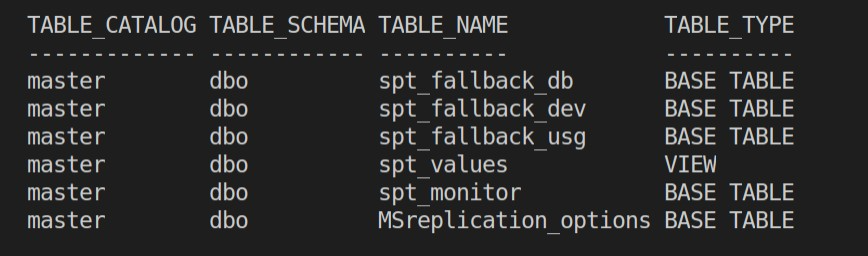
The first query will be very simple; it will return a listing of all tables in the master database so you can see how easy it is to interact with SQL Server and learn the basic set of parameters.

The basic cmdlet to work with SQL Server is Invoke-SqlCmd. It requires a set of parameters, so you’ll place those in variables for easy reference.

$serverName = 'localhost,1433'
$dbName = 'master'
$userName = 'sa'
$pw = 'passW0rd!'
$queryTimeout = 50000
$sql = 'SELECT * FROM master.INFORMATION_SCHEMA.Tables'

For this exercise, you are running the Docker container on the same computer as your PowerShell session, so you can just use localhost for the server name. Obviously, you’ll replace this with the name of your server when working in other environments. Note that you must append the port number after the server name.

Next, you have the database name you’ll be working with, and for this example, it will be master.

The next two parameters are the username and password. In a real-world environment, you’d be setting up real usernames and passwords, but this demo will be simple and just use the SA (system administrator) account built into SQL Server. The password is the same one used when you created and ran the container using the docker run command.

Next up is the query timeout. How long do should PowerShell wait before realizing no one is answering and give up? The timeout is measured in terms of seconds.

The last parameter is the query to run. Here you are running a simple SELECT statement to list the tables in the master database.

Now that the parameters are established in variables, you are ready to call the Invoke-SqlCmd cmdlet to run the query.

Invoke-Sqlcmd -Query $sql `
              -ServerInstance $serverName `
              -Database $dbName `
              -Username $userName `
              -Password $pw `
              -QueryTimeout $queryTimeout

Here you pass in the variables to each named parameter. Note the backtick symbol at the end of each line except the last. This is the line continuation character; it allows you to spread out lengthy commands across multiple lines to make them easier to read.

In the output, you see a list of each table in the master database.

Splatting

As you can see, Invoke-SqlCmd has a fairly lengthy parameter set. It will get tiresome to have to repeat this over and over each time you call Invoke-SqlCmd, especially as the bulk of these will not change between calls.

To handle this, PowerShell includes a technique called splatting. With splatting, you create a hash table, using the names of the parameters for the hash table keys, and the values for each parameter as the hash table values.

$sqlParams = @{ "ServerInstance" = $serverName
                "Database" = $dbName
                "Username" = $userName
                "Password" = $pw
                "QueryTimeout" = $queryTimeout
              }

If you look at the syntax in the previous code example, you’ll see that the key values on the left of the hash table above match the parameter names. For this example, load the values from the variables you created, but you could also have hardcoded the values.

So how do you use splatting when calling a cmdlet? Well, that’s pretty simple. In this next example, you’ll load the $sql variable with a query to create a new database named TeenyTinyDB, and then execute the Invoke-SqlCmd.

$sql = 'CREATE DATABASE TeenyTinyDB'
Invoke-Sqlcmd -Query $sql @sqlParams

Here you call Invoke-SqlCmd, then pass in the query as a named parameter. After that, you pass in the hash table variable sqlParams, but with an important distinction. To make splatting work, you use the @ symbol instead of the normal $ for a variable. When PowerShell sees the @ symbol, it knows to deconstruct the hash table and use the key/values as named parameters and their corresponding values.

There are two things to note. I could have included the $sql as another value in the hash table. It would have looked like “Query” = $sql (or the actual query as a hard-coded value). In the demo, I made them separate to demonstrate that it is possible to mix named parameters with splatting. On a personal note, I also think it makes the code cleaner if the values that change on each call are passed as named parameters and the values that remain fairly static to become part of the splat.

Second, the technique of splatting applies to all cmdlets in PowerShell, not just Invoke-SqlCmd. Feel free to implement this technique in your own projects.

When you execute the command, you don’t get anything in return. On the SQL Server, the new database was created, but because you didn’t request anything back, PowerShell simply returns to the command line.

Creating Tables

For the next task, create a table to store the names and URLs of some favorite YouTube channels. Because you’ll be working with the new TeenyTinyDB instead of master, you will need to update the Database key/value pair in the hash table.

$dbName = 'TeenyTinyDB'
$sqlParams["Database"] = $dbName

Technically I could have assigned the database name without the need for the $dbName variable. However, I often find myself using these values in other places, such as an informational message. Perhaps a Write-Debug “Populating $dbName” message in my code. Placing items like the database name in a variable makes these tasks easy.

With the database value updated, you can now craft a SQL statement to create a table then execute the command by once again using Invoke-SqlCmd.

$sql = @'
CREATE TABLE [dbo].[FavoriteYouTubers]
(
    [FYTID]       INT            NOT NULL PRIMARY KEY
  , [YouTubeName] NVARCHAR(200)  NOT NULL
  , [YouTubeURL]  NVARCHAR(1000) NOT NULL
)
'@
Invoke-Sqlcmd -Query $sql @sqlParams

In this script, you take advantage of PowerShell’s here string capability to spread the create statement over multiple lines. If you are not familiar with here strings, it is the ability to assign a multi-line string to a variable. To start a here string, you declare the variable then make @ followed by a quotation mark, either single quote or double quote, the last thing on the line. Do note it has to be last; you cannot have anything after it such as a comment.

The next one or more lines are what you want the variable to contain. As you can see, here strings make it easy to paste in SQL statements of all types.

To close out a here string, simply put the closing quotation mark followed by the @ sign in the first two positions of a line. This has to be in the first two characters if you attempt to indent the here string won’t work.

With the here string setup, call Invoke-SqlCmd to create the table. As with the previous statement, it doesn’t produce any output, and it simply returns us to the command line.

Loading Data

In this example, create a variable with a SQL query to load multiple rows via an INSERT statement and execute it.

$sql = @'
INSERT INTO [dbo].[FavoriteYouTubers]
  ([FYTID], [YouTubeName], [YouTubeURL])
VALUES
  (1, 'AnnaKatMeow', 'https://www.youtube.com/channel/UCmErtDPkJe3cjPPhOw6wPGw')
, (2, 'AdultsOnlyMinecraft', 'https://www.youtube.com/user/AdultsOnlyMinecraft')
, (3, 'Arcane Training and Consulting', 'https://www.youtube.com/channel/UCTH58i-Gl1bZeATOeC4f25g')
, (4, 'Arcane Tube', 'https://www.youtube.com/channel/UCkR0kwYjQ_gngZ8jE3ki7xw')
, (5, 'PowerShell Virtual Chapter', 'https://www.youtube.com/channel/UCFX97evt_7Akx_R9ovfiSwQ')
'@
Invoke-Sqlcmd -Query $sql @sqlParams

For simplicity, I’ve used a single statement. There are, in fact, many options you could employ. Reading data from a file in a foreach loop and inserting rows as needed, for example.

Like the previous statements, nothing is returned after the query executes, and you are returned to the command prompt.

Reading Data

People are funny. They love putting their data into databases. But then they actually expect to get it back! Pesky humans.

Fortunately, PowerShell makes it easy to return data from SQL Server. Follow the same pattern as before–set up a query and store it in a variable, then use Invoke-SqlCmd to execute it.

$sql = @'
SELECT [FYTID]
     , [YouTubeName]
     , [YouTubeURL] 
  FROM dbo.FavoriteYouTubers
'@
Invoke-Sqlcmd -Query $sql @sqlParams

Unlike the previous queries, this actually generates output.

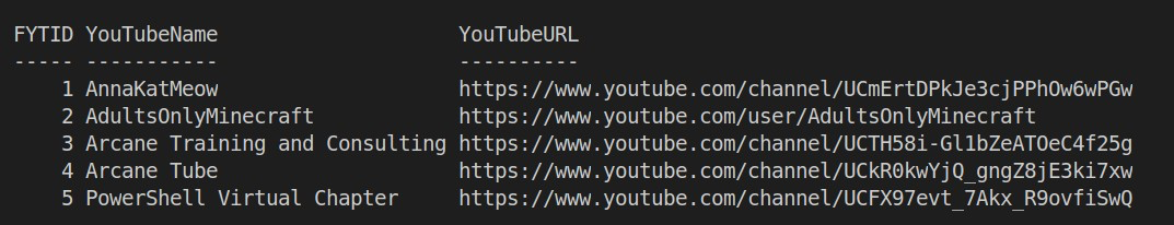
Here you can see each row of data, and the values for each column. I want to be very precise about what PowerShell returns.

This is a collection of data row objects. Each data row has properties and methods. The sqlserver module converts each column into a property of the data row object.

The majority of the time, you will want to work with the data returned to PowerShell, not just display it to the screen. To do so, first assign the output of Invoke-SqlCmd to a variable.

$data = Invoke-Sqlcmd -Query $sql @sqlParams

If you want to see the contents of the variable, simply run just the variable name.

$data

This will display the contents of the collection variable $data, displaying each row object, and the properties for each row.

You can also iterate over the $data collection, here’s a simple example.

foreach($rowObject in $data)
{
  "$($rowObject.YouTubeName) is a favorite YouTuber!"
}

This sample produces the following output:

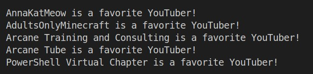
In this code, I just display a formatted text string, but you could do anything you want to with it, such as writing to an output file.

Cleanup

When I was a kid, mom always taught me to put my toys away. There are many reasons why you would want to remove containers you are no longer using. Testing is one, and you may wish to write a script to spin up a new container, load it with data, then let the testers do their thing. When done, you may wish to stop the container or delete it altogether.

Stopping and Starting Containers

For a first step, use Docker to see what containers are currently running.

sudo docker container ls

The output shows that on the system only one container is running.

Take the scenario of wanting to shut down the container, but not removing it. Perhaps you want to turn it off when the testers aren’t using it to save money and resources. To do this, simply use the stop command.

After issuing a stop, you should do another listing to ensure it is, in fact, stopped. You might think you could do another container ls, but note I said it lists currently running containers. If you want to see all containers, running or not, you must use a slightly different Docker command.

sudo docker stop arcanesql 
sudo docker ps -a

The stop command will stop the container with the name passed in. The ps -a command will list all containers running or not.

If you look at the STATUS column, on the very right side of the output, you’ll see the word Exited, along with how long in the past it exited. This is the indicator the container is stopped.

In this example, say it is the next morning. The testers are ready to get to work, so start the container back up.

sudo docker container start arcanesql

All that is needed is to issue the start command, specifying container, and provide the name of the container to start.

As you can see, the status column now begins with Up and indicates the length of time this container has been running.

Deleting a Container

At some point, you will be done with a container. Perhaps testing is completed, or you want to recreate the container, resetting it for the next round of testing.

Removing a container is even easier than creating it. First, you’ll need to reissue the stop command, then follow it with the Docker command to remove (rm) the named container.

sudo docker stop arcanesql 
sudo docker rm arcanesql

If you want to be conservative with you keystrokes, you can do this with a single command.

sudo docker rm --force arcanesql

The –force switch will make Docker stop the container if it is still running, then remove it.

You can verify it is gone by running or Docker listing command.

sudo docker ps -a

As you can see, nothing is returned. Of course, if you had other containers, they would be listed, but the arcanesql container would be gone.

Removing the Image

Removing the container does not remove the image the container was based on. Keeping the image can be useful for when you are ready to spin up a new container based on the image. Re-run the Docker listing command to see what images are on the system.

sudo docker image ls

The output shows the image downloaded earlier in this article.

As you can see, 1.3 GB is quite a bit of space to take up. In addition, you can see that the image was created 2 months ago. Perhaps a new one has come out, and you want to update to the latest—all valid reasons for removing the image.

To do so, use a similar pattern as the one for the container. You’ll again use rm, but specify it is an image to remove and specify the exact name of the image.

sudo docker image rm mcr.microsoft.com/mssql/server:2017-latest

When you do so, Docker will show us what it is deleting.

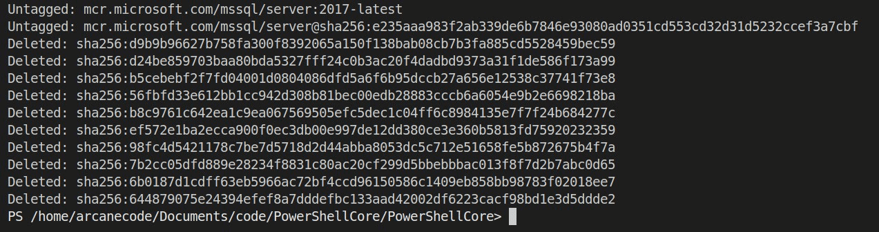
With that done, you can run another image listing using the image ls command to verify it is gone.

The image no longer appears. Of course, if you had other images you had downloaded, they would appear here, but the one for the latest version of SQL Server would be absent.

Conclusion

In this article, you saw how to use Docker, from within PowerShell Core, to download an image holding SQL Server 2017. You then created a container from that image.

For the next step, you installed the PowerShell SqlServer module, ran some queries to create a table and populate it with data. You then read the data back out of the database so you could work with it. Along the way, you learned the valuable concept of splatting.

Once finishing the work, you learned how to start and stop a container as well as remove it and the image on which it was based.

This article just scratched the service of what you can do when you combine Docker, SQL Server, and PowerShell Core. As you continue to learn, you’ll find even more ways to combine PowerShell Core, SQL Server and Docker.

The post How to Create an Ubuntu PowerShell Development Environment – Part 3 appeared first on Simple Talk.

from Simple Talk https://ift.tt/3evtkZI
via

Storage 101: Convergence and Composability

The series so far:

• Storage 101: Welcome to the Wonderful World of Storage
• Storage 101: The Language of Storage
• Storage 101: Understanding the Hard-Disk Drive 
• Storage 101: Understanding the NAND Flash Solid State Drive
• Storage 101: Data Center Storage Configurations
• Storage 101: Modern Storage Technologies
• Storage 101: Convergence and Composability 

These days, discussions around storage inevitably lead to the topics of convergence and composability, approaches to infrastructure that, when done effectively, can simplify administration, improve resource utilization, and reduce operational and capital expenses. These systems currently fall into three categories: converged infrastructure, hyperconverged infrastructure (HCI), and composable infrastructure.

Each infrastructure, to a varying degree, integrates compute, storage, and network resources into a unified solution for supporting various types of applications and workloads. Although every component is essential to operations, storage lies at the heart of each one, often driving the entire architecture. In fact, you’ll sometimes see them referred to as data storage solutions because of the vital role that storage plays in supporting application workloads.

Convergence and composability grew out of the need to address the limitations of the traditional data center, in which systems are siloed and often over-provisioned, leading to higher costs, less flexibility, and more complex management. Converged, hyperconverged, and composable infrastructures all promise to address these issues, but take different approaches to getting there. If you plan to purchase one of these systems, you need to understand those differences in order to choose the most effective solution for your organization.

Before discussing each infrastructure, review this matrix which summarizes the differences. 

Converged Infrastructure

A converged infrastructure consolidates compute, storage, network, and virtualization technologies into an integrated platform optimized for specific workloads, such as a database management system or virtual desktop infrastructure (VDI). Each component is prequalified, preconfigured, and assembled into a highly engineered system to provide a complete data solution that’s easier to implement and maintain than a traditional infrastructure.

The components that make up a converged infrastructure can be confined to a single rack or span multiple racks, depending on the supported workloads. Each component serves as a building block that works in conjunction with the other components to create a unified, integrated platform.

Despite this integration, each component remains a discrete resource. In this way, you can add or remove individual components as necessary, while still retaining the infrastructure’s overall functionality (within reason, of course). In addition, you can reuse a removed component for other purposes, an important distinction from HCI.

A converged infrastructure can support a combination of both hard-disk drives (HDDs) and solid-state drives (SSDs), although many solutions have moved toward all-flash storage. The storage is typically attached directly to the servers, with the physical drives pooled to create a virtual storage area network (SAN).

In addition to the hardware components, a converged infrastructure includes virtualization and management software. The platform uses the virtualization software to create resource pools made up of the compute, storage, and network components so they can be shared and managed collectively. Applications see the resources as pooled capacities, rather than individual components.

Despite the virtualization, the converged infrastructure remains a hardware-based solution, which means it doesn’t offer the agility and simplicity that come with software-defined systems such as hyperconverged and composable infrastructures. Even so, when compared to a traditional infrastructure, a converged infrastructure can help simplify management enough to make it worth serious consideration.

The components that make up a converged infrastructure are deployed as a single platform that’s accessible through a centralized interface for controlling and monitoring the various systems. In many cases, this eliminates the need to use the management interfaces available to the individual components. At the same time, you can still tune those components directly if necessary, adding to the system’s flexibility.

Another advantage to the converged infrastructure is that the components are prevalidated to work seamlessly within the platform. Not only does this help simplify procuring the components, but it also makes it easier to install them into the infrastructure, a process that typically takes only a few minutes. That said, it’s still important to validate any new storage you add to the infrastructure to ensure it delivers on its performance promises. Prevalidated components also reduce deployment risks because you’re less likely to run into surprises when you try to install them.

There are plenty of other advantages as well, such as quick deployments, reduced costs, easy scaling and compatibility with cloud computing environments. Even so, a converged infrastructure is not for everybody. Although you have flexibility within the platform’s structure, you have few options for altering the basic configuration, resulting in less flexibility should you want to implement newer application technologies.

In addition, a converged infrastructure inevitably leads to vendor lock-in. Once you’ve invested in a system, you’ve essentially eliminated products that are not part of the approved package. That said, you’d be hard-pressed to deploy any highly optimized and engineered system without experiencing some vendor lock-in.

If you choose a converged infrastructure, you have two basic deployment options. The first is to purchase or lease a dedicated appliance such as the Dell EMC VxBlock 1000. In this way, you get a fully configured system that you can deploy as soon as it arrives. The other option is to use a reference architecture (RA) such as the HP Converged Infrastructure Reference Architecture Design Guide. The RA provides hardware and configuration recommendations for how to assemble the infrastructure. In some cases, you can even use your existing hardware.

Hyperconverged Infrastructure

The HCI platform takes convergence to the next level, moving from a hardware-based model to a software-defined approach that abstracts the physical compute, storage, and (more recently) network components and presents them as shared resource pools available to the virtualized applications.

Hyperconvergence can reduce data center complexity even further than the converged infrastructure while increasing scalability and facilitating automation. HCI may add features such as data protection, data deduplication, intelligent management, and cloud bursting.

An HCI solution is typically made up of commodity compute, storage, and network components that are assembled into self-contained and highly integrated nodes. Multiple nodes are added together to form a cluster, which serves as the foundation for the HCI platform. Because storage is attached directly to each node, there is no need for a physical SAN or network area storage (NAS).

Each node runs a hypervisor, management software, and sometimes other specialized software, which work together to provide a unified platform that pools resources across the entire infrastructure. To scale out the platform, you simply add one or more nodes.

Initially, HCI targeted small-to-midsized organizations that ran specific workloads, such as VDI. Since then, HCI has expanded its reach to organizations of all sizes, while supporting a broader range of workloads, including database management systems, file and print services, email servers, and specialized solutions such as enterprise resource planning.

Like a converged infrastructure, a hyperconverged system offers a variety of benefits, beginning with centralized management. You can control all compute, storage and network resources from a single interface, as well as orchestrate and automate basic operations. In addition, an HCI solution reduces the amount of time and effort needed to manage the environment and carry out administrative tasks. It also makes it easier to implement data protections while ensuring infrastructure resilience.

An HCI solution typically comes as an appliance that is easy to deploy and scale. An organization can start small with two or three nodes (usually three) and then add nodes as needed, without a minimal amount of downtime. The HCI software automatically detects the new hardware and configures the resources. Upgrades are also easier because you’re working with a finite set of hardware/software combinations.

An HCI solution can integrate with other systems and cloud environments, although this can come with some fairly rigid constraints. Even so, the integration can make it easier to accommodate the platform in your current operations. The solution can also help reduce costs by simplifying administration and better utilization of resources while supporting the use of commodity hardware.

Despite these advantages, an HCI solution is not without its challenges. For example, vendor lock-in is difficult to avoid, as with the converged infrastructure, and HCI systems are typically preconfigured for specific workloads, which can limit their flexibility. In addition, nodes are specific to a particular HCI platform. You can’t simply pull a node out of the platform and use it for other purposes, nor can you add nodes from other HCI solutions.

HCI’s node-centric nature can also lead to over-provisioning. For example, you might need to increase storage and not computing. However, you can’t add one without the other. You must purchase a node in its entirety, resulting in more compute resources than you need. Fortunately, many HCI solutions now make it possible to scale compute and storage resources separately or have taken other steps to disaggregate resources. However, you’re still limited to a strictly-defined trajectory when scaling your systems.

You have three primary options for deploying an HCI solution. The first two are the same as a converged infrastructure. You can purchase or lease a preconfigured appliance, such as HPE SimpliVity, or you can use an RA, such as Lenovo’s Reference Architecture: Red Hat Hyperconverged Infrastructure for Virtualization. The third option is to purchase HCI software and build the platform yourself. For example, Nutanix offers its Acropolis software for deploying HCI solutions.

Composable Infrastructure

A composable infrastructure pushes beyond the limits of convergence and hyperconvergence by offering a software-defined infrastructure made up entirely of disaggregated, commodity components. The composable infrastructure abstracts compute, storage, and network resources and presents them as a set of unified services that can be allocated on-demand to accommodate fluctuating workloads. In this way, resources can be dynamically composed and recomposed as needed to support specific requirements.

You’ll sometimes see the term composable infrastructure used interchangeably with software-defined infrastructure (SDI) or infrastructure as code (IaC), implying that they are one in the same, but this can be misleading. Although a composable solution incorporates the principles of both, it would be more accurate to say that the composable infrastructure is a type of SDI that facilitates development methodologies such as IaC. In this sense, the composable infrastructure is an SDI-based expansion of IaC.

Regardless of the labeling, the important point is that a composable infrastructure provides a fluid pool of resources that can be provisioned on-demand to accommodate multiple types of workloads. A pool can consist of just a couple compute and storage nodes or be made up of multiple racks full of components. Organizations can assemble their infrastructures as needed, without the node-centric restrictions typical of HCI.

The composable infrastructure includes intelligent software for managing, provisioning, and pooling the resources. The software is programmable, self-correcting, and template-driven. The infrastructure also provides a standards-based management API for programmatically allocating (composing) resources. Administrators can use the API to control the environment, and developers can use the API to build resource requirements into their applications. The API also enables integration with third-party tools, making it possible to implement a high degree of automation.

A composable infrastructure can support applications running on bare metal, in containers, or in VMs. The infrastructure’s service-based model also makes it suitable for private or hybrid clouds and for workloads that require dynamic resource allocation, such as artificial intelligence (AI). In theory, a composable infrastructure could be made up of any commodity hardware components, and those components could span multiple locations. In reality, today’s solutions come nowhere close to achieving this level of agility, but like SDI, this remains a goal for many.

That said, today’s composable infrastructure solutions still offer many benefits, with flexibility at the top of the list. The infrastructure can automatically and quickly adopt to changing workload requirements, run applications in multiple environments (bare metal, containers, and VMs), and support multiple application types. This flexibility also goes hand-in-hand with better resource utilization. Resources can be scaled independently and provisioned based on workload requirements, without being tied to predefined blocks or nodes.

The composable platform also simplifies management and streamlines operations by providing a single infrastructure model that’s backed by a comprehensive API, which is available to both administrators and developers. IT teams can add components to the infrastructure in plug-and-play fashion, and development teams can launch applications with just a few clicks.

The composable infrastructure makes it possible to compose and decompose resources on demand, while supporting a high degree of automation and orchestration, as well as DevOps methodologies such as IaC. These benefits—along with increased flexibility and better resource utilization—can lead to lower infrastructure costs, in terms of both CapEx and OpEx.

However, the composable infrastructure is not without its challenges. As already pointed out, these systems have a long way to go to achieve the full SDI vision, leaving customers subject to the same vendor lock-in risks that come with converged and hyperconverged solutions.

In addition, the composable infrastructure represents an emerging market, with the composable software still maturing. The industry lacks agreed-upon standards or even a common definition. For example, HPE, Dell EMC, Cisco, and Liqid all offer products referred to as composable infrastructures but that are very different from one another, with each vendor putting its own spin on what is meant by composability.

No doubt the market will settle down at some point, and we’ll get a better sense of where composability is heading. In the meantime, you already have several options for deploying a composable infrastructure. You can purchase an appliance that comes ready to deploy, use a reference architecture like you would a blueprint, or buy composable software and build your own. Just be sure you do your homework before making any decisions so you know exactly what you’re getting for your money.

Converged to Composable and Beyond

Choosing a converged or composable infrastructure is not an all-or-nothing prospect. You can mix-and-match across your organization as best meets your requirements. For example, you might implement HCI systems in your satellite offices but continue to use a traditional infrastructure in your data center. In this way, you can easily manage the HCI platforms remotely and reduce the time administrators need to spend at those sites, while minimizing the amount of space being used at those locations.

Data and storage will play a pivotal role in any infrastructure decisions. To this end, you must take into account multiple considerations, including application performance, data protection, data quantities, how long data will be stored, expected data growth, and any other factors that can impact storage. You should also consider integration with other systems, which can range from monitoring and development tools to hybrid and public cloud platforms.

Of course, storage is only part of the equation when it comes to planning and choosing IT infrastructure. You must also consider such issues as deployment, management, scalability, resource consolidation, and the physical environment. But storage will drive many of your decisions, and the better you understand your data requirements, the more effectively you can choose an infrastructure that meets your specific needs.

The post Storage 101: Convergence and Composability appeared first on Simple Talk.

from Simple Talk https://ift.tt/2B347rc
via

Improve Row Count Estimates for Table Variables without Changing Code

You probably have heard that table variables work fine when the table variable only contains a small number of records, but when the table variable contains a large number of records it doesn’t perform all that well. A solution for this problem has been implemented in version 15.x of SQL Server (Azure SQL Database and SQL Server 2019) with the rollout of a feature called Table Variable Deferred Compilation

Table Variable Deferred Compilation is one of many new features to improve performance that was introduced in the Azure SQL Database and SQL Server 2019. This new feature was included in the Intelligent Query Processing (IQP). See Figure 1 for a diagram that shows all the IQP features introduced in Azure SQL Database and SQL Server 2019, as well as features that originally were part of the Adaptive Query Processing feature included in the older generation of Azure SQL Database and SQL Server 2017.

Figure 1: Intelligent Query Processing

In releases of SQL Server prior to 15.x, the database engine used a wrong assumption on the number of rows that were in a table variable. Because of this bad assumption, the execution plan that was generated didn’t work too well when a table variable contained lots of rows. With the introduction of SQL Server 2019, the database engine now defers the compilation of a query that uses a table variable until the table variable is used the first time. By doing this, the database engine can more accurately identify cardinality estimates for table variables. By having more accurate cardinality numbers, queries that have large numbers of rows in a table variable will perform better. Those queries will need to be running against a database with a database compatibility level set to 150 (version 15.x of SQL Server) to take advantage of this feature. To better understand how deferred compilation improves the performance of table variables that contain a large number of rows, I’ll run through an example, but first, I’ll discuss what is the problem with table variables in versions of SQL Server prior to version 15.x.

What is the Problem with Table Variables?

A table variable is defined using a DECLARE statement in a batch or stored procedure. Table variables don’t have distribution statistics and don’t trigger recompiles. Because of this, SQL Server is not able to estimate the number of rows in a table variable like it does for normal tables. When the optimizer compiles code that contains a table variable, prior to 15.x, it assumes a table is empty. This assumption causes the optimizer to compile the query using an expected row count of 1 for the cardinality estimate for a table variable. Because the optimizer only thinks a table variable contains a single row, it picks operators for the execution plan that work well with a small set of records, like the NESTED LOOPS operator for a JOIN operation. The operators that work well on a small number of records do not always scale well when a table variable contains a large number of rows. Microsoft documented this problem and recommends that temp tables might be a better choice than using a table variable that contains more than 100 rows. Additionally, Microsoft even recommends that if you are joining a table variable with other tables that you consider using the query hint RECOMPILE to make sure that table variables get the correct cardinality estimates. Without the proper cardinality estimates queries with large table variables are known to perform poorly.

With the introduction of version 15.x and the Table Variable Deferred Compilation feature, the optimizer delays the compilation of a query that uses a table variable until just before it is used the first time. This allows the optimizer to know the correct cardinality estimates of a table variable. When the optimizer has an accurate cardinality estimate, it has a good chance at picking execution plan operators that perform well for the number of rows in a table variable. In order for the optimizer to defer the compilation, the database must have its compatibility level set to 150. To show how deferred compilation of table variables work, I’ll show an example of this new feature in action.

Table Variable Deferred Compilation in Action

To understand how deferred compilation works, I will run through some sample code that uses a table variable in a JOIN operation. That sample code can be found in Listing 1.

Listing 1: Sample Test Code that uses Table Variable in JOIN operation

USE WideWorldImportersDW;
GO
DECLARE @MyCities TABLE ([City Key] int not null);
INSERT INTO @MyCities 
  SELECT [City Key] FROM Dimension.City;
SELECT O.[Order Key], TV.[City Key]
FROM Fact.[Order] as O INNER JOIN @MyCities as TV
ON O.[City Key] = TV.[City Key];

As you can see, this code uses the WideWorldImportersDW database, which can be downloaded here. In this script, I first declare my table variable @MyCities and then insert 116,295 rows from the Dimension.City table into the variable. That variable is then used in an INNER JOIN operation with the Fact.[Order] table.

To show the deferred compilation in action, I will need to run the code in Listing 1 twice. The first execution will be run against the WideWorldImportsDW using compatibility code 140, and the second execution will run against this same database using compatibility level 150. The script I will use to compare how table variables work, using the two difference compatibility levels, can be found in Listing 2.

Listing 2: Comparison Test Script

USE WideWorldImportersDW;
GO
-- Turn on time statistics
SET STATISTICS TIME ON; 
GO
---------------------------------------------------
-- Test #1 - Using SQL Server 2017 compatibility --
---------------------------------------------------
ALTER DATABASE WideWorldImportersDW SET COMPATIBILITY_LEVEL = 140;
GO
DECLARE @MyCities TABLE ([City Key] int not null);
INSERT INTO @MyCities 
  SELECT [City Key] FROM Dimension.City;
SELECT O.[Order Key], TV.[City Key]
FROM Fact.[Order] as O JOIN @MyCities as TV
ON O.[City Key] = TV.[City Key]
---------------------------------------------------
-- Test #2 - Using SQL Server 2019 compatibility --
---------------------------------------------------
ALTER DATABASE WideWorldImportersDW SET COMPATIBILITY_LEVEL = 150;
GO
USE WideWorldImportersDW;
GO
DECLARE @MyCities TABLE ([City Key] int not null);
INSERT INTO @MyCities 
  SELECT [City Key] FROM Dimension.City
SELECT O.[Order Key], TV.[City Key]
FROM Fact.[Order] as O JOIN @MyCities as TV
ON O.[City Key] = TV.[City Key];
GO

When I run the code in Listing 2, I run it from a query window in SQL Server Management Studio (SSMS), with the Include Actual Execution Plan query option turned on. The execution plan I get with I run query Test #1 and #2 can be found in Figure 2 and Figure 3, respectfully.

Figure 2: Execution Plan for Test #1 code in Listing 2, using compatibility level 140

Figure 3: Execution Plan for Test #2 code in Listing 2, using compatibility level 150

If you compare the execution plan between Figure 2 and 3, you will see the execution plans are a little different. When compatibility mode 140 was used, my test query used a NESTED LOOPS operation to join the table variable to the Fact.[Order] table, whereas when using compatibility mode 150, the optimizer picked a HASH MATCH operator for the join operation. This occurred because the Test #1 query uses an estimated row count of 1 for the table variable @MyCities. Whereas the Test #2 query was able to use the deferred table variable compilation feature which allowed the optimizer to use an estimated row count of 116,295 for the table variable. These estimated row count numbers can be verified by looking at the Table Scan operator properties for each execution plan, which are shown in Figure 4 and 5 respectfully.

Figure 4: Table Scan properties when Test #1 query ran under compatibility level 140

Figure 5: Table Scan properties when Test #2 query ran under compatibility level 150

By reviewing the table scan properties, the optimize used the correct estimated row count when compatibility level 150 was used. Whereas when compatibility level 140 was used, the optimizer estimated a row count of 1. Also note that my query that ran under compatibility level 150 also used BATCH mode for the TABLE SCAN operation, whereas the compatibility mode 140 query ran using ROW mode. You may be asking yourself now, how much faster does running my test code under compatibility level 150 perform over running the test code under the older compatibility level 140.

Comparing Performance between Compatibility Mode 140 and 150

In order to compare the performance of running my test query under both compatibility level, I executed the script in Listing 1 ten different times under each of the two compatibility levels. I then calculated the average CPU and elapsed time for the two different compatibility levels, and finally graphed the average performance number in the graph in Figure 6.

Figure 6: Performance Comparison between Compatibility Mode 140 and 150.

When the test query was run under compatibility mode 150, it used a fraction of the CPU over compatibility level 140. Whereas the Elapsed Time value of the test query that ran under compatibility level 150 ran 4.6 times faster than then using compatibility level 140. This is a significate performance improvement. But since batch mode processing was for the compatibility level 150 test, I can’t assume all this improvement was associated with only the Deferred Table Variable Compilation feature.

In order to remove the batch mode from my performance test, I’m going to run my test query under compatibility mode 150 one more time. But this time my test will run with a query hint to disable the batch mode feature. The script I will use for this additional test can be found in Listing 3.

USE WideWorldImportersDW;
GO
DECLARE @MyCities TABLE ([City Key] int not null);
INSERT INTO @MyCities 
  SELECT [City Key] FROM Dimension.City
SELECT O.[Order Key], TV.[City Key]
FROM Fact.[Order] as O JOIN @MyCities as TV
ON O.[City Key] = TV.[City Key]
OPTION(USE HINT('DISALLOW_BATCH_MODE'));
GO 10

Listing 3: Test #2 query with Batch Mode disabled

The graph in Figure 7 shows the new performance comparison results using deferred compilation and row mode features when my test ran under compatibility level 150.

Figure 7: Table Variable Deferred Compilation Comparison with Batch Mode disabled

With the Batch Mode feature disabled, my CPU went up significantly from my previous test when batch mode was enabled. But the Elapsed Time was only slightly different. Deferred Compilation seems to provide significate performance improvements, by delaying the compilation of a query until the table variable is used the first time. I have to wonder if the deferred compilation feature will improve the cardinality estimate issue caused by parameter sniffing with a parameterized query.

Does Deferred Compilation Help with Parameter Sniffing?

Parameter sniffing has been known to cause performance issues when a compiled execute plan is executed multiple times using different parameter values. But does the deferred table variable compilation feature in 15.x solve this parameter sniffing issue? To determine whether or not it does, let me create a stored procedure name GetOrders, to test this out. That stored procedure CREATE statement can be found in Listing 4.

Listing 4: Code to test out parameter sniffing

USE WideWorldImportersDW;
GO
CREATE OR ALTER PROC GetOrders(@CityKey int) 
AS
DECLARE @MyCities TABLE ([City Key] int not null);
INSERT INTO @MyCities 
  SELECT [City Key] FROM Dimension.City
  WHERE [City Key] < @CityKey;
SELECT *
FROM Fact.[Order] as O INNER JOIN @MyCities as TV
ON O.[City Key] = TV.[City Key]
GO

The number of rows returned by the stored procedure in Listing 4 is controlled by the value passed in the parameter @MyCities. To test if the deferred compilation feature solves the parameter sniffing issue, I will run the code in Listing 5.

Listing 5: Code to see if deferred compilation resolves parameter sniffing issue

USE WideWorldImportersDW;
GO
SET STATISTICS IO ON;
DBCC FREEPROCCACHE;
-- First Test
EXEC GetOrders @CityKey = 10;
--Second Test
EXEC GetOrders @CityKey = 231412;

The code in Listing 5 first runs the test stored procedure using a value of 10 for the parameter. The second execution uses the value 231412 for the parameter. These two different parameters will cause the store procedure to process drastically different numbers of rows. After I run the code in Listing 5, I will explore the execution plan for each execution of the stored procedure. I will look at the properties of the TABLE SCAN operation to see what the optimizer thinks are the estimated and actual rows count for the table variables for each execution. The table scan properties for each execution can be found in Figure 8 and 9 respectfully.

Figure 8: Table Scan Statistics for the first execution of the test stored procedure

Figure 9: Table Scan Statistics for the second execution of the test stored procedure

Both executions got the same number of estimated rows counts but got considerably different actual row counts. This means that the deferred table compilation feature of version 15.x doesn’t resolve the parameter sniffing problem of a stored procedure.

What Editions Supports the Deferred Compilations for Table Variables?

Like many cool new features that have come out with each new release of SQL Server in the past, they are first introduced in Enterprise edition only, and then over time, they might become available in other editions. You will be happy to know that the Deferred Compilation for Table Variables feature doesn’t follow this typical pattern. As of the RTM release of SQL Server 2019, the deferred compilation feature is available in all editions of SQL Server, as documented here.

Improve Performance of Code using Table Variables without Changing Any Code

TSQL code that contains a table variable has been known not to perform well when the variable contains lots of rows. This is because the code that declares the table valuable is compiled before the table has been populated with any rows of data. Well, that has all changed when TSQL code is executed in SQL Server 2019 or Azure SQL DB when your database is running under compatibility level 150. When using a database that is in compatibility level 150, the optimizer defers the compilation of code using a table variable until the first time the table variable is used in a query. By deferring the compilation, SQL Server can obtain a more accurate estimate of the number of rows in the table variable. When the optimizer has better cardinality estimates for a table variable, the optimizer can pick more appropriate operators for the execution plan, which leads to better performance. Therefore, if you have found code where table variables don’t scale well when they contain a lot of rows, then possibly version 15.x of SQL Server might help. By running TSQL code under compatibility level 150, you can improve the performance of code using table variables without changing any code.

 

The post Improve Row Count Estimates for Table Variables without Changing Code appeared first on Simple Talk.

from Simple Talk https://ift.tt/2ZKLEu5
via

Heaps in SQL Server: Part 1 The Basics

The series so far:

1. Heaps in SQL Server: Part 1 The Basics

This article is the beginning of a series of articles about Heaps in Microsoft SQL Server. Heaps are rejected by many database developers using Microsoft SQL Server. The concerns about Heaps are even fuelled by Microsoft itself by generally recommending the use of clustered indexes for every table. Globally renowned SQL Server experts also generally advise that tables in Microsoft SQL Server be provided with a clustered index.

Again, and again, I try to convince developers that a heap can even have advantages. I have discussed many pros and cons with these people and would now like to break a “PRO HEAP” lance. This article deals with the basics. Important system objects that play a major role in Heaps are only superficially presented in this article and described in detail in a follow up article.

The Basics of Heaps

Heaps are avoided in Microsoft SQL Server as the devil avoids holy water. One reason for the rejection is that many blog articles by renowned SQL Server Experts indicate that a table should use a clustered index. This article is the beginning of a series of articles that focuses on the broadest possible scope of application pro or con Heaps. The focus is on the heap to decide for yourself whether and when a heap has advantages or disadvantages compared to a clustered index. A sensible decision requires that you understand the way of working and the internal structures.

What are Heaps

Heaps are tables without a clustered index. Without an index, no sorting of the data is guaranteed. Data is stored in the table where there is space without a predetermined order. If the table is empty, data records are entered in the table in the order of the INSERT commands.

CREATE TABLE dbo.Customers
(
        Id      INT NOT NULL,
        Name    VARCHAR (200) NOT NULL,
        Street  VARCHAR (200) NOT NULL,
        Code    CHAR (3) NOT NULL,
        ZIP     VARCHAR (5) NOT NULL,
        City    VARCHAR (200) NOT NULL,
        State   VARCHAR (200) NOT NULL
)
GO
INSERT INTO dbo.Customers(Id, Name, Street, Code, Zip, City, State)
VALUES(1,'John Smith','Times Square','123','10001',
'New York','New York');

The script creates a new table for storing customer data and inserts one row. Since neither an index nor a primary key is used with the CLUSTERED option, data will be stored “unsorted” in this table.

If a table does not have a clustered index, the heap can be seen in the system view [sys]. [Indexes] which will always have the [Index_Id] = 0.

-- A Heap has always the index_id = 0
SELECT  object_id,
        name,
        index_id,
        type_desc
FROM    sys.indexes
WHERE   object_id = OBJECT_ID (N'dbo.Customers', N'U');
GO

Figure 1: [index_id] = 0 or [index_id] = 1 is reserved for Heaps OR Clustered Indexes

The Structure of Heaps

Since Heaps are primitive data stores, no complex structures are required to manage Heaps. Heaps have one row in sys.partitions, with [index_id] = 0 for each partition used by the Heap. When a Heap has multiple partitions, each partition has a Heap structure that contains the data for that specific partition.

Depending on the data types in the Heap, each Heap structure will have one or more allocation units to store and manage the data for a specific partition. At a minimum, each Heap will have one IN_ROW_DATA allocation unit per partition.

Figure 2: Storage concept of Heaps / Clustered Indexes / Nonclustered Indexes

Index Allocation Map

Each table and index use IAM structures (Index Allocation Map) to manage the data pages. An IAM page contains information about blocks (extents) that are used by a table or index per allocation unit.

Data pages of a Heap do not store references to next or previous data pages (links). This is not necessary for Heaps because a Heap does not require data to be sorted according to defined criteria.

SELECT     SIAU.type_desc,
       SIAU.total_pages,
       SIAU.used_pages,
       SIAU.data_pages,
       SIAU.first_iam_page,
        sys.fn_PhysLocFormatter(SIAU.first_iam_page) AS iam_page
FROM    sys.system_internals_allocation_units AS SIAU
        INNER JOIN sys.partitions AS P
        ON
                SIAU.container_id = 
                CASE WHEN SIAU.type IN (1, 3)
                  THEN P.hobt_id
                  ELSE P.partition_id
                END
WHERE   P.object_id = OBJECT_ID (N'dbo.Customers', N'U');
GO

The column [first_iam_page] in the [sys].[system_internals_allocation_units] system view points to the first IAM page in the chain of IAM pages that manage the allocated data pages of a Heap in a specific partition. Don’t worry about the mystic hex code; it can easily be deciphered with the function sys.fn_PhysLocFormatter!

Figure 3: Information about page allocations and first IAM page

The above query returns information about the storage type, number of pages and the location of the first IAM-page which manages the data pages of the Heap. Microsoft SQL Server only needs the first IAM page because it holds a reference to the next IAM and so on.

To have a look into the secrets of an IAM Page, you can use DBCC PAGE but be careful about using undocumented functions in a production system.

-- route the output of DBCC PAGE to the client
DBCC TRACEON (3604);
-- Show the content of a data page
DBCC PAGE (0, 1, 188, 3);

 

Figure 4: A deeper look into the content of an IAM-page

The above depiction shows the stored information in the IAM page of our Heap. It says that pages 32,680 – 32,967 are allocated by the table [dbo].[Customers]. So now Microsoft SQL Server knows what data pages hold data when running a SELECT statement against the Heap.

Page Free Space (PFS)

The fill level of a data page can only be specified for data pages of a Heap. Unlike a clustered index, the data rows are not sorted and do not have to be entered in a sorted form. It is up to Microsoft SQL Server to decide on which data page a data record is saved.

However, to assess where a record can be saved, Microsoft SQL Server needs to know where there is enough space on allocated data pages to complete the transaction. This information is retrieved via the recorded fill level of the data page. The information is held in the PFS page.

The problem is that this degree of filling is not saved “exactly”. Rather, Microsoft SQL Server only uses “rough” percentages to indicate the degree of filling.

The next higher fill level is updated as soon as the state is exceeded. For example, a data page is ALWAYS 50% full as soon as the first data record is entered.

The current fill level of data pages of a heap can be determined with the – undocumented – system function [sys]. [dm_db_database_page_allocations].

The next example shows how the fill level changes when the state (bytes) is exceeded. To do this, a Heap is created that stores 2,004 bytes per data record.

DROP TABLE IF EXISTS dbo.demo_table;
GO
CREATE TABLE dbo.demo_table
(
        C1      INT             NOT NULL        IDENTITY (1, 1),
        C2      CHAR(2000)      NOT NULL        DEFAULT ('Test')
);
GO
INSERT INTO dbo.demo_table DEFAULT VALUES;
GO

After the table has been created, insert one record into the table. Although the data page is filled with only 25%, Microsoft SQL Server records the filling status of the page with 50%.

-- What pages have been allocated?
SELECT  allocated_page_page_id,
        previous_page_page_id,
        next_page_page_id,
        page_type_desc,
        page_free_space_percent
FROM    sys.dm_db_database_page_allocations
(
        DB_ID(),
        OBJECT_ID(N'dbo.demo_table', N'U'),
        0,
        NULL,
        N'DETAILED'
);
GO

Figure 5: The page_free_space_percent

When you insert a second row the fill level won’t change since 2 * 2011 bytes = 4,022 bytes do not reach 50%. The fill level only needs to be updated for the third data record!

-- Insert a second row into the demo table
INSERT INTO dbo.demo_table DEFAULT VALUES;
GO

NOTE: Each data record has a record header that describes the structure of the data record. The structure is stored in 7 bytes. The physical length of a sample data record is therefore not 2,004 bytes but 2,011 bytes. To learn more about the anatomy of a record, read this article by Paul Randal.

Conclusion

This article described the internals of Heaps, but you may still be wondering if there are any advantages to using them. Here is a summary of the advantages and disadvantages which I’ll write about in future articles:

Advantages of Heaps

Using a heap can be more efficient than a table with a clustered index. In general, there are some use cases for Heaps like loading staging tables or storing protocol data into a Heap, since there is no need to pay attention to sorting when saving data. Data records are saved on the next possible data page on which there is sufficient space. Furthermore, the INSERT process does not require moving down the B-Tree of an index structure to the data page to save the record!

Disadvantages of Heaps

Heaps can have several disadvantages:

A Heap cannot scale if the database design is unsuitable because of PFS contention (will be handled in the next articles in detail!)

You cannot efficiently search for data in a Heap.

The time to search for data in a Heap increases linearly with the volume of data.

A Heap is unsuitable for frequent data updates because of the risk of forwarded records (will be handled in the next articles in detail)

A Heap is horrible for every database administrator when it comes to maintenance because a Heap requires an update of nonclustered indexes when the Heap is rebuilt.

Some of the “disadvantages” mentioned above can be eliminated or bypassed if you know how a heap “ticks” internally. I hope I can convince one or the other that a clustered index is not always the better choice. How to optimize the handling of Heaps will be described in future articles, so stay tuned!

 

The post Heaps in SQL Server: Part 1 The Basics appeared first on Simple Talk.

from Simple Talk https://ift.tt/2ANmGj3
via

Hands-On with Columnstore Indexes: Part 1 Architecture

Indexes are the key to efficient performance in any relational database. Few index enhancements have been introduced that can improve query speed and efficiency as dramatically as columnstore indexes.

Improvements to this feature have been introduced in each subsequent version of SQL Server and have transformed columnstore indexes into the go-to method of indexing OLAP workloads.

In this article, we will review the basics of columnstore indexes. In later articles, we will dive into best practices, and explore more advanced indexing considerations. I have personally had the pleasure of using columnstore indexes in a variety of applications, from small analytics tables to massive repositories and look forward to sharing my experiences (the good, the bad, and the silly).

As this article progresses through a discussion of columnstore indexes, the information presented will become more specific. Initially, an overview and generalized benefits will be discussed, followed by basic architecture and then increasingly more detail that builds upon previous ideas.

Test Data

Before diving into columnstore indexes, it is helpful to create a large table, index it, and use it throughout this article. Having a demo available in each section will aid in explaining how these indexes work and why they are so blazingly fast. It’ll also allow us to illustrate best practices and how not to use them. The WorldWideImportersDW sample database will be used for generating schema and data sets for us to work with.

The following T-SQL will create and populate a table with enough rows to illustrate columnstore index function effectively:

CREATE TABLE dbo.fact_order_BIG_CCI (
        [Order Key] [bigint] NOT NULL,
        [City Key] [int] NOT NULL,
        [Customer Key] [int] NOT NULL,
        [Stock Item Key] [int] NOT NULL,
        [Order Date Key] [date] NOT NULL,
        [Picked Date Key] [date] NULL,
        [Salesperson Key] [int] NOT NULL,
        [Picker Key] [int] NULL,
        [WWI Order ID] [int] NOT NULL,
        [WWI Backorder ID] [int] NULL,
        [Description] [nvarchar](100) NOT NULL,
        [Package] [nvarchar](50) NOT NULL,
        [Quantity] [int] NOT NULL,
        [Unit Price] [decimal](18, 2) NOT NULL,
        [Tax Rate] [decimal](18, 3) NOT NULL,
        [Total Excluding Tax] [decimal](18, 2) NOT NULL,
        [Tax Amount] [decimal](18, 2) NOT NULL,
        [Total Including Tax] [decimal](18, 2) NOT NULL,
        [Lineage Key] [int] NOT NULL);
INSERT INTO dbo.fact_order_BIG_CCI
SELECT
     [Order Key] + (250000 * ([Day Number] + 
        ([Calendar Month Number] * 31))) AS [Order Key]
    ,[City Key]
    ,[Customer Key]
    ,[Stock Item Key]
    ,[Order Date Key]
    ,[Picked Date Key]
    ,[Salesperson Key]
    ,[Picker Key]
    ,[WWI Order ID]
    ,[WWI Backorder ID]
    ,[Description]
    ,[Package]
    ,[Quantity]
    ,[Unit Price]
    ,[Tax Rate]
    ,[Total Excluding Tax]
    ,[Tax Amount]
    ,[Total Including Tax]
    ,[Lineage Key]
FROM Fact.[Order]
CROSS JOIN
Dimension.Date
WHERE Date.Date <= '2013-04-10'
CREATE CLUSTERED COLUMNSTORE INDEX CCI_fact_order_BIG_CCI 
ON dbo.fact_order_BIG_CCI WITH (MAXDOP = 1);

The resulting table, dbo.fact_order_BIG, contains 23,141,200 rows, which provides enough data to experiment on and demo the performance of columnstore indexes. For most analytic workloads, the clustered columnstore index is all that is needed, but there can be value in adding non-clustered rowstore indexes to satisfy specific OLTP querying needs. These are typically added on a case-by-case basis as they will add additional storage, memory, and processing footprints to the table.

To provide some side-by-side comparisons, the following T-SQL will create an additional test table that utilizes a classic BIGINT identity-based clustered index. An additional non-clustered index is created on [Order Date Key] to facilitate searches by date.

CREATE TABLE dbo.fact_order_BIG (
        [Order Key] [bigint] NOT NULL 
           CONSTRAINT PK_fact_order_BIG PRIMARY KEY CLUSTERED,
        [City Key] [int] NOT NULL,
        [Customer Key] [int] NOT NULL,
        [Stock Item Key] [int] NOT NULL,
        [Order Date Key] [date] NOT NULL,
        [Picked Date Key] [date] NULL,
        [Salesperson Key] [int] NOT NULL,
        [Picker Key] [int] NULL,
        [WWI Order ID] [int] NOT NULL,
        [WWI Backorder ID] [int] NULL,
        [Description] [nvarchar](100) NOT NULL,
        [Package] [nvarchar](50) NOT NULL,
        [Quantity] [int] NOT NULL,
        [Unit Price] [decimal](18, 2) NOT NULL,
        [Tax Rate] [decimal](18, 3) NOT NULL,
        [Total Excluding Tax] [decimal](18, 2) NOT NULL,
        [Tax Amount] [decimal](18, 2) NOT NULL,
        [Total Including Tax] [decimal](18, 2) NOT NULL,
[Lineage Key] [int] NOT NULL);
INSERT INTO dbo.fact_order_BIG
SELECT
         [Order Key] + (250000 * ([Day Number] + 
          ([Calendar Month Number] * 31))) AS [Order Key]
    ,[City Key]
    ,[Customer Key]
    ,[Stock Item Key]
    ,[Order Date Key]
    ,[Picked Date Key]
    ,[Salesperson Key]
    ,[Picker Key]
    ,[WWI Order ID]
    ,[WWI Backorder ID]
    ,[Description]
    ,[Package]
    ,[Quantity]
    ,[Unit Price]
    ,[Tax Rate]
    ,[Total Excluding Tax]
    ,[Tax Amount]
    ,[Total Including Tax]
    ,[Lineage Key]
FROM Fact.[Order]
CROSS JOIN
Dimension.Date
WHERE Date.Date <= '2013-04-10';
CREATE NONCLUSTERED INDEX IX_fact_order_BIG 
ON dbo.fact_order_BIG ([order date key]);

Columnstore Indexes: An Overview

Columnstore indexes take much of what we know about data storage and querying in SQL Server and turn it on its head. Many of the conventions we are used to following with regards to developing T-SQL, contention, and optimization do not apply here.

It is important to note that columnstore indexes are built for tables that are very large. If a table will not contain millions or billions of rows, then it will not fully benefit from it. In general, the larger a table, the more the columnstore index will speed it up.

Columnstore indexes are designed to support analytics in SQL Server. Prior to this feature, tables with billions of rows were cumbersome and challenging to query with adequate speed and efficiency. We were often forced to pre-crunch many fact tables up-front to answer the questions we might ask later. This process drove business intelligence in SQL Server for years. It also drove many analysts out of SQL Server and into SQL Server Analysis Services or a variety of 3^rd party tools.

As data grew exponentially, there was a strong desire to be able to maintain detailed fact data that can be targeted directly with reports and analytics. Columnstore indexes can provide speed boosts of 10x-100x or more for typical OLAP queries. This analysis will start with clustered columnstore indexes, as they offer the most significant boost to performance for OLAP workloads. Here are the reasons why such impressive speeds can be attained:

Compression

By storing data grouped by columns, like values can be grouped together and therefore compress very effectively. This compression will often reduce the size of a table by 10x and offers significant improvements over standard SQL Server compression.

For example, if a table with a billion rows has an ID lookup column that has 100 distinct values, then on average each value will be repeated 10 million times. Compressing sequences of the same value is easy and results in a tiny storage footprint.

Just like standard compression, when columnstore data is read into memory, it remains compressed. It is not decompressed until runtime when needed. As a result, less memory is used when processing analytic queries. This allows more data to fit in memory at one time, and the more operations that can be performed in memory, the faster queries can execute.

Compression is the #1 reason why columnstore indexes are fast. The tiny storage and memory footprint allow massive amounts of data to be read and retained in memory for analytics. Consider the size of the table that we created above:

305MB for 23 million rows is quite impressive! Fact.Order contains 1/100 of the data, but consumes 55MB:

Multiplying by 100 and dividing by the columnstore index size, we can approximate a compression ratio of 18-to-1. This is partly due to the effective compression achieved by columnstore indexes, but also because there is little to no need for additional covering non-clustered indexes.

Inline Metadata

As part of compression, metadata is collected about the underlying data. This allows metrics such as row counts, minimum values, maximum values, and data size to be stored inline with the compressed data. The result is the ability to generate aggregate metrics very quickly as there is no need to scan the detail data to generate these calculations.

For example, the simplest calculation of COUNT(*) in an OLTP table requires a clustered index scan, even though no column data is being returned. The following query returns a count from our new table:

SELECT
                COUNT(*)
FROM dbo.fact_order_BIG_CCI;

It runs exceptionally fast, requiring only 116 logical reads. Note the details of the execution plan:

Traditionally, we have been trained to recoil at the thought of clustered index scans, but with columnstore indexes, this will typically be the operator that is used. For compressed OLAP data, scanning a large range of data is expected and normal. The index is optimized for this behavior and is no more afraid of large numbers than we should be 😊

Taking a look at STATISTICS IO, we can verify that the new index uses very little IO:

Table ‘fact_order_BIG_CCI’. Scan count 1, logical reads 0, physical reads 0, page server reads 0, read-ahead reads 0, page server read-ahead reads 0, lob logical reads 116, lob physical reads 1, lob page server reads 0, lob read-ahead reads 0, lob page server read-ahead reads 0.

Table ‘fact_order_BIG_CCI’. Segment reads 23, segment skipped 0.

SQL Server can satisfy the count using metadata from the index, rather than needing to count each and every row in the index. The following is IO on the OLTP variant of the table:

Table ‘fact_order_BIG’. Scan count 5, logical reads 49229, physical reads 1, page server reads 0, read-ahead reads 48746, page server read-ahead reads 0, lob logical reads 0, lob physical reads 0, lob page server reads 0, lob read-ahead reads 0, lob page server read-ahead reads 0.

49229 reads vs. 116 is a massive difference. More advanced queries and concepts will be introduced later. In general, expect aggregate queries that operate over a large set of rows to perform far more efficiently with a columnstore index.

Batch Execution

When columnstore indexes were introduced, Microsoft also debuted batch mode processing. This is a method of executing a query where rows are processed in groups, rather than row-by-row in a single thread. Prior to SQL Server 2016, this required the server’s maximum degree of parallelism to be set to a value other than 1 and for the query to use parallel processing and therefore take advantage of batch mode. Starting in SQL Server 2016, SQL Server added the ability for batch mode to operate as a serial process, processing batches of rows utilizing a single CPU rather than many. Parallelism can still be applied to a query, but it is no longer a requirement for batch mode to be used.

The resulting performance will be greatly improved as SQL Server can read batches of data into memory without the need to pass control back and forth between operators in the execution plan. Whether batch mode is used or not can be verified by checking the properties for any execution plan operator:

For any analytics query across a large volume of data, expect batch mode to be used. The query optimizer will typically choose batch or row mode correctly given the:

• Table schema
• Query structure
• Server settings

If a query against a columnstore index is preforming poorly and row mode is being used, then investigation is warranted to determine the cause. Perhaps not enough CPUs were available or the maximum degree of parallelism was set to 1 (prior to SQL Server 2016). Otherwise, check the database’s compatibility level to ensure it is set high enough to take advantage of the batch mode features available in the server’s SQL Server version.

Bulk Loading

To facilitate speedy loading of large volumes of data into a columnstore index, SQL Server will use a bulk load process to populate rowgroups whenever possible. This allows data to be moved directly into the columnstore index via a minimally logged process.

For a reporting database, this is ideal as logging every row inserted is time-consuming and likely unnecessary in an OLAP environment. There is no need to specify a bulk load process when loading data into a columnstore index.

Columnstore Index Architecture

Physically, data is stored in rowgroups, which consist of up to 1,048,576 (2²⁰) rows. Each rowgroup is subdivided into column segments, one per column in the table. The column segments are then compressed and stored on pages. The resulting structure can be visualized like this:

Each segment contains metadata about the data contained within, allowing many aggregate operations to be performed without reading a million distinct values. If a segment or set of segments contain no values that satisfy a query, then it can be skipped. The process of skipping unneeded rowgroups is called rowgroup elimination, and is one of two important ways that columnstore indexes are architected to reduce the amount of data that needs to be scanned to satisfy a query.

Because columnstore indexes separate each column into its own compressed structure, any columns not needed for a query can be ignored. The process of skipping unneeded columns is called segment elimination and allows large portions of a table to be ignored when only a few columns are needed.

Rowgroup structures can be viewed using the dynamic management view sys.column_store_row_groups:

SELECT
        tables.name AS table_name,
        indexes.name AS index_name,
        partitions.partition_number,
        column_store_row_groups.row_group_id,
        column_store_row_groups.state_description,
        column_store_row_groups.total_rows,
        column_store_row_groups.size_in_bytes
FROM sys.column_store_row_groups
INNER JOIN sys.indexes
ON indexes.index_id = column_store_row_groups.index_id
AND indexes.object_id = column_store_row_groups.object_id
INNER JOIN sys.tables
ON tables.object_id = indexes.object_id
INNER JOIN sys.partitions
ON partitions.partition_number = 
     column_store_row_groups.partition_number
AND partitions.index_id = indexes.index_id
AND partitions.object_id = tables.object_id
WHERE tables.name = 'fact_order_BIG_CCI'
ORDER BY tables.object_id, indexes.index_id, 
column_store_row_groups.row_group_id;

Joining this new view to some additional system views provides a simple result set that tells us about columnstore index rowgroups:

There are a total of 23 row groups within this columnstore index, of which the above image shows the last six. Note that all but the final rowgroup contain the maximum allowed number of rows that can be inserted into a rowgroup. This is optimal and exactly what we want when building a columnstore index. This optimization will be discussed in further detail when index write operations are delved into later in this article.

Similarly, we can view metadata about segments within each rowgroup using another dynamic management view: sys.column_store_segments.

SELECT
        tables.name AS table_name,
        indexes.name AS index_name,
        columns.name AS column_name,
        partitions.partition_number,
        column_store_segments.segment_id,
        column_store_segments.row_count,
        column_store_segments.has_nulls,
        column_store_segments.on_disk_size
FROM sys.column_store_segments
INNER JOIN sys.partitions
ON column_store_segments.hobt_id = partitions.hobt_id
INNER JOIN sys.indexes
ON indexes.index_id = partitions.index_id
AND indexes.object_id = partitions.object_id
INNER JOIN sys.tables
ON tables.object_id = indexes.object_id
INNER JOIN sys.columns
ON tables.object_id = columns.object_id
AND column_store_segments.column_id = columns.column_id
WHERE tables.name = 'fact_order_BIG_CCI'

This query returns a row per segment, allowing you to analyze the contents of a columnstore index for each column. This can help determine which columns compress most (or least) effectively, as well as keep track of the size and structure of a columnstore index on a more granular scale:

The Deltastore

Writing to a highly compressed object is an expensive operation. Because of this, SQL Server contains a separate structure for managing some of the changes to the columnstore index: The deltastore. This adds another component to the previously presented image of a columnstore index:

In contrast to the columnstore index, the deltastore is a classic B-tree clustered index. The minimum number of rows that can be bulk loaded into a rowstore is 102,400. When less rows are inserted, they are placed first into the deltastore, which will continue to accumulate rows until there are enough to merge into the columnstore index and the deltastore is closed.

The process that merges data from a deltastore into the columnstore index is called the tuple-mover and is an automated background process that will perform its work without operator intervention. It is possible to influence this process and move closed deltastores into the columnstore index via index rebuild/reorg operations. This will be discussed in greater detail below.

When a query is executed against the columnstore index, it will interrogate both the compressed rowgroups as well as the deltastore. The result set will be a combination of data from each. A query that needs to retrieve data from the deltastore will inherently be a bit slower as it needs to traverse a B-Tree structure in addition to the more efficient columnstore index.

With a classic heap or clustered index, large inserts could cause contention on the base table. As a result, database administrators would often perform inserts in smaller batches to reduce the size and duration of individual operations to ensure that the underlying table remains available for other operations. This reduced transaction log size, as well as the length of locks against the underlying data as it was being written to.

One of the most important takeaways of this process is that the optimal way to load data into a columnstore index is in large batches. Inserting data in small batches provides no value and will slow down data loads, as the deltastore will get used as an intermediary between your source data and the columnstore index.

An optimal data load size is 1,048,576 rows as that would completely fill up a rowstore within the clustered index. Some administrators will intentionally save data to intentionally load only the maximum rowstore size each time. This is optimal, but also a hassle. Realistically, the most convenient way to manage data loads is through a combination of large data loads and periodic index maintenance.

Delete Operations

Unlike inserts, which can benefit from bulk loading large row counts, deletes are solely managed through the deltastore. When a row is deleted, it is marked in the deltastore for deletion. The row remains in the columnstore index and the tuple-mover processes and flags them as deleted.

This can be demonstrated by performing a delete of 100 rows from the clustered columnstore index created above:

DELETE
FROM dbo.fact_order_BIG_CCI
WHERE fact_order_BIG_CCI.[Order Key] >= 8000001
AND fact_order_BIG_CCI.[Order Key] < 8000101;

We can review the results by checking a new column from sys.column_store_row_groups:

SELECT
        tables.name AS table_name,
        indexes.name AS index_name,
        partitions.partition_number,
        column_store_row_groups.row_group_id,
        column_store_row_groups.state_description,
        column_store_row_groups.total_rows,
        column_store_row_groups.size_in_bytes,
        column_store_row_groups.deleted_rows
FROM sys.column_store_row_groups
INNER JOIN sys.indexes
ON indexes.index_id = column_store_row_groups.index_id
AND indexes.object_id = column_store_row_groups.object_id
INNER JOIN sys.tables
ON tables.object_id = indexes.object_id
INNER JOIN sys.partitions
ON partitions.partition_number = column_store_row_groups.partition_number
AND partitions.index_id = indexes.index_id
AND partitions.object_id = tables.object_id
WHERE tables.name = 'fact_order_BIG_CCI'
ORDER BY indexes.index_id, column_store_row_groups.row_group_id;

The results tell us exactly where in the columnstore index rows have been flagged for deletion:

The deleted_rows column indicates how many rows have been soft-deleted. This query can be expanded slightly to expose the columnstore index delete bitmap object used for flagging these 100 rows as deleted:

SELECT
        tables.name AS table_name,
        indexes.name AS index_name,
        partitions.partition_number,
        column_store_row_groups.row_group_id,
        column_store_row_groups.state_description,
        column_store_row_groups.total_rows,
        column_store_row_groups.size_in_bytes,
        column_store_row_groups.deleted_rows,
        internal_partitions.partition_id,
        internal_partitions.internal_object_type_desc,
        internal_partitions.rows
FROM sys.column_store_row_groups
INNER JOIN sys.indexes
ON indexes.index_id = column_store_row_groups.index_id
AND indexes.object_id = column_store_row_groups.object_id
INNER JOIN sys.tables
ON tables.object_id = indexes.object_id
INNER JOIN sys.partitions
ON partitions.partition_number = column_store_row_groups.partition_number
AND partitions.index_id = indexes.index_id
AND partitions.object_id = tables.object_id
LEFT JOIN sys.internal_partitions
ON internal_partitions.object_id = tables.object_id
AND column_store_row_groups.deleted_rows > 0
WHERE tables.name = 'fact_order_BIG_CCI'

ORDER BY indexes.index_id, column_store_row_groups.row_group_id;

The results add a bit more information:

Sys.internal_partitions exposes the structure used for managing the soft deletes. While this will be academic in nature for most operators, it is important to stress the nature of delete and update operations against columnstore indexes. That is: They are more complex than insert and select operations.

Note that rows are NEVER deleted from a columnstore index. They are flagged as deleted, but not removed. The cost to decompress a rowgroup and recompress it again is high and the only way to eliminate this technical debt is to rebuild the index (or the partition containing the deleted data).

Caution should be used when performing delete or update operations as they incur additional overhead in later updating the compressed columnstore index structure. In addition, delete and update operations can cause fragmentation if they change data in a way that results in the natural ordering of data within the index being disrupted. Similarly, a columnstore index can become less efficient over time if rowstores are deleted from repeatedly, as the result will be more and more rowstores with less rows in each to manage. The concept of order in a columnstore index will be discussed shortly and is critically important for making the most efficient use of it.

Update Operations

In a classic heap or clustered B-tree, an update is modelled as a delete followed immediately by an insert. The operations are carried out immediately in order, committed, and logged. Typically, these updates will not be slower than running an insert or delete operation independently of each other.

The deltastore adds an extra later of complexity that results in an update operation being modelled as two independent write operations that depend upon each other, both of which are committed to the deltastore. This is a very expensive operation, and will usually be significantly slower and less efficient than issuing separate delete and insert operations instead. For a large columnstore index, the cost of an update can be crippling to a database server – even one with significant resources allocated to it.

The following is an example of an update operation against a columnstore index:

UPDATE fact_order_BIG_CCI
        SET Quantity = 1
FROM dbo.fact_order_BIG_CCI
WHERE fact_order_BIG_CCI.[Order Key] >= 8000101
AND fact_order_BIG_CCI.[Order Key] < 8000106;

This query will update 5 rows, changing the quantity to 1 for each. By modifying the columnstore DMV query used previously, the results can be filtered to only show data that has yet to be fully committed to the columnstore index:

SELECT
        tables.name AS table_name,
        indexes.name AS index_name,
        partitions.partition_number,
        column_store_row_groups.row_group_id,
        column_store_row_groups.state_description,
        column_store_row_groups.total_rows,
        column_store_row_groups.size_in_bytes,
        column_store_row_groups.deleted_rows,
        internal_partitions.partition_id,
        internal_partitions.internal_object_type_desc,
        internal_partitions.rows
FROM sys.column_store_row_groups
INNER JOIN sys.indexes
ON indexes.index_id = column_store_row_groups.index_id
AND indexes.object_id = column_store_row_groups.object_id
INNER JOIN sys.tables
ON tables.object_id = indexes.object_id
INNER JOIN sys.partitions
ON partitions.partition_number = column_store_row_groups.partition_number
AND partitions.index_id = indexes.index_id
AND partitions.object_id = tables.object_id
LEFT JOIN sys.internal_partitions
ON internal_partitions.object_id = tables.object_id
AND column_store_row_groups.deleted_rows > 0
WHERE tables.name = 'fact_order_BIG_CCI'
AND column_store_row_groups.state_description = 'OPEN'
OR (column_store_row_groups.deleted_rows IS NOT NULL 
    AND column_store_row_groups.deleted_rows > 0)
ORDER BY indexes.index_id, column_store_row_groups.row_group_id;

The results show 2 additional changes:

The total deleted rows count is now 105 (up from 100) and two additional entries appear in the deltastore that account for both deletes and inserts against the columnstore index.

Deltastore Summary

The primary takeaway of how the deltastore works is that larger data loads are better and delete/update operations should be minimized and isolated as much as possible. We will dig further into specific operations and performance in later articles in this series, which will allow us to further understand the most optimal ways to create columnstore indexes, load data into them, and maintain them.

When designing a large table to use a columnstore index, take extra time to design out updates and minimize delete operations. Doing so will make data loads faster, reduce the need for index maintenance, and improve the performance of select queries against the table.

Conclusion

Columnstore indexes are an impressive feature that has grown and improved with each release of SQL Server since its inception. To take full advantage of columnstore indexes, though, requires understanding how data is stored in them to determine best practices for efficiently loading and reading data.

Additional concepts such as data order, partitioning, segment elimination, and rowgroup elimination can allow OLAP data access to be significantly more efficient and scalable as data continues to grow. In the next article, I’ll cover some of these best practices and guidelines.

 

The post Hands-On with Columnstore Indexes: Part 1 Architecture appeared first on Simple Talk.

from Simple Talk https://ift.tt/2WQc8s3
via