Are your Oracle archived log files much too small?

Have you ever noticed that your archived redo logs can be much smaller than the online redo logs and may display a wild variation in size? This difference is most likely to happen in systems with a very large SGA (system global area), and the underlying mechanisms may result in Oracle writing data blocks to disc far more aggressively than is necessary. This article is a high-level description of how Oracle uses its online redo logs and why it can end up generating archived redo logs that are much smaller than you might expect.

Background

I’ll start with some details about default values for various instance parameters, but before I say any more, I need to present a warning. Throughout this article, I really ought to keep repeating “seems to be” when making statements about what Oracle is (seems to be) doing. Because I don’t have access to any specification documents or source code, all I have is a system to experiment on and observe and the same access to the documentation and MOS as everyone else. However, it would be a very tedious document if I had to keep reminding you that I’m just guessing (and checking). I will say this only once: remember that any comments I make in this note are probably close to correct but aren’t guaranteed to be absolutely correct. With that caveat in mind, start with the following (for 19.3.0.0):

Processes defaults to cpu_count * 80 + 40

Sessions defaults to processes * 1.5 + 24 (the manuals say + 22, but that seems to be wrong)

Transactions: defaults to sessions * 1.1

The parameter I’ll be using is transactions. Since 10g, Oracle has allowed multiple “public” and “private” redo log buffers, generally referred to as strands; the number of private strands is trunc(transactions/10). and the number of public strands is trunc(cpu_count/16) with a minimum of 2. In both cases, these are maximum values, and Oracle won’t necessarily use all the strands (and may not even allocate memory for all the private strands) unless there is contention due to the volume of concurrent transactions.

For 64-bit systems, the private strands are approximately 128KB and, corresponding to the private redo strands, there is a set of matching in-memory undo structures which are also approximately 128KB each. There are x$ objects you can query to check the maximum number of private strands but it’s easier to check v$latch_children as there’s a latch protecting each in-memory undo structure and each redo strand:

select  name, count(*) 
from    v$latch_children
where   name in (
                'In memory undo latch',
                'redo allocation'
        )
group by name
/

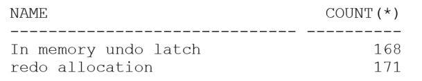
The difference between the number of redo allocation latches and in-memory undo latches tells you that I have three public redo strands on this system as well as the 168 (potential) private strands.

The next important piece of the puzzle is the general strategy for memory allocation. To allow Oracle to move chunks of memory between the shared pool and buffer cache and other large memory areas, the memory you allocate for the SGA target is handled in “granules” so, for example:

select  component, current_size, granule_size 
from    v$sga_dynamic_componentsa
where   current_size != 0
/

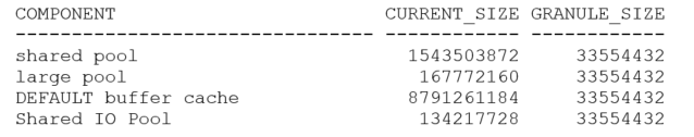
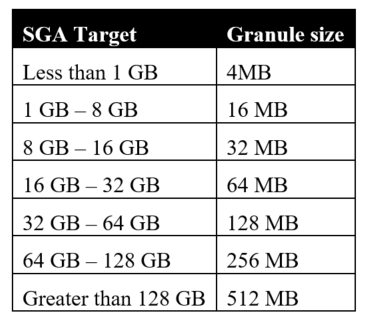
This is a basic setup with a 10GB SGA target, with everything left to default. As you can see from the final column, Oracle has decided to handle SGA memory in granules of 32MB. The granule size is dependent on the SGA target size according to the following table:

The last piece of information you need is the memory required for the “fixed SGA” which is reported as the “Fixed size” as the instance starts up or in response to the command show sga (or select * from v$sga), e.g.:

SQL> show sga

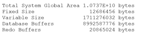
Once you know the granule size, the fixed SGA size, and the number of CPUs (technically the value of the parameter cpu_count rather than the actual number of CPUs) you can work out how Oracle calculates the size of the individual public redo strands – plus or minus a few KB.

By default, Oracle allocates a single granule to hold both the fixed SGA and the public redo strands, and the number of public redo strands is trunc(cpu_count/16). With my cpu_count of 48, a fixed SGA size of 12,686,456 bytes (as above), and a granule size of 33,554,432 bytes (32MB), I should expect to see three public redo strands sized at roughly:

(33,554,432 – 12,686,456) / trunc((48 / 16)) = 20,867,976 / 3 = 6,955,992

In fact, you’ll notice if you start chasing the arithmetic, that the numbers won’t quite match my predictions. Some of the variations are due to the granule map, and other headers, pointers and other things I don’t know about in the granule that holds the fixed SGA and public redo buffers. In this case, the actual reported size of the public strands was 6,709,248 bytes – so the calculation is in the right ballpark but not extremely accurate.

Log buffer, meet log file

It is possible to set the log_buffer parameter in the startup file to dictate the space to be allocated to the public strands. It’s going to be convenient for me to do so to demonstrate why the archived redo logs can vary so much in size for “no apparent reason”. Therefore, I’m going to restart this instance with the setting log_buffer = 60M. This will (should) give me 3 public strands of 20MB. But 60MB is more than one granule, and if you add the 12MB fixed size that’s 72MB+. This result is more than two granules, so Oracle will have to allocate three granules (96MB) to hold everything. This is what I see as the startup SGA:

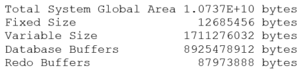
Checking the arithmetic 87973888 + 12685456 = 100659344 = 95.996 MB i.e. three granules.

The reason why I wanted a nice round 20MB for the three strands is that I created my online redo log files at 75MB (which is equivalent to 3 strands worth plus 15MB), and then I decided to drop them to 65MB (three strands plus 5MB).

My first test consisted of nothing but switching log files then getting one process to execute a pl/sql loop that did several thousand single-row updates and commits. After running the test, this is what the last few entries of my log archive history looked like:

select  sequence#, blocks, blocks * block_size / 1048576 
from    v$archived_log;

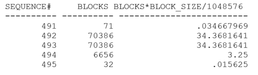
My test generated roughly 72MB of redo, but Oracle switched log files (twice) after a little less than 35MB. That’s quite interesting, because 34.36 MB is roughly 20MB (one public strand) + 15MB and that “coincidence” prompted me to reduce my online logs to 65MB and re-run the test. This is what the next set of archived logs looked like:

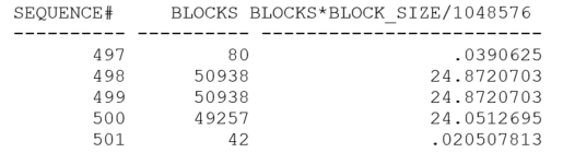
This time I have archived logs which are about 25MB – which is equivalent to one strand plus 5MB – and that’s a very big hint. Oracle is behaving as if each public strand allocates space for itself in the online redo log file in chunks equal to the size of the strand. Then, when the strand has filled that chunk, Oracle tries to allocate the next chunk – if the space is available. If there’s not enough space left for a whole strand, Oracle allocates the rest of the file. If there’s no space left at all, Oracle triggers a log file switch, and the strand allocates its space in the next online redo log file. The sequence of events in my case was that each strand allocated 20MB, but only one of my strands was busy. When it had filled its first allocation, it allocated the last 5 (or 15) MB in the file. When that was full, I saw a log file switch.

To test this hypothesis, I could predict that if I ran two copies of my update loop (addressing 2 different tables to avoid contention), I would see the archived logs coming out at something closer to 45MB (i.e. two full allocations plus 5MB). Here’s what I got when I tried the experiment:

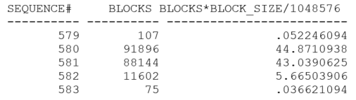
If you’re keeping an eye on the sequence# column, you may wonder why there’s been a rather large jump from the previous test. It’s because my hypothesis was right, but my initial test wasn’t quite good enough to demonstrate it. With all my single-row updates and commits and the machine I was using, Oracle needed to take advantage of the 2^nd public redo strand some of the time but not for a “fair share” of the updates. Therefore, the log file switch was biased towards the first public redo strand reaching its limits, and this produced archived redo logs of a fairly regular 35MB (which would be 25MB for public strand #1 and 10MB for public strand #2). It took me a few tests to realize what had happened. The results above come from a modified test where I changed the loop to run a small number of times updating 1,000 rows each time. I checked that I still saw switches at 25MB with a single run – though, as you may have noticed, the array update generated a lot less redo than the single-row updates to update the same number of rows.

Finally, since I had three redo strands, what’s going to happen if I run three copies of the loop (addressing three different tables)?

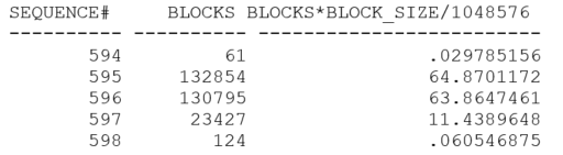
With sufficient pressure on the redo log buffers (and probably with just a little bit of luck in the timing), I managed to get redo log files that were just about full when the switch took place.

Consequences

Reminder – my description here is based on tests and inference; it’s not guaranteed to be totally correct.

When you have multiple public redo strands, each strand allocates space in the current online redo log file equivalent to the size of the strand, and the memory for the strand is pre-formatted to include the redo log block header and block number. When Oracle has worked its way through the whole strand, it tries to allocate space in the log file for the next cycle through the strand. If there isn’t enough space for the whole strand, it allocates all the available space. If there’s no space available at all, it initiates a log file switch and allocates the space from the next online redo log file.

As a consequence, if you have N public redo strands and aren’t keeping the system busy enough to be using all of them constantly, then you could find that you have N-1 strand allocations that are virtually empty when the log file switch takes place. If you are not aware of this, you may see log file switches taking place much more frequently than you expect, producing archived log files that are much smaller than you expect. (On the damage limitation front, Oracle doesn’t copy the empty parts of an online redo log file when it archives it.)

In my case, because I had created redo log files of 65MB then set the log_buffer parameter to 60MB when the cpu_count demanded three public redo strands, I was doomed to see log file switches every 25MB. I wasn’t working the system hard enough to keep all three strands busy. If I had left the log buffer to default (which was a little under 7MB), then in the worst-case scenario I would have left roughly 14MB of online redo log unused and would have been producing archived redo logs of 51MB each.

Think about what this might mean on a very large system. Say you have 16 Cores which are pretending to be 8 CPUs each (fooling Oracle into thinking you have 128 CPUs), and you’ve set the SGA target to be 100GB. Because the system is a little busy, you’ve set the redo log file size to be a generous-sounding 256MB. Oracle will allocate 8 public redo strands (cpu_count/16), and – checking the table above – a granule size of 256MB. Can you spot the threat when the granule size matches the file size, and you’ve got a relatively large number of public redo strands?

Assuming the fixed SGA size is still about 12M (I don’t have a machine I can test on), you’ve got

strand size = 244MB / 8 = 30.5 MB

When you switch into a new online redo log file, you pre-allocate 8 chunks of 30.5MB for a total of 244M, with only 12MB left for the first strand to allocate once it’s filled its initial allocation. The worst-case scenario Is that you could get a log file switch after only 30.5 MB + 12 MB = 42.5 MB. You could be switching log files about 6 times as often as expected when you set up the 256MB log file size.

Conclusion

There may be various restrictions or limits that make some difference to the arithmetic I’ve discussed. For example, I have seen a system using 512MB granules that seemed to set the public strand size to 32 MB when I was expecting the default to get closer to 64MB. There are a number of details I’ve avoided commenting on in this article, but the indications from the tests that I can do suggest that if you’re seeing archived redo log files that are small compared to the online redo log files, then the space you’re losing is because of space reserved for inactive or “low-use” strands. If this is the case, there’s not much (legal) that you can do other than increase the online redo log files so that the “lost” space (which won’t change) becomes a smaller fraction of the total size of the online redo log. As a guideline, setting the online redo log file size to at least twice the granule size seems like a good idea, and four times the size may be even better.

There are other options, of course, that involve tweaking the parameter file. Most of these changes would be for hidden parameters, but you could supply a suitable setting for the log_buffer parameter that makes the individual public strands much smaller – provided this didn’t introduce excessive waits for log buffer space. Remember that the value you set would be shared between the public redo threads, and don’t forget that the number of public redo threads might change if you change the number of CPUs in the system.

 

The post Are your Oracle archived log files much too small? appeared first on Simple Talk.

from Simple Talk https://ift.tt/36oNXpz
via

Why installing a “cringe-meter” on social media can boost joy

Do you cringe while scrolling through social media? When have you ever felt better after scrolling?

If you feel like social media is a net-loss for collective mental health, you’re not alone.

We post in superabundance with flailing emotions. We flaunt our duck-faced selfies with smooth-faced filters until we don’t even look human. We hammer our political stances down the throats of others until both sides are fuming. We show off our eighth-graders consolation sports awards as if they were the NBA finals. We highlight all of our greatness under a golden spotlight and ignore the flaws. The cringe-factor on social media has reached profound levels.

We’ve all done it. We’ve all made cringe-posts.

I’ve looked back at posts I’d made and had to cringe. You know the ones…

“Congratulations to me!” is the underlying theme of a cringe-post.

There’s nothing inherently wrong with self-promotion in the modern age, but these cringe-posts typically cross the line into “corn-syrup”. Cringe-posts are void of substance and social nutrition. They highlight thy self while providing no value to anyone else. Cringe-posts merely add to the noise and inject more “corn syrup” into the social media diet of others.

It’s a post made from a place of desperation or vulnerability. And it’s not our fault.

Those Instagram, Facebook and Twitter algorithms aim to exploit us when we are most vulnerable. We know this now. They nudge us to post more than we actually want to. And when we post too often, we run out of things to say. When we run out of things to say, we make posts without substance…cringe-posts. It’s not a good look for us as individuals.

This is why I have installed a cringe-meter into my social media. The meter runs 1-5.

1 = tiny bit cringe
2 = uncomfortable cringe
3 = gross cringe
4 = heavy reputation harming cringe
5 = unbearable career-threatening cringe

How does it work?

A close friend of whom I deeply trust will post a 1-5 in the comments of a “cringe-post” I make. And I will do the same for them. I call this person my “cringe-meter-monitor” (CMM). The goal is not to chart at all (no number posted in the comments).

It’s important to find a cringe-meter-monitor who will give it to you straight—someone with high self-awareness and higher social-awareness. Someone you really trust to critique you. Note, if they are posting several “cringe-posts” on their own social media, they are not the monitor for you.

So far, social media has been the old Wild West. And the cringe-meter is a system of checks and balances to restore some calm in the saloon.

Even if the cringe-meter can decrease cringes by 10-15%, I believe social media will be a much healthier and tolerable place: Less “corn syrup” posts. Less selfish posts. More posts made from a peaceful mindset. Quality over quantity.

Hey, the cringe-meter may not save the world, but it’s a solid start.

The good news is, social media has been exposed. At its core, it is ultimately not our friend. And with this new awareness, we can be more self-aware in how we present ourselves online. It’s all going to get better.

Commentary Competition

Enjoyed the topic? Have a relevant anecdote? Disagree with the author? Leave your two cents on this post in the comments below, and our favourite response will win a $50 Amazon gift card. The competition closes two weeks from the date of publication, and the winner will be announced in the next Simple Talk newsletter.

The post Why installing a “cringe-meter” on social media can boost joy appeared first on Simple Talk.

from Simple Talk https://ift.tt/39c6cQB
via

Developing a backup plan

The most important task for a DBA is to be able to recover a database in the event of a database becoming corrupted. Corrupted databases can happen for many different reasons. The most common corruption problem is from a programming error. But databases can also be corrupted by hardware failures. Regardless of how a database becomes corrupt, a DBA needs to have a solid backup strategy to be able to restore a database, with minimal data loss. In this article, I will discuss how to identify backup requirements for a database, and then how to take those requirements to develop a backup strategy.

Why develop a backup plan?

You might be wondering why you need to develop a backup plan. Can’t a DBA just implement a daily backup of each database and call it good? Well, that might work, but it doesn’t consider how an application uses a database. If you have a database that is only updated with a nightly batch process, then having a daily backup of the database right after the nightly update process might be all that you need. But what if you had a database that was updated all day long from some online internet application. If you have only one backup daily for a database that gets updated all day online, then you might lose up to a day’s worth of online transactions if it was to fail right before the next daily backup. Losing a day’s worth of transaction most likely would be unacceptable. Therefore, to ensure minimal data loss occurs when restoring a database, the backup and recovery requirements should be identified first before building a backup solution for a database.

Identifying backup and recovery requirements

Each database may have different backup and recovery requirements. When discussing backup and recovery requirements for a database, there are two different types of requirements to consider. The first requirement is how much data can be lost in the event of a database becoming corrupted. Knowing how much data can be lost will determine the types of database backups you need to take, and how often you take those backups. This requirement is commonly called the recovery point objective (RPO).

The second backup requirement to consider is how long it will take to recover a corrupted database. This requirement is commonly called the recovery time objective (RTO). The RTO requirement identifies how long the database can be down while the DBA is recovering the database. When defining the RTO, make sure to consider more than just how long it takes to restore the databases. Other tasks take time and need to be considered. Things like identifying which backup files need to be used, finding the backup files, building the restore script/process, and communicating with customers.

A DBA should not identify the RTO and RPO in a vacuum. The DBA should consult each application owner to set the RTO and RPO requirements for each database the application uses. The customers are the ones that should drive the requirements for RTO and RPO, with help from the DBA of course. Once the DBA and the customer have determined the appropriate RTO and RPO then, the DBA can develop the backups needed to meet these requirements.

Types of backups to consider

There are a number of different backup types you could consider. See my previous article for all the different backup types. Of those different backup types, there are three types of backups that support most backup and recovery strategies. Those types are Full, Differential, and Transaction log.

The Full backup, as it sounds, is a backup that copies the entire database off to a backup device. The backup will contain all the used data pages for the database. A full backup can be used to restore the entire database to the point in time that the full backup completed. I say completed because, if update commands are being run against the database at the time the backup is running, then they are included in the backup. Therefore, when you restore from a full backup, you are restoring a database to the point-in-time that the database backup completes.

A differential backup is a backup that copies all the changes since the last full backup off to a backup device. Differential backups are useful for large databases, where only a small number of updates have been performed since the full backup. Differential backups will run faster and take up less space on the backup device. A differential backup can’t be used to restore a database by itself. The differential backup is used in conjunction with a full backup to restore a database to the point in time that the differential backup completed. This means the full backup is restored first, then followed by restoring the differential backup.

The last type of backup is a transaction log backup. A transaction log backup copies all the transaction in the transaction log file to a backup device. It also removes any completed transactions from the transaction log to keep it from growing out of control. A transaction log backup, like a differential type backup, can’t be used by itself to restore a database. It is used in conjunction with a full backup, and possibly a differential backup to restore a database to a specific point-in-time. The advantages of having a transaction log backup are you can tell the restore process to stop at any time during the transaction log backup. By using the stop feature, you can restore a database right up to the moment before a database got corrupted. Typically, transaction logs are taken frequently, so there might be many transaction log backups taken between each full or differential backup. Transaction log backups are beneficial for situations when there is a requirement of minimal data loss in the event of a database becoming corrupted.

Developing a backup strategy for a database

When determining a backup plan for a database, you need to determine how much data can be lost and how long it takes to recover the database. This is where the RTO and RPO come in to determine which types of database backups should be taken. In the sections below, I will outline different database usage situations and then discuss how one or more of the backup types could be used to restore the database to meet the application owner’s RTO and RPO requirements.

Scenario #1: Batch updates only

When I say “Batch Updates Only”, I am referring to a database that is only updated using a batch process. Meaning it is not updated online or by using an ad hoc update processes. One example of this type of database is a database that receives updates in a flat-file format from a third-party source on a schedule. When a database receives updates via a flat-file, those updates are applied to the database using a well-defined update process. The update process is typically on a schedule to coincide with when the flat-file is received from the third-party source. In this kind of update situation, the customer would have an RPO that would be defined something like this: “In the event of a corrupted database, the database would need to be restored to after the last batch update process”. And would have an RTO set to something like this: “The restore process needs to be completed within X number of hours”.

When a database is only updated with a batch process, that is run on a schedule, all you need is to have a full back up right after the database has been updated. By doing this, you can recover to a point in time right after the database has been updated. Using the full backup only will meet the RPO. Since the time needed to restore a full backup is about the same time as it takes to backup, the RTO needs to be at least as long as it takes to run a restore process, plus a little more time for organizing and communicating a restore operation.

Scenario #2 – Batch updates only, with short backup window

This scenario is similar to the last scenario, but in this situation, there is very little time to take a backup after the batch processing completes. The time it takes to back up a database is directly proportional to the amount of data that needs to be backed up. If the time for a backup is short, it might be too short to take a full back up every time the database is updated. This might be the case when the database is very, very large. If there isn’t time to do a full database backup and the amount of data updated is small, then a differential backup would be a good choice to meet the RPO/RTO requirements. With a differential backup, only the updates since the last full backup are copied to the backup device. Because only the updates are backed up and not the entire database, a differential backup can run much faster than a full backup. Keep in mind, to restore a differential backup, you must first restore the full backup. In this situation, a full backup needs to be taken periodically with differential backups being taken in between the full backups. A common schedule for this would be to take the full backup when there is a large batch window, like on a Sunday when there is no batch processing, and then differential backups during those days when the batch window is short.

Scenario #3 – Ad hoc batch updates only

Some databases are not updated on a schedule but instead are updated periodically but only by an ad hoc batch update process that is manually kicked off. In this situation, there are a couple of different ways of handling backing up of databases that fall into this category. The first one is just routinely to run full database backups on a schedule. The second is to trigger a backup as the last step of the ad hoc batch update process.

A routine scheduled full backup is not ideal because the backups may or may not be run soon after the ad hoc batch update process. When there is a period of time between the ad hoc process and the scheduled full backup, the database is vulnerable to data loss should the database become corrupted for some reason before the full backup is taken. In order to minimize the time between the ad hoc update and the database backup, it would be better to add a backup command to the end of the ad hoc update process. This way, there is a backup soon after the ad hoc process, which minimizes the timeframe for when data could be lost. Additionally, by adding a backup command to the ad hoc update process, you potentially take fewer backups, which reduces the processing time and backup device space, over a routine backup process.

Scenario #4 – Online updates during business hours

In this scenario, the database gets updates from online transactions, but these online transactions are only run during business hours, say 8 AM to 5 PM. Outside of regular business hours, the database is not updated. In this situation, you might consider a combination of two different types of backups: Full and Transaction log backups. The full backup would be run off-hours, meaning after 5 PM and before 8 AM. The transaction log backups will be used during business hours to back up the online transactions shortly after these transactions have been made. In this situation, you need to review the RPO to determine how often to run transaction log backups. The shorter the RPO, the more often you need to take transaction log backups. For example, suppose a customer says they can lose no more than an hour worth of transactions, then you need to run a transaction log backup every hour between the hours of 8 AM and 5 PM.

Scenario #5 – Online updates 24×7

Some databases are accessed every day all day. This is very similar to Scenario #4, but in this case, the database is accessed and updated online 24×7. To handle backup and recovery in this situation, you would take a combination of full and differential backups along with transaction log backups.

With a database that is updated 24×7, you want to run the full and differential backups at times when the databases have the least number of online updates happening. By doing this, the performance impact caused by the backups will be minimized. There are way too many different database situations to tell you exactly how often a full or differential backup should be taken. I would recommend you try to take a full backup or differential backup daily if that is possible. By doing it daily, you will have fewer backup files involved in your recovery process.

The transaction log backups are used to minimize data loss. Like scenario #4, the frequency of transaction log backups is determined by the RPO requirements. Assuming that the customer can lose one hour’s worth of transitions, then transaction log backup would need to be run hourly, all day, every day to cover the 24×7 online processing.

Developing a backup plan

It is important for a DBA to work with the application owners to identify the backup and recovery requirements for their databases. The application owners determine how much data they can lose (RPO), and how long the database can be down while it is being recovered (RTO). Once the RTO and RPO requirements are defined, the DBA can then develop a backup plan that aligns with these requirements.

 

The post Developing a backup plan appeared first on Simple Talk.

from Simple Talk https://ift.tt/3fnQF1o
via

Normal Forms

Everyone gives lip service to normalized databases. But the truth is that normalization is a lot more complicated than most people know. First of all, I’ll bet almost no one reading this article (including me!) could name and define all of the current Normal Forms. Thankfully, you don’t really need all of the complexity that is possible. Let’s back up a step and ask, “why do you want to normalize database?” as opposed to just using a plain old file system.

The original Normal Forms were created by Dr. Codd in 1970. He borrowed this term because at the time, we were trying to “normalize relations” with the Soviet Union when it still existed.

Even before RDBMS, we had network and hierarchical databases. Their first goal was to remove redundancy. We want to store one fact, one way, one place, and one time. Normalization goes a step further. The goal of normalization is to prevent anomalies in the data. An anomaly could be an insertion anomaly, update anomaly, or deletion anomaly. This means that doing one of those basic operations destroys a fact or creates a falsehood.

Normal Forms

Let’s just start off with a list of the current Normal Forms defined in the literature. Some of them are obscure, and you probably won’t ever run into them, but they’re nice to know.

0NF: Unnormalized Form
1NF: First Normal Form
2NF: Second Normal Form
3NF: Third Normal Form
EKNF: Elementary Key Normal Form
BCNF: Boyce–Codd Normal Form
4NF: Fourth Normal Form
ETNF: Essential Tuple Normal Form
5NF: Fifth Normal Form
DKNF: Domain-Key Normal Form
6NF: Sixth Normal Form

I’m not going to discuss all of these normal forms, nor am I going to go into a lot of detail. I just want you to be aware of them.

First Normal Form (1NF)

Zero or Un-Normal Form is just in the list for completeness and to get a starting point. Normal Forms are built on top of each other. The idea is that if a table is in (n)th Normal Form, then it’s automatically also in (n-1)th Normal Form. The convention is that we begin with the First Normal Form. What’s remarkable is that people don’t get this right after all these decades. There are three properties a table must have to be in 1NF.

1) The table needs a PRIMARY KEY, so there are no duplicate rows. Here’s where we get into problems. By definition, a key is a minimal subset of columns that uniquely identifies each row. If it has too many columns, the subset is called a super key. Later, we realized that the key is a key, and there’s nothing special about a PRIMARY KEY, but that term (and SQL syntax) have become part of the literature because that’s how sequential files had to be organized before RDBMS. Sequential files can be sorted only one way, and each position referenced in that sorted order only one way. Tape files and punch card data processing depended on sorted order, and we spent a lot of time physically doing that sorting. This is just how we thought of processing data before we had random-access, good hashing and other tricks for data retrieval.

There’s also nothing to stop the table from having more than one key or keys with multiple columns. In a file system, each file is pretty much unrelated to any other file, but in a relational model, the tables are not standalone but have relationships among themselves.

Programmers learning RDBMS forget that a key must be made up of values taken from columns in the rows of the table. This means we do not use things like the IDENTITY table property or a physical disk location as a key. It’s clearly not an attribute of the entities being modeled by the table, but something that comes from a physical storage method.

2) No repeating groups are allowed. A repeating group is a subset of columns that store an array record structure or some other “non-flat” data structure. For example, FORTRAN and other procedural languages have arrays. COBOL, Pascal and PL/1 allow one record to contain multiple occurrences of the same kind of data. In COBOL, there’s a keyword OCCURS <n> TIMES that marks a repeated structure. The C family uses struct {..} for records and square brackets for arrays.

In the old days, we referred to files whose records all had the same simple structure as a flat file. Older programmers sometimes think that SQL was based on a flat file, and they did not have to unlearn the techniques they had in their toolbox already. Wrong. Flat files had no constraints or interrelationships, while tables do. Anytime you see someone writing SQL where there are no REFERENCES, CHECK() or DEFAULT clauses in their DDL, they probably learned to program on old flat file systems.

3) All of the values stored in the columns of a row are atomic. This means I cannot take them apart without destroying some of the meaning. In SQL, there is a big difference between a field and a column. Read the ANSI/ISO Standards; the term field refers to part of a column which can be used by itself. For example, a date column is made up of three fields: year, month, and day. In order to get a date, you have to have all three fields, but you can still get information from each field.

Consider a requirement to maintain data about class schedules at a school. We are required to keep the (course_name, class_section, dept_name, class_time, room_nbr, professor_name, student_id, student_major, student_grade) as a record. Let’s build a file first. I’m going to use Pascal because even if you’ve never written in it, you can almost immediately read it. The only things you need to know when you’re reading it is that:

1) ARRAY [i:j] OF <data type> declares an array with explicit upper and lower bounds and its data type. In particular, ARRAY [1:n] OF CHAR is how they represent a string of characters.

2) The RECORD..END construct marks a record.

3) You can nest them to create an array of records, a record with arrays, etc.

Here’s a possible declaration of a student classes file in Pascal:

Classes = RECORD
 course_name: ARRAY [1:7] OF CHAR;
 class_section: CHAR;
 class_time_period: INTEGER;
 room_nbr: INTEGER;
 room_size: INTEGER;
 professor_name: ARRAY [1:25] OF CHAR;
 dept_name: ARRAY [1:10] OF CHAR;
 students: ARRAY [1:class_size]
 OF RECORD
         student_id ARRAY [1:5] OF CHAR;
         student_major ARRAY [1:10] OF CHAR;
         student_grade CHAR;
         END;
 END;

This table is not yet in First Normal Form (1NF). The Pascal file could be “flattened out” into SQL to look like this:

CREATE TABLE Classes
(course_name CHAR(7) NOT NULL,
 class_section CHAR(1) NOT NULL,
 class_time_period INTEGER NOT NULL,
 room_nbr INTEGER NOT NULL,
 room_size INTEGER NOT NULL,
 professor_name CHAR(25) NOT NULL,
 dept_name CHAR(10) NOT NULL,
 student_id CHAR(5) NOT NULL,
 student_major CHAR(10) NOT NULL,
 student_grade CHAR(1) NOT NULL,
 PRIMARY KEY (course_name, class_section, student_id));

This table is acceptable to SQL. In fact, we can locate a row in the table with a combination of (course_name, class_section, student_id), so we have a key. But what we are doing is hiding the original Students record array, which has not changed its nature by being flattened.

There are problems.

If Professor ‘Jones’ of the Mathematics department dies, we delete all his rows from the Classes table. This also deletes the information that all his students were taking a Mathematics class and maybe not all of them wanted to drop out of school just yet. I am deleting more than one fact from the database. This is called a deletion anomaly.

If student ‘Wilson’ decides to change one of his Mathematics classes, formerly taught by Professor ‘Jones’, to English, we will show Professor ‘Jones’ as an instructor in both the Mathematics and the English departments. I could not change a simple fact by itself. This creates false information and is called an update anomaly.

If the school decides to start a new department, which has no students yet, we cannot put in the data about the professor_name we just hired until we have classroom and student data to fill out a row. I cannot insert a simple fact by itself. This is called an insertion anomaly.

There are more problems in this table, but you see the point. Yes, there are some ways to get around these problems without changing the tables. We could permit NULLs in the table. We could write triggers to check the table for false data. These are tricks that will only get worse as the data and the relationships become more complex. The solution is to break the table up into other tables, each of which represents one relationship or simple fact.

Second Normal Form (2NF)

Dr. Codd also introduced some mathematical notation for discussing relational theory. A single headed arrow can be read as determines, a key type of relationship. A double-headed arrow says the left-hand expression determines a subset of the right-hand expression. A “bowtie” is a symbol for doing a join on the left and right expressions. Let’s not worry about the bowtie for now, but you might want to remember that this was the original symbol in ANSI X3 flowchart symbols for a file merge.

A table is in Second Normal Form (2NF) if it is in 1NF and has no partial key dependencies. That is, if X and Y are columns and X is a key, then for any Z that is a proper subset of X, it cannot be the case that Z → Y. Informally, the table is in 1NF and it has a key that determines all non-key attributes in the table.

In the Pascal example, our users tell us that knowing the student_ID and course_name is sufficient to determine the class_section (since students cannot sign up for more than one class_section of the same course_name) and the student_grade. This is the same as saying that (student_id, course_name) → (class_section, student_grade).

After more analysis, we also discover from our users that (student_id → student_major) assuming that students have only one major. Since student_id is part of the (student_id, course_name) key, we have a partial key dependency! This leads us to the following decomposition:

CREATE TABLE Classes
(course_name CHAR(7) NOT NULL,
 class_section CHAR(1) NOT NULL,
 class_time_period INTEGER NOT NULL,
 room_nbr INTEGER NOT NULL,
 room_size INTEGER NOT NULL,
 professor_name CHAR(25) NOT NULL,
PRIMARY KEY (course_name, class_section));
CREATE TABLE Enrollment
(student_id CHAR(5) NOT NULL
  REFERENCES Students (student_id),
 course_name CHAR(7) NOT NULL,
 class_section
CHAR(1) NOT NULL,
 student_grade CHAR(1) NOT NULL,
PRIMARY KEY (student_id, course_name));
CREATE TABLE Students
(student_id CHAR(5) NOT NULL PRIMARY KEY,
 student_major CHAR(10) NOT NULL);

At this point, we are in 2NF. Every attribute depends on the entire key in its table. Now if a student changes majors, it can be done in one place. Furthermore, a student cannot sign up for different sections of the same class, because we have changed the key of Enrollment. Unfortunately, we still have problems.

Notice that while room_size depends on the entire key of Classes, it also depends on room_nbr. If the room_nbr is changed for a course_name and class_section, we may also have to change the room_size, and if the room_nbr is modified (we knock down a wall), we may have to change room_size in several rows in Classes for that room_nbr.

Third Normal Form (3NF)

The next Normal Form can address these problems. A table is in Third Normal Form (3NF) if it is in 2NF, and all the non-key columns are determined by “the key, the whole key, and nothing but the key. So help you, Codd.” This cute little slogan is due to Chris Date, not me.

The usual way that 3NF is explained is that there are no transitive dependencies, but this is not quite right. A transitive dependency is a situation where we have a table with columns (A, B, C) and (A → B) and (B → C), so we know that (A → C). In our case, the situation is that (course_name, class_section) → room_nbr and room_nbr → room_size. This is not a simple transitive dependency, since only part of a key is involved, but the principle still holds. To get our example into 3NF and fix the problem with the room_size column, we make the following decomposition:

CREATE TABLE Rooms
(room_nbr INTEGER NOT NULL PRIMARY KEY,
 room_size INTEGER NOT NULL);
CREATE TABLE Students
(student_id CHAR(5) NOT NULL PRIMARY KEY,
 student_major CHAR(10) NOT NULL);
CREATE TABLE Classes
(course_name CHAR(7) NOT NULL,
 class_section CHAR(1) NOT NULL,
 PRIMARY KEY (course_name, class_section),
 class_time_period INTEGER NOT NULL,
 room_nbr INTEGER NOT NULL
 REFERENCES Rooms(room_nbr));
CREATE TABLE Enrollment
(student_id CHAR(5) NOT NULL
 REFERENCES Students(student_id),
 course_name CHAR(7) NOT NULL,
 PRIMARY KEY (student_id, course_name),
 class_section CHAR(1) NOT NULL,
 FOREIGN KEY (course_name, class_section)
 REFERENCES Classes(course_name, class_section),
 student_grade CHAR(1) NOT NULL);

A common misunderstanding about relational theory is that 3NF tables have no transitive dependencies. As indicated above, if X → Y, X does not have to be a key if Y is part of a key. We still have a transitive dependency in the example — (room_nbr, class_time_period) → (course_name, class_section) — but since the right side of the dependency is a key, it is technically in 3NF. The unreasonable behavior that this table structure still has is that several course_names can be assigned to the same room_nbr at the same class_time.

Another form of transitive dependency is a computed column. For example:

CREATE TABLE Boxes
(width INTEGER NOT NULL,
 length INTEGER NOT NULL,
 height INTEGER NOT NULL,
 volume INTEGER NOT NULL
 CHECK (width * length * height = volume),
 PRIMARY KEY (width, length, height));

The volume column is determined by the other three columns, so any change to one of the three columns will require a change to the volume column. You can use a computed column in this example which would look like:

(volume INTEGER COMPUTED AS (width * length * height) PERSISTENT)

Elementary Key Normal Form (EKNF)

Elementary Key Normal Form (EKNF) is a subtle enhancement on 3NF. By definition, EKNF tables are also in 3NF. This happens when there is more than one unique composite key and they overlap. Such cases can cause redundant information in the overlapping column(s). For example, in the following table, let’s assume that a course code is also a unique identifier for a given subject in the following table:

CREATE TABLE Enrollment
(student_id CHAR(5) NOT NULL,
 course_code CHAR(6) NOT NULL,
 course_name VARCHAR(15) NOT NULL,
 PRIMARY KEY (student_id, course_name),
 UNIQUE (student_id, course_code) --- alternative key
);

This table, although it is in 3NF, violates EKNF. The PRIMARY KEY of the above table is the combination of (student_id, course_name). However, we can also see an alternate key (student_id, course_code) as well. The above schema could result in update and deletion anomalies because values of both course_name and course_code tend to be repeated for a given subject.

The following schema is a decomposition of the above table in order to satisfy EKNF:

CREATE TABLE Subjects
(course_code CHAR(6) NOT NULL PRIMARY KEY,
 course_name VARCHAR(15) NOT NULL);
CREATE TABLE Enrollment
(student_id CHAR(5) NOT NULL
 REFERENCES Students(student_id),
 course_code CHAR(6) NOT NULL
 REFERENCES Subjects(course_code),
 PRIMARY KEY (student_id, course_code));

 

For reasons that will become obvious in the following section, ensuring a table is in EKNF is usually skipped, as most designers will move directly on to Boyce-Codd Normal Form after ensuring that a schema is in 3NF. Thus, EKNF is included here only for reasons of historical accuracy and completeness.

Before you think that no one would design a data model with multiple keys, I have a story. Many years ago, a taxicab company in a major city identified its vehicles four ways; by the state issued license tag, a city issued taxi medallion number, a company issued vehicle number and the VIN. Taxi medallions were very valuable because the city limits the number of them issued. By rotating the paperwork, medallions and the physical fenders (Checker cab fenders unbolt easily, and they had the internal vehicle number) among the vehicles, the company was able share the medallions. The fraud was discovered when a taxicab was involved in an accident and it had different company vehicle numbers on the fenders, the medallion didn’t match the license plate, and there are some other irregularities. This was an example of how a man with a dozen wristwatches is never quite sure exactly what time it is.

Boyce-Codd Normal Form (BCNF)

A table is in BCNF when for all nontrivial Functional Dependencies (X → A), X is a superkey for the whole schema. A superkey is a unique set of columns that identify each row in a table, but you can remove some columns from it and it will still be a key. Informally, a superkey is carrying extra weight.

BCNF is the Normal Form that actually removes all transitive dependencies. A table is in BCNF if for all (X → Y), X is a key — period. We can go to this Normal Form just by adding another key with UNIQUE (room_nbr, class_time_period) constraint clause to the table Classes.

Third Normal Form was concerned with the relationship between key and non-key columns. However, a column can often play both roles. Consider a table for computing each salesman’s bonus gifts that has for each salesman his base salary, the number of gift points he has won in a contest, and the bonus gift awarded for that combination of salary_range and gift_points. For example, we might give a fountain pen to a beginning salesman with a base pay rate between $15,000.00 and $20,000.00 and 100 gift_points, but give a car to a master salesman, whose salary is between $30,000.00 and $60,000.00 and who has 200 gift_points. The functional dependencies are, therefore,

(pay_step, gift_points) → gift_name

gift_name → gift_points

Let’s start with a table that has all the data in it and normalize it.

CREATE TABLE Gifts
(salary_amt DECIMAL(8,2) NOT NULL
 gift_points INTEGER NOT NULL,
 PRIMARY KEY (salary_amt, gift_points),
 gift_name VARCHAR(10) NOT NULL);

This schema is in 3NF, but it has problems. You cannot insert a new gift into our offerings and points unless we have a salary to go with it. If you remove any sales points, you lose information about the gifts and salaries (e.g., only people in the $30,000.00 to $32,000.00 sales range can win a car). And, finally, a change in the gifts for a particular point score would have to affect all the rows within the same pay step. This table needs to be broken apart into two tables:

CREATE TABLE Gifts
(salary_amt DECIMAL(8,2) NOT NULL,
 gift_points INTEGER NOT NULL,
 PRIMARY KEY(salary_amt, gift_points),
 gift_name VARCHAR(10) NOT NULL);

The dependencies are:

(salary_amt, gift_points) → gift
gift → gift_points

CREATE TABLE GiftsPoints
(gift_name VARCHAR(10) NOT NULL PRIMARY KEY,
 gift_points INTEGER NOT NULL));

Fourth Normal Form (4NF)

Fourth Normal Form (4NF) makes use of multi-valued dependencies. The problem it solves is that the table has too many of them. For example, consider a table of departments, their projects, and the parts they stock. The MVD’s in the table would be:

dept_name ↠ jobs

dept_name ↠ parts

Assume that dept_name ‘d1’ works on jobs ‘j1’, and ‘j2’ with parts ‘p1’ and ‘p2’; that dept_name ‘d2’ works on jobs ‘j3’, ‘j4’, and ‘j5’ with parts ‘p2’ and ‘p4’; and that dept_name ‘d3’ works on job ‘j2’ only with parts ‘p5’ and ‘p6’. The table would look like this:

If you want to add a part to a dept_name, you must create more than one new row. Likewise, to remove a part or a job from a row can destroy information. Updating a part or job name will also require multiple rows to be changed.

The solution is to split this table into two tables, one with (dept_name, jobs) in it and one with (dept_name, parts) in it. The definition of 4NF is that we have no more than one MVD in a table. If a table is in 4NF, it is also in BCNF.

Fifth Normal Form (5NF)

Fifth Normal Form (5NF), also called the Join-Projection Normal Form or the Projection-Join Normal Form, is based on the idea of a lossless JOIN or the lack of a join-projection anomaly. This problem occurs when you have an n-way relationship, where (n > 2). A quick check for 5NF is to see if the table is in 3NF and all the keys are single columns.

As an example of the problems solved by 5NF, consider a table of mortgages that records the buyer, the seller, and the lender:

This table is a three-way relationship, but because older tools allow only binary relationships it might have to be expressed in an E-R diagram as three binary relationships, which would generate CREATE TABLE statements leading to these tables:

The trouble is that when you try to assemble the original information by joining pairs of these three tables together, thus:

SELECT BS.buyer, SL.seller, BL.lender
 FROM BuyerLender AS BL,
 SellerLender AS SL,
 BuyerSeller AS BS
 WHERE BL.buyer = BS.buyer
 AND BL.lender = SL.lender
 AND SL.seller = BS.seller;

You will recreate all the valid rows in the original table, such as (‘Smith’, ‘Jones’, ‘National Bank’), but there will also be false rows, such as (‘Smith’, ‘Jones’, ‘Home Bank’), which were not part of the original table. This is called a join-projection anomaly.

There are also strong JPNF and over strong JPNF, which make use of JOIN dependencies (JD for short). Unfortunately, there is no systematic way to find a JPNF or 4NF schema, because the problem is known to be NP complete. This is a mathematical term that means as the number of elements in a problem increase, the effort to solve it increases so fast and requires so many resources that you cannot find a general answer.

As an aside, Third Normal Form is very popular with CASE (Computer Assisted Software Engineering) tools and most of them can generate a schema where all of the tables are in 3NF. They obtain the Functional Dependencies from an E-R (Entity-Relationship) diagram or from a statistical analysis of the existing data, then put them together into tables and check for Normal Forms.

The bad news is that it is often possible to derive more than one 3NF schema from a set of Functional Dependencies. Most of CASE tools that produce an E-R diagram will find only one of them, and go no further. However, if you use an ORM (Object Role Model) tool properly, the schema will be in 5NF. I suggest strongly that you get any of the books by Terry Halpin on this technique.

Domain-Key Normal Form (DKNF)

Ronald Fagin defined Domain/Key Normal Form (DKNF) in 1981 as a schema having all of the domain constraints and functional dependencies enforced. There is not yet a general algorithm that will always generate the DKNF solution given a set of constraints. We can, however, determine DKNF in many special cases and it is a good guide to writing DDL in the real world.

Aggregation Level Redundancy

A common example is the Invoices and Invoice_Details idiom which puts detail summary data in the order header. This is usually a column for invoice_total which has to be re-computed when an order item changes. What has happened is a confusion in levels of aggregation.

CREATE TABLE Invoices
(invoice_nbr CHAR(15) NOT NULL PRIMARY KEY,
 customer_name VARCHAR(35) NOT NULL,
 invoice_terms CHAR(6) NOT NULL
 CHECK (invoice_terms IN ('cash', 'credit', 'coupon)),
 invoice_amt_tot DECIMAL(12,2) NOT NULL)‏;
CREATE TABLE Invoice_Details
(invoice_nbr CHAR(15) NOT NULL
 REFERENCES Invoices (invoice_nbr)
 ON DELETE CASCADE,
 CHECK (line_nbr > 0),
 item_gtin CHAR(15) NOT NULL,
 PRIMARY KEY (invoice_nbr, item_gtin),
 invoice_qty INTEGER NOT NULL
 CHECK (invoice_qty > 0),
 unit_price DECIMAL(12,2) NOT NULL)‏

But did you notice that Invoices.invoice_amt_tot = SUM (Invoice_Details.invoice_qty * Invoice_Details.unit_price)‏?

Entire Table Redundancy

Entire tables can be redundant. This often happens when there are two different ways to identify the same entity.

CREATE TABLE Map
(location_name VARCHAR(35) NOT NULL PRIMARY KEY,
 location_longitude DECIMAL(9,5) NOT NULL)‏,
 location_latitude DECIMAL(9,5) NOT NULL)‏;

I can use a formula to compute the distance between two locations with this table. But I can also build a table of straight-line distances directly:

CREATE TABLE Paths
(origin_loc CHAR(35) NOT NULL,
 dest_loc CHAR(35) NOT NULL,
 travel_dist DECIMAL(10,3) NOT NULL, ‏
 PRIMARY KEY (origin_loc, dest_loc));

This is the ultimate redundancy. I strongly recommend you don’t put something like this in your schema because it will defeat the whole purpose of normalization.

The Moral to the Story

To reiterate, the whole purpose of normalization is to prevent anomalies. Normalization is declarative, so we don’t need procedural code for this purpose. But we do need some knowledge about relationships. I guess that’s why we call it a relational database.

 

The post Normal Forms appeared first on Simple Talk.

from Simple Talk https://ift.tt/2IW20cC
via

SQL Developer – A great tool and better ways to use it

SQL Developer is a free tool provided by Oracle. It has a wide variety of options and utilities to help in day to day development or support activities. Some of the key features are discussed here to help navigate the tool and better understand it. Compared to other tools for Oracle database, this comes in handy for database development and support tasks.

Schema Browser – Scan the database

The database connections can be easily set up using a TNS name file or keying in all the connection details. Any person who connects to a schema would like to check its contents and browse through it. Schema Browser helps to review the existing objects in the schema. To open, right-click on the connection name and select Schema Browser. It also helps to browse through other schemas based on the permissions granted in the database.

The schema browser shows Tables, Views, Indexes, Packages, Procedures, Functions, Operators, Triggers, Types, Sequences, Materialized Views, Synonyms, and few other object types for the selected schema.

One other option is to search the objects by name in the selected type. To do this, type the search string in the contains area.

 

From here, based on the object type, all its related operations can be performed at ease. By right-clicking on the object, it can be viewed, edited, recompiled, or executed. The below figure shows the whole range of operations available for table oe.customers.

By clicking the down arrow next to Tables, New Table can be created by just filling in the values without writing the DDL statement.

You can enter the table name, column name, data type, and all other parameters here.

After keying in the values, the DDL tab provides the corresponding SQL statement to prepare any deployment scripts.

 

Unshared SQL worksheet and SQL History – A multi-tasker with a good memory

SQL worksheets are commonly used to run queries and to execute any PL SQL process. By default, the sheets open in shared mode. When running SQL statements in multiple sheets, the SQL statements run based on the execution order. A process run in one worksheet has to be completed for the next one to kick off.

One unique feature available in SQL Developer is to open up SQL worksheets in unshared mode. Click the Unshared SQL Worksheet icon or use the shortcut is CTRL + SHIFT + N. to open it.

Unshared SQL worksheet helps to execute different queries or processes in parallel. Each of these sheets acts as a separate database connection. This will save a considerable amount of development time as multiple tasks can be done in parallel, like fetching data from two different views, validating more than one process, etc. The unshared SQL worksheets contain a * icon in the sheet name.

These unshared SQL worksheets work as independent sessions, and so a DML operation performed on one worksheet does not reflect on the other until it is committed. The update statement executed in sheet LOCAL – OE (Unshared) does not reflect in the data used in other worksheets without running a commit.

Also, any number of repeated rollbacks can be performed without impacting data on other sessions. This provides the flexibility of handling data in two or more ways simultaneously for any specific testing. Multiple unshared SQL worksheets can be opened up from each database connection.

If the sessions disconnect for any reason, the tool automatically reconnects when a SQL is executed in this sheet. A good practice would be to limit the number of unshared worksheets to two or three, as it would be hard to keep track of what operations are performed in each of the sheets.

The SQL history option would be your savior if you forgot to store your recently executed SQL statements or PL SQL process. Go to Tools -> Preferences -> Environment -> Local history to enable history or modify settings, and by default, this option will be enabled.

This saves the history of executed SQL statements in the current SQL Developer session. With this, you can pull most of the recently executed SQL with a single click. It is also helpful when you keep enhancing a SQL statement and later refer back to its previous versions.

To open up the history, hit the F8 key or right-click and choose SQL history on any SQL worksheet.

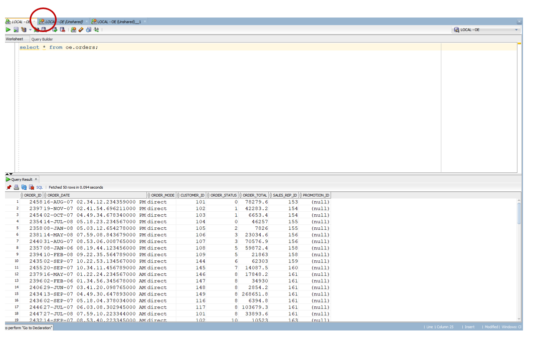
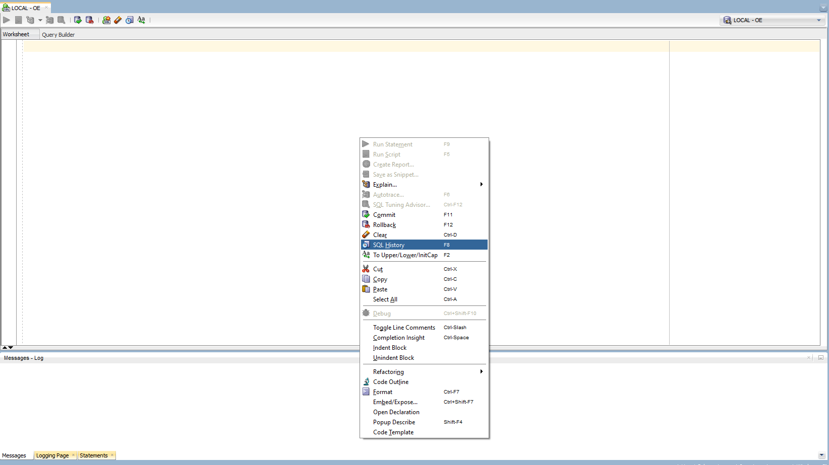
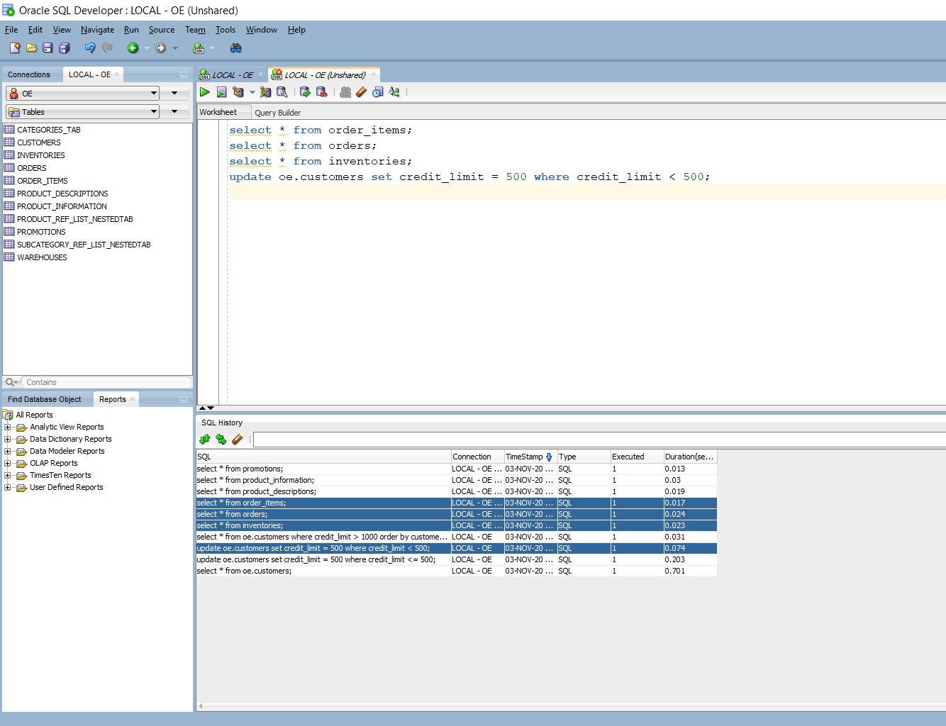
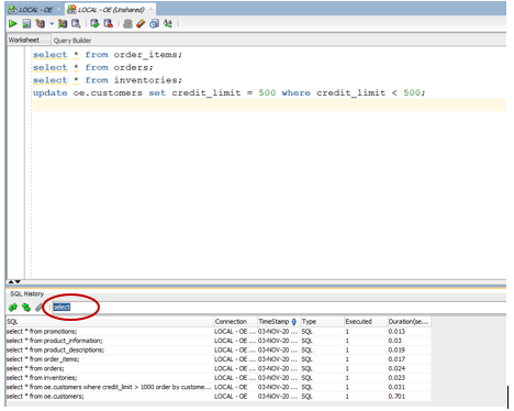
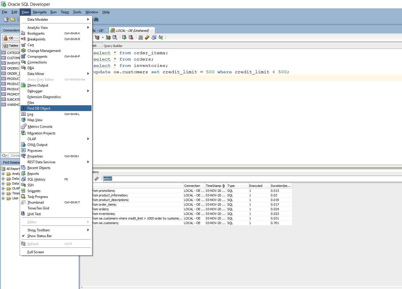
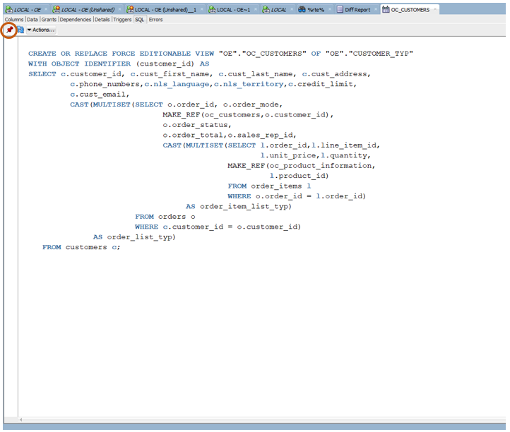
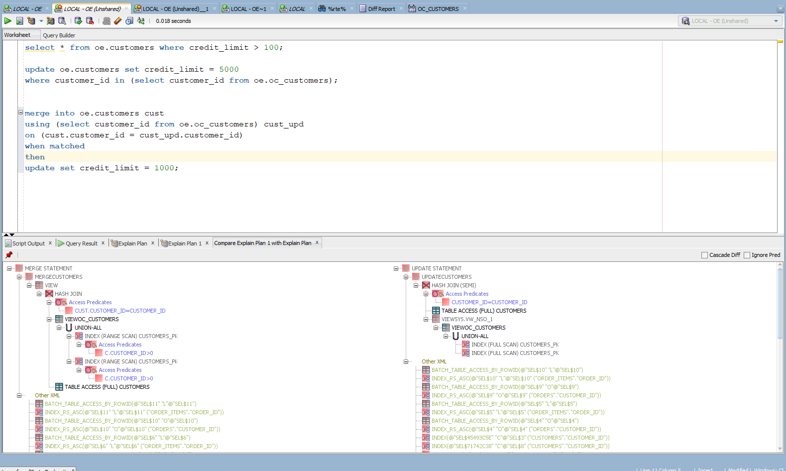
The SQL history opens up at the bottom and now, choose the required SQL statements. Click the to append the selected statements to the existing SQL worksheet. You can highlight multiple SQL statements and copy all of them to the worksheet at once.

The highlighted SQL statements got added to the SQL worksheet in one shot.

There is also a search option with this window. This helps to narrow down the SQL statements based on an object name, SQL functions used, or any other specific detail from the SQL statement. The keyword select is entered in the search box to filter only SQL statements containing select.

Find DB object – Catch me if you can

This search feature is great to perform impact analysis across the database. It helps to identify the dependencies and directly look into the code segment containing the object name or literals or any other search string. Go to View -> Find DB object to open up the window.

You can customize the search by selecting the required schemas, object types, or include/exclude source code. If a search is going to take a long time, it can be run in the background as well; this allows you to work on other items when the search is running.

The various objects using the searched string are shown.

By clicking the line of code from the search results, the respective object opens up. With this, you can quickly look into all the impacted objects and save many clicks in individually opening them through a schema browser.

The trigger INSERT_ORD_LINE opens up after clicking it from the search results, as shown below.

Search results can also be collapsed or expanded at the schema level.

There is a limitation in the output; only up to 500 records are displayed on this search screen. For any extensive searches, one approach would be to break it down into multiple searches restricting into limited schemas.

Database compare – Catch the difference

This option helps to compare two schemas, usually between different databases. Navigate to Tools -> Database Diff to access it. After refreshing the database or post-deployment, you can run this process to ensure the required objects are available or to check if the migration is successful.

After clicking Database Diff, choose the database connections and various other comparison options in Step 1 of 4.

Choose the object types to be compared between the selected schemas in Step 2 of 4.

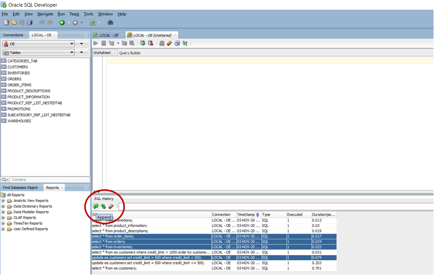
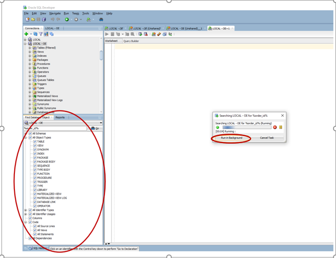
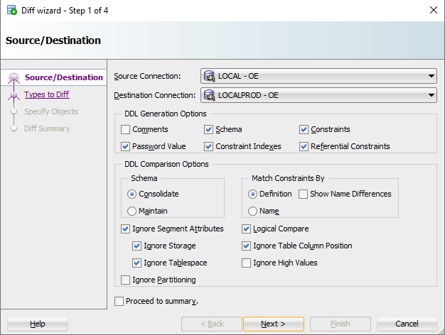
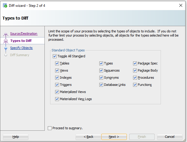
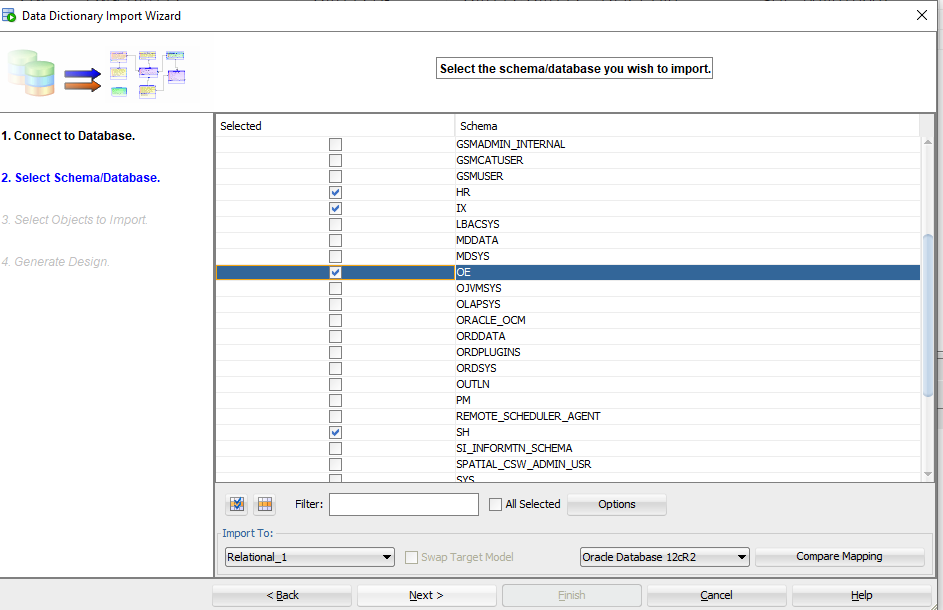
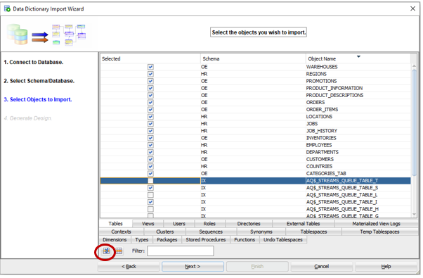
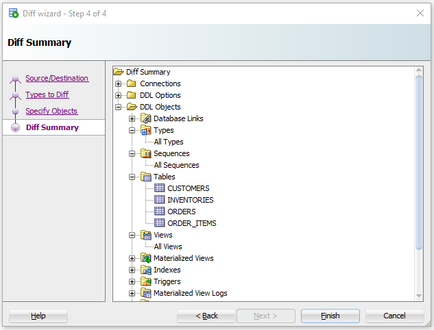
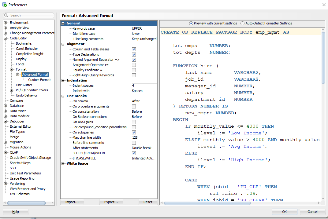
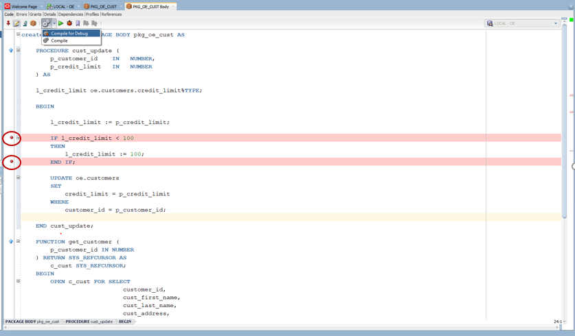
In Step 3 of 4, you have an option to run the comparison for a specific set of objects. To do that, select the schema, type, and click . The list of all items is shown; choose the required ones, click to finalize. To include all objects, just hit Next and move on.

In Step 4 of 4, the summary of the comparison performed is shown. Click Finish to generate the report. As you can see, for tables, only the identified ones from Step 3 are included.

The summary of the comparison is shown below. Any objects available in one schema but not in another is highlighted in green. You can see the details by clicking the item. PKG_OE_CUST is available in the LOCAL_OE Database and not available in LOCAL_PROD database.

Similarly, a warning sign is used to highlight any difference in the objects between the two schemas. Click the item and view the differences.

This process also can be executed in the background to gain some productivity.

Reports – Tell me about everything

SQL Developer contains standard reports which help to quickly browse through the contents and save time compared to manually running the queries required to get those data. This option is available from View -> Reports. This will open a window listing all the available reports

Invalid objects – This report provides a list of all invalid objects and can be run before and after deployments to ensure no new invalid objects are created.

Object Grants report – This provides the overall view of grants assigned to the individual schemas.

Custom reports are also available in SQL Developer under Reports -> User Defined Reports. By right-clicking on User Defined Report and choosing New report, the below screen opens up. You can save any frequently used report or SQL with a report name.

Click on the report name to view the results from the newly created report.

Pinning – Stay where you are

This is a minuscule item but saves many repeated clicks, especially if you are new to SQL Developer. When you open a new object, SQL Developer automatically closes the tab for certain object types. When I open the oe.customers table to view it and then open the oe.oc_inventories table, it closes the oe.customers window. In a way, it helps avoid accumulating a lot of tabs to browse through back and forth. But if you would like to keep the tab open, then it can be pinned.

You can pin the window with the universal icon , and it is always on the top left corner of the window. Any pinned tabs must be manually closed.

In PL SQL packages, procedures, functions, and few other object types, the windows are automatically pinned, which means opening another package does not close the existing package.

Format and Explain Plan – Make it legible

After developing a PL SQL object, the code can be formatted using the format option (ctrl + F7) or right-clicking on the SQL worksheet and choosing Format. The settings related to the format can be controlled in the preferences section (Tools -> Preferences -> Code Editor -> Format). The formatter settings can be auto-detected as well.

A common standard can be created across the team, which would help maintain the same code format and easier maintenance. Selected pieces of code can also be formatted by highlighting only the required portion and formatting it.

The explain plan option helps evaluate the cost and the sequence of operations performed in the SQL statement. This is available from the SQL worksheet and can be viewed by hitting the F10 key or right-clicking and choosing Explain Plan. The cost and cardinality for the SQL statement are shown.

Two different explain plans can be compared to see the difference in steps. Usually, this is done when tuning queries to look for any improvements. Generate the explain plan for the first statement and remember to pin it.

Now, generate for the next statement and right-click on the second explain plan tab to compare with the first one. This helps to compare the plans side by side.

Debugging – A blessing for every developer

SQL Developer has a debugging feature for the PL SQL programs. A specific procedure, function, or package can be debugged with breakpoints, and the value of the variables can be observed during the execution. To set a breakpoint, click on the desired line of code on its left side and compile it with the debug option.

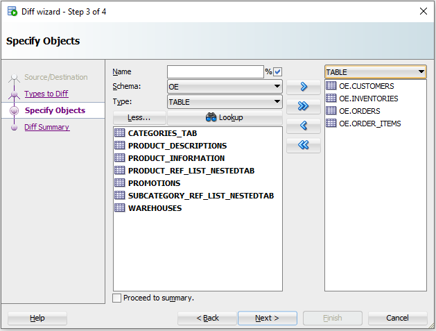
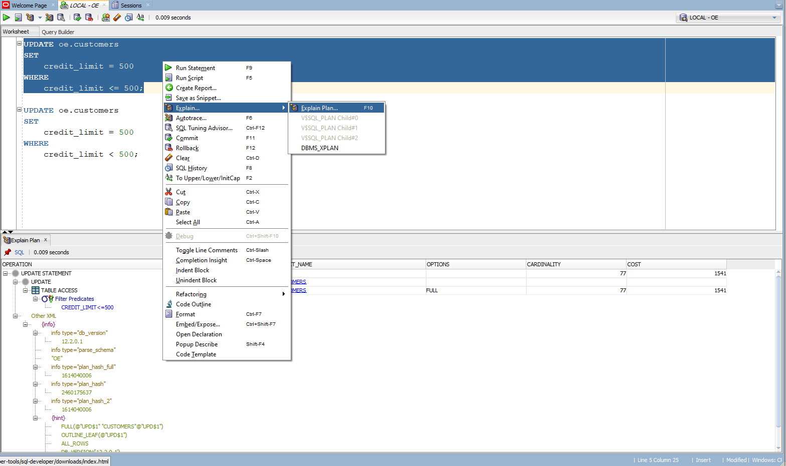
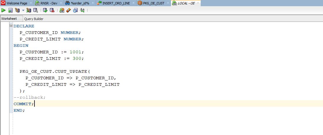
Click the icon to start the debug process. The input values to be provided during execution can be keyed in the parameters section. The program gets executed after clicking OK. I have provided an input value of 1001 to p_customer_id and 50 to p_credit_limit.

Now, the process has stopped at the breakpoint. Here, a whole range of operations can be performed. Under the Data tab, the values of the variables can be observed as the process gets executed. With the icons on the top, the debugging process can be stopped, resumed, moved into another subprogram, etc.

Under the Data tab, you can observe that l_credit_limit is set to 50 before entering the IF clause.

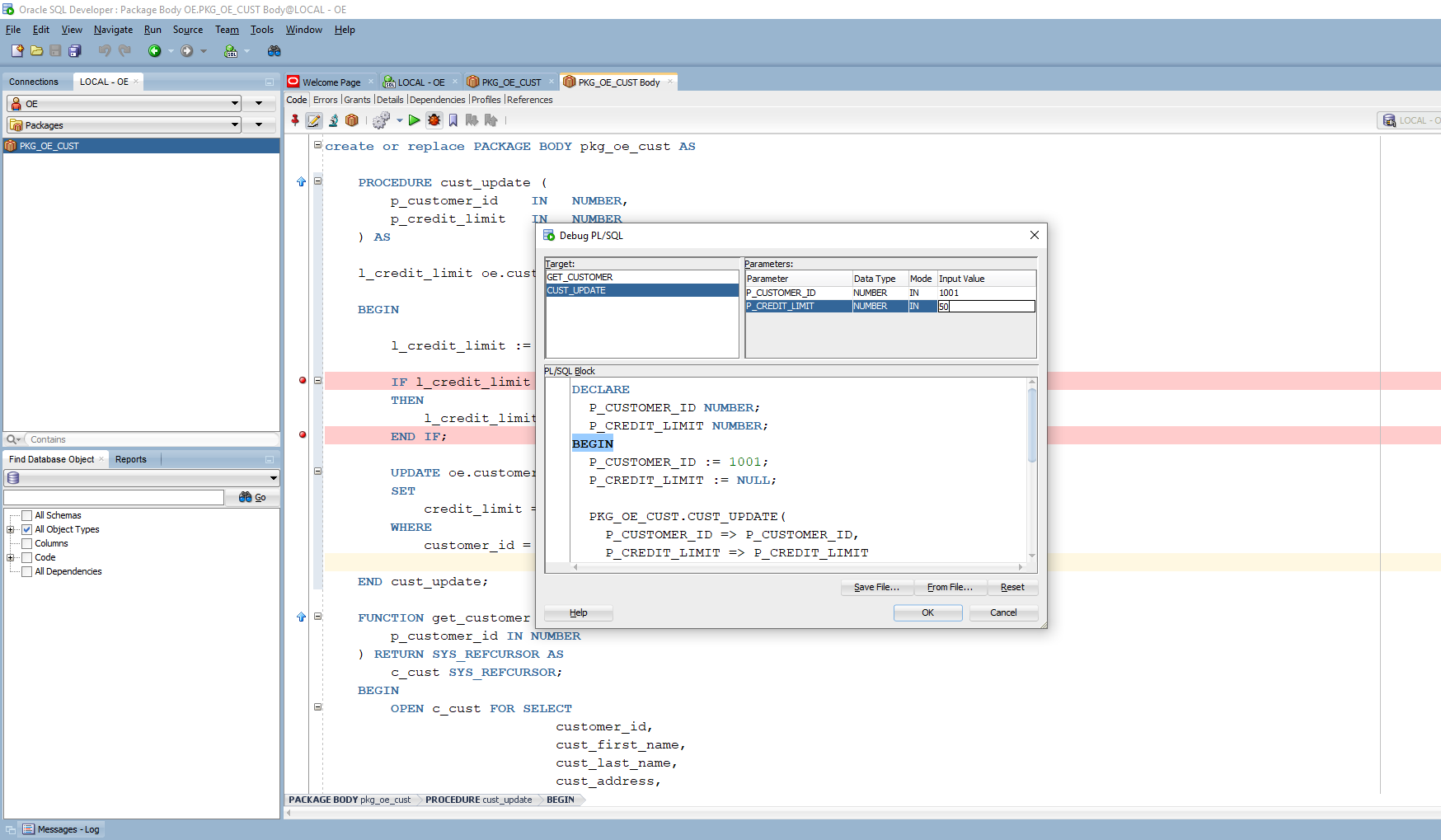
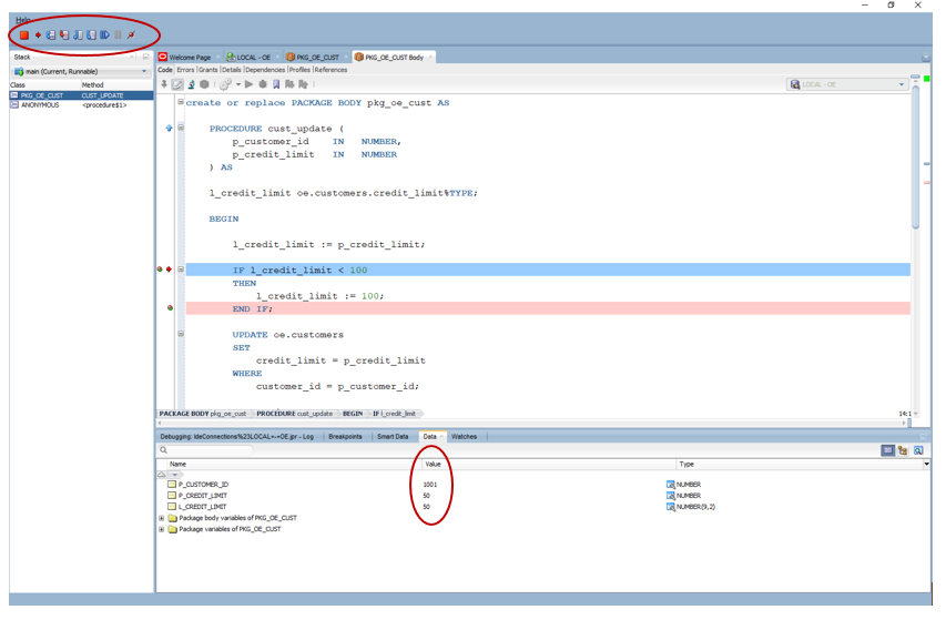
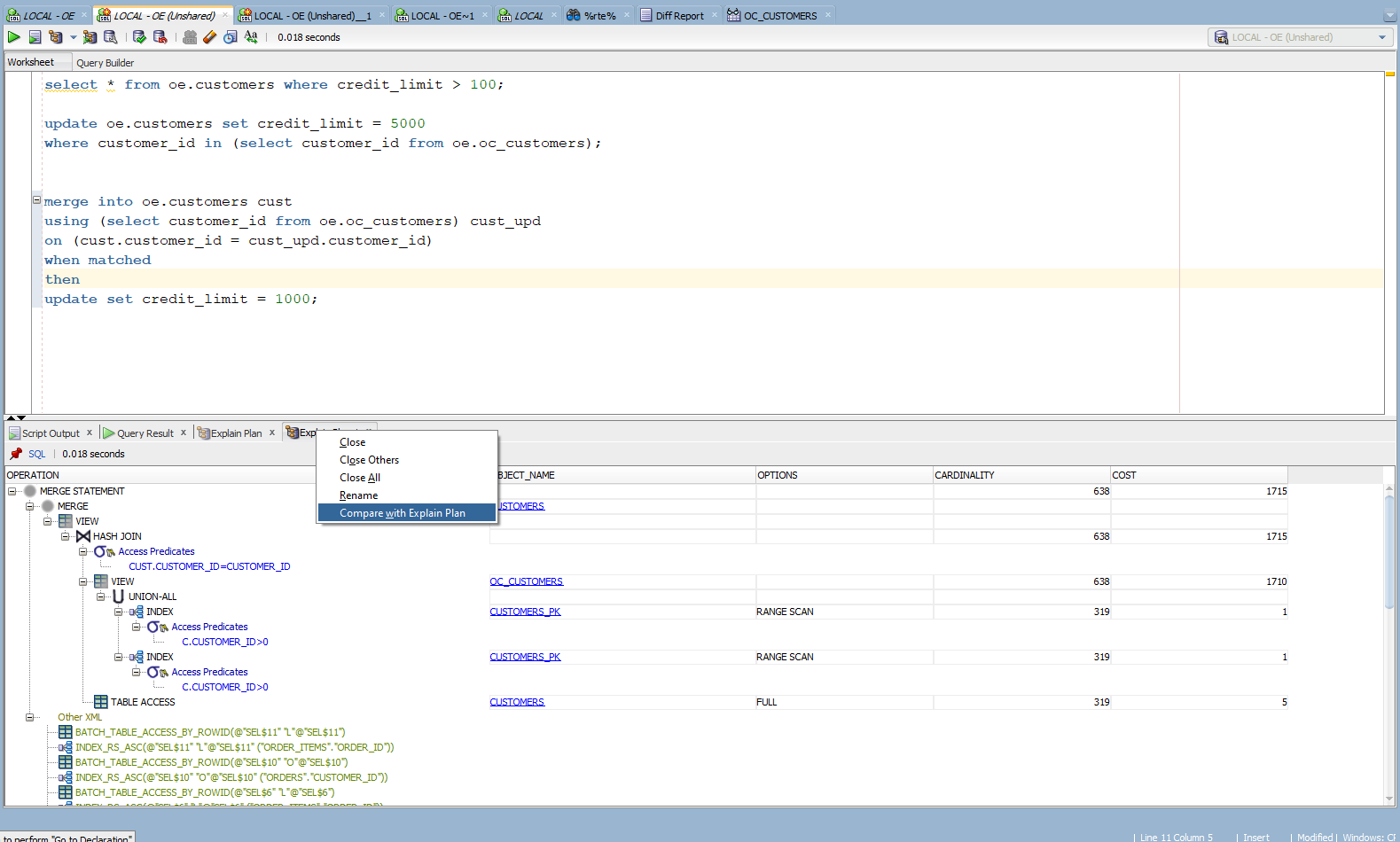
After hitting or F9 to resume, the process stops at the next breakpoint. Here, you can observe, the l_credit_limit value is updated to 100.

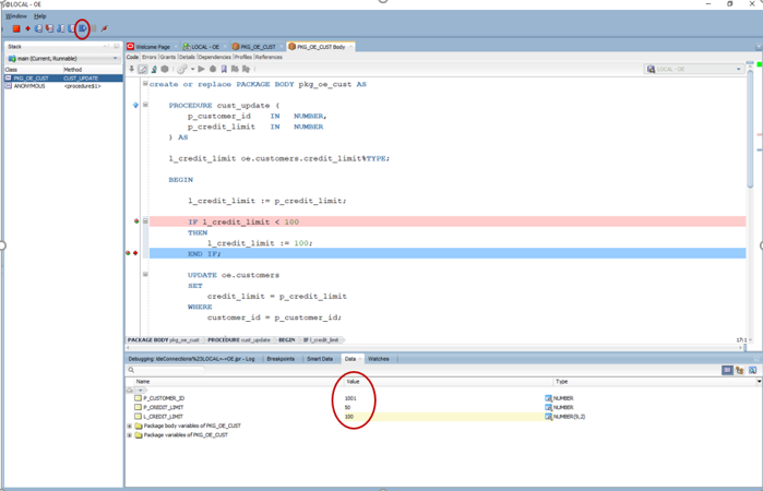
Hitting or F9 to resume will complete the execution of the cust_update procedure, as there are no more breakpoints.

If there are output cursors returned as part of a function, the cursors’ dataset can be viewed as well. The procedure get_customers returns a cursor to view the customer details for an input customer. The process is executed by clicking , entering 1000 for p_customer_id under the parameters section, and clicking OK.

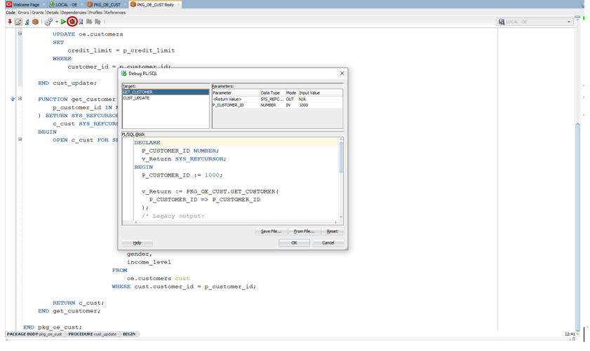
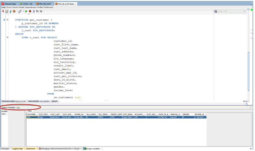
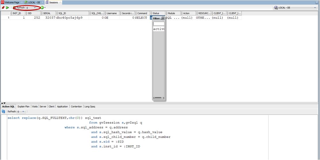
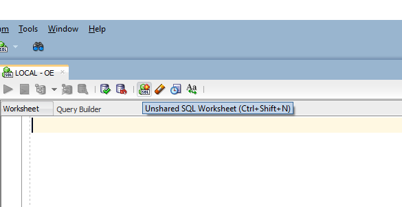
After running the function, the cursor’s output value is shown under the Output Variables – Log section.

In some instances, the code block to execute the procedure or function can be copied to a SQL worksheet and executed from there. This helps to quickly set up the parameters when running these processes from a worksheet. The p_customer_id is set to 1001 and p_credit_limit to 300. This process can be executed several times for different values directly from this SQL worksheet by clicking on the top left.

Sessions monitor – What’s going on

The sessions monitor screen identifies the active sessions currently executed in the database with details like SQL Id, SID, execution time, OS user, client identifier, and many others. It can be opened up from Tools -> Monitor Sessions. If you have any long-running processes, those can be identified here and you can monitor the batch processes.

There is a refresh timer at the top, which can be set for an automatic refresh of the screen. Filters can be applied at the top of each column to look for sessions only under a particular schema, specific OS user, or only active sessions.

It would be hard to capture any process which takes less than a few seconds here, and a better approach would always be creating debug logs for such processes. In the case of SQL statements with bind variables, this does not show the bind values; rather only displays them as bind variables.

The wait tab at the bottom shows any session waits caused due to object locks or resource availability. The Active SQL tab displays the exact statement currently executed by the process, and the Explain Plan tab shows the cost associated with the statement and execution plan.

These features help to quickly get a grasp of the current processes executed in the database.

Database Design diagram – A must-have artifact

A data model diagram of the database assists in understanding the relationships between the objects. The option is available under File -> Data Modeler -> Import -> Data Dictionary. After choosing the connection to log in, the list of schemas can be selected.

Following that would be a screen to select tables, views, and any other objects. After choosing those, hit finish. To select all the tables, use the check all icon at the bottom left.

The data model diagram showing the relationships between the objects and keys, indices, and many other details is provided. These details are entirely customizable, and the diagram can be saved as a PDF or Image file by right-clicking and choosing Print Diagram -> To image file / To PDF file.

This is one of the essential artifacts maintained for the database, and it also helps to perform the impact analysis at a high level.

Get the most from SQL Developer

Just like any other tool, you get used to this and discovery new functionality as you start working in it. The tool is easy to set it up and does not require the Oracle client to be installed. There are a lot more features and utilities available in this tool apart from the items discussed here. Give SQL Developer a try and improve your skills.

Use the links below to download the SQL Developer and the documentation to explore further.

https://www.oracle.com/tools/downloads/sqldev-downloads.html

https://docs.oracle.com/en/database/oracle/sql-developer/20.2/books.html

 

The post SQL Developer – A great tool and better ways to use it appeared first on Simple Talk.

from Simple Talk https://ift.tt/3nG4Sti
via