Monday, March 29, 2021

Data Platform: Links to Study and Learn

Last Friday I appeared in the middle of a Brazilian Twitch live made by a friend and while they were talking and studying, I provided some links full of content to them.

Nowadays, there are a lot of free content on internet. Not only free content, but also content well organized in a good sequence for learning.

So, to help everyone find this content, my idea was to start this blog post that hopefully will stay alive with all the comments and suggestions of new links from all of you, my 2 readers (hi, mom !).

Learning

30 Days to Learn It

This is a very recent and interesting project. You are challenge to complete learning tracks in 30 days and if you manage to do so, you receive a big discount on the certification exams.

Microsoft Learn

Here you can find even additional learning tracks besides the ones available on the “30 days to Learn It”. This site concentrates all the Microsoft Learning content.

SQL Server Workshops

Here you can find very interesting workshops about SQL Server and Azure SQL. For example, the best workshop about SQL Server Big Data Cluster is on this link.

The link uses GitHub features to host the explanation and steps and link back to Microsoft documentations to be sure the workshops will be always updated.

Microsoft Learn Blog

One very important reason to always take a look on this blog is the announcement of Beta Exams. When Microsoft is about to release a new certification exam, they first test the certification in the real world, inviting some people to take the exam almost for free. It’s not totally free to ensure people will not book and fail to attend the exam.

Beta exams have 80% of discount and you receive a voucher of 20% to be used on your next Microsoft exam.

RedGate Free E-Books

Free e-books are always good to learn and RedGate provides many of them.

Communities

Data Saturdays

After PASS death, the community built a replacement for the SQL Saturdays: The Data Saturdays. They are working very well.

Azure Data Community

This is the new Data Community built by Microsoft to keep all Data User Groups together. The community already includes 107 user groups. On this new world where all conferences are made online, why not register for all of them?

Microsoft TechCommunity

This is a very complete Microsoft Community site focused in forums and Q&A for all Microsoft products, but also with many technical publications available

Blogs

I’m not a great blog follower, I prefer to follow people on twitter and choose the blogs according to the publications, but there are some blogs we can’t miss. Probably you know many more, tell us on the comments

You can also take a look on the blog recommendations on the Azure Data Community

Twitter

Following the right accounts on Twitter can bring to you the most important news in first hand. Microsoft has twitter accounts for each product groups.

Microsoft on Twitter

Azure Purview Azure Data Explorer Azure Synapse Analytics Azure Monitor Azure Weekly Azure SQL DB Azure Data Studio Azure Data Factory Azure SQL Microsoft SQL Server Power BI 

Additional Microsoft Related

Data Science

More Twitter Accounts

A good way to find interesting accounts is to take a look on the conversations with the accounts you are already following. You will discover other accounts interacting with these ones and with related interests

Conclusion

The amount of information available for free on the internet is huge. If we manage to get it in an organized way, we not only will learn what we need for free, but we may achieve a level of knowledge way deeper and up-to-date than other regular training methods.

However, everything changes so fast a blog like this one needs to be alive, always being updated with suggestions from everyone, to continue to be relevant.


The post Data Platform: Links to Study and Learn appeared first on Simple Talk.


from Simple Talk https://ift.tt/39H5Zoj
via

Friday, March 26, 2021

Oracle sequences: The basics

Many database applications make use of “meaningless ids” or “synthetic keys” rather than using columns of user data to construct the primary key for their tables. For a very long time, the Oracle RDBMS has supplied the “sequence” mechanism to generate such values efficiently and with minimum contention between transactions. Despite a history of several decades, sequences are often misunderstood and misused – and there are a few threats involving sequences that Oracle Corp. is still working to minimize.

In this short series of articles, I aim to eliminate the most typical misunderstandings, warn you of the threats and provide ideas for workarounds. I’ll start by discussing the pre-12c use of sequences for single-instance, Oracle, then I’ll move on to the critical changes that are relevant to multi-instance RAC, and end with some comments on the features that appeared more recently in 12.1, 18c and 19c to deal particularly with “Application Continuity”, RAC and “Sharding”.

Defining a sequence

Until 12c, the full syntax of the create sequence command is as follows:

CREATE SEQUENCE [schema_name.]{sequence_name}
        START WITH      n
        INCREMENT BY    n
        [MINVALUE n | NOMINVALUE ]
        [MAXVALUE n | NOMAXVALUE ]
        [CACHE n | NOCACHE]
        [ORDER | NOORDER]
        [CYCLE | NOCYCLE]

The shortest statement you could use to create a sequence, however, would be simply:

CREATE SEQUENCE sequence_name;

This command would be equivalent to:

CREATE SEQUENCE sequence_name
        START WITH      1
        INCREMENT BY    1
        MINVALUE        1
        NOMAXVALUE -- which is effectively 1e28 - 1
        CACHE           20    -- which is usually a bad idea, as we shall see later
        NOORDER
        NOCYCLE

Oracle invented sequences to make it possible to supply on demand a (virtually) limitless sequence of numbers that were guaranteed to be unique. The easiest way to do this is simply to keep a globally visible counter and increment it every time a session says: “give me a number” (or, more accurately, “tell me the value of sequence_name.nextval”).

But Oracle has to keep track of the last number supplied to avoid the risk of supplying the same number twice – that’s easy enough for a database system: just keep the most recent number in a table. However, that makes things very slow if you have to update a table each time someone needs the next number. You ought to use an autonomous transaction so that nobody has to wait for the first session to commit its current transaction before the next number can be generated. Therefore, Oracle uses recursive, autonomous transactions to handle the table updates, and it avoids updating the table for every single call to nextval by counting in memory and remembering when it will next need to update the table. Unfortunately, Oracle refers to this “in-memory” mechanism as the cache – which is very misleading.

A common strategy for “home-made” sequences is to have rows in a table with columns (sequence name, most recently used sequence number), then write a function that selects the relevant row from the table for update, increments the number, updates the table, and supplies the number to the end-user. Behind the scenes, this is exactly what the Oracle software does, though being an internalized mechanism, it can “cheat” in ways that the home-grown code can’t.

You can see the database image of a sequence by querying the view user_sequences. Assuming I’ve just created a sequence called s1, here’s a suitable query followed by the result it gives me immediately after I created the sequence, followed by the result I get after one call to fetch s1.nextval:

select
        min_value, max_value, 
        increment_by, cache_size, last_number, 
        cycle_flag, order_flag
from 
        user_sequences
where 
        sequence_name = 'S1'
/

If you have DBA privileges, you could go one step further by finding the object_id of the sequence and then querying the dictionary table (seq$) that the view is based on. Again, I’ve run the query twice, once before and once just after the first call to s1.nextval):

select 
        minvalue, maxvalue, increment$, cache, highwater, cycle#, order$ 
from 
        seq$ 
where
        obj# = 124874
;

There’s one final option for checking the state of a sequence – the in-memory information that is visible to privileged accounts through the dynamic performance view v$_sequences (the unexpected underscore isn’t a typo). In this case, I’ve queried the view just once, after the first call to s1.nextval (the sequence won’t even be in the view until the first call to nextval), and I’ve included a column that isn’t available in the dictionary table:

select
        min_value, max_value,
        increment_by, cache_size, highwater,
        cycle_flag, order_flag, nextvalue
from
        v$_sequences
where
        object# = 124874
/


As you can see, the dynamic performance view has a column nextvalue that holds the value which will be supplied the next time a user calls for s1.nextval.

All three views hold a “highwater” value (though it’s called last_number in view user_sequences). When a call to s1.nextval returns the value shown in highwater (highwater and nextvalue are the same), the session making the call will execute and commit a recursive transaction to add the increment value to the current highwater and update the seq$ table.

The “cache” isn’t a cache in the traditional sense, it’s just a single pair of numbers (no matter how large you set the sequence cache size): the current value and the value at which you bump the highwater value. There is no resource penalty for setting a large cache for a sequence, and the most important fact about sequences is that, in most cases, you should probably be using a large cache size.

Performance issues (Single Instance)

As I said at the start of this article, the commonest use of sequences is to generate synthetic keys. If you’ve used a sequence in this way for a table that’s subject to a high volume of activity – and particularly if it’s subject to highly concurrent activity – you want the sequence numbers to be supplied as quickly as possible. You don’t want to have to pause on every 20th call for a data dictionary table to be updated, and you don’t want to wait because 50 other sessions are all colliding on the same sequence maintenance.

Cache size

It’s quite easy to recognize this issue in single-instance Oracle as you’ll see sessions in v$lock waiting on the SQ enqueue (lock) in mode 4, and the reported wait event will be enq: SQ - contention, with p1 set to the object_id of the sequence they’re waiting for. The solution to this problem is simply to increase the cache size, and it’s not uncommon on very busy systems to see sequences with caches in the thousands:

alter sequence s1 cache 10000;

Given that it’s often important for performance and concurrency to increase the cache size of a sequence from the default 20, you should appreciate that it’s a bad idea to create a single sequence to supply values for every single column that needs unique meaningless values. Play safe – give each synthetic key its own sequence. (Some other RDBMS do this automatically through an “identity” data type, but that feature has been introduced only in recent versions of Oracle.)

This default performance problem is sometimes made worse by a demand from the end-users that “there should be no missing numbers” which leads to DBAs setting the sequence to nocache. In other words, every call to nextval results in the highwater being incremented and the seq$ table being updated. This can be a massive source of contention and could easily end up as the key bottleneck in the system – and to make things worse, it doesn’t stop numbers from going missing (e.g. a session might have to rollback or might crash after its call to nextval, and the value would then be lost).

Oracle sequences are not intended to provide an unbroken sequence of values; they are only intended to supply a unique set of numbers. If you need some form of sequential audit trail (and you want it to be scalable) then you will have to do some fairly careful coding to create your own – it’s not a trivial exercise.

Index Contention

There is another common performance issue that is a byproduct of using sequences to generate unique ids: if uniqueness is important, you ought to declare a constraint on the relevant column, and a unique (or primary key) constraint will automatically result in Oracle creating a corresponding index. The index will become a point of contention because all the sessions that are trying to insert a new row will have generated sequence numbers which are (a) very close to each other and (b) the highest values generated so far; this means you will have multiple sessions trying to insert new values into the same (so-called “right-hand”) leaf block of the index.

In these circumstances, you’re likely to see a lot of waits for “buffer busy wait” on the index; you may also see waits for “enq: TX – index contention”, and even “enq: TX – allocate ITL entry” as sessions queue up waiting for an index leaf block split to complete. Unfortunately, there’s no good solution to this problem, though there are damage limitation mechanisms you could implement, and one of the enhancements Oracle 18c supplies is a declarative version of one of the commoner mechanisms.

Once upon a time, a common suggestion to avoid the index hot-spot was to recreate the index as a “reverse-key” index but, for continuously growing tables, that’s a bad idea as it typically replaces a few seconds of “buffer busy wait” with minutes (or more) of extra “db file sequential read” waits. (For an explanation of this comment, see: https://jonathanlewis.wordpress.com/2015/06/17/reverse-key-2/ )

If you’re licensed for the partitioning option, a better way to remove the hot spot is to recreate the index as a globally hash partitioned index – with the usual proviso that the number of partitions should be a power of 2 to ensure equal sized partitions. There are some optimizer-related drawbacks to partitioning an index in this way, but since we’re talking about the use of sequences for synthetic (meaningless) keys, the only queries you expect to see targeting the index are likely to be of the form: unique_key = {constant}, and the optimizer is unlikely to be misled by a query with a predicate of that type.

The partitioning option is expensive, of course, and isn’t available on Standard Edition, so the manually coded fall back is spread the hot spot by manipulating the sequence number after you’ve fetched it. First, you have to pick a number that is so large that you think the sequence will never need to reach it (say 1e10). Then you add a session-dependent value to the sequence number that makes sequence values that are close to each other end up widely separated in the index because they were inserted by different sessions. For example, you might add (1 + mod(sid, 16)) * 1e10 to the sequence value; this will give you most of the performance benefit of hash partitioning your index into 16 partitions – splitting your one hot-spot into 16 “slightly-warm” spots.

Inevitably there’s a price to pay for this scaling mechanism. In an ideal world, an index on data generated by a sequence would use close to 100% of the available space in each index leaf block because Oracle would be doing what it calls “leaf node 90-10 splits” each time the right-hand (high value) leaf block split. If you spread the inserts across N different insertion points in the index (using 1+mod(sid,N) as above), then all but the highest insertion point would be doing “50-50” leaf node splits.

Although Oracle has a statistic in the instance and session activity statistics (v$sysstat / v$sesstat) for “leaf node 90-10 splits”, a better name would be “leaf node 100-0 splits”. The “split” simply adds a leaf block at the right-hand (high-value) end of the index and carries on into it; it doesn’t copy any data from the preceding leaf block. By comparison, the “normal” mid-index leaf node split links a new leaf block into the right place then moves roughly half the data from the existing leaf block into the new leaf block.

The side effect of manually “pseudo-partitioning” an index in this way is that it might operate at roughly twice its previous size. (And that’s not allowing for the fact that you now have an index where the smallest entry is a few bytes longer than the largest entry used to be.) In real-life, there are a couple of odd concurrency effects that can make any index with hot spots waste a significant amount of space, so the change may not be quite as dramatic as the theory predicts.

Miscellaneous

I’ll finish this article with a brief round-up of the remaining, less commonly used features of the pre-12c sequence.

Start with: you can specify any legal integer value as the first value to use, positive or negative; the default is 1.

Increment by: although I’ve been discussing sequences that increase by 1, you can set the increment to any legal integer value (positive or negative). So if you wanted a sequence of the positive even numbers you could specify “start with 2 increment by 2”. The default increment is 1.

Minvalue: if your increment is negative, you can set a value below which Oracle raises an error (ORA-08004: sequence goes below MINVALUE).

Maxvalue: the mirror to minvalue – with a positive increment in place you can set a value above which Oracle will raise the error (ORA-08004: sequence goes above MAXVALUE).

Cycle: I don’t think I’ve ever seen this used in the wild, but you can set up a sequence to repeat if it has a maxvalue with positive increment or a minvalue with negative increment. If the call to nextval would push the sequence past its min/max value then it goes back to its start value and continues from there.

Order: This is an option that applies very specifically to how RAC handles sequences, and I’ll leave that to the second article in the series.

If you start playing around with sequences, you’ll discover that there are a number of ways of combining the options to produce fairly self-explanatory Oracle errors. For example:

SQL> create sequence s4 start with 10 increment by 15 nomaxvalue cycle;
create sequence s4 start with 10 increment by 15 nomaxvalue cycle
*

There are so many possibilities that there’s no point in trying to list all of them. If you want to read the Oracle error messages file ($ORACLE_HOME/rdbms/mesg/oraus.msg) then the error numbers relating to creating sequences go from ORA-04001 to ORA-04016.

Summary

In this first article, I’ve described the basic and most common use of sequences and highlighted the need to choose a sensible cache size to avoid concurrency problems with the sequence itself. In particular, I’ve emphasized the threat of defining a sequence as nocache while pointing out that, contrary to popular assumption, this option doesn’t stop you “losing” sequence numbers.

I’ve pointed out the concurrency issues that arise when you create an index to enforce the uniqueness of sequence values, and discussed strategies for minimizing the threat, at the same time pointing out that whatever you do there are side effects. In passing, I’ve mentioned that time-based indexes will exhibit similar behaviour to sequence-based indexes.

Finally, I’ve given you a brief run-down on the less frequently used options for defining a sequence, leaving any comments about the order option to the next article, which will start talking about RAC and the extra care needed when handling sequences in a multi-instance system.


The post Oracle sequences: The basics appeared first on Simple Talk.


from Simple Talk https://ift.tt/2Pe08Q1
via

Load/stress testing .NET apps with Apache JMeter

You created a brand-new API developed on the REST principles and set up under the ASP.NET world. Now you want to test it. More specifically, you want to create and run some stress tests for your API in to understand how fast it is and how much load it supports.

The .NET team has discontinued their cloud-based load testing service a while ago under Visual Studio 2019 due to the lack of community adoption. Users in the community now had to think about the one million-dollar question: What is the best load/stress testing tool for my .NET projects? The answer starts right before the “.NET projects” part. Most people load testing nowadays are doing that against web APIs or, at least, web applications (that handle endpoints the same way with different media types).

Because of this particular point, these types of tools are mostly agnostic because some of them provide very platform-specific features like the JSR223 (a scripting language for Java apps) assertions that JMeter supplies, for example.

In this article, you’re going to dive into the universe of Apache JMeter, one of the most used agnostic load test tools in the software development community by testing it against a REST application created in ASP.NET.

JMeter setup

JMeter is made with Java 8+, so it requires the JDK (Java Developers Kit) on your machine before using it. Be sure to download and install it. The installation for JMeter is a little bit different from the usual installer approach. Instead, you must go to the JMeter Download page and download the binary zipped file.

Unzip it and navigate to the bin folder in which you will find a file called jmeter.bat. Double-click it and the window shown in Figure 1 will show up.

Figure 1. Starting up Apache JMeter tool

The GUI tool is going to load in the background until it pops up as shown in Figure 2.

Figure 2. Apache JMeter initial screen

Take some time to look at the options and menus displayed on this screen.

The .NET application

For simplicity, this example will not create an API application from scratch since it’s not the focus of the article. You can test whatever web application or live API on the web that you have handy. However, to get the feeling of local tests, use a CRUD API I’ve developed before in another article: Creating ASP.NET Apps with React.

You may find the source code here. Please, clone it to your machine, cd into the \ReactASPNET\ReactASPCrud\ReactASPCrud\ folder, and run the following command:

dotnet run

This command will start up the application at http://localhost:5000. Leave it there and get back to the tests.

JMeter test plans

In JMeter, everything starts from a Test Plan. That’s the very definition of how JMeter groups things together as a composition of runnable tests. You can have as many test plans as you want for a single project.

JMeter loves groupings. Typically, since you’re dealing with stress testing, you have to deal with loops. Loops are used to check if the given resource can handle all the concurrent load that you’d eventually have in a real-world scenario. That’s why you always start by adding a new Thread Group to your Test Plan. Figure 3 demonstrates the menus you may access to add a Thread Group.

Figure 3. Adding a new Thread Group to your Test Plan

You may see a bunch of fields under the Thread Properties section. Among all these fields, there are three of them that are more important:

  • Number of threads (users): as the name suggests, this field represents how many users you envision to be using the same endpoint at the same time. Usually, you’re going to add a value way higher than the average of concurrent users you have in order to stress your system.
  • Ramp-up period (seconds): this field considers a ramp-up strategy over time which tells JMeter how long to wait until loading the next user (request).
  • Loop count: how many iterations this thread group test may have?

Figure 4. Configuring the Thread Properties of your Thread Group

Great! Now that you have your Thread Group set up, you need to determine what this group will iterate over. You can iterate over many different types of requests, such as JDBC, JMS, FTP, etc. However, since you’re dealing with a REST API, the HTTP requests are the next elements to configure.

But first, take a shortcut through a very nice config called HTTP Request Defaults. Figure 5 shows how to access this option.

Figure 5. Adding a new HTTP Request Defaults

This option helps you globally configure HTTP properties that are most commonly used such as the URL root address of your API, HTTP Authentication settings, IP, port, etc. This is a great option when you have to test many API endpoints within the same Thread Group without having to explicitly duplicate the information.

Go ahead and fill in the options as shown in Figure 6.

Figure 6. Setting up HTTP Request Defaults options

You may also notice that these configs are being stacked on top of each other on the left panel of the JMeter GUI tool. It stacks things in a nested way in order to keep the hierarchy of your settings, so pay attention to that.

Now that you have a default configuration for your HTTP requests, move on to add the first API endpoint to test. Start with the most simple one: the users’ listing at https://localhost:5000/api/users.

Figure 7 shows how to add a new HTTP Request Sampler element.

Figure 7. Adding a new HTTP Request to the Thread Group

Figure 8 demonstrates how you may fill in the fields. Remember that the Server Name/IP and Port Number were already provided within the previous Defaults setting, so there’s no need to set it again.

Figure 8. Setting the HTTP Request endpoint details

This is basically everything you need as a minimum setup for an HTTP request suite. However, in order for you to check the results of the stress test, you need to ask JMeter to measure the right metrics. JMeter can deal with a bunch of different and useful result listeners. Take a look at the two most used ones.

Figure 9 and 10 shows how to add a new Summary Report and a new Graph Results listeners, respectively. Go ahead and do that to your Test Plan as well.

Figure 9. Adding a new Summary Report to the Test Plan

Figure 10. Adding a new Graph Results to the Test Plan

There’s no better way to see what these two listeners can rather than run the Test Plan. Before that, make sure to save your current test settings by hitting Ctrl+S on the keyboard. It’ll trigger a new window (Figure 11) for you to select the directory to save the tests as a file with a .jmx extension.

Figure 11. Saving the current test suite

You can then add this file to your project repository, and other members of your team can load it on their own JMeter tools as well.

Now, click the Start button on the top bar or hit the Ctrl+R keyboard shortcut to execute the Test Plan. As the logs start to show up on the terminal window where you started the local API application, you’ll get to see the summary of the execution when you click the Summary Report item on the left panel. That’ll display the screen shown in Figure 12.

Figure 12. Displaying the Summary Report whilst running the tests

That is useful information since you can see not only the number of samples running at the time but also the average of users, the maximum number of samples at any time during the execution, the error rate, and more.

If you open the Graph Results item, that may show similar results as in Figure 13.

Figure 13. Animated results from the Graph Results whilst running the tests

This graph not only brings important information about the number of executed samples, but also graphically displays the throughput vs the deviation of the tests. The higher the throughput, the more the application can deal with heavy loads of requests. The opposite is true for the deviation. In this example, the average was around 650 requests/minute.

Extra listeners

There are a couple more nice listeners to consider when developing your JMeter tests. Take some time to explore them as well. The first one is the View Results Tree. You can add it the same way you added the previous ones, via Add > Listener > View Results Tree.

Before you rerun the tests, make sure to clean up the previous execution. You can do that by clicking the “gear and two brooms” icon on the top bar. Then, rerun the tests. You may see a similar result to the one shown in Figure 14.

Figure 14. Displaying the View Results Tree results

Here, JMeter is going very granular by displaying each one of the request’s information as well as HTTP headers, body size, response code and message, and many more. This is great when you need to search for a very explicit error in specific scenarios.

Another significant measure can be displayed by the Response Time Graph as shown in Figure 15. It works by plotting a graph with two axes: the time vs the number of requests. This graph shows the request/response throughput through the time execution.

Figure 15. Displaying the Response Time Graph results

Again, you can add this type of listener via the same steps as before.

Response assertions

During the tests, it is common to have scenarios where you’d like to check for a specific HTTP response status or even if the response body attends to a specific condition. For situations like that, JMeter provides you with the Assertions. Start with the HTTP response status assertion configuration.

Figure 16 shows how to add a new one to your Thread Group.

Figure 16. Adding a new Response Assertion checker

Make sure to check the Response Code option in the Field to Test config. The Pattern Matching Results must be set as Equals as shown in Figure 17.

To add a new pattern click the Add button on the bottom side of the screen and add the 200 as the value for the Patterns to Test option.

Figure 17. Setting up the Response Assertion

That’s it! Whenever you receive an HTTP status code other than 200 the View Results Tree listener will show the error.

Another interesting assertion available for APIs that make extensive use of JSON is the JSON Assertion. To add it, go to the same menu Add > Assertion > JSON Assertion and configure it as shown in Figure 18.

Figure 18. Setting up the JSON Assertion

The Assert JSON Path exists field receives an expression to catch a specific value from the JSON response.

Listing 1 shows an example of the users’ list currently returned by the API. Since the data is always randomly generated at start-up, your test would fail. Make use of this to test the failing assertion. The JSON Assertion states that JMeter must check if the name property of the first list item is equal to “Susan MacDonald”. Don’t forget to check the Additionally assert value checkbox.

Listing 1. JSON response from the users API

[
   {
      "id":1,
      "name":"Mary Gay",
      "email":"mary@yahoo.com",
      "document":"0562264851",
      "phone":"+1 888-452-1232"
   },
   {
      "id":2,
      "name":"Neil Strip",
      "email":"neil@outlook.com",
      "document":"-654353851",
      "phone":"+1 888-452-1232"
   },
   {
      "id":3,
      "name":"Jonathan O'Neil",
      "email":"jonathan@outlook.com",
      "document":"0424625040",
      "phone":"+1 888-452-1232"
   },
   {
      "id":4,
      "name":"Joe Spenser",
      "email":"joe@outlook.com",
      "document":"1415116364",
      "phone":"+1 888-452-1232"
   },
   {
      "id":5,
      "name":"Jonathan O'Neil",
      "email":"jonathan@hotmail.com",
      "document":"-367589335",
      "phone":"+1 888-452-1232"
   }
]

Figure 19 shows the View Results Tree execution results.

Figure 19. Displaying the wrong JSON assertion results

As you can see, the assertion failed because the expected value doesn’t match the received one, which is “Mary Gay”.

If you update the JSON Assertion accordingly, then your tests will pass.

Load/stress testing .NET apps with JMeter

As you’ve seen, JMeter is a powerful tool that comes with many built-in functionalities for various scenarios. Apart from that, JMeter’s community provides you with an enormous amount of open-source plugins that you can add to give even more flexibility and power to your load tests. One of them that is very useful is the JSONFormatter that helps with beautifying your HTTP JSON responses.

Last but not least, make sure to refer to its official docs for more on what it is capable of doing.


The post Load/stress testing .NET apps with Apache JMeter appeared first on Simple Talk.


from Simple Talk https://ift.tt/31m5j2R
via

A data transformation problem in SQL and Scala: Dovetailing declarative solutions Part II

Part II : Equivalent Solutions in Functional Programming – Scala

Part I of this two-part series presented the series problem then solved it in SQL Server. However, this was a simulation meant to provide the following: result sets against which the actual software can verify; and a query execution plan that can serve as a pattern for the actual software design. In this second of the series, components from the former guide the software development, which will be done in functional programming – specifically, Scala.

Scala is not a CLR language, so I don’t expect you to know it. Therefore, the article starts with just enough background in functional programming and Scala to follow the discussion. You do, though, need some experience in any imperative or functional language so that structures such as lists, sets, and maps are familiar.

Declarative programming is a major theme in this series. You already know the style from work done in (T-)SQL DML. If you are unfamiliar with functional programming, then consider this article a voyage into a foreign paradigm in which concise and elegant logic describes transformations over immutable data. Keep in mind that there is much more to functional programming than is presented here – emphasis, again, is its declarative nature.

The Scala file and its executable (not included), runnable in PowerShell, plus all project files are available in the download.

Functional programming: Basics in Scala

This cursory look into functional programming (FP) starts with relevant terms and concepts, and I’ll add more later as the discussion progresses. The second subtopic examines the anonymous function, and the third, map functions. Return to this section as needed or skip it if you know Scala.

Terminology and concepts

At the highest level, functional programming is about composing operations over immutable data. Operations are functions written declaratively – i.e., in concise logic that describe transformations. Functions do not alter object or program state; they only compute results. Contrast this with the imperative programming style, such as object-oriented programming (OOP), in which lower-level steps delineated in order in sequences and loops and branches can change program state.

In FP, functions are pure, meaning that they have no side effects such as reading from or writing to data sources or mutating data in place. As a result, given the same input values, a pure function always returns the same output value. Furthermore, they always return a usable value, never a void (Unit in Scala), which signifies that the method is invoked to produce a side effect(s). In the solution’s sections, I’ll isolate all pure functions in one place.

(C# and perhaps all languages allow writing pure functions. FP takes it much further.)

Here are some Scala-specific keywords you will see in explanations and code:

  • trait. Roughly analogous to an interface in OOP.
  • def. A named method.
  • val. A variable that can’t be reassigned to a different value.
  • type. A user-defined alias, possibly parameterized, for a data structure or function
  • object. A one-instance class whose members are (therefore) all static (one copy only). Can be standalone or companion to a trait or class when they share the same name. The latter type is used in the code.

Finally, and critically, FP functions are first-class values, meaning they can appear anywhere a type-referencing variable can.

Next is an important kind of function.

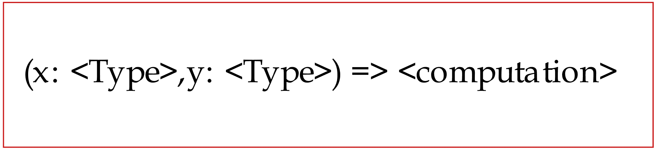
The Anonymous Function

An anonymous function is any that is not a named, reusable method – i.e, not introduced with the keyword def in Scala. It is also known as a function literal, and more universally, as a lambda expression. I’ll use anonymous function and lambda interchangeably. The arrow symbol => separates the bound parameters, if any, from the computation. Bound variable names are arbitrary.

Figure 1. A Scala anonymous function with two bound parameters

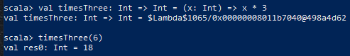
This basic example next shows a variable bound to an anonymous function and its invocation. Variable timesThree represents an unnamed function of type Int (integer) to Int – left of = – that is defined as taking an Int argument x and returning a transformed Int value.

Text Description automatically generated

Figure 2. One of several ways to define and use an anonymous function

Colons indicate variable types and return type.

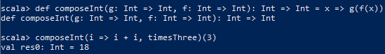
A higher-order function takes a function(s) as a parameter(s) and/or returns a function. Thus, an anonymous function, a variable such as timesThree, or a named method could all be arguments.

Text Description automatically generated

Figure 3. A well-known kind of higher-order function

Higher-order method composeInt takes two function parameters and does a common operation. Without providing the x value (3) argument, the return is a lambda as was echoed to screen (Int => Int).

NOTE: These examples were done in PowerShell. To try this on Windows, you must set up the Java JDK and Scala. Some websites, though, let you enter and run Scala code in a browser – just learn the println() command.

Two important higher-order functions are next.
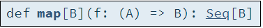
Map functions

A polymorphic function is one parameterized by type(s), allowing methods to be written generically, independent of instantiating type. A type can be the return type or type held by the returned containing object, and/or type of a parameter(s).

Known by varying names in possibly all FP languages are Scala’s polymorphic functions map() and flatMap().

Figure 4. A higher-order polymorphic function for sequence collections

Type parameters in Scala are in square brackets. The Seq trait is a supertype for sequence collections such as list and vector.

Part I showed that declarative T-SQL code could be translated into a loop implementation by the query optimizer. In a similar vein, map() abstracts looping over all collection elements, applying the polymorphic function ‘f’ parameter to each element. This is the result:

The original collection is unchanged; a new collection of the same class – in this example, a Seq subclass – holding the transformed elements of type B is returned.

Type B may or not be the same as type A, held in the original collection.

The map() can be chained with other map() calls and other operations but is not suited to nest another map() to simulate a nested loops pattern. This requires a more powerful form of map function.

Figure 5. The flatMap function signature

The IterableOnce trait is a more general base for all traversable data structures, as it covers the sequences in examples here as well as Sets and Maps and some non-collection types as well.

The background ends here. You will see maps and other higher-order functions in the solutions.

Solution space: IceCream trait

Having the download file IceCream_client.scala open aids the discussion. The commented code file also has many features and tests I won’t cover in this article. Make sure you have the latest version of the file, as it has changed since the release of the first article.

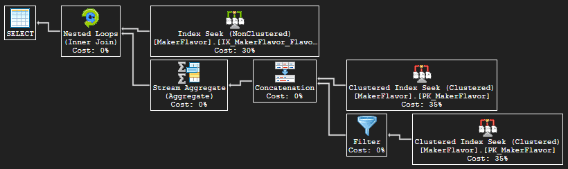
Recall the T-SQL query plan from Part I:

A screenshot of a computer Description automatically generated with medium confidence

Figure 6. Query plan from Section ‘Query Rewrite II’

The subtopic covers translating the plan into methods and index simulators in Scala.

Mirroring the T-SQL Query Plan

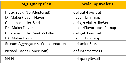
The following table shows the mapping from query plan items – the T-SQL blueprint above – to Scala pure functions and index simulators. Both will be covered in detail in subsequent topics.

Table Description automatically generated

Figure 7. Query plan to Scala mapping

Notice that there isn’t a precise correspondence from T-SQL to Scala objects. In rows two and three, the clustered index seeks, which use the primary key, reflect to different Scala methods and index simulators. In rows one and three, two different index seek types and index usage map to the same Scala method and index simulator.

Text Description automatically generated

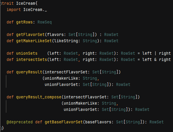
Figure 8. Trait as client interface

The IceCream trait in the figure above serves as the Scala client interface of available methods.. Two are defined in the trait, and the rest are abstract. Additional methods, some of which to be discussed, are documented in the download Scala file.

Since most relational tables have primary keys, they are sets, whether well-normalized (redundancy-free) or not. The query plan operators in the rewrite produce and work with denormalized sets of rows. In parallel, almost all trait functions return RowSets and have Set or RowSet parameters. This is by design. RowSet – meant to be intuitively named – is defined anon.

Client software now needs a way to create the object that implements the IceCream contract.

Solution space: IceCream companion object

Some data types in the trait are user-defined aliases from the companion object.

Graphical user interface, text Description automatically generated

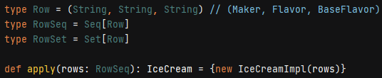
Figure 9. Type aliases and factory method

A Row is a three-tuple of strings representing (Maker, Flavor, Base Flavor). Types RowSeq and RowSet, then, are sequence and set parameterized data types holding the tuples. Tuple components are referenced with _x position notation, where x is 1,2,3…

The apply() function in companion objects has special meaning: it is a factory method clients use for creating the implementing object. In the IceCream project, the companion creates its own private class, passing it the RowSeq data, and returns the trait interface. This hidden implementation/separation of concerns style is a common design paradigm.

The object’s private class IceCreamImpl extends – roughly, inherits – the trait and encapsulates the resources for doing all data transformations.

Solution Space: IceCream Implementation

I’ll now broaden the meaning of ‘blueprint’ to include the query plan (Figure 6), its mapping to Scala equivalents (Figure 7), and the IceCream trait interface (Figure 8). Hidden class IceCreamImpl now has its pattern.

Figure 10. Implementation class’ initial data and trait extension

The rows in the parameter list is the OS file data, and keyword extends is analogous to OOP inheritance but follows different rules (not covered).

The two subtopics cover building the index simulators and realizing the interface. All code is within class IceCreamImpl.

Class construction: Index creation

T-SQL indexes (roughly) translate to key-value (k-v) pairs, which equate to the Map data structure. I’ve set up keys and values using a trait and case classes. A trait can be used solely for grouping related items, and a case class, for purposes here, is a class created without keyword ‘new’ and whose constructor parameters are default public.

A screenshot of a computer Description automatically generated with medium confidence

Figure 11. Structures used by index simulators

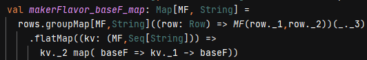
From the blueprint, primary key index PK_MakerFlavor has a compound key (Maker, Flavor) to which MF corresponds. In figure next, the Map is built from the initial data using several map functions:

Text Description automatically generated

Figure 12. The primary key equivalent

In the first code line (rows.groupMap…), in its first argument list (currying – not covered), the Map key is set to the composite key equivalent MF for every element in list rows. Put more explicitly: function groupMap iterates over every three-tuple (Maker, Flavor, Base Flavor) in the rows sequence of initial data, binding local variable row to each tuple at each pass. The entire argument – ((row: Row) => …) – is a lambda.

The second argument list sets the k-v value to the Base Flavor (shorthand tuple access _._3, also a lambda). The result is a Seq[String], where String is base flavor. This, though, is misleading. Per the business rules (Part I), a single value, not an ordered sequence of values, is correct and clearer. This is done in the next two lines.

On the newly generated Map, its flatMap() – essentially, the outer loop – iterates over every k-v pair. The nested map() – inner loop – translates and returns each one-row sequence (kv._2) of base flavors into the k-v value. A k-v pair in Map is represented as (k -> v).

If you’ve never worked with functional programming, I hope you are reading for the gist of it and appreciate its compactness and elegance (among other benefits).

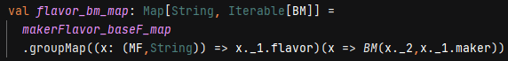
The IX_MakerFlavor_Flavor covering index simulator can be built from this primary key simulator:

Figure 13. The covering index equivalent

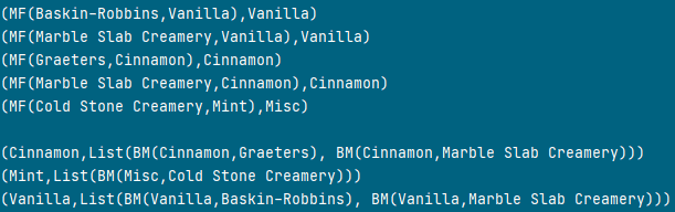
This time, again by the business rules, a sequence (list) of case class BM is correct, as sample output from both Map structures shows:

Graphical user interface, text Description automatically generated

Figure 14. Sample equivalent rows from primary key and covering index simulators

The covering index simulator flavor_bm_map restructures the data in the primary key simulator makerFlavor_baseF_map exactly as it happened in the database.

Serving the interface

For brevity, I won’t cover the entire trait interface – just enough to explore using the indexes and deriving solutions. Refer to T-SQL to Scala mapping Figure 7.

Text Description automatically generated

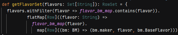
Figure 15. Simulating index seeks

Method getFlavorSet is invoked to emulate two different T-SQL query plan operators using index seeks over the IX_MakerFlavor_Flavor and PK_MakerFlavor indexes (rows 1 and 3). The former restricts on Mint, Coffee, Vanilla and the latter, Vanilla solely, as given in the flavors parameter.

Method withFilter is a non-strict filter, meaning – in usage here – that it doesn’t produce an intermediate set that must be garbage collected but rather restricts the flatMap domain during its traversal of elements. Its lambda argument simply eliminates any flavor not recognized as a key in flavor_bm_map rather than throwing or handling an exception.

The flatMap iterates over every recognized flavor. The flavor_bm_map(flavor) operation returns the list of BM (base flavor, maker) case classes – the value in the k-v – and the map function takes each to form an individual Row.

Text Description automatically generated

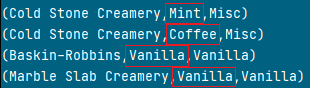
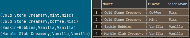
Figure 16. Query result over three flavors

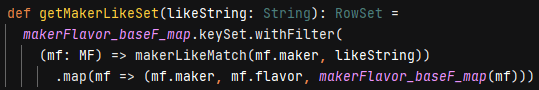
Method getMakerLikeSet corresponds to the upper Clustered Index Seek branch in the lower input to Nested Loops (row 2). The seek is done on the primary key index but is inefficient as its Predicate must tease apart the maker name. The method equivalent is worse.

Text Description automatically generated

Figure 17. The method finds all ‘Creamery’ makers (suboptimal)

The like argument trivially is ‘Creamery’. For every k-v key in the primary index simulator, the algorithm filters out all makers who aren’t ‘Creamery’ using a non-interface named method (not shown) rather than a lambda. (Without elaboration, a more optimal version is possible but involved.)

Deprecated function getBaseFlavorSet uses a third covering index simulator having base flavor as key. The first article proved why this index is not desired; here, as in the T-SQL, usage produces four rows to be culled later instead of the desired two. This was also proved in the Scala test run.

All needed methods and resources are now in place for IceCreamImpl to solve the series problem. Here is the first of two solutions:

Text Description automatically generated

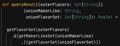
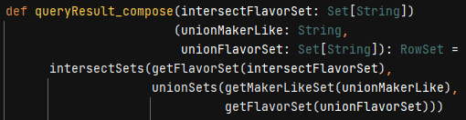
Figure 18. Equivalent to T-SQL query rewrite II (final form)

The first parameter outerFlavors contains the three flavors as discussed; the second, Creamery; and the third, Vanilla. The first invocation of getFlavorSet mimics the query plan outer input to Nested Loops. This set of three-tuple rows intersects (‘&’) with the rows simulating the inner input, thereby paralleling the Nested Loops’ Inner Join logical operation. The call to getMakerLikeSet retrieves the Creamery rows and does a union (‘|’) with the second invocation of the getFlavorSet. The union mirrors the Stream Aggregate ← Concatenation operators.

The second, equivalent solution, is more function composition style.

Text Description automatically generated

Figure 19. Solution in function composition

The blueprint has been realized in software. All that is left is to verify the result:

Table Description automatically generated with medium confidence

Figure 20. Software and T-SQL yield the same result set

The Client

Programming side effects include I/O, and these are limited exclusively to the client, which consumes the IceCream trait and companion object. The client reads the data from the OS file, packages it for consumption by the factory method in the companion, and invokes the pure functions in the trait, printing results to screen. For brevity, here is a snippet from the call to apply():

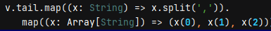
Figure 21. Transforming the OS file data for IceCream factory method apply()

Variable v holds the data from the .csv file as a sequence of strings, and the tail function skips past the (Maker, Flavor, BaseFlavor) header. The first map() transforms each line in the sequence (Seq[String]) to an array size three of strings (Array[String]). A second map() chains to the first to turn each array into a three-tuple.

In Conclusion

This second and last article in the series gave a condensed background in functional programming and Scala. This included higher-order, pure, and map functions and lambda arguments. All data transformations were done using these constructs, plus a non-strict filter method. In good functional programming style, all coding was declarative: no low-level control flow statements were written.

The notion of blueprint was widened, first by a translation grid that mapped T-SQL query plan operators and indexes to pure functions and Map types as index simulators. This led to the development of the IceCream trait client interface.

The trait was paired with a companion object whose major purpose was to expose a factory method (apply()) for creating the implementation object from a hidden (private) class and returning the IceCream interface to the client. The client’s responsibility was to supply the factory method with the OS file data. (Or data from any source.)

Last Word

In sum, the series presented my own methodology for solving a class of problems. I doubt you would disagree with adding SQL Server to the development environment as a means of verifying computations.

As for doing a deeper relational analysis to devise a query plan that can serve as model for software design, consider that data, regardless of source, can always be modeled relationally. By tinkering with database design, indexing, query patterns and plans, you might uncover insights you may not have discovered otherwise.

The post A data transformation problem in SQL and Scala: Dovetailing declarative solutions Part II appeared first on Simple Talk.


from Simple Talk https://ift.tt/3fijMoW
via

Thursday, March 25, 2021

What to monitor for SQL Server security

SQL Server databases are under greater threat than ever. Cyberattacks are on the rise, and they’re becoming more sophisticated with each new generation. And these aren’t the only risks. Organizations must also guard against insider threats, whether carried out by disgruntled employees or those engaged in more nefarious activities. At the same time, organizations must contend with a growing number of compliance regulations, such as the General Data Protection Regulation (GDPR), Health Insurance Portability and Accountability Act (HIPAA), and the California Consumer Privacy Act (CCPA).

To meet today’s security and compliance challenges, SQL Server DBAs and other security professionals need to implement comprehensive protection plans that safeguard their data, databases, and the environments in which they operate. One of the most important steps they can take is to monitor their SQL Server instances, auditing events that can indicate a threat against sensitive data.

If you’re one of those people charged with monitoring a SQL Server environment, you should capture all metrics that can help reveal possible risks, whether failed logins, altered permissions, schema changes, or anything else. You might be tempted to audit every available metric just to play it safe, but such an approach comes with significant overhead. You need to focus on those events that are the most relevant to your circumstances, taking into account applicable regulations and the type of data being stored.

Although there is no one-size-fits-all solution when it comes to a monitoring strategy, there are specific areas of concern that you should consider when determining the best approach to auditing your SQL Server environments. In general, you should monitor SQL Server access controls, SQL Server objects and configurations, and data access behavior. Even though these are broad fields, they provide a good starting point for defining a monitoring plan based on your specific needs.

SQL Server access controls

SQL Server includes several internal mechanisms for authenticating users to a SQL Server instance and controlling their access to data, using a combination of security principals, securables, and permissions. Principals are individuals, groups, or processes that are granted access to a SQL Server instance at the server level or database level. Securables are the objects that make up the SQL Server environments, such as databases, schemas, tables, functions, logins, or roles. Permissions define the level of access that is granted or denied to principals on specific securables.

Monitoring SQL Server access should be an important part of any auditing strategy because it provides direct insight into who can view or modify sensitive data or whether there are any suspicious efforts to access the data. For example, monitoring failed login attempts can help you detect brute force attacks or other malicious behavior. But that is only one metric. You should also consider tracking the following access-related events:

  • Security principals being added or dropped, whether at the server level or database level
  • Members being added to or deleted from server or database roles
  • Permissions being granted or denied to server, database, and schema securables

Changes in any of these three areas can indicate attempts at fraud or data threats. Once the changes are made, your databases might be vulnerable to data exposure, compliance violations, or disruptions in services. For example, a cybercriminal might gain access to a SQL Server instance and then modify the permissions in order to bulk-copy data out of a database or to run a malicious stored procedure. Access control changes can also indicate that someone inside your organization is being careless or is up to no good.

By monitoring access controls, you can identify a wide range of potential risks. For example, someone might have enabled the sa account, modified permissions on the SQL Server service account, or added members to the db_owner or sysadmin roles. Whether these actions are carried out intentionally or through sloppiness, they can all put a database at risk.

The decision on which access controls to monitor might be driven in good part by prevailing regulations, which often have strict guidelines on what information you need to track, but overall security concerns should also be part of your thinking, even if you’re not subject to a specific set of rules.

SQL Server objects and configurations

In addition to tracking access controls, you should also monitor changes to SQL Server objects at the server, database, and schema levels. In this way, you can audit changes that can put sensitive data at risk in ways not apparent through monitoring access controls. For example, a compromised login might go undetected, but it’s not until you see schema changes such as a dropped table or added function that you realize something is wrong.

As with other aspects of SQL Server monitoring, the exact approach you take to auditing SQL Server objects will depend on applicable regulations and the type of data in your database. However, there are certainly objects that stand out above the rest.

For example, you might find it useful to track activity related to the database objects themselves, such as when a database is created, altered, or dropped or whether it’s been stopped, started, attached, detached, gone offline, or brought back online. You might even want to know if a database’s size has changed and, if so, how much. The goal is to always be on top of changes to the databases so that you know which ones have changed, how they were changed, who changed them, and when the changes occurred.

That said, you need to monitor more than just the database objects to determine whether there’s been any tampering. For a clearer picture, you should also track changes at a more granular level, especially when it comes to objects that store sensitive data. For example, you might want to audit changes to a database’s schema objects so you can see which ones have been recently created, altered, or dropped or have been assigned a new owner. This type of auditing can also help you detect database drift, which comes with its own security concerns.

In addition to monitoring SQL Server objects, it can also be useful to audit changes to configuration settings. For example, a cybercriminal might have gained high-level access to a SQL Server instance and enabled CLR in order to launch a malicious assembly. If you were alerted to that change, you might have enough time to prevent that assembly from running and doing any damage.

Even if configuration changes aren’t the result of an attack, they’re still worth knowing about. For instance, a DBA might have enabled the xp_cmdshell extended stored procedures on a production server to pull down data and then forgot to disable it. Although it wasn’t done with malicious intent, it could still have serious consequences.

Monitoring SQL Server for configuration changes at the server and database levels can help detect threats that might otherwise be missed, but this approach is only effective if you actually catch the change. It doesn’t tell you what the configuration settings are supposed to be or whether any current settings are wrong. For this reason, you might also need to establish a base of agreed-upon settings that you can refer to for the absolute truth—the type of information often stored in a database configuration management archive (DCMA).

Data access behavior

Monitoring changes to SQL Server objects and configurations is extremely important, as is tracking access controls, but they might still not be enough to catch all threats or be in compliance with current regulations. You might also need to track access to the data itself, especially if regulations require it. For example, you might have to audit all SELECT access to each table that contains sensitive data. In this way, you can establish an audit trail of who accessed what data and when that access occurred, details you must often provide during a compliance audit.

You should also consider monitoring other types of events related to data access. One example would be to track whether anyone has used the BCP utility to bulk copy data out of a table. Another example would be to determine whether someone has issued a BACKUP statement, which could indicate the presence of an illegal database copy. Any metrics that can point you to potential data compromise are worth serious consideration.

In some cases, you might need to track data modifications instead of or in addition to data access. Regulations such as HIPAA and the Sarbanes-Oxley Act (SOX) require that you protect sensitive data against wrongful deletions or modifications, whether accidental or intentional. If either of these regulations applies to you, you’ll need to track all data modifications and deletions in order to demonstrate compliance. To do this effectively, however, you should audit database-level object changes, as well as INSERT, UPDATE, and DELETE activity. You should also be able to determine how the data has changed so you can compare before and after values.

In addition to monitoring data access and modifications, it can also be important to track SQL errors, which can point to SQL injection attacks or other threats. Would-be hackers often issue multiple SQL statements against a database to deliberately trigger SQL errors in an effort to navigate the schema. For example, a hacker attempting to carry out injection attacks might try to access invalid objects or use incorrect SQL syntax to glean schema information from the error messages.

Other monitoring considerations

You can go a long way in protecting your SQL Server environment by monitoring access controls, objects and configurations, and data access behavior. But a complete monitoring solution must also take into account factors such as the following:

  • Applications that access data in SQL Server databases should be monitored for unusual usage patterns or business processes or for any other suspicious activity.
  • The Windows Server computer that hosts SQL Server should be monitored for suspicious activity. Cybercriminals might be able to gain access through server logins and then change server settings or compromise SQL Server database files.
  • In addition to monitoring the SQL Server environment, you should also audit the monitoring tools and processes themselves. You must be able to ensure that no one has tampered with the auditing process and that your monitoring solution is as secure as the SQL Server data.
  • Effective monitoring often includes the ability to detect unusual usage patterns in how the SQL Server instance is managed and how data is accessed and modified. For this, you might need to create baselines that represent acceptable patterns that can then be compared to the audited events.

Another important factor in monitoring SQL Server is to ensure you have the right tools in place to help you audit selected metrics as efficiently as possible. You should also be able to track trends and to be alerted to behavior that represents an immediate threat. SQL Server Audit provides a good tool for auditing events, but it comes with limitations. One of the biggest is that it’s built into SQL Server. An attacker that gains access to the platform could disable the auditing features and other security protections. With a third-party tool such as Redgate’s SQL Monitor, you get a system separate from SQL Server, along with advanced features that help simplify the monitoring process.

Implementing a SQL Server monitoring strategy is no small feat. It requires careful planning and ongoing diligence to ensure that you’re protecting your sensitive data and complying with applicable regulations. Your monitoring solution should meet your specific requirements based on your current circumstances, with the understanding that those circumstances can change. SQL Server monitoring should also be implemented in concert with other security measures to help guarantee that your systems and data are protected at all times. In today’s climate, data security must be a top priority, and monitoring SQL Server is one of the most important steps you take, but you have to do it right to protect your data to its fullest.

If you liked this article, you might also like SQL Server authentication methods, logins, and database users.

The post What to monitor for SQL Server security appeared first on Simple Talk.


from Simple Talk https://ift.tt/3d7mjPO
via

Wednesday, March 24, 2021

To soon?

I’ve noticed that some television shows have been incorporating the Covid-19 pandemic into their recent episodes. (There are some spoilers here, so read with caution!) A medical series, “The Good Doctor,” featured it in two episodes and then, magically, the pandemic was over. The popular series “This is Us” is trying to set a good example by making sure that the characters wear masks when meeting up with people outside of their households — until they actually walk up to each other to talk. Then the masks come off. I’ve heard that acting on TV is about facial expressions, so it makes sense that the producers don’t want faces hidden. The pandemic is sort of the background but doesn’t overwhelm the storyline.

Another series, “A Million Little Things,” seems painfully accurate. A restaurant owner sees her business crumble as staff call off sick and customers stay home. Another character is about to shoot his first movie and production stops, ending, or at least postponing, his life’s dream. Borders shut down keeping some characters from traveling home. The characters are confused about what is going on and how long it will last, just like we were a year ago. This is all too real.

Watching the events that have happened over the past year be incorporated into entertainment is inevitable, but maybe it is too soon. People continue to suffer, and lives have been turned upside down. While there is a bit of light at the end of the tunnel as vaccines become more available, that tunnel is long. We don’t know yet how this turns out, so it’s painful to watch when all you want is to be entertained.

On the other hand, dystopian fiction featuring plagues of some sort has been around for decades, maybe longer. It’s fun to read books or watch movies where the world has gone mad while safely sitting in a comfy chair. It feels quite different when events around you resemble the story.

Commentary Competition

Enjoyed the topic? Have a relevant anecdote? Disagree with the author? Leave your two cents on this post in the comments below, and our favourite response will win a $50 Amazon gift card. The competition closes two weeks from the date of publication, and the winner will be announced in the next Simple Talk newsletter.

The post To soon? appeared first on Simple Talk.


from Simple Talk https://ift.tt/3tUdmQz
via

Tuesday, March 23, 2021

Mastering TempDB: Managing TempDB growth

The series so far:

  1. Mastering TempDB: The basics
  2. Mastering TempDB: Managing TempDB growth

As you learned in part one of this Mastering TempDB series, TempDB is a global resource used for many operations within SQL Server. You create and allocate temporary user objects such as temporary tables and table variables, rebuild indexes with SORT_IN_TEMPDB=ON, use it for version stores (RCSI), internal objects (worktables, spools, group by, order by) and even DBCC CHECKDB just to name a few. All these operations require space to be allocated in the TempDB database. At times, these operations can result in TempDB growing rapidly, which, in turn, can fill up the file system and cause failures. In this article, you will learn how to fix an overgrown TempDB file that has resulted in it running out of space.

Uncontrolled TempDB growth

There are many reasons for uncontrolled TempDB growth events. Much like your operating system has a page file to handle memory overflows, SQL Server uses TempDB like a page file. The most common occurrence of this is when a query “spills” to TempDB. When you execute a query, the database engine allocates memory to perform join and sort operations. The amount of memory allocated is based on the statistics associated with the columns and indexes. If the estimate is incorrect and the engine does not allocate enough memory, those joins and sorts will spill to disk—which consumes a lot of TempDB resources. Spilling is only one use of TempDB; some of the other ways SQL Server uses this database include storing large temporary tables. Temp tables can lead to uncontrolled growth if they are being populated by a query that needs to be tuned. You could have an Availability Group replica, which runs in snapshot isolation mode, go down, which causes the version store to fill up. You can have a normal workload cause TempDB to have an auto-growth that causes you to run out of drive space. There are countless explanations as to why TempDB can grow. The key administrative task is not only trying to get the drive space back and the system running, but also identifying the cause of the growth event to prevent recurrence.

As a reminder from the first article, you can easily peek inside your TempDB database to see what has caused the file to fill up. These great queries below provided in TempDB msdocs is a good place to start. Once you locate the culprit, you can tune accordingly to prevent the issue from reoccurring.

-- Determining the amount of free space in tempdb
SELECT SUM(unallocated_extent_page_count) AS [free pages],
  (SUM(unallocated_extent_page_count)*1.0/128) AS [free space in MB]
FROM sys.dm_db_file_space_usage;
-- Determining the amount of space used by the version store
SELECT SUM(version_store_reserved_page_count) 
   AS [version store pages used],
  (SUM(version_store_reserved_page_count)*1.0/128) 
   AS [version store space in MB]
FROM sys.dm_db_file_space_usage;
-- Determining the amount of space used by internal objects
SELECT SUM(internal_object_reserved_page_count) 
   AS [internal object pages used],
  (SUM(internal_object_reserved_page_count)*1.0/128) 
   AS [internal object space in MB]
FROM sys.dm_db_file_space_usage;
-- Determining the amount of space used by user objects
SELECT SUM(user_object_reserved_page_count) 
   AS [user object pages used],
  (SUM(user_object_reserved_page_count)*1.0/128) 
   AS [user object space in MB]
FROM sys.dm_db_file_space_usage;

If you use SQL Monitor, you can also view what’s going on in the new tempdb section.

SQL Monitor shows tempdb growth

The following script is my go-to that I have used for years to reactively and proactively understand what’s going on inside TempDB. It was adapted from Microsoft by Kendra Little (B|T) back in 2009 and is still an excellent tool for analyzing TempDB workloads. This script’s query results allow you to clearly identify what space is allocated by a transaction and even capture the query text and its execution plan associated with it.

SELECT t1.session_id,
       t1.request_id,
       task_alloc_GB = CAST((t1.task_alloc_pages * 8. / 1024. / 1024.) 
         AS NUMERIC(10, 1)),
       task_dealloc_GB = CAST((t1.task_dealloc_pages * 
          8. / 1024. / 1024.) 
         AS NUMERIC(10, 1)),
       host = CASE
                  WHEN t1.session_id <= 50 THEN
                      'SYS'
                  ELSE
                      s1.host_name
              END,
       s1.login_name,
       s1.status,
       s1.last_request_start_time,
       s1.last_request_end_time,
       s1.row_count,
       s1.transaction_isolation_level,
       query_text = COALESCE(
                    (
                  SELECT SUBSTRING(
                    text,
                    t2.statement_start_offset / 2 + 1,
                    (CASE
                     WHEN statement_end_offset = -1 THEN
                        LEN(CONVERT(NVARCHAR(MAX), text)) * 2
                     ELSE
                        statement_end_offset
                     END - t2.statement_start_offset
                                            ) / 2
                                        )
                        FROM sys.dm_exec_sql_text(t2.sql_handle)
                    ),
                    'Not currently executing'
                            ),
       query_plan =
       (
           SELECT query_plan FROM sys.dm_exec_query_plan(t2.plan_handle)
       )
FROM
(
    SELECT session_id,
           request_id,
           task_alloc_pages = SUM(internal_objects_alloc_page_count 
               + user_objects_alloc_page_count),
           task_dealloc_pages = SUM(internal_objects_dealloc_page_count 
                + user_objects_dealloc_page_count)
    FROM sys.dm_db_task_space_usage
    GROUP BY session_id,
             request_id
) AS t1
    LEFT JOIN sys.dm_exec_requests AS t2
        ON t1.session_id = t2.session_id
           AND t1.request_id = t2.request_id
    LEFT JOIN sys.dm_exec_sessions AS s1
        ON t1.session_id = s1.session_id
-- ignore system unless you suspect there's a problem there
WHERE t1.session_id > 50 
 -- ignore this request itself 
AND t1.session_id <> @@SPID
ORDER BY t1.task_alloc_pages DESC; 
GO

Here are a couple screenshots of the output.

This one shows active row counts, but there is not a ton of space allocated.

This one shows only one row as a row_count, but look at the task_alloc_GB column. Even though it is only one row, this transaction is taking 1.6GB of space.

Once you identify the culprit, you can move on to resizing. I highly advise you to pause and look at the causal factors before trying to resize, since it is possible to lose all purview to that information. Many of these commands are destructive and will cause you to lose metadata associated with your TempDB growth–this means it is important to capture.

Resizing TempDB

Occasionally, we must resize or realign our TempDB log file (.ldf) or data files (.mdf or .ndf) due to a growth event that forces the file size out of whack. To resize TempDB we have three options, restart the SQL Server service, add additional files, or shrink the current file. We most likely have all been faced with runaway log files, and, in an emergency situation, restarting the SQL Services may not be an option, but we still need to get our log file size smaller before we run out of disk space, for example.

Restart SQL Server Services– since TempDB is non-durable, it is recreated upon service restart at the file size and count that are defined in the sys.master_files catalog view.

Add File– You can quickly get out of trouble by adding another TempDB.mdf file to another drive that has space. This will buy you some time but should be removed once the issue is resolved and your services can be restarted. I only use this one in a true emergency. If you add a file you should plan a restart of your SQL Services because it will now be the most free space file, and your workload will funnel here. So be sure to balance them by restarting to ensure the most efficient round robin use.

Shrink Files– This removes unused space and resizes the file. I’ll explain this process below.

The process of shrinking a datafile can get tricky, so I created this flow chart to help you out if you ever get into this situation. It’s very important to note that many of these commands will clear your cache and will greatly impact your server performance as it warms cache back up. In addition, you should not shrink your database data or log file unless absolutely necessary, but doing so can result in a corrupt tempdb.

Let’s walk through it, and I’ll explain some things as we go along.

tempdb growth shrinking diagram

First thing you must do is issue a Checkpoint. A checkpoint marks the log as a “good up to here” point of reference. It lets the SQL Server Database Engine know it can start applying changes contained in the log during recovery after this point if an unexpected shutdown or crash occurs. Anything prior to the checkpoint is what I like to call “Hardened”. This means all the dirty pages in memory have been written to disk, specifically to the .mdf and .ndf files. So, it is important to make that mark in the log before you proceed. While TempDB is recreated and not recovered during a restart, however, this is still a requirement of this process.

USE TEMPDB;  
GO  
CHECKPOINT;

Next, we try to shrink the log and data files by issuing DBCC SHRINKFILE commands. This is the step that frees the unallocated space from the database file if there is any unallocated space available. You will note the Shrink? decision block in the diagram after this step. It is possible that there is no unallocated space, and you will need to move further along the path to free some up and try again.

USE TEMPDB;  
GO 
DBCC SHRINKFILE (templog, 1024);   --Shrinks it to 1GB
DBCC SHIRNKFILE (tempdev, 1024);

If the database shrinks, great, congratulations! However, some of us might still have work to do. Next up is to try to free up some of that allocated space by running DBCC DROPCLEANBUFFERS and DBCC FREEPROCCACHE.

DBCC DROPCLEANBUFFERS – Clears the clean buffers from the buffer pool and columnstore object pool. This command will flush cached indexes and data pages.

DBCC DROPCLEANBUFFERS WITH NO_INFOMSGS;

DBCC FREEPROCCACHE – Clears the procedure cache. You are probably familiar with as a performance tuning tool in development. It will clean out all your execution plans from cache, which may free up some space in TempDB. This will create a performance issue as your execution plans now have to make it back into cache on their next execution and not benefit from plan reuse.  It’s not really clear why this works, so I asked TempDB expert Pam Lahoud (B|T) for clarification as to why this has anything to do with TempDB. Both of us are diving into this to understand exactly why this works. I believe it to be related to TempDB using cached objects and memory objects associated with stored procedures which can have latches and locks on them that need to be released by running this. Check back for further clarification, as I’ll be updating this as I find out more.

DBCC FREEPROCCACHE WITH NO_INFOMSGS;

Once these two commands have been run and you have attempted to free up some space, you can now try the DBCC SHRINKFILE command again. For most, this should make the shrink possible, and you will be good to go.  Unfortunately, a few more of us may have to take a couple more steps through to get to that point.

When I have no other choice to get my log file smaller I run the last two commands in the process. These should do the trick and get the log to shrink.

DBCC FREESESSIONCACHE– This command will flush any distributed query connection cache, meaning queries that are between two or more servers.

DBCC FREESESSIONCACHE WITH NO_INFOMSGS;

DBCC FREESYSTEMCACHE – This command will release all unused remaining cache entries from all cache stores, including temp table cache. This covers any temp table or table variables remaining in cache that need to be released.

DBCC FREESYSTEMCACHE ('ALL');

Manage TempDB growth

In my early days as a database administrator, I would have loved to have this diagram. Having some quick steps during stressful situations such as TempDB’s log file filling up on me would have been a huge help. Hopefully, someone will find this handy and be able to use it to take away a little of their stress.

Remember, it is important for you to become familiar with how your TempDB is used, tune those queries that are large consumers and know how to properly resize TempDB if it becomes full.


The post Mastering TempDB: Managing TempDB growth appeared first on Simple Talk.


from Simple Talk https://ift.tt/2Pf6pea
via