Monday, October 25, 2021

Routing Access to Azure Services

Azure is part of the Microsoft Global Network. Applications in the Azure environment can receive access from the entire world. This world-wide access creates a dilemma about the routing to the Azure services. We face two options: routing through Microsoft Global Network or through public internet.

Initially only the Storage Accounts had a direct configuration about this routing access. Nowadays, we can configure the routing access in any Public Ip using Standard SKU.


This means that any service linked to a Public IP object defined in azure can have its routing preferences configured. This affects most IaaS features, such as virtual machines. However, load balancers and application gateways are also affected and they may be the front-end for PaaS services. Traffic Manager and Azure Front Door are some feature that allow us to manipulate these routing preference in an indirect way.

What the Routing Options mean

The routing options are called Microsoft Routing and Internet Routing. It’s about the way the access will be routed from the user to the Azure service.

When the communication starts on the user machine, the communication is starting outside Microsoft Global Network and will cross some ISPs hardware until it gets to the MS Global Network. How many routers outside Microsoft environment will be routing the packages of this communication?

That’s the difference the routing preference makes:

  • Internet Routing will make the package get into the Microsoft Global Network from the closest possible point to the resource. In this way, the package will flow on the public internet most of the way until the destination.

  • Microsoft Network will make the package get into the Microsoft Global Network from the closest possible point to the user. In this way, the package will flow inside Microsoft Global Network most of the way until the destination.

The Implications

The security implications are obvious. The most the package flows inside Microsoft Global Network, safer the package is. However, since we are given these options there must be something else to this choice.

There is: The networking price. There is a difference price for network packages that cross Azure regions and continents. This price will make the cost of the cloud higher.

The main question that everyone asks is: How higher?

You can see details about the difference of traffic across regions and continents on this link: https://azure.microsoft.com/en-us/pricing/details/bandwidth/


A good way to summarize this link is by highlighting the difference of the traffic from South America to other regions when your service is located in South America. If you move 10 TB every month, it would cost you around us$ 1,200.00 if you are using internet routing but around us$ 1,800.00 if you are using Microsoft routing.

Mind these highlights about this example:

  •  South America is the most expensive region in relation to trafic and the one with the biggest difference between Internet and Microsoft routing
  • 10 TB is huge amount of data. Consider many ways your application may avoid such huge traffic, like using CDN and other cache features. Most solutions will not reach this amount of traffic.
  • The price drops after 10 TB/month

In my humble opinion, the price difference is insignificant to make someone choose internet routing instead of Microsoft routing.

Indirect routing Management

Besides services linked with public Ip and the Azure Storage, we can indirect manage this routing problem by using Azure Front Door or Azure Traffic Manager. These two load balancers are DNS based solutions distributed globally. Wherever the user is in the globe, it will reach the endpoints of these services from the closest Microsoft network endpoint possible. After that, the rules of these load balancers take place and decide what service in our company global virtual network will provide the end user service.

It’s a choice to use or not these load balancers and to distribute or not our services around the globe. If we choose not to, the user packages will need to reach the physical place of our application, whatever region we choose for it. Using these tools, on the other hand, we have the option to redirect the traffic to the application server we provisioned closest to the user.


References

https://docs.microsoft.com/en-us/azure/virtual-network/ip-services/routing-preference-overview

The post Routing Access to Azure Services appeared first on Simple Talk.


from Simple Talk https://ift.tt/3GiHpbL
via

Cache strategies in Redis

Redis is a cache database that stores documents in memory. The data store has a key-value pair lookup with O(1) time complexity. This makes the cache fast and convenient because it does not have to deal with complex execution plans to get data. The cache service can be trusted to find a cache entry with a value in almost no time.

When datasets in cache begin to grow, it can be surprising to realize that any latency is not a Redis issue. In this take, I will show you several strategies to cache Redis data structures then show what you can do to pick the best approach.

The sample code can be found on GitHub, and it is written in C# via .NET 5. If you already have LINQPad up and running, feel free to copy-paste code and follow along.

There are a few dependencies. You will need a Redis Windows service when running this on Windows 10. I recommend grabbing binaries from GitHub and setting up the server on your local machine. You can quickly have a server running by executing redis-server.exe. I will be hammering the service with lots of cache data, so I recommend setting the maxmemory to something high like 50MB. A full Redis installation on Windows should take no more than 6MB because it is lightweight. For the C# code, you will need two NuGet packages: protobuf-net and StackExchange.Redis, as well as ProtoBuf and StackExchange.Redis using statements.

These are the caching strategies:

  • Binary
  • XML
  • JSON
  • ProtoBuf

.NET serializers allow you to work with document data cached in Redis. On the server-side, all Redis does is store and retrieve arbitrary blob data. The key-value pair can be as big as it needs to be, assuming it can fit in-memory. It is up to the C# code to decide what to do with this data stream and determine which serialization strategy to use. Any performance issues you may stumble upon have to do with how long this serialization process takes. It is the client code, not the cache server, that does the actual work.

Connecting to Redis

First, put this skeleton app in place. It will need to instantiate a Redis connection, grab a Stopwatch, and declare DTOs.

const int N = 50000;
var redis = ConnectionMultiplexer.Connect("localhost");
var db = redis.GetDatabase();
var stopWatch = new Stopwatch();
// The rest of the code goes here
[Serializable]
record BinaryDto(
  string propertyA,
  string propertyB,
  string propertyC,
  Guid id);
public record XmlDto(
  [property: XmlElementAttribute()]
  string propertyA,
  [property: XmlElementAttribute()]
  string propertyB,
  [property: XmlElementAttribute()]
  string propertyC,
  [property: XmlAttribute()]
  Guid id)
{
  XmlDto() : this(
    string.Empty,
    string.Empty,
    string.Empty,
    Guid.Empty) {}
};
record JsonDto(
  string propertyA,
  string propertyB,
  string propertyC,
  Guid id);
  
[ProtoContract(SkipConstructor = true)]
record ProtoDto(
  [property: ProtoMember(1)]
  string propertyA,
  [property: ProtoMember(2)]
  string propertyB,
  [property: ProtoMember(3)]
  string propertyC,
  [property: ProtoMember(4)]
  Guid id);

The key code to look at here is the DTO records. I have declared a separate DTO per strategy. To serialize data in binary, it needs the Serializable attribute. For XML, it needs a default public constructor and property attributes. This is how the XML document takes shape; for example, the id property will go on the parent node as an attribute, and the rest of the XML properties will be declared as children. The JSON data object does not have any ceremonial code. ProtoBuf needs positional ordinals, which are set via an integer. It does not matter what the order is as long as the proto members are unique. Setting the proto contract to skip the constructor makes this serializer work with records.

There are no real performance benefits to using records here other than to keep the C# code nice and terse. These DTOs will be instantiated as lists and will live in the heap anyway.

I declared a constant N to set the size of the dataset that is going into Redis. This is set to fifty thousand records. Depending on the size of your specific cache, I recommend changing this value to fit your needs. ProtoBuf, for example, is not the best strategy for small payloads. This is because there are no one size fits all solutions.

One caveat for XML, the shape of element attributes will dictate the size of the payload. XML tends to be verbose, and setting more properties as attributes on the parent node will reduce its overall size. I opted to include both techniques mostly to show there are ways to change the payload without changing strategies altogether. Feel free to play around with the XML serializer to double-check how this impacts performance.

Binary serializer

To serialize data in binary, instantiate a list of records and set/get the cache entry in Redis.

var binaryDtoList = Enumerable.Range(1, N)
  .Select(i => new BinaryDto(
    "PropertyA" + i,
    "PropertyB" + i,
    "PropertyC" + i,
    Guid.NewGuid()))
   .ToList();
stopWatch.Start();
using (var binarySetStream = new MemoryStream())
{
  var binarySerializer = new BinaryFormatter();
  binarySerializer.Serialize(binarySetStream, binaryDtoList);
  db.StringSet(
    "binary-cache-key",
    binarySetStream.ToArray(),
    TimeSpan.FromMinutes(5));
}
stopWatch.Stop();
Console.WriteLine($"Binary write = {stopWatch.ElapsedMilliseconds} ms");
stopWatch.Restart();
var binaryCacheEntry = db.StringGet("binary-cache-key");
using (var binaryGetStream = new MemoryStream(binaryCacheEntry))
{
  var binaryDeserializer = new BinaryFormatter();
  binaryDeserializer.Deserialize(binaryGetStream);
}
stopWatch.Stop();
Console.WriteLine($"Binary read = {stopWatch.ElapsedMilliseconds} ms");
Console.WriteLine();

The StringSet sets data in Redis, and StringGet gets the data. These methods are a bit of a misnomer because the cache entry stored in Redis isn’t in string format but binary. It is not the same binary representation used by the serializer but one internal to Redis when it gets or sets its data. When setting a cache entry, be sure to specify a key. Retrieving the cache entry is as easy as getting the data stream via the same cache key. The TimeSpan argument allows the cache entry to expire after a certain time limit.

With your Redis server running , first, run the project. Then, run the redis-cli.exe executable in a command line and type in GET "binary-cache-key".

This is what you might see:

Text, letter Description automatically generated

The CLI tool shows a string representation of the underlying blob data. An important takeaway is that I can see bits and pieces of the underlying record like “PropertyA49999”. This took 3.74 seconds to deserialize this dataset which gives you a good indication of the performance. The C# client is much faster than this, but the sheer size of this payload can impact overall performance.

If you are on .NET 5, you may see a helpful build warning when working with the binary serializer. This warning points out the fact that the BinaryFormatter is obsolete. For security reasons, it is recommended to move away from this regardless of performance. I put this serializer here mainly to show how it stacks up against other alternatives.

XML serializer

Time to put the XML serializer to the test.

var xmlDtoList = Enumerable.Range(1, N)
  .Select(i => new XmlDto(
    "PropertyA" + i,
    "PropertyB" + i,
    "PropertyC" + i,
    Guid.NewGuid()))
   .ToList();
stopWatch.Start();
using (var xmlSetStream = new MemoryStream())
{
  var xmlSerializer = new XmlSerializer(xmlDtoList.GetType());
  xmlSerializer.Serialize(xmlSetStream, xmlDtoList);
  db.StringSet(
    "xml-cache-key",
    xmlSetStream.ToArray(),
    TimeSpan.FromMinutes(5));
}
stopWatch.Stop();
Console.WriteLine($"Xml write = {stopWatch.ElapsedMilliseconds} ms");
stopWatch.Restart();
var xmlCacheEntry = db.StringGet("xml-cache-key");
using (var xmlGetStream = new MemoryStream(xmlCacheEntry))
{
  var xmlDeserializer = new XmlSerializer(xmlDtoList.GetType());
  xmlDeserializer.Deserialize(xmlGetStream);
}
stopWatch.Stop();
Console.WriteLine($"Xml read = {stopWatch.ElapsedMilliseconds} ms");
Console.WriteLine();

Note that each strategy uses a separate cache key to be found in Redis via the GET command. The XmlSerializer requires a type, and GetType works well using the DTO list.

Run the project, then go to redis-cli.exe in the command line. Enter GET "xml-cache-key". Looking at what’s in Redis reveals this:

Text Description automatically generated

XML tends to be more verbose, but the deserialization time is roughly about the same as binary. The XmlDto parent has the id attribute declared in the record via a property attribute. When working with XML cache entries, always keep in mind the size of the payload. This serialization format does allow for more than one way to represent the data which affects its size.

JSON serializer

To implement JSON serialization.

var jsonDtoList = Enumerable.Range(1, N)
  .Select(i => new JsonDto(
    "PropertyA" + i,
    "PropertyB" + i,
    "PropertyC" + i,
    Guid.NewGuid()))
   .ToList();
stopWatch.Start();
var jsonSetStream = JsonSerializer.Serialize(jsonDtoList);
db.StringSet(
  "json-cache-key",
  jsonSetStream,
  TimeSpan.FromMinutes(5));
stopWatch.Stop();
Console.WriteLine($"Json write = {stopWatch.ElapsedMilliseconds} ms");
stopWatch.Restart();
var jsonCacheEntry = db.StringGet("json-cache-key");
JsonSerializer.Deserialize<List<JsonDto>>(jsonCacheEntry);
stopWatch.Stop();
Console.WriteLine($"Json read = {stopWatch.ElapsedMilliseconds} ms");
Console.WriteLine();

This caching strategy comes with less code because it does not need a MemoryStream instance. I used the recommended .NET 5 serializer that comes built in, which is found in the System.Text.Json namespace.

This time, you’ll use GET "json-cache-key". This is what Redis reveals:

Text Description automatically generated

As shown, a JSON blob is what gets stored in Redis. Because the payload is relatively smaller, this now takes less than 3 seconds. Note that the payload size is what changed, and Redis still stores an arbitrary blob of binary data.

ProtoBuf serializer

To use the ProtoBuf serializer in Redis.

var protoDtoList = Enumerable.Range(1, N)
  .Select(i => new ProtoDto(
    "PropertyA" + i,
    "PropertyB" + i,
    "PropertyC" + i,
    Guid.NewGuid()))
   .ToList();
stopWatch.Start();
using (var protoSetStream = new MemoryStream())
{
  Serializer.Serialize(protoSetStream, protoDtoList);
  db.StringSet(
    "proto-cache-key",
    protoSetStream.ToArray(),
    TimeSpan.FromMinutes(5));
}
stopWatch.Stop();
Console.WriteLine($"Proto write = {stopWatch.ElapsedMilliseconds} ms");
stopWatch.Restart();
var protoCacheEntry = db.StringGet("proto-cache-key");
using (var protoGetStream = new MemoryStream(protoCacheEntry))
{
  Serializer.Deserialize<List<ProtoDto>>(protoGetStream);
}
stopWatch.Stop();
Console.WriteLine($"Proto read = {stopWatch.ElapsedMilliseconds} ms");
Console.WriteLine();

The ToArray converts the data stream into a byte array before it gets set in Redis. The deserializer looks suspiciously close to the JSON implementation because it is also strongly typed. This ProtoBuf serializer requires a MemoryStream which matches the code found in the XML and binary serializers.

Run the command GET "proto-cache-key". This is what Redis shows:

Text Description automatically generated

The CLI tool is a bit faster this time than JSON. Because this Redis client is only one piece of the puzzle, I will now turn towards the C# code to tell me the rest of the story.

Performance results

With the Stopwatch put in place, it is possible to gather benchmarks on how long each strategy takes:

  • Binary: read 498ms, write 410ms
  • XML: read 311ms, write 792ms
  • JSON: read 174ms, write 446ms
  • ProtoBuf: read 88ms, write 373ms

ProtoBuf is the clear winner with large datasets, with JSON lagging in second by a factor of two to get cache data. The binary serializer is dead last, and there are reasons to avoid this, given all the security issues. Because XML is more verbose than JSON, performance gets dinged by almost a factor of two for a read. XML is also almost four times slower than ProtoBuf.

These results generally correlate with the payload size for each caching strategy:

  • Binary: 4.9MB
  • XML: 9.8MB
  • JSON: 6.6MB
  • ProtoBuf: 3.5MB

The Redis CLI tool has a flag, redis-cli.exe --bigkeys, to check for cache entry sizes. Interestingly, the binary serializer is the slowest even though the payload is smaller than JSON. I suspect the implementation hasn’t been touched in .NET 5 since it’s deprecated, so this lacks any performance enhancements. This shows, however, that it is the serializer in the client code that dictates how long caching takes.

Now, it’s time for some fun. Change the N constant to something much smaller, say fifty records. The goal is to check how each strategy performs with tiny datasets.

This is what I see on my machine:

  • Binary: read 6ms, write 16ms
  • XML: read 13ms, write 65ms
  • JSON: read 8ms, write 47ms
  • ProtoBuf: read 15ms, write 174ms

As shown, just because ProtoBuf performs well for large datasets does not mean it works well for small ones. This is important to keep in mind as you develop a solution that demands high performance. For small datasets, JSON is preferred. Binary serialization is not that much faster than JSON, and there are reasons to avoid this.

Cache strategies in Redis

Like most solutions in tech, coming up with the best cache strategy really comes down to your workload. If Redis performance starts to lag, the best place to start looking is in the serialization strategy.

In some cases, the DTO can work well with the JSON serializer, but as datasets continue to grow, it makes more sense to migrate over to ProtoBuf. Anything is possible, say the business is doing a great job acquiring more customers and that initial cache strategy no longer performs well.

One technique is to direct the cache serializer based on an attribute found on the DTO type:

CacheDto(jsonDtoList);
CacheDto(protoDtoList);

void CacheDto<T>(T obj)
{
  var type = typeof(T);
  if (type.IsGenericType &&
    type.GenericTypeArguments[0]
      .GetCustomAttribute(
        typeof(ProtoContractAttribute),
        false) != null)
  {
    Console.WriteLine($"Use the ProtoBuf serializer = {obj}");
  }
  else
  {
    Console.WriteLine($"Use the JSON serializer = {obj}");
  }
}

This allows the solution to naturally evolve as DTO datasets grow and mitigates the risk of bigger and riskier changes that impact the entire codebase.


The post Cache strategies in Redis appeared first on Simple Talk.


from Simple Talk https://ift.tt/3mcI8TP
via

Introduction to SQL Server sequence objects

A sequence object is an object that can be used to generate a sequence of integer numbers based on starting and increment values. An identity column is similar to a sequence, but the sequences object has some additional features; for example, it can be used across multiple tables. The sequence object was reintroduced with SQL Server 2012. This article will explore the basics of creating and using a sequence object, while part 2 of this series will explore the more advanced features of the sequence object.

What is a sequence object?

As the name implies, a sequence object is an object that creates a series of sequence numbers. The object is created with a set of sequencing criteria and is bound to a schema. A sequence object is defined as a numeric data type that generates sequence numbers that fall within the boundaries of the defined data type. The big difference between an identity column and a sequence object is that sequence numbers are generated with application code outside the scope of a transaction. Sequence numbers are generated by using the NEXT VALUE FOR function. Because sequence numbers are generated with code, the generated values can be used across multiple tables or columns in a single table instead of when rows are inserted into a table. Another difference is that they can be automatically recycled based on specifications defined with the sequence object.

There are many different reasons for using a sequence object to generate sequence numbers.  Here is a partial list of reasons why a sequence object might be useful:

  • Requirements call for more than one column in a table to be populated with a generated sequence number.
  • There is a need to keep sequence numbers synchronized across multiple tables.
  • An application requires the sequence number value to be obtained before a row is inserted into a table.
  • Need to have sequence numbers automatically recycled based on minimum and maximum values.
  • Business rules require a sequence object criterion to be changed over time.
  • Requires using a sequence number value to be stored in data types other than numeric.
  • Need to have a nullable column but yet still be populated with sequence numbers.
  • Want multiple sequence numbers to be acquired with code at the same time.

To better understand the basics of creating and using sequence objects, let me provide a few examples.

Creating a sequence object

Before you can start generating sequence numbers, a sequence object needs to be defined. A sequence object is created using a CREATE SEQUENCE statement. Below is syntax for this statement, as found in the Microsoft documentation:

CREATE SEQUENCE [schema_name . ] sequence_name
    [ AS [ built_in_integer_type | user-defined_integer_type ] ]
    [ START WITH <constant> ]
    [ INCREMENT BY <constant> ]
    [ { MINVALUE [ <constant> ] } | { NO MINVALUE } ]
    [ { MAXVALUE [ <constant> ] } | { NO MAXVALUE } ]
    [ CYCLE | { NO CYCLE } ]
    [ { CACHE [ <constant> ] } | { NO CACHE } 
    [ ; ]

Refer to the Microsoft documentation for a complete explanation of each of the parameters.

A sequence object has a few more options for generating a sequence number than an identity column. Most notable are the CYCLE and CACHE options. The CYCLE option allows for sequence numbers to be rolled over after reaching a maximum or minimum value. Whereas the CACHE option improves performance when retrieving sequence numbers.

To explore using a sequence object, start by creating a sequence object. The sequence object will be used to track complaints, where each complaint has a different integer value assigned. To create this sequence object, run the TSQL code in Listing 1.

USE tempdb;
GO
CREATE SEQUENCE ComplaintNumber
      AS INT
      START WITH 0
      INCREMENT BY 1; 
GO

Listing 1: TSQL to create a simple sequence object

The code in Listing 1 creates a sequence object named ComplaintNumber. This sequence object is defined as an integer data type and will create sequence numbers starting at 0 and increment the sequence number generated by 1 each time this sequence object is used. Since I didn’t specify MINVALUE or the MAXVALUE, this schema object has no minimum or maximum value. But in reality, when a sequence object is created without minimum or maximum value, the database engine assigns those values based on the range of numbers supported by the sequence object’s defined data type.

NEXT VALUE FOR function

SQL Server provides the NEXT VALUE FOR function, so TSQL code can be written to retrieve sequence number values from a sequence object. The numeric values returned by this function depend on the type of statement in which this function is used. When this function is used in a SELECT statement, a new sequence number value is generated for every row in the result set produced by the SELECT statement. A different value will be generated for each row inserted using an INSERT statement. For an UPDATE statement, this function will generate a new value for each row updated. For procedural statements, like DECLARE and SET, a new value is generated for each statement.

The NEXT VALUE FOR function retrieves the next sequence number for a given sequence object. Once a value is returned, the metadata to track the last sequence number used is updated. If a sequence number is retrieved and not used in an INSERT or UPDATE statement, that sequence number will be lost. Therefore if you don’t want missing sequence numbers, make sure you don’t select sequence numbers without using them. To explore how the NEXT VALUE FOR function works, here are some examples.

Using NEXT VALUE FOR function in an INSERT Statement

Before showing how to use this function in an INSERT statement, you will need to create a table in which to insert rows. The example uses the ComplaintNumber sequence object created in Listing 1, so create a table named Complaint to capture different complaints. The code in Listing 2 creates this table.

USE tempdb;
GO
CREATE TABLE Complaint (
ComplaintID INT,
ComplaintDescription VARCHAR (1000), 
ComplaintDate DATETIME);
GO

Listing 2: Creating Complaint table

For each new complaint, a row will be added to this table. To create the first complaint record, run the code in Listing 3.

USE tempdb;
GO
INSERT INTO dbo.Complaint (ComplaintID, 
     ComplaintDescription, 
     ComplaintDate) 
    VALUES (NEXT VALUE FOR dbo.ComplaintNumber, 
         'First Complaint',getdate());
SELECT * FROM dbo.Complaint;

Listing 3: Populating first Complaint row using ComplaintNumber sequence object

The code in Listing 3 used the NEXT VALUE FOR function in the VALUES clause of the INSERT statement to retrieve the next sequence number available from the ComplaintName object. Report 1 shows the output from Listing 3.

Report 1: Output when the code in Listing 3 is run

Image showing first row added to table using sequence object

By looking at the output in Report 1, you can see the first ComplaintID has a value of 0. This number happens to be the same as the START WITH value specified in the CREATE SEQUENCE statement found in Listing 1. The first time a sequence object is referenced, using the NEXT VALUE FOR function, the START WITH value associated with the CREATE SEQUENCE statement will be the sequence number returned. A new sequence number will be generated for all subsequent NEXT VALUE FOR calls based on the last sequence number generated and the INCREMENT value associated with the sequence object referenced.

Using the NEXT VALUE FOR function in a SELECT statement

When the NEXT VALUE FOR clause is used in a SELECT statement, the function will produce a different sequence number for each row returned. In Listing 4, a sub-query is used to produce a recordset that contains two rows. The NEXT VALUE FOR function is used in the outer SELECT statement to feed the two row result set into an INSERT statement.

Listing 4: Code to populate two more rows in the Complaint table.

USE tempdb;
GO 
INSERT INTO dbo.Complaint
    SELECT NEXT VALUE FOR ComplaintNumber, 
                 'Complaint ' + Number,
                  getdate() 
    FROM (SELECT * FROM (SELECT '1' AS Number UNION SELECT '2') AS A) AS B;
SELECT * FROM Complaint;
GO

When the code in Listing 4 is run, the output in Report 2 is displayed.

Report 2: Output when running the code in Listing 4.

Image showing rows added using the sequence object

By reviewing the output in Report 2, you can see there are now three rows in the Complaint table. The two new rows added have ComplaintID values 1 and 2. This example shows two things. First, it shows that it produces two values when passing two rows to the NEXT VALUE FOR function. Secondly, it shows how the INCREMENT value was used to increase the sequence number by 1 for each new sequence number generated.

Using the NEXT VALUE FOR in an UPDATE statement

When an UPDATE statement is used in conjunction with the NEXT VALUE FOR function, every row updated will assign a different sequence number. This can be seen by running the code in Listing 5.

Listing 5: Using NEXT VALUE FOR function with UPDATE statement

USE tempdb;
GO
UPDATE Complaint
        SET ComplaintID = NEXT VALUE FOR ComplaintNumber,
        ComplaintDate = getdate();
SELECT * FROM Complaint;
GO

Report 3 contains the output, when Listing 5 is run.

Report 3: Output from Listing 5

Image showing the results of adding rows using a sequence object

Report 3 shows that the three existing rows in the Complaint table were updated with new ComplaintID’s. This example shows how each row updated got a different generated sequence number to update the ComplaintID column.

Using a sequence object as a constraint

The examples so far have shown how to use the sequence object and the NEXT VALUE FOR function to generate sequence numbers within SELECT, INSERT, and UPDATE statements. Another was to use the NEXT VALUE FOR function is in a constraint. By using the NEXT VALUE FOR function in a constraint, you can automatically populate table column as rows are inserted, similar to how an identity column works. The code in Listing 6 drops and recreates the Complaint table and uses the ComplaintNumber sequence object to define a constraint on the ComplaintID column and then inserts some rows into the recreated table.

Listing 6: Using a sequence object in constraint

USE tempdb;
GO
DROP TABLE Complaint;  
GO
CREATE TABLE Complaint (
ComplaintID INT NOT NULL 
      CONSTRAINT [DF_ComplaintID] 
             DEFAULT (NEXT VALUE FOR ComplaintNumber),
ComplaintDescription VARCHAR (1000), 
ComplaintDate DATETIME);
GO
INSERT INTO Complaint (ComplaintDescription, ComplaintDate)
   VALUES ('Complaint 1',getdate()),
          ('Complaint 2',getdate());
SELECT * FROM Complaint;
GO

Report 4 is generated by the SELECT statement in Listing 6.

Report 4: Output from the SELECT statement in Listing 6

Image showing the rows added when using a default constraing

This example shows how a constraint can automatically populate a table column with a sequence number value. If you want to use a sequence object to produce sequence numbers when rows are inserted into tables without writing application code, then using a constraint is the way to go.

Altering a sequence number

One of the advantages of using a sequence object over an identity column is that a sequence object can be altered. In contrast, an identity column specifications can’t be altered once it is created. Being able to alter an existing sequence object is a great thing, especially when business requirements change, and there is a lot of application code that already uses a sequence object.

For a business requirement that requires a sequence object to be altered, assume management has changed their mind on the numbering scheme for complaints. Now they want all new complaints to start at 10000, with every complaint after that to be increment by 10. To meet these new requirements, the ComplaintNumber sequence object will be altered using the code in Listing 7.

Listing 7: Altering Complaint sequence object

USE tempdb;
GO
ALTER SEQUENCE dbo.ComplaintNumber
      RESTART WITH 10000
      INCREMENT BY 10; 
GO
INSERT INTO dbo.Complaint (ComplaintID, 
          ComplaintDescription, ComplaintDate) 
    VALUES (NEXT VALUE FOR dbo.ComplaintNumber, 
         'First complaint with new numbering scheme',getdate());
INSERT INTO dbo.Complaint (ComplaintID, 
         ComplaintDescription, ComplaintDate) 
    VALUES (NEXT VALUE FOR dbo.ComplaintNumber, 
         'Second complaint with new numbering scheme',getdate());
GO
SELECT * FROM dbo.Complaint;
GO

When the code in Listing 7 is run t,he output in Report 5 is created.

Report 5: Output created when code in Listing 7 is executed.

Image showing rows inserted after changing the sequence object properties

Being able to easily change a sequence object with an ALTER statement provides you a quick method to change the sequence object specification without changing any application code or to drop and recreate the table that uses a sequence object.

Sequence object Information

If you need to determine which sequence objects are defined in a database you have a few ways to do that. The first way is to use Object Explorer. To show a list of sequence objects in a database expand the Programmability folder, then expand the Sequences folder as shown in Figure 1.

Image showing the sequence object in SQL Server Management Studio .

Figure 1: Expanded Sequence Folder

By reviewing Figure 1, you can see there is one sequence object that has been defined in tempdb. To review the actual specifications for this sequence object just double-click it.

Figure 2 displays the ComplaintNumber object properties.

Image showing the properties of a sequence object

Figure 2: Sequence object specifications for ComplaintNumber

Figure 2 shows all the specifications for the ComplaintNumber sequence object. You can also use Object Explore to modify a sequence object. I’ll leave it up to you to test that out.

Another way to display the sequence object information is to use the system view sys.sequences. This view displays one row of information for each sequence number object defined in a database. The code in Listing 5 uses the sys.sequences view to display some of the metadata columns for the sequence objects I have defined in tempdb.

Listing 8: Using the sys.sequences system view

USE tempdb;
GO
SELECT name, create_date, start_value, increment 
FROM sys.sequences;

Report 6 shows the results when Listing 8 is run.

Report 6: Sequence objects defined in tempdb

Image showing the sequences using sys.sequences

I only showed a few columns that are available when using the sys.sequences view in Report 6. For a complete list of available columns review the Microsoft documentation.

Dropping a sequence object

Once a sequence object has been created, you might find the need to remove it from the database. The DROP SEQUENCE command is used to drop a sequence object. To remove the sequence object from a database, you need to remove all the objects that reference a sequence object, and then you can drop the sequence object. If all the objects that reference a sequence object are not dropped prior to dropping the sequence number, an error will occur.

In order to demonstrate dropping my ComplaintNumber sequence object, I must first drop the DF_Constraint that I created in Listing 6. Listing 9 contains the code to drop the sequence object along with dropping the one constraint.

Listing 9: Dropping a sequence objcct

USE tempdb;
GO
ALTER TABLE Complaint DROP CONSTRAINT DF_ComplaintID;
GO
DROP SEQUENCE ComplaintNumber;
GO

Rollback issues

Each time the NEXT VALUE FOR function is called, it returns the next sequence number. This process of requesting the next sequence is done outside the scope of the current transaction. Since the metadata to track the last sequence number is done outside the code of a transaction, that means when a transaction fails, is not committed, and/or is rolled back, the last sequence number stored in the metadata will not be rolled back. Rollbacks are a reason why sequence numbers might go missing.

Limitations

As with most SQL Server features, there are limitations. Before using sequence objects, you need to be aware of the sequence object and NEXT VALUE FOR function limitations. Below is a partial list of some of the key limitations:

A column populated with a sequence number value is not protected from being updated, like an identity column. Suppose you need to make sure your sequence number populated columns are not updated. In that case, you should consider placing an update trigger on columns populated by a sequence number to make sure they can’t be updated.

Sequence numbers may not be unique. For example, when a sequence object is recycled, it may reuse sequence numbers that have been generated before. If you want to make sure your columns populated with a sequence number contain unique values, then a unique index or constraint should be added to your columns.

If the NEXT VALUE FOR function references the same sequence object multiple times in the same SELECT statement, then the same value will be returned for each reference.

The NEXT VALUE FOR function is not allowed in check constraints, default objects (deprecated), computed columns, views, user-defined functions, user-defined aggregates, user-defined table types, sub-queries, common table expressions, derived tables, or return statements. It can be used in default constraints, as shown in the example in this article.

NEXT VALUE FOR function cannot be used in statements that contain TOP or OFFSET clauses or when the ROWCOUNT option is set.

Cannot use the NEXT VALUE FOR clause in a WHERE statement.

For a complete list of limitations for sequence objects and the NEXT VALUE FOR function, refer to the SQL Server Microsoft documentation.

Exploring the sequence number object

Prior to SQL Server 2012, the only automated method SQL Server provided to populate a column with a sequential number was to make that column an identity column.  Since the rollout of SQL Server 2012, a sequence object can also be used to generate sequence to populated column values in one or more tables. Sequence number values are obtained with TSQL code. Business requirements determine whether or not an identity column or a sequence object should be used to generate a series of generated numbers.  Next time you need a series of generated numbers for a table column, determine if the sequence object might be more appropriate than using an identity column.

If you liked this article, you might also like SQL Server identity column – Simple Talk (red-gate.com).

The post Introduction to SQL Server sequence objects appeared first on Simple Talk.


from Simple Talk https://ift.tt/3nrMoOP
via

Thursday, October 21, 2021

Performance of querying blob storage with SQL

In the third part of the series Querying Blob Storage with SQL, I will focus on the performance behaviour of queries: What makes them faster, slower, and some syntax beyond the basics.

The performance tests in this article are repeated, and the best time of the queries is recorded. This doesn’t mean you will always achieve the same timing. Many architectural details will affect the timing, such as cache, first execution, and so on. The timing exposed on each query is only a reference pointing to the differences of the query methods that can affect the time and the usual result for better or worse performance.

Filtering data by filepath

Microsoft keeps some large datasets available for anyone to play with them using Synapse and other tools. The examples in this article use one of these datasets, the New York Yellow cab trips from many years.

Partitioning

Following Big Data rules, the detail rows about the taxi rides are broken down by year and month in different folders. It’s like partitioning the data.

You can query all folders, or partitions, at once by using wildcards in the query. The query below is a sample query summarizing the rides by year. Note that the query runs in Synapse Studio, which is part of the Synapse Workspace. See the previous articles to set up the workspace if it’s not already set up.

SELECT
    Year(tpepPickupDateTime), count(*) as Trips
FROM
    OPENROWSET(
        BULK 'https://azureopendatastorage.blob.core.windows.net/nyctlc/yellow/puYear=*/puMonth=*/*.parquet',
        FORMAT='PARQUET'
    ) AS [nyc]
group by Year(tpepPickupDateTime)

The path may appear a bit strange, ‘puYear=’ and ‘puMonth=’ . These are part of the path. Only the wildcard symbol, ‘*’, replaces the year and month.

The source data has a date field, tpepPickupDateTime. This query above uses this field to summarize the years. The Synapse Serverless engine cannot tell that the Year used on the query is the same information hidden by wildcard on the path. That’s why it will read all the records.

Here are the execution results of the query:

Records: 29

Data Scanned: 19203MB (19GB)

Data Moved: 1 MB

Execution Time: 01:48.676

This query above does not make use of the folder partitioning at all; it’s just reading everything. Synapse Serverless has a function called FilePath that can use OPENROWSET to retrieve pieces of the path using wildcards. Each wildcard has a number, starting with 1, and the FilePath function can retrieve its value.

FilePath function

Replacing the year on the previous query by the FilePath function, the new query will look like this:

SELECT
    nyc.filepath(1) as Year, count(*) as Trips
FROM
    OPENROWSET(
        BULK 'https://azureopendatastorage.blob.core.windows.net/nyctlc/yellow/puYear=*/puMonth=*/*.parquet',
        FORMAT='PARQUET'
    ) AS [nyc]
group by nyc.filepath(1)

This is the execution result of the new query:

Records: 29

Data Scanned: 187 MB

Data Moved: 1 MB

Execution Time: 00:14.939

As you may notice, the first query takes over 1:30 longer than the second one. The second query reads less than half a gigabyte of data to retrieve the same amount of information and records and the exact same amount of content.

Using views to simplify the syntax

The OPENROWSET syntax can be quite long and complex, and adding the FilePath doesn’t make it easier.

The queries need to be easier to write so they can be used for those who will use Power BI or other BI tools, not only for those who will use the Serverless Pool directly to reach the Data Lake.

Views are a great solution to make the environment easier for our users. The Serverless Pool can’t hold tables, but you can create a database to host other objects, such as views.

It’s possible to build many different solutions using views, creating views with pre-defined queries to aggregate the data in different ways.

One of the most flexible ways to use the views in Synapse Serverless is to include the values of the FilePath in the view. By doing so, the users can use this value to create queries in Power BI using the partitioning schema built on the Data Lake. The users can also use these queries to configure aggregations in Power BI, turning a huge model into something possible to analyse in seconds.

The view can be created using the following query, but be sure to switch to the NYTaxi database if you are connected to master:

Create View Tripsvw AS
SELECT
    vendorID,tpepPickupDateTime,tpepDropOffDateTime,passengerCount,
    tripDistance,puLocationId, doLocationId,startLon,
    startLat,endLon,endLat,rateCodeId,storeAndFwdFlag, paymentType, fareAmount, extra, mtaTax,
    improvementSurcharge,tipAmount ,tollsAmount, totalAmount,
    nyc.filepath(1) as Year,nyc.filepath(2) as Month
FROM
    OPENROWSET(
        BULK 'https://azureopendatastorage.blob.core.windows.net/nyctlc/yellow/puYear=*/puMonth=*/*.parquet',
        FORMAT='PARQUET'
    ) AS [nyc]

The preview query using FilePath can be simplified using the view:

SELECT
    Year, count(*) as Trips
FROM
    Tripsvw
group by Year

How the schema affects performance

The previous article of this series demonstrated that the schema can be auto-detected or defined in the query. The method used and the schema defined can make a difference in the query performance.

For a matter of comparison, these different ways to build a query are considered:

  • Auto-detect the schema
  • Define a schema with the wrong size for the data types
  • Define a schema with correct size but wrong string types, including collation
  • Define a schema with the correct size and type, including collation

Besides these options for CSV types, all the options can be tested with both parsers except the auto-detect option, which only works with Parser 2.0:

  • Parser 1.0
  • Parser 2.0

Some file types, such as CSV, don’t have a schema at all, while other file types, such as PARQUET, don’t have the size of the fields.

Auto-detecting the schema has a name: Schema-on-Read. You can specify the schema while querying the data instead of the usual RDBMS, where you define the table schema when creating the table.

It’s common, when defining the schema, to make mistakes on the field sizes. Because the source files don’t hold the field sizes, this is hard to define. It’s also easy to make mistakes on the field types. Mistakes between varchar and nvarchar and integer types are very common.

The examples illustrate the performance implications of any mistake made on the field type when specifying a schema.

Defining the schema

Previous articles of this series showed how to use the procedure sp_describe_first_result_set to check the schema of a result set. Take a look at the example below:

sp_describe_first_result_set N'select top 10 * from
    OPENROWSET(
        BULK ''https://azureopendatastorage.blob.core.windows.net/holidaydatacontainer/Processed/'',
        FORMAT=''PARQUET''
    ) AS [holidays] '

The result is shown in the image below. It contains field sizes but all the field sizes are their maximum size. The source files don’t have the size; it’s filled with the maximum size.

Table Description automatically generated

Using the maximum size on the schema definition is a usual mistake, exactly because these are the values returned on the schema specification. To discover the real size of the fields, use the query below:

select max(len(countryOrRegion)) AS maxCountryOrRegion, 
    max(len(holidayName)) AS maxHolidayName,
    max(len(normalizeHolidayName)) AS maxNormalizedHolidayName,     max(len(countryRegionCode)) AS maxCountryRegionCode
 from
    OPENROWSET(
        BULK 'https://azureopendatastorage.blob.core.windows.net/holidaydatacontainer/Processed/',
        FORMAT='PARQUET'
    ) AS [holidays] 

This is the result:

Parquet source files

The results can be analysed using a PARQUET data source.

Wrong type and size

select * from
    OPENROWSET(
        BULK 'https://azureopendatastorage.blob.core.windows.net/holidaydatacontainer/Processed/',
        FORMAT='PARQUET'
    )
WITH
(    
    countryOrRegion varchar(8000),
    holidayName  varchar(8000),
    normalizeHolidayName varchar(8000),
    isPaidTimeOff bit,
    countryRegionCode varchar(8000),
    date DATETIME2
)  AS [holidays] 

Correct size, wrong collation

select * from
    OPENROWSET(
        BULK 'https://azureopendatastorage.blob.core.windows.net/holidaydatacontainer/Processed/',
        FORMAT='PARQUET'
    )
WITH
(    
    countryOrRegion varchar(16),
    holidayName  varchar(170),
    normalizeHolidayName varchar(170),
    isPaidTimeOff bit,
    countryRegionCode char(2),
    date DATETIME2(7)
)  AS [holidays]

Solving collation with Unicode Strings

select * from
    OPENROWSET(
        BULK 'https://azureopendatastorage.blob.core.windows.net/holidaydatacontainer/Processed/',
        FORMAT='PARQUET'
    )
WITH
(    
    countryOrRegion nvarchar(16),
    holidayName  nvarchar(170),
    normalizeHolidayName nvarchar(170),
    isPaidTimeOff bit,
    countryRegionCode nchar(2),
    date DATETIME2(7)
)  AS [holidays]

Auto-detect

select * from
    OPENROWSET(
        BULK 'https://azureopendatastorage.blob.core.windows.net/holidaydatacontainer/Processed/',
        FORMAT='PARQUET'
    )   AS [holidays] 

Collation specified on string fields

select * from
    OPENROWSET(
        BULK 'https://azureopendatastorage.blob.core.windows.net/holidaydatacontainer/Processed/',
        FORMAT='PARQUET'
    )
WITH
(    
    countryOrRegion varchar(16) COLLATE Latin1_General_100_BIN2_UTF8,
    holidayName  varchar(170) COLLATE Latin1_General_100_BIN2_UTF8,
    normalizeHolidayName varchar(170) COLLATE Latin1_General_100_BIN2_UTF8,
    isPaidTimeOff bit,
    countryRegionCode char(2) COLLATE Latin1_General_100_BIN2_UTF8,
    date DATETIME2(7)
)  AS [holidays] 

Here are the results:

Scenario

Data scanned

Data moved

Duration

Wrong size and type

1MB

5MB

9.962 seconds

Correct size, wrong collation

1MB

5MB

8.298 seconds

Solving collation with Unicode strings

1MB

8MB

13.734 seconds

Auto-detect

1MB

5MB

9.491 seconds

Collation specified on string fields

1MB

5MB

8.755 seconds

After all these comparisons, there are some interesting conclusions to make:

  • Using Unicode string types hide the collation problem when reading strings, but it doubles the size of the string, resulting in a higher data movement and terrible performance.
  • The auto-detect feature is quite efficient; it’s almost as good as the correct choice of data types.
  • The difference between the query without collation specification and with collation specification is almost nothing. I would recommend specifying the collation.
  • The scanned data is smaller than the moved data because the files are compressed.

External Tables

As you notice, the query with the schema becomes quite complex. Once again, it’s possible to make a solution, so the queries are easier for users.

The previous article of the series demonstrated External Data Sources and creating a database in Synapse Serverless. This example uses the same techniques:

First, create a new external data source:

CREATE EXTERNAL DATA SOURCE [msSource] WITH 
(       
    LOCATION = 'https://azureopendatastorage.blob.core.windows.net/'
);
go

You can create external tables to map the schema to a table. This table doesn’t exist physically on the Serverless Pool; it’s only a schema mapping for the external storage.

The next step is to create two additional objects: An external file that will specify the format of the files on the external storage and the external table, mapping the schema of the external files.

CREATE EXTERNAL FILE FORMAT parquetcompressed  
WITH (  
    FORMAT_TYPE = PARQUET,  
    DATA_COMPRESSION = 'org.apache.hadoop.io.compress.SnappyCodec'  
);  
Create external table [extHolidays]
(
    countryOrRegion varchar(16) COLLATE Latin1_General_100_BIN2_UTF8,
    holidayName  varchar(170) COLLATE Latin1_General_100_BIN2_UTF8,
    normalizeHolidayName varchar(170) COLLATE Latin1_General_100_BIN2_UTF8,
    isPaidTimeOff bit,
    countryRegionCode char(2) COLLATE Latin1_General_100_BIN2_UTF8,
    date DATETIME2(7)
)
WITH (LOCATION = N'holidaydatacontainer/Processed/', 
    DATA_SOURCE = [msSource], 
    FILE_FORMAT = [parquetcompressed]);
go
select * from [extHolidays]

External Tables: Performance Comparison

The first limitation you may notice on external tables is the lack of support for the FilePath function. This is a severe limitation because often, the data will be partitioned by folders, like the earlier examples.

Besides this severe difference, compare the performance difference between External Tables and OPENROWSET function.

OPENROWSET method

select * from
    OPENROWSET(
        BULK 'https://azureopendatastorage.blob.core.windows.net/holidaydatacontainer/Processed/',
        FORMAT='PARQUET'
    )
WITH
(    
    countryOrRegion varchar(16) COLLATE Latin1_General_100_BIN2_UTF8,
    holidayName  varchar(170) COLLATE Latin1_General_100_BIN2_UTF8,
    normalizeHolidayName varchar(170) COLLATE Latin1_General_100_BIN2_UTF8,
    isPaidTimeOff bit,
    countryRegionCode char(2) COLLATE Latin1_General_100_BIN2_UTF8,
    date DATETIME2(7)
)  AS [holidays]

External table method

select * 
from [extHolidays]

Here are the results:

Scenario

Data scanned

Data moved

Duration

OPENROWSET

1MB

5MB

8.459 seconds

External table

1MB

5MB

8.314 seconds

You may notice the results are quite similar, allowing us to use external tables to simplify OPENROWSET queries when the FilePath function is not needed.

CSV File Format: Comparing parser and auto-detect

When reading data from CSV files, the main difference is the parser used. Parser 2.0 may appear to be a logical choice because of some advantages, such as auto-detecting schema and because the appearance to be a more advanced version.

However, the two versions have different features and limitations, and you will find situations where Parser 1.0 will be needed.

Here’s a comparison of features of the two versions:

Parser 1.0

Parser 2.0

  • Following options aren’t supported: HEADER_ROW.
  • Default terminators are \r\n, \n and \r.
  • If you specify \n (newline) as the row terminator, it will be automatically prefixed with a \r (carriage return) character, which results in a row terminator of \r\n.
  • Not all data types are supported.
  • Maximum character column length is 8000.
  • Maximum row size limit is 8 MB.
  • Following options aren’t supported: DATA_COMPRESSION.
  • Quoted empty string (“”) is interpreted as empty string.
  • DATEFORMAT SET option is not honored.
  • Supported format for DATE data type: YYYY-MM-DD
  • Supported format for TIME data type: HH:MM:SS[.fractional seconds]
  • Supported format for DATETIME2 data type: YYYY-MM-DD HH:MM:SS[.fractional seconds]
  • Default terminators are \r\n and \n.

Reference: https://ift.tt/3vxsKEI

My personal suggestion: Use Parser 2.0 unless some specific requirement appears for Parser 1.0.

CSV Parsers and Collation

There are some differences between how Parsers 1.0 and 2.0 read strings. On our sample data, Parser 1.0 can read the string fields without much difficulty, while Parser 2.0 will require the correct collation specification or Unicode data type, increasing a bit the size of the field.

Synapse makes an automatic conversion from UTF8 collation to the collation used by string fields. In some situations, this automatic conversion may create problems on the data.

Parser 2.0, when used without a collation specification, results in a complaining message about collation, like you may notice on the image below.

Text Description automatically generated

When creating a database in Synapse Serverless, you can specify the collation as UTF8 using the following statement:

CREATE DATABASE mydb
    COLLATE Latin1_General_100_BIN2_UTF8;

Another option is to change the collation in an existing database:

ALTER DATABASE mydb
    COLLATE Latin1_General_100_BIN2_UTF8;

Besides defining the database collation, another option is to specify the collation of the string fields on the query schema. You need to discover if by doing so, you create some kind of performance difference.

Comparing the Performance

Here are some simple performance comparisons with the 4 possible situations:

  • Using Parser 1.0 with schema
  • Using Parser 2.0 with schema and collation
  • Using Parser 2.0 with schema and nvarchar type
  • Using Parser 2.0 auto-detecting fields

Using Parser 1.0 with schema

select * from
    OPENROWSET(
        BULK 'https://lakedemo.blob.core.windows.net/opendatalake/holidays/',
        FORMAT='CSV',
        FIELDTERMINATOR='|',
        firstrow=2,
        parser_version='1.0'
    )
WITH
(    
    countryOrRegion varchar(16) COLLATE Latin1_General_100_BIN2_UTF8,
    holidayName  varchar(225),
    normalizeHolidayName varchar(225),
    isPaidTimeOff bit,
    countryRegionCode char(2) COLLATE Latin1_General_100_BIN2_UTF8,
    date DATETIME2
)  AS [holidays] 

Using Parser 2.0 with schema and collation

select * from
    OPENROWSET(
        BULK 'https://lakedemo.blob.core.windows.net/opendatalake/holidays/',
        FORMAT='CSV',
        HEADER_ROW=true,
        FIELDTERMINATOR='|',
        parser_version='2.0'
    )
WITH
(    
    countryOrRegion varchar(16) COLLATE Latin1_General_100_BIN2_UTF8,
    holidayName  varchar(500) COLLATE Latin1_General_100_BIN2_UTF8,
    normalizeHolidayName varchar(500) COLLATE Latin1_General_100_BIN2_UTF8,
    isPaidTimeOff bit,
    countryRegionCode char(2) COLLATE Latin1_General_100_BIN2_UTF8,
    date DATETIME2
)  AS [holidays] 

Using Parser 2.0 with schema and nvarchar type

select * from
    OPENROWSET(
        BULK 'https://lakedemo.blob.core.windows.net/opendatalake/holidays/',
        FORMAT='CSV',
        HEADER_ROW=true,
        FIELDTERMINATOR='|',
        parser_version='2.0'
    )
WITH
(    
    countryOrRegion varchar(16) COLLATE Latin1_General_100_BIN2_UTF8,
    holidayName  nvarchar(225),
    normalizeHolidayName nvarchar(225),
    isPaidTimeOff bit,
    countryRegionCode char(2) COLLATE Latin1_General_100_BIN2_UTF8,
    date DATETIME2
)  AS [holidays]

Using Parser 2.0 auto-detecting fields

select * from
    OPENROWSET(
        BULK 'https://lakedemo.blob.core.windows.net/opendatalake/holidays/',
        FORMAT='CSV',
        HEADER_ROW=true,
        FIELDTERMINATOR='|',
        parser_version='2.0'
    ) AS [holidays] 

Here are the results:

Scenario

Data scanned

Data moved

Duration

Using Parser 1.0 with schema

8MB

5MB

8.769 seconds

Using Parser 2.0 with schema and collation

14MB

6MB

10.050 seconds

Using Parser 2.0 with schema and nvarchar type

14MB

8MB

13.880 seconds

Using Parser 2.0 auto-detecting fields

14MB

6MB

9.664 seconds

The difference in the varchar fields causes processing overhead for the query. The auto-detect on Parser 2.0 manages this relatively well. Although still complaining about collation, it reaches a performance similar to Parser 1.0.

Conclusion

There are many variations about how to query files in a Data Lake. This article gives you some directions about how these variations can impact the query performance.

Additional Reference

Collation in Synapse Analytics: https://techcommunity.microsoft.com/t5/azure-synapse-analytics/always-use-utf-8-collations-to-read-utf-8-text-in-serverless-sql/ba-p/1883633


The post Performance of querying blob storage with SQL appeared first on Simple Talk.


from Simple Talk https://ift.tt/3E1O6Nr
via

Back in the office

Last week, Steve Jones (@way0utwest), Grant Fritchey (@GFritchey), and I spent a few days at the Redgate Headquarters in Cambridge. Meeting at the office would not be unusual except for the times that we live in right now, as we typically get there about once a quarter. This is the first time that we’ve all been together since late 2019.

We record videos and meet with the folks working in Cambridge at the office, like engineers and program managers. When not recording or attending meetings, we work on articles or demos, but we might also spend some time just catching up with our team members.

Grant and I ended up having a couple of very lively discussions. The first was about 3D printing. I started 3D printing over two years ago to have another fun activity to do with grandkids. I bought a printer (Qidi X-one2) that showed a photo of a grandmother and her grandchildren using it. The printer turned out to be easy to use but has a tiny bed which limits what size articles can be printed. Eventually, I bought two larger printers and learned a lot more since these were not as forgiving. All three were almost fully assembled out-of-the-box, which I appreciate. Grant went the popular Ender 3 route which means he started with a box of parts and 14 pages of assembly instructions. We are both having fun with our 3D printers, and Grant is also doing laser engraving.

No meeting of database fans would be complete without a science fiction discussion. Since William Shatner, aka Captain Kirk, made his actual space debut while we were in the office, we ended up talking about our favorite Star Trek characters, captains, and series. We both agree that the more recent series are not as engaging as the older ones. My favorite is The Next Generation (TNG), while Grant believes The Original Series (TOS) is the best. (I need to watch that one again.)

My favorite captain is Jean Luc Picard (TNG), followed by Kathryn Janeway (Voyager). Picard is a fan favorite on many lists, but I like Janeway because she is a great engineer and very commanding. She stands up to their adversaries in the Delta Quadrant and the crew. Grant likes Jonathan Archer (Enterprise) and Benjamin Sisko (Deep Space Nine, DS9) the best. Archer showed outstanding leadership in the early days of Star Fleet. Sisko (also high on my list) commands a space station instead of a ship, but he also must deal with bad guys from the Gamma Quadrant.

We both think that Miles O’Brien (Transporter Chief on TNG and promoted to Chief of Operations on DS9) is a great character. I love the characters who solve the problems, and O’Brien takes on that role on the clunky repurposed space station where things constantly go wrong. I also admire Worf (the Klingon raised by humans) and Geordi La Forge (TNG’s Chief Engineer).

Grant thinks there should be some stories about the enlisted members — the “red shirt” characters who usually don’t make it back from away missions. I’d love to see more stories with ethical and moral dilemmas that take brainpower instead of firepower to solve.

Overall, we had an excellent time at the office and look forward to more “geeky” discussions. And, by the way, have you heard about The Orville?

Commentary Competition

Enjoyed the topic? Have a relevant anecdote? Disagree with the author? Leave your two cents on this post in the comments below, and our favourite response will win a $50 Amazon gift card. The competition closes two weeks from the date of publication, and the winner will be announced in the next Simple Talk newsletter.


The post Back in the office appeared first on Simple Talk.


from Simple Talk https://ift.tt/3G8ROXm
via

Wednesday, October 20, 2021

Building and consuming GraphQL API in ASP.NET Core 5

Since Roy Fielding coined REST in 2000, many applications have been built worldwide by adhering to the REST architectural constraints. REST has become widely popular primarily because of its simplicity and improved performance.

However, APIs today have become much more complex, and you need efficient data retrieval from a data store that might contain vast amounts of structured and unstructured data. Hence an alternative to REST was imperative.

Facebook chose to revamp its applications in 2012 to improve performance and efficiency. It was a time when Facebook’s mobile strategy didn’t work due to high network usage. While caching may have helped improve the app’s performance, the need of the hour was changing the data fetching strategy altogether. Here’s why GraphQL came in, and it has since grown in popularity by leaps and bounds within the development community.

GraphQL is a platform-independent, language-neutral query language that has been around for a while and may be used to run queries and retrieve data. GraphQL, like REST, is a standard that offers an easy and flexible method to query your data. GraphQL Foundation is now responsible for maintaining GraphQL.

This article talks about the characteristics and benefits of GraphQL before demonstrating how to use GraphQL with ASP.NET Core 5.

Pre-requisites

To work with the code examples illustrated in this article, you should have Visual Studio 2019 installed on your computer. If you don’t have a copy of it yet, you can grab one from here. If you don’t have .NET Core installed in your system, you can download a copy.

You can also find the complete code for the example in this article in GitHub repository.

What is GraphQL?

GraphQL is an open-source, flexible query language (“QL” stands for query language) for APIs, as well as a runtime for query execution on existing data. It was initially developed internally by Facebook in 2012 and then made public in 2015. GraphQL can make APIs more responsive, flexible, and developer friendly. It prioritizes providing clients with only the information they need. A REST alternative, GraphQL allows developers to create requests that pull data from multiple data sources in a single API call.

In GraphQL, you would typically send a declarative request in JSON format to get the data you need. The developer can define the requests and the responses using a strongly typed query language, enabling the application to determine what data it needs from an API.

One of the significant differences between REST and GraphQL is that the API determines the request and response in REST, whereas, in GraphQL, the client decides the data that the API should return to the client.

If you develop an application that uses RESTful architecture, the number of endpoints may grow over time, making maintenance a nightmare. If you’re using GraphQL, you might be able to get all the data you need using just one endpoint: API/Graphql.

Why do you need GraphQL?

Fewer roundtrips to the server – GraphQL requires fewer roundtrips, i.e., fewer back-and-forth calls to the server to get all the data you need.

No over-fetching or under-fetching – Unlike REST, you will never have too little or too much data when using GraphQL since you can specify all the information you need from the API upfront.

No versioning problems – GraphQL does not need versioning, and if you do not remove fields from the types, the API clients or consumers will not break.

Reduced bandwidth – GraphQL usually requires fewer requests and less bandwidth. You can get all the data you need using a single API call to the API endpoint. Since you can specify the data you need, rather than retrieving all fields for a type, you may retrieve only the ones you need, thus reducing bandwidth and resource usage.

Documentation – GraphQL is adept at creating GraphQL endpoints documentation, much like Swagger does for REST endpoints.

Despite all the advantages GraphQL has to offer, there are a few downsides as well. GraphQL is complex, and it is difficult to implement caching or rate-limiting in GraphQL than in REST.

How does a GraphQL query work?

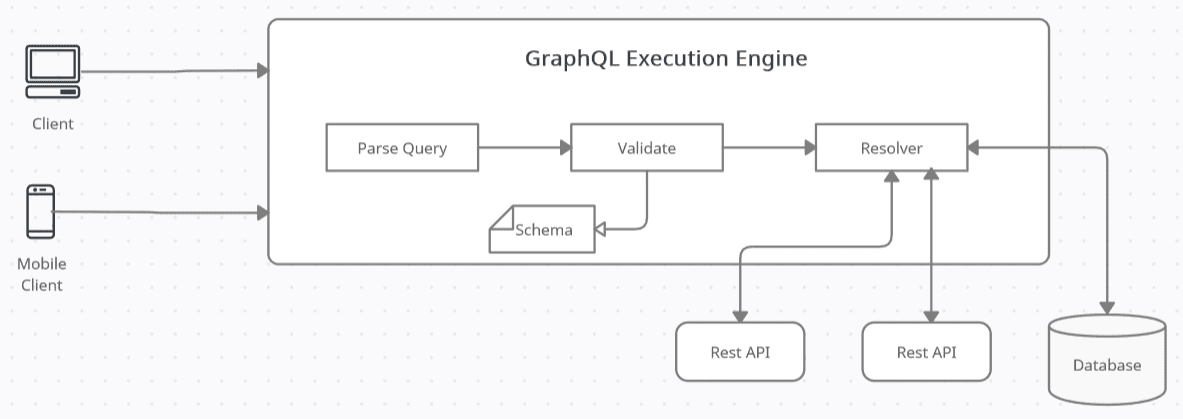
Each GraphQL query passes through three phases: parse, validate and execute. In the parse phase, the GraphQL query is tokenized and parsed into a representation known as an abstract syntax tree. In the validation phase, the graphical query is validated against the schema as shown in Figure 1.

Image showing the GraphQL execution engine

Figure 1: GraphQL execution

Finally, in the execute phase, the GraphQL runtime walks through the abstract syntax tree from the tree’s root, retrieves and aggregates the results, and sends the data back to the GraphQL client as JSON.

GraphQL vs. REST

Take a quick look at the differences between GraphQL and REST:

  • Unlike REST, which may need multiple API calls to obtain the data you want, GraphQL exposes just one endpoint you can use to get the information you need.
  • REST only works with HTTP, while GraphQL does not need HTTP.
  • Unlike REST, which allows you to use any HTTP verb, GraphQL enables you to use only the HTTP POST verb.
  • In REST, the API specifies the request and response. On the contrary, in GraphQL, the API defines the resources accessible, and the clients or consumers can request exactly the data they need from the API.
  • When working with REST, the server determines the size of the resource. On the contrary, with GraphQL, the API specifies the accessible resources, and the client requests just what it needs.
  • REST and GraphQL are both platform and language-neutral, and both can return JSON data.

Goals of GraphQL: What Problem Does It Solve?

There are several downsides of REST:

  • Over-fetching – this implies your REST API sends you more data than you need
  • Under-fetching – this implies your REST API sends you less data than you need
  • Multiple requests – requiring multiple requests to get the data you need
  • Multiple round trips – multiple requests required to complete an execution before you can proceed

Over-fetching and under-fetching are two of the common problems you would often encounter when working with REST APIs. This is explained in more detail in the next section.

The Problem of Under-Fetching and Over-Fetching Explained

Here is a typical example of REST endpoints for a typical application that manages blog posts.

GET /blogposts
GET /blogposts/{blogPostId}
GET /authors
GET /authors/{authorId}

To aggregate the data, you will have to make several calls to the endpoints shown here. Note that a request to the /blogposts endpoint would fetch the list of blogposts together with authorId, but it will not return author data. You need to make a call to /authors/{authorId} multiple times to get author details of the authors. This problem is known as under-fetching since your API payload contains less data than you need. You can take advantage of Backend for Frontend or the Gateway Aggregation pattern to solve this problem. Still, in either case, you will need multiple calls to the API endpoints.

On the contrary, your API payload might be too verbose as well. For example, you might want to know only details of the blogposts by calling the /blogposts endpoint, but your payload will also contain authorId. This problem is known as over-fetching, which implies that your API payload comprises more data than you need, hence consuming more network bandwidth. Here’s where GraphQL comes to the rescue.

Building Blocks of GraphQL

The main building blocks of GraphQL comprise schemas and types.

Schema

In GraphQL, there is just one endpoint. This endpoint provides a schema used to inform API consumers about the functionality available for clients to consume, i.e., what data they may expect and what actions they can perform. A Schema in GraphQL is a class that extends the Schema class of the GraphQL.Types namespace.

GraphQL has three primary operations: Query for reading data, Mutation for writing data, and Subscription for receiving real-time updates. A schema contains Query, Mutation, and a Subscription..

  • Query – In GraphQL, you can take advantage of queries for fetching or consuming data efficiently. The consumer or the client can mention the field or fields it needs instead of getting data for all the fields from a particular type. The client can only consume the fields that the API has exposed.
  • Mutation – In GraphQL, mutations are used to add, modify, or delete data. The client can only take advantage of the mutations that the schema has exposed to modify the data. In other words, a GraphQL client cannot manipulate data exposed by the API unless there is an appropriate mutation available.
  • Subscriptions – In GraphQL, subscriptions allow a server to send data to its clients, notifying them when events occur. Subscriptions support event-driven architectures, and they use WebSockets to provide real-time notifications.

GraphQL Object Types

One of the essential components of GraphQL schema is the object type, used to describe the kind of item that may be retrieved through your API. Object Types in GraphQL are represented using GraphQL.Types.ObjectGraphType class and contain fields and methods.

Implementing a GraphQL API in ASP.NET Core

Now leverage all learned thus far to build an application that uses GraphQL for performing CRUD operations.

Getting Started: The Solution Structure

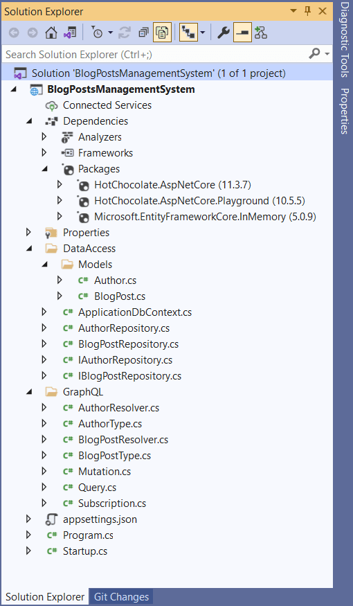
Figure 2 below illustrates the solution structure of the completed application.

Image showing the completed application

Figure 2: Application structure

As you can see, there is only one project in the Solution for the sake of simplicity. The DataAccess and GraphQL solution folders are under the root of the project. The Models solution folder is under the DataAccess solution folder. So, when this project is compiled, the following three libraries will be generated:

  • BlogPostsmanagementSystem.dll
  • BlogPostsManagementSystem.DataAccess.dll
  • BlogPostsManagementSystem.DataAccess.Models.dll

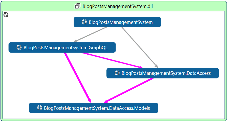
To help understand the organization of your code, including the dependencies, you can take advantage of CodeMaps in Visual Studio. Figure 3 below shows the CodeMap for this solution generated in Visual Studio 2019.

Image showing the codemaps

Figure 3: Organization of Code and Dependencies as Viewed using CodeMaps

Steps to build a GraphQL API in ASP.NET Core 5

To build the application discussed in this article, follow these steps:

  1. Create a new ASP.NET Core 5 application
  2. Install the NuGet Packages
  3. Create the Models
  4. Create the Data Context
  5. Register the Data Context
  6. Create the Repositories
  7. Add Services to the Container
  8. Build the GraphQL Schema
  9. Query
  10. Mutation
  11. Subscription
  12. Create the Resolvers
  13. Configure the GraphQL Middleware

Create a new ASP.NET Core 5 Application

First off, create a new ASP.NET Core 5 project. To do this, execute the following command at the shell:

dotnet new web -f net5.0 --no-https --name BlogPostsManagementSystem

When you execute the above command, a new ASP.NET Core 5 project without HTTPS support will be created in the current directory.

You can now take advantage of Visual Studio 2019 to open the project and make changes as needed. You’ll use this project in the sections that follow.

Install the NuGet Packages

In this example, you’ll take advantage of HotChocolate for working with GraphQL. Hot Chocolate is an open-source .NET GraphQL platform that adheres to the most current GraphQL specifications. It serves as a wrapper around the GraphQL library, making building a full-fledged GraphQL server easier.

HotChocolate is very simple to set up and configure and removes the clutter from creating GraphQL schemas. You can take advantage of HotChocolate to create a GraphQL layer on top of your existing application layer.

Since support for GraphQL is not in-built in ASP.NET Core, you’ll need to install the necessary NuGet packages via the NuGet Package Manager or the NuGet Package Manager Console.

You’ll need to install the following packages:

HotChocolate.AspNetCore
HotChocolate.AspNetCore.Playground
Microsoft.EntityFrameworkCore.InMemory

To do this, run the following commands at the NuGet Package Manager Console Window:

Install-Package HotChocolate.AspNetCore
Install-Package HotChocolate.AspNetCore.Playground
Install-Package Microsoft.EntityFrameworkCore.InMemory

Alternatively, you can install these packages by executing the following commands at the shell:

dotnet add package HotChocolate.AspNetCore
dotnet add package HotChocolate.AspNetCore.Playground
dotnet add package Microsoft.EntityFrameworkCore.InMemory

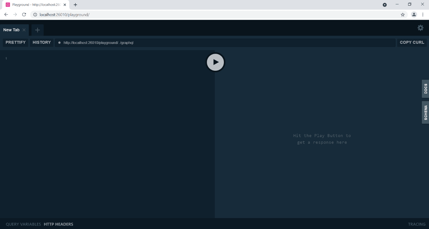
Run the application now, then add /playground to the URL to view the playground. . Here’s how the output will look in the web browser.

A screenshot of a running the application

Figure 4: Output from web browser

Create the Models

Create a solution folder called DataAccess at the root of the project. Create another solution folder inside the DataAccess folder called Models; this is where the entity classes will go.

To make things simple, you’ll use two model classes in this example named Author and BlogPost. Select your project in the Solution Explorer Window, right-click and select Add -> New Folder. Inside this folder, create two .cs files named Author.cs and BlogPost.cs with the following content:

Author.cs

using HotChocolate;
using HotChocolate.Types;
namespace BlogPostsManagementSystem.DataAccess.Models
{
    public class Author
    {
        [GraphQLType(typeof(NonNullType<IdType>))]
        public int Id { get; set; }
        [GraphQLNonNullType]
        public string FirstName { get; set; }
        [GraphQLNonNullType]
        public string LastName { get; set; }
    }
}

BlogPost.cs

using HotChocolate;
using HotChocolate.Types;
namespace BlogPostsManagementSystem.DataAccess.Models
{
    public class BlogPost
    {
        public int Id { get; set; }
        [GraphQLType(typeof(NonNullType<StringType>))]
        public string Title { get; set; }
        [GraphQLNonNullType]
        public int AuthorId { get; set; }
    }
}

The BlogPost class contains a reference to the Author class. Hence a BlogPost can be written by only one author, but an author can write many blog posts.

Build the DataContext

This example takes advantage of Entity Framework Core (in-memory) to work with data. Create a class called ApplicationDbContext inside the DataAccess solution folder of your project and write the following code in it:

ApplicationDbContext.cs

using BlogPostsManagementSystem.DataAccess.Models;
using Microsoft.EntityFrameworkCore;
namespace BlogPostsManagementSystem.DataAccess
{
    public class ApplicationDbContext : DbContext
    {
        public ApplicationDbContext(DbContextOptions
        <ApplicationDbContext> options) : base(options)
        {
        }
        public DbSet<Author> Authors { get; set; }
        public DbSet<BlogPost> BlogPosts { get; set; }
        protected override void OnModelCreating
        (ModelBuilder modelBuilder)
        {
            Author author1 = new Author
            {
                Id = 1,
                FirstName = "Joydip",
                LastName = "Kanjilal"
            };
            Author author2 = new Author
            {
                Id = 2,
                FirstName = "Steve",
                LastName = "Smith"
            };
            Author author3 = new Author
            {
                Id = 3,
                FirstName = "Anand",
                LastName = "Narayanaswamy"
            };
            modelBuilder.Entity<Author>().HasData(
            author1, author2, author3);  
            modelBuilder.Entity<BlogPost>().HasData(
                new BlogPost
                {
                    Id = 1,
                    Title = "Introducing C# 10.0",
                    AuthorId = 1
                },
                new BlogPost
                {
                    Id = 2,
                    Title = "Introducing Entity Framework 
                    Core",
                    AuthorId = 2
                },
                new BlogPost
                {
                    Id = 3,
                    Title = "Introducing Kubernetes",
                    AuthorId = 1
                },
                new BlogPost
                {
                    Id = 4,
                    Title = "Introducing Machine Learning",
                    AuthorId = 2
                },
                new BlogPost
                {
                    Id = 5,
                    Title = "Introducing DevSecOps",
                    AuthorId = 3
                }
                );
        }
    }
}

Register a Data Context Factory

Now that the data context is ready, you should register it. However, you’ll register a DbContextFactory in lieu of registering a DbContext instance since it would allow for easy creation of DbContext instances in the application when needed.

You might often want to perform multiple units-of-work within a single HTTP request. In such cases, you can use the AddDbContextFactory method to register a factory (in the ConfigureServices method of the Startup class) for creating DbContext instances. Then you can leverage constructor injection to access the factory in your application.

The following code snippet illustrates how you can take advantage of the AddDbContextFactory method to register a DbContextFactory instance:

services.AddDbContextFactory<ApplicationDbContext>(
options => options.UseInMemoryDatabase("BlogsManagement"));

The above code informs Entity Framework Core to create an in-memory database named BlogsManagement.

Create the Repositories

Create an interface named IAuthorRepository in a file called IAuthorRepository.cs inside the DataAccess solution folder of your project with the following code in there. Make sure the interfaces are public.

IAuthorRepository.cs

public interface IAuthorRepository
    {
        public List<Author> GetAuthors();
        public Author GetAuthorById(int id);
        public Task<Author> CreateAuthor(Author author);
    }

Create another interface named IBlogPostRepository in the same folder with the following code:

IBlogRepository.cs

public interface IBlogPostRepository
    {
        public List<BlogPost> GetBlogPosts();
        public BlogPost GetBlogPostById(int id);
    }

The AuthorRepository and BlogPostRepository classes will implement the interfaces IAuthorRepository and IBlogPostRepository, respectively.

Create a file named AuthorRepository.cs in the DataAccess solution folder with the following code:

AuthorRepository.cs

using BlogPostsManagementSystem.DataAccess.Models;
using Microsoft.EntityFrameworkCore;
using System.Collections.Generic;
using System.Linq;
using System.Threading.Tasks;
namespace BlogPostsManagementSystem.DataAccess
{
    public class AuthorRepository : IAuthorRepository
    {
        private readonly IDbContextFactory
            <ApplicationDbContext> _dbContextFactory;
        public AuthorRepository(IDbContextFactory
            <ApplicationDbContext> dbContextFactory)
        {
            _dbContextFactory = dbContextFactory;
            using (var _applicationDbContext = 
                _dbContextFactory.CreateDbContext())
            {
                _applicationDbContext.Database
                .EnsureCreated();
            }
        }
        public List<Author> GetAuthors()
        {
            using (var applicationDbContext = 
                _dbContextFactory.CreateDbContext())
            {
                return applicationDbContext.Authors.ToList();
            }
        }
        public Author GetAuthorById(int id)
        {
            using (var applicationDbContext = 
                _dbContextFactory.CreateDbContext())
            {
                return applicationDbContext.Authors.
                SingleOrDefault(x => x.Id == id);
            }
        }
        public async Task<Author> CreateAuthor(Author author)
        {
            using (var applicationDbContext = 
                _dbContextFactory.CreateDbContext())
            {
                await applicationDbContext.Authors
                .AddAsync(author);
                await applicationDbContext.SaveChangesAsync();
                return author;
            }
        }
    }
}

Inside the same solution folder, create a file named BlogPostRepository.cs. Replace the default generated code using the following code:

BlogPostRepository.cs

using BlogPostsManagementSystem.DataAccess.Models;
using Microsoft.EntityFrameworkCore;
using System.Collections.Generic;
using System.Linq;
namespace BlogPostsManagementSystem.DataAccess
{
    public class BlogPostRepository : IBlogPostRepository
    {
        private readonly IDbContextFactory
            <ApplicationDbContext> _dbContextFactory;
        public BlogPostRepository(IDbContextFactory
            <ApplicationDbContext> dbContextFactory)
        {
            _dbContextFactory = dbContextFactory;
            using (var applicationDbContext =
                _dbContextFactory.CreateDbContext())
            {
                applicationDbContext.Database
                .EnsureCreated();
            }
        }
        public List<BlogPost> GetBlogPosts()
        {
            using (var applicationDbContext =
                _dbContextFactory.CreateDbContext())
            {
                return applicationDbContext
                .BlogPosts.ToList();
            }
        }
        public BlogPost GetBlogPostById(int id)
        {
            using (var applicationDbContext =
                _dbContextFactory.CreateDbContext())
            {
                return applicationDbContext.BlogPosts
                    .SingleOrDefault(x => x.Id == id);
            }
        }
    }
}

Add Services to the Container

You should now add the following services in the ConfigureServices method of the Startup class so that you can take advantage of dependency injection to access instances of these types.

services.AddScoped<IAuthorRepository, AuthorRepository>();
services.AddScoped<IBlogPostRepository, BlogPostRepository>();

Build the GraphQL Schema

A GraphQL Schema comprises the following:

  • Query
  • Mutations
  • Subscriptions

Since GraphQL is not bound to any language or framework, it is not adept at understanding the CLR classes, i.e., C# POCO classes. In GraphQL, types are used to specify the fields of the domain classes you would like to expose. You’ll now create two classes, namely AuthorType in a file named AuthorType.cs and another class named BlogPostType in a file called BlogPostType.cs.

To create a type in GraphQL, you should create a class that extends ObjectGraphType<T> and pass your entity type as an argument. You should also register the properties of the class as Field types so that GraphQL can recognize this type.

Create your GraphQL folder, then create the following two classes in the files AuthorType.cs and BlogPostType.cs , respectively inside the folder.

AuthorType.cs

using BlogPostsManagementSystem.DataAccess.Models;
using HotChocolate.Types;
namespace BlogPostsManagementSystem.GraphQL
{
    public class AuthorType : ObjectType<Author>
    {
        protected override void Configure(IObjectTypeDescriptor<Author> descriptor)
        {
            descriptor.Field(a => a.Id).Type<IdType>();
            descriptor.Field(a => 
            a.FirstName).Type<StringType>();
            descriptor.Field(a => 
            a.LastName).Type<StringType>();
            descriptor.Field<BlogPostResolver>(b => 
            b.GetBlogPosts(default, default));
        }
    }
}

BlogPostType.cs

using BlogPostsManagementSystem.DataAccess.Models;
using HotChocolate.Types;
namespace BlogPostsManagementSystem.GraphQL
{
    public class BlogPostType : ObjectType<BlogPost>
    {
        protected override void 
        Configure(IObjectTypeDescriptor<BlogPost> descriptor)
        {
            descriptor.Field(b => b.Id).Type<IdType>();
            descriptor.Field(b => b.Title).Type<StringType>();
            descriptor.Field(b => b.AuthorId).Type<IntType>();
            descriptor.Field<AuthorResolver>(t => 
            t.GetAuthor(default, default));
        }
    }
}

Query

You also need a class that would fetch author and blog post-related data. To do this, create a file called AuthorQuery.cs with the following content inside.

Query.cs

using BlogPostsManagementSystem.DataAccess;
using BlogPostsManagementSystem.DataAccess.Models;
using HotChocolate;
using HotChocolate.Subscriptions;
using System.Collections.Generic;
using System.Threading.Tasks;
namespace BlogPostsManagementSystem.GraphQL
{
    public class Query
    {
        public async Task<List<Author>> 
        GetAllAuthors([Service] 
        IAuthorRepository authorRepository,
        [Service] ITopicEventSender eventSender)
        {
            List<Author> authors = 
            authorRepository.GetAuthors();
            await eventSender.SendAsync("ReturnedAuthors", 
            authors);
            return authors;
        }
        public async Task<Author> GetAuthorById([Service]
        IAuthorRepository authorRepository,
        [Service] ITopicEventSender eventSender, int id)
        {
            Author author = 
            authorRepository.GetAuthorById(id);
            await eventSender.SendAsync("ReturnedAuthor", 
            author);
            return author;
        }
        public async Task<List<BlogPost>> 
        GetAllBlogPosts([Service] IBlogPostRepository 
        blogPostRepository,
        [Service] ITopicEventSender eventSender)
        {
            List<BlogPost> blogPosts = 
            blogPostRepository.GetBlogPosts();
            await eventSender.SendAsync("ReturnedBlogPosts", 
            blogPosts);
            return blogPosts;
        }
        public async Task<BlogPost> GetBlogPostById([Service] 
        IBlogPostRepository blogPostRepository,
        [Service] ITopicEventSender eventSender, int id)
        {
            BlogPost blogPost = 
            blogPostRepository.GetBlogPostById(id);
            await eventSender.SendAsync("ReturnedBlogPost",
            blogPost);
            return blogPost;
        }
    }
}

Mutation

GraphQL uses mutation to allow the clients or consumers of an API to add, remove or modify data on the servers. You will need a query type to read data – this was discussed earlier.

Create a class called Mutation in a file named Mutation.cs inside the GraphQL solution folder and add the following code:

Mutation.cs

using BlogPostsManagementSystem.DataAccess;
using BlogPostsManagementSystem.DataAccess.Models;
using HotChocolate;
using HotChocolate.Subscriptions;
using System.Threading.Tasks;
namespace BlogPostsManagementSystem.GraphQL
{
    public class Mutation
    {
        public async Task<Author> CreateAuthor([Service] 
        AuthorRepository authorRepository,
        [Service] ITopicEventSender eventSender, int id,
        string firstName,string lastName)
        {
            var data = new Author
            {
                Id = id,
                FirstName = firstName,
                LastName = lastName
            };
            var result = await 
            authorRepository.CreateAuthor(data);
            await eventSender.SendAsync("AuthorCreated", 
            result);
            return result;
        }
    }
}

Subscription

You can take advantage of subscriptions in GraphQL to integrate real-time functionality in your GraphQL applications. Subscriptions enable servers to send data to subscribed clients to notify them when an event occurs. Subscriptions use WebSockets to allow clients to subscribe to notifications emails in real-time. The server executes the query again and then sends the updated results to the subscribed event.

Now, create a class named Subscription in a file called Subscription.cs and replace the default code with the following:

Subscription.cs

using BlogPostsManagementSystem.DataAccess.Models;
using HotChocolate;
using HotChocolate.Execution;
using HotChocolate.Subscriptions;
using HotChocolate.Types;
using System.Collections.Generic;
using System.Threading;
using System.Threading.Tasks;
namespace BlogPostsManagementSystem.GraphQL
{
    public class Subscription
    {
        [SubscribeAndResolve]
        public async ValueTask<ISourceStream<Author>> 
        OnAuthorCreated([Service] 
        ITopicEventReceiver eventReceiver,
            CancellationToken cancellationToken)
        {
            return await eventReceiver.SubscribeAsync
            <string, Author>("AuthorCreated", 
            cancellationToken);
        }
        [SubscribeAndResolve]
        public async ValueTask<ISourceStream
        <List<Author>>> OnAuthorsGet([Service] 
        ITopicEventReceiver eventReceiver,
           CancellationToken cancellationToken)
        {
            return await eventReceiver.SubscribeAsync<string, 
            List<Author>>("ReturnedAuthors", 
            cancellationToken);
        }
        [SubscribeAndResolve]
        public async ValueTask<ISourceStream<Author>> 
        OnAuthorGet([Service] ITopicEventReceiver 
        eventReceiver, CancellationToken cancellationToken)
        {
            return await eventReceiver.SubscribeAsync<string, 
            Author>("ReturnedAuthor", cancellationToken);
        }
        [SubscribeAndResolve]
        public async ValueTask<ISourceStream<BlogPost>> 
        OnBlogPostsGet([Service] ITopicEventReceiver 
        eventReceiver, CancellationToken cancellationToken)
        {
            return await eventReceiver.SubscribeAsync<string, 
            BlogPost>("ReturnedBlogPosts", cancellationToken);
        }
        [SubscribeAndResolve]
        public async ValueTask<ISourceStream<BlogPost>> 
        OnBlogPostGet([Service] ITopicEventReceiver 
        eventReceiver, CancellationToken cancellationToken)
        {
            return await eventReceiver.SubscribeAsync<string, 
            BlogPost>("ReturnedBlogPost", cancellationToken);
        }
    }
}

Create the Resolvers

A resolver is a function responsible for populating data for one field of your schema. In other words, it is a function that resolves the value of a type of field within a schema. Resolvers can return objects and scalars such as Strings, Numbers, or Booleans. You can define how it populates the data, including fetching data from a third-party API or back-end database.

Create a class called AuthorResolver in a file named AuthorResolver.cs inside the GraphQL solution folder with the following code:

AuthorResolver.cs

using BlogPostsManagementSystem.DataAccess;
using BlogPostsManagementSystem.DataAccess.Models;
using HotChocolate;
using HotChocolate.Resolvers;
using System.Linq;
namespace BlogPostsManagementSystem.GraphQL
{
    public class AuthorResolver
    {
        private readonly IAuthorRepository _authorRepository;
        public AuthorResolver([Service] IAuthorRepository 
        authorService)
        {
            _authorRepository = authorService;
        }
        public Author GetAuthor(BlogPost blog, 
        IResolverContext ctx)
        {
            return _authorRepository.GetAuthors().Where
            (a => a.Id == blog.AuthorId).FirstOrDefault();
        }
    }
}

Create another class named BlogPostResolver in a file called BlogPostResolver.cs with the following code:

BlogPostResolver.cs

using BlogPostsManagementSystem.DataAccess;
using BlogPostsManagementSystem.DataAccess.Models;
using HotChocolate;
using HotChocolate.Resolvers;
using System.Collections.Generic;
using System.Linq;
namespace BlogPostsManagementSystem.GraphQL
{
    public class BlogPostResolver
    {
        private readonly IBlogPostRepository 
        _blogPostRepository;
        public BlogPostResolver([Service] 
        IBlogPostRepository blogPostRepository)
        {
            _blogPostRepository = blogPostRepository;
        }
        public IEnumerable<BlogPost> GetBlogPosts(
        Author author, IResolverContext ctx)
        {
            return _blogPostRepository.GetBlogPosts()
            .Where(b => b.AuthorId == author.Id);
        }
    }
}

Configuring the GraphQL Middleware

Write the following code in the ConfigureServices method of the Startup class to add GraphQLServer to the container:

services.AddGraphQLServer();

A GraphQL server can expose data via GraphQL API endpoints so that the same data can be consumed by the clients (mobile clients, web clients, etc.) or the consumers of the API.

Next, write the following code in the Configure method of the Startup class to configure the GraphQL endpoint:

public void Configure(IApplicationBuilder app, IWebHostEnvironment env)
        {
            if (env.IsDevelopment())
            {
                app.UseDeveloperExceptionPage();
                app.UsePlayground(new PlaygroundOptions
                {
                    QueryPath = "/graphql",
                    Path = "/playground"
                });
            }
            app.UseWebSockets();
            app
                .UseRouting()
                .UseEndpoints(endpoints =>
                {
                    endpoints.MapGraphQL();
                });
        }
    }

At this moment, your ConfigureServices method should look like this:

public void ConfigureServices(IServiceCollection services)
        {
            services.AddDbContextFactory<ApplicationDbContext>(
            options => options.UseInMemoryDatabase("BlogsManagement"));
            services.AddInMemorySubscriptions();
            services.AddScoped<IAuthorRepository, 
                AuthorRepository>();
            services.AddScoped<IBlogPostRepository, 
                BlogPostRepository>();
            services
            .AddGraphQLServer()
            .AddType<AuthorType>()
            .AddType<BlogPostType>()
            .AddQueryType<Query>()
            .AddMutationType<Mutation>()
            .AddSubscriptionType<Subscription>();
        }

You should include the following namespaces in the Startup.cs file:

using BlogPostsManagementSystem.DataAccess;
using BlogPostsManagementSystem.GraphQL;
using HotChocolate.AspNetCore;
using HotChocolate.AspNetCore.Playground;
using Microsoft.AspNetCore.Builder;
using Microsoft.AspNetCore.Hosting;
using Microsoft.EntityFrameworkCore;
using Microsoft.Extensions.DependencyInjection;
using Microsoft.Extensions.Hosting;

Here’s the complete source code of the Startup class for your reference:

Startup.cs

using BlogPostsManagementSystem.DataAccess;
using BlogPostsManagementSystem.GraphQL;
using HotChocolate.AspNetCore;
using HotChocolate.AspNetCore.Playground;
using Microsoft.AspNetCore.Builder;
using Microsoft.AspNetCore.Hosting;
using Microsoft.EntityFrameworkCore;
using Microsoft.Extensions.DependencyInjection;
using Microsoft.Extensions.Hosting;
namespace BlogPostsManagementSystem
{
    public class Startup
    {
        public void ConfigureServices(IServiceCollection services)
        {
            services.AddDbContextFactory<ApplicationDbContext>(
            options => options.UseInMemoryDatabase("BlogsManagement"));
            services.AddInMemorySubscriptions();
            services.AddScoped<IAuthorRepository, 
                AuthorRepository>();
            services.AddScoped<IBlogPostRepository, 
                BlogPostRepository>();
            services
            .AddGraphQLServer()
            .AddType<AuthorType>()
            .AddType<BlogPostType>()
            .AddQueryType<Query>()
            .AddMutationType<Mutation>()
            .AddSubscriptionType<Subscription>();
        }
        public void Configure(IApplicationBuilder app, IWebHostEnvironment env)
        {
            if (env.IsDevelopment())
            {
                app.UseDeveloperExceptionPage();
                app.UsePlayground(new PlaygroundOptions
                {
                    QueryPath = "/graphql",
                    Path = "/playground"
                });
            }
            app.UseWebSockets();
            app
                .UseRouting()
                .UseEndpoints(endpoints =>
                {
                    endpoints.MapGraphQL();
                });
        }
    }
}

GraphQL in Action!

Now it’s time to execute GraphQL queries using HotChocolate. Run the application, remembering to have /playground in the URL.

Query

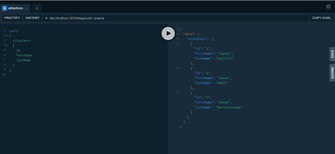
Here’s an example of a GraphQL query you can use to get the data about all authors.

query {
  allAuthors{
    id
    firstName
    lastName
  }
}

When you execute this query, here’s how the output would look like:

Image showing the query output

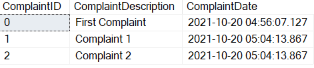
Figure 5: Query output

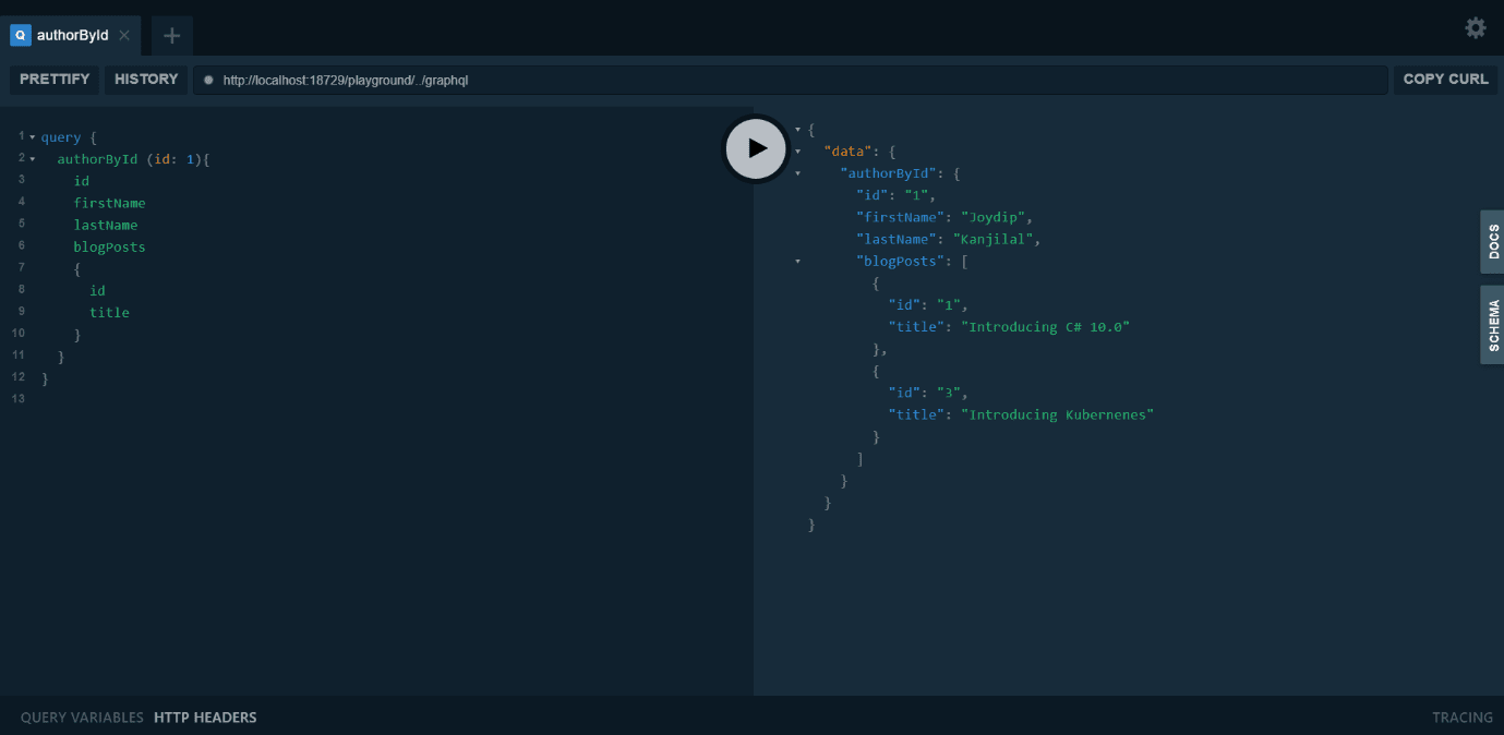
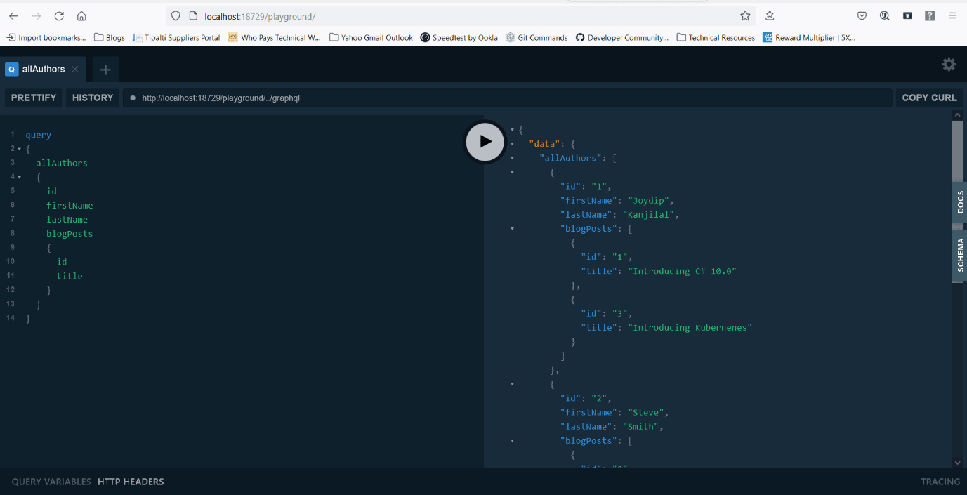
If you would like to get the data about a particular author together with the blogs they have written, you can take advantage of the following query instead.

query {
  authorById (id: 1){
    id
    firstName
    lastName
    blogPosts
    {
      id
      title
    }
  }
}

Run the above query. Figure 6 below shows the output in the Playground tool.

Image showing output of playground tool

Figure 6: Output in Playground tool
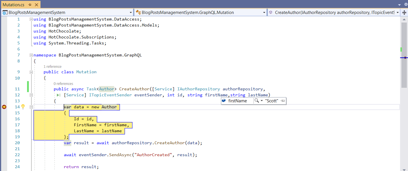
Mutation

Now write the following query to test mutation:

mutation{
  createAuthor(id: 4, firstName: "Scott", lastName: "Miller"){
    id
    firstName
    lastName
  }
}

When you run it, you’ll observe that the CreateAuthor method of your Mutation class is called. Note that the breakpoint is hit successfully.

Image showing the CreateAuthor method

Figure 7: CreateAuthor method
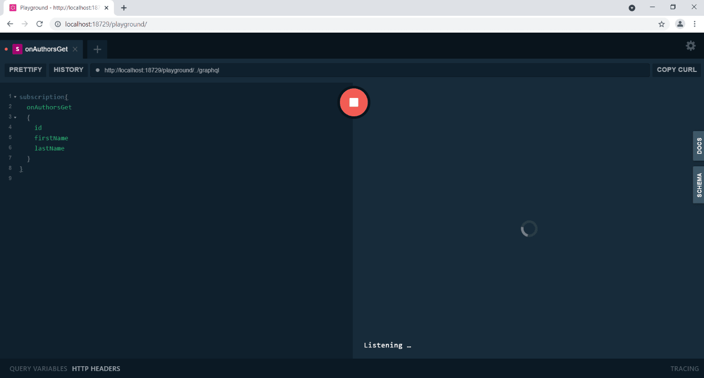
Subscription

To test Subscription, execute the application, browse to the /playground endpoint, and write the query shown below:

subscription{
  onAuthorsGet
  {
    id
    firstName
    lastName
  }
}

When you click the Execute button, the application subscribes to the OnAuthorGet event.

Image showing execute

Figure 8: Click Execute button

Next, launch the same URL in another browser window and write and execute the query shown in Figure 9.

Image showing Launch and execute the query

Figure 9: Launch and execute the query

This query will trigger the OnAuthorsGet event as shown in Figure 10.

Image showing OnAuthors event

Figure 10: The OnAuthorsGet event

Summary

GraphQL is an open-source API standard developed by Facebook that provides a powerful, flexible, and versatile alternative to REST. GraphQL supports declarative data fetching, which allows the user to specify precisely the data it needs. HotChocolate, an implementation of GraphQL, can be used to create GraphQL servers in ASP.NET Core.

If you liked this article, you might also like Building and consuming GraphQL API in ASP.NET Core 3.1 – Simple Talk (red-gate.com).

The post Building and consuming GraphQL API in ASP.NET Core 5 appeared first on Simple Talk.


from Simple Talk https://ift.tt/3vu75NG
via