Monday, December 19, 2022

SQL Server 2022: How Auto-Drop Statistics Work

Auto-Create statistics is a well-known feature critical for the database performance. When one statistic is auto created, changing the table structure is not blocked by the presence of the statistic. An auto-created statistics is also dropped automatically when a schema change happens.

On the other hand, if the statistic is created by the user, any schema change will be blocked by the presence of the statistic.

The Auto-Drop setting on a statistic is a new SQL Server 2022 feature to change this behaviour. If a user created statistic is set with the auto-drop option, it will behave as an auto-created statistics: It will be automatically dropped if a schema change happens.

Let’s make an example using AdventureWorks2019. You can download it on https://learn.microsoft.com/en-us/sql/samples/adventureworks-install-configure?view=sql-server-ver16&tabs=ssms . Restore the backup in a SQL Server 2022.

Demonstration

Our example will use the table Production.Product and focus on the field ListPrice. Let’s see a sequence of steps for this demonstration.

1) Drop the constraint CK_product_listprice, otherwise it will block the demonstration

ALTER TABLE production.product
  DROP CONSTRAINT ck_product_listprice 

2) Check the existing statistics. You will not find anyone related to ListPrice field.

3) Execute the following query:

SELECT *
FROM   production.product
WHERE  listprice = 10 

3) Check the statistics again. A new statistic was automatically created for the ListPrice field.

Interface gráfica do usuário, Texto, Aplicativo Descrição gerada automaticamente

4) Alter the column ListPrice.

ALTER TABLE production.product
  ALTER COLUMN listprice NUMERIC(18, 2) 

5) Check the statistics again. SQL Server will drop the auto-created statistic automatically.

Texto Descrição gerada automaticamente

6) Create a new statistics on the field ListPrice. It’s a user created statistics.

CREATE STATISTICS [mystats] ON production.product(listprice) 

Texto Descrição gerada automaticamente

7) Try to change the schema again. An error will happen.

ALTER TABLE production.product
  ALTER COLUMN listprice MONEY 

Interface gráfica do usuário, Texto, Aplicativo Descrição gerada automaticamente com confiança média

8) Drop the user created statistic

DROP statistic production.product.mystats 

9) Create the statistics again, this time using the auto-drop option.

CREATE statistics [mystats] ON production.product(listprice) WITH auto_drop=ON 

10) Try to change the schema again. This time it will work and the statistics mystats will be dropped

ALTER TABLE production.product
  ALTER COLUMN listprice MONEY 

Checking which statistics have the auto-drop option

A simple query can help identify which statistics have the auto-drop option and which ones doesn’t:

SELECT object_id,
       NAME,
       auto_drop
FROM   sys.stats 

Conclusion

This is a simple new feature, but it can help in some scenarios of version control and automated deployment for database schemas.


The post SQL Server 2022: How Auto-Drop Statistics Work appeared first on Simple Talk.


from Simple Talk https://ift.tt/YRh26EM
via

Resolving to Write in the New Year

It is almost New Year’s Day, that time when the optimistic at heart start thinking about making changes in their life on that magical day that ends the year. After the glorious gluttony-fest that has only recently ended in many cultures, it does feel like a great time to start.

If you have your life/work balance perfected and don’t work or read blogs in months with holidays, maybe you are seeing this later. Either way, you may have been coming up with well-meaning resolutions to eat better, exercise more, be nice to even the most annoying in your life, etc. or you are struggling to keep them. Let’s be honest; resolutions are so very hard because there are always reasons to eat delicious unhealthy foods on the couch while grousing about your neighbor that mows their lawn at 6 AM on Monday morning when you are trying to sleep a few more hours.

I want to offer you a different challenge, writing more. Assuming you have read this far, past the title and the previous sentence, I am assuming I have your attention. As the editor of Simple-Talk, I am here to offer you a few deals. First, you send me tips on how to eat better and exercise more while being constantly busy, and I will do what I can to help you with writing.

  • Put your ideas in the comments, and the best ones will share a belated holiday gift from me. One of 5 $10 Starbucks or Amazon gift cards (where allowed). If your comment is good enough, you might just get all of them!

Why should I write?

There are several reasons that you commonly hear (and most are very true.) My focus will be on technical writing, but most of the reasons I state here can be applied to non-technical things. Travel, vacations, parenting, cooking, or simply writing down your memories.

Firstly, you are helping others out by teaching them something. Even just sharing your vacation memories show others’ ideas for their vacations. Technical writing takes this to another level because the topics are about our vocations. Selfishly, this also serves to get your name out there and can help you expand your future career horizons. I have known so many people who have started out writing as a relative newbie and are now known worldwide, simply by starting out blogging and sharing their knowledge. For now, just ignore the prospects of being world famous and writing your eighth query tuning book from your own personal yacht one day because it is very unlikely.

The best value in writing is something you learned about in grade school…writing stuff down helps you remember things. In addition to the near-time values of talking notes, I will give you a quick realization that you will not want to hear. Brace yourself, sit down, whatever you need to do when you hear bad news… You are getting older. And while the whole process is exhausting, with age does come wisdom. You start to see the future more clearly and understand all the mistakes you made in your life in such a way that you can actually effect some changes in your life and you reader’s lives.

But (isn’t there always some but?) while wisdom increases, it seems to take up much more space in your brain. So, while you begin to see the big picture clearly, you will forget the details of practically everything you did. Sadly, this is also when you realize “if I had only written things down.”

Sharing your knowledge with others includes sharing with your future self. Therefore you write. When you actually have to do a task you haven’t done in years, you can go to a search engine and search for your own blog. If I was looking for information on granting rights, I might type: https://www.google.com/search?q=louis+davidson+grant, and included in the first page of results is this:

Text Description automatically generated

A blog I wrote 13 years ago! So, you can not only share your knowledge with others, but you also share it with yourself.

I want to write; how do I get started?

Thank you for asking. Search for “how to start a blog,” and you will find lots of possibilities. Pick one and start it out. When you do something at work, spend an hour writing it down and publishing it. (There are caveats, like never use customer data, never repeat proprietary techniques, etc., so don’t try to say I told you to do that. It isn’t going to work!) Even writing just well enough that you can read it and understand it without knowing any context from your work/client is perfect.

But you say you just found out how something worked in an article someone else wrote? So? By no means am I suggesting you simply repeat exactly what you read, ever. On those occasions where the writer did such a great job that you can’t think of anything to add, pop it on social media and say, “Thank you!” If you use their ideas as a jumping-off point (maybe theirs was not clear enough, didn’t exactly cover exactly what you needed,) credit them in your complimentary blog and you both win.

If you don’t have any real-world topics that you could anonymize enough to blog on, consider learning something you may need someday. This is what I did when I wrote this blog on bitwise functions in SQL Server 2022. Just write about something for the learning of it.

One mistake many people make is thinking that professional looking is equated to professional quality. If you are getting started, don’t spend a ton of time trying to build a blog that is super beautiful or has a sophisticated interface. Frankly, most of your traffic is going to come from search engines and/or posting to social media sites going directly to your blogs and will never see your home page. If you can avoid a platform that has a ton of advertisements that you cannot control (this is how they make their money if you don’t wish to pay for your site), that is best, but you don’t need to spend a lot of money to have a decent looking blog.

If all else fails… ask for help

I am as big of a fan as asking for help as you might imagine. I will wander around city streets lost as can be if my device won’t give me directions. But the best thing I have ever done was a friend 20 years ago about blogging. They sent me to a blog site named sqlblog dot com and I really got going with a blog (not a link because it is basically extinct now, and not to be confused with sqlblog.org, which is Aaron Bertrand’s site.)

If you need help finding a home for your blogs, feel free to drop me an email at editor@simple-talk.com and I will try to give you any help I can (time permitting of course!)

So, get to commenting and giving me miracle health cures in the comments. I promise that one winner will be completely picked based on the outlandishness of the suggestion!


The post Resolving to Write in the New Year appeared first on Simple Talk.


from Simple Talk https://ift.tt/aAQNqgJ
via

Monday, December 12, 2022

What’s new on Power BI DataMarts UI

I wrote an article about Power BI Datamarts which was released together the feature, on the exact moment it was being announced in a conference. Of course, this feature has being evolved since that time.

I would emphasize the performance. The general UI performance seems way better than when it was first released. Let’s talk about some more news on the Power BI Datamarts, specially on the UI.

It’s easier to change the datamarts name

By clicking on the top of the window, on the datamart name, we can easily change the datamart name. When it was first created, the name was default and the datamart had to be renamed later.

Texto Descrição gerada automaticamente com confiança baixa

We can save queries

A very welcome new feature for exploratory analysis is the possibility to save the queries we built. Either Visual Queries or SQL Queries, we can save and name them.

Interface gráfica do usuário, Texto, Aplicativo, Email Descrição gerada automaticamente

Interface gráfica do usuário, Texto, Aplicativo Descrição gerada automaticamente

Apparently, we can’t delete the queries yet, only save, but one problem at a time.

SQL Queries in a different place

The SQL Queries are not in the lower tabs anymore, but in a top button, a bit more hidden. Probably most users prefer the visual query than the SQL Query.

Interface gráfica do usuário, Aplicativo, Word Descrição gerada automaticamente

Export to Excel in Visual Queries

When I first wrote about Power BI datamarts, the Open in Excel option was only available for SQL Queries, not for Visual Queries.

Of course, it was just a matter of time for the Export to Excel be included in the Visual Query as well.

Power BI Desktop connection to SQL

When we try to connect from Power BI desktop to the datamart, now we have the option to choose if we would like to connect to the azure SQL behind the scenes or make a live connection to the Power BI Analysis Services, connecting to the model.

Interface gráfica do usuário, Texto, Aplicativo, Email Descrição gerada automaticamente

Datamart Connectivity

Using Power BI Desktop, you can connect either to the Dataset or the Datamart and the result will be the same: It appears as a live connection to Analysis Services, the Power BI underlying engine, in a simplified way.

In order to build a composite model, mixing the data from the data mart and other sources, you need the use of a preview feature: DirectQuery for PBI datasets and AS

Once this preview feature is enabled in Power BI Desktop, you can convert the Live connection in DirectQuery by clicking on the button Make Changes to this model.

The message will request you to click on the button Add a local model. This is exactly the difference between the Live connection and a composite model: The Live connection has no local model, is  Live, while a composite model has a local model where the connections to the source are defined as DirectQuery or Import.

Interface gráfica do usuário Descrição gerada automaticamente


Conclusion

In my humble opinion, the feature was already so good when it was released that it’s receiving only few adjustments, but very welcome.


The post What’s new on Power BI DataMarts UI appeared first on Simple Talk.


from Simple Talk https://ift.tt/85YkXu9
via

Friday, December 9, 2022

Backing up MySQL Part 8: Zmanda Backups for MySQL & Other Backup Tools

“A Backup as Revolutionary as You Are.” Ever heard that phrase before? If you did, you’re no stranger to Zmanda Recovery Manager – or ZRM for short. Zmanda Recovery Manager is a terabyte-scale backup tool helping you take MySQL backups with ease, scalability, and without downtime – today we’re telling you all about it and other backup tools specific to MySQL that you might not have heard about. Excited? We are too. Let’s go!

What Is Zmanda Recovery Manager?

As already mentioned, Zmanda Recovery Manager (or ZRM for short) is a member of the Zmanda family of products – Zmanda is famous for offering backup tools for MySQL and MariaDB. The company allows its customers to scale up without any issues (they offer a pay-as-you-go subscription model), and its tools are capable to back up terabytes of data in MySQL.

ZRM for MySQL

ZRM for MySQL solves various problems faced by MySQL DBAs:

  • The tool provides the ability to take physical, raw, and logical backups through a web-based management console – think of the tool as something similar to phpMyAdmin, but better.
  • ZRM for MySQL supports Windows.
  • ZRM for MySQL supports various backup types:
    • ZRM can be used to take logical backups (backups that back up statements that build up data.)
    • ZRM can also be used to back up data and store a binary copy of the data files – such backups are called raw backups and they generally provide a faster rate of recovery (in their documentation, Zmanda says that it’s not at all unusual to see that for the same 5GB database, the recovery time of raw backups is around 20 times faster than the recovery time concerning logical backups.)
    • ZRM provides its users with the ability to take hot and warm backups – hot backups provide us with the ability to back up a database without any impact on users while warm backups lock all of our tables for writing during the backup (nothing can be written into them until the backup is complete.) More information on how these kinds of backup operations work can be found in ZRM’s documentation.

Zmanda’s GUI lets its users choose what they want to backup, where they want their backups to be stored, and how the backups are supposed to be taken, however, before working with ZRM, users need to install it – doing so isn’t very difficult though, and if you follow the steps outlined in the video made by the team, you should be good to go.

As far as ZRM goes, though, it’s not without its flaws – one of its drawbacks is that the tool is enterprise-grade, and even though it offers its users a free trial, seasoned software engineers will tell you that enterprise-grade software, security, and backup solutions are far from the cheapest – if you don’t want to shell out thousands for a backup solution, other tools can help.

Other Backup Software for MySQL

SQL Backup and FTP

Aside from enterprise-grade weapons directed at backing our most precious data, there are other kinds of options, too.

One of those options is called SQL Backup and FTP – a solution that’s built to be very simple to use and looks like this (the image is an example provided by SQLBackupandFTP.)

As far as this tool is concerned, everything is all pretty self-explanatory:

  1. We need to connect to our MySQL server (see “Connect to MySQL Server.”)
  2. Once the server is specified, we need to specify the databases that we’re going to back up (“Select databases.”)
  3. Once that’s done, we select where we want to store the databases (“Store backups in selected destinations”), and whether we want to receive a confirmation once the backup is done (“Send confirmation.”)

If we wish, we can also schedule our backups (see “Schedule backups”), and then we need to run the backup job (click the button in the upper right corner.) Once our backup would be finished, it would be stored in the specified directory – as easy as that.

Bear in mind that while SQL Backup and FTP does what it’s advertised for and is quite powerful at its backup operations, it’s ill-equipped to handle bigger and more complex workloads – for that, you would need to turn to SQLBak.

SQLBak

SQLBak works similarly to SQL Backup and FTP, but it has a couple of extra features as well – it can take both full and incremental backups, restore backups, as well as send the confirmation of successful backups to a specified email address. The tool looks like this (image from SQLBak).

As you might be able to tell, the tool has a couple of extra features SQLBackupandFTP does not including, but not limited to giving its users the ability to specify multiple destinations the backup is going to be stored in, giving its users the ability to compress and encrypt its backups with the strongest algorithm on the market, etc.

The rest of the features is up to you to explore!

Summary

In the last blog of our backup series, we have walked you through a couple of additional backup tools available to MySQL DBAs – while some of the backup tools (ZRM) that were shown were enterprise-grade only, we have also provided a couple of well-known alternatives.

With that, our backup series is effectively over – we hope that you’ve enjoyed reading the blog, let us know what you think in the comment section down below, come back to our blog for more interesting content related to database backups, security, and performance, and until next time!

The post Backing up MySQL Part 8: Zmanda Backups for MySQL & Other Backup Tools appeared first on Simple Talk.


from Simple Talk https://ift.tt/Ecyo1Zp
via

Monday, December 5, 2022

The Good, The Bad, and Suboptimal of Sticking to What You Know

The Good

In the late 1990s, one of the world’s most popular technologies was waning. COBOL. Relational databases were starting to take over, and COBOL usage was waning. By now, you would think it was utterly dead, right? You would be wrong.

Go to a search engine and look for COBOL jobs, and you will find that not only is COBOL not dead, but according to sources like InfoWorld, it is somewhat hanging in there. While it is not exactly celebrated as modern technology, it is not in palliative care either.

Almost any technology you invest your time in will stick around for far longer than many news outlets and bloggers will make it seem. The death of the relational database has been forecast pretty much since the mid-1980s when Codd’s Rules were published, outlining what a relational database management system actually was.

It only gets louder as time passes, especially as NoSQL technologies have blossomed. If you love the language you work with now, you may be able to keep working in it forever. I have made a (please read this in a very humble tone) rather decent living writing and tuning Microsoft SQL T-SQL for the past 30 years. I very much doubt it will go away in the next 30 years time, by which I will be in (what I hope is a rocket-powered) rocking chair and watching all of the movies I have been enqueuing but rarely serving from that queue over many years.

The Suboptimal

While working in a comfortable environment (be that a language, a company, amount of travel, etc.) is desirable, resting on your laurels is rarely a good thing. Too many people go from hungry to learn to comfortable with their level of knowledge, ready to ride out the rest of their years. If you already have a date on your calendar circled for retirement in the next few years, being somewhat reticent to keep up with the latest trends may be just fine. But if you don’t fit that category, best to keep your head out of the sand.

While I have been a specialist in T-SQL for many years (and hope to remain as such for many seasons to come!), it is not the only thing I have ever done, nor do I want it to be. Even in just database technologies, there are many other platforms than Microsoft SQL Server that have value, such as MySQL, PostgreSQL, and even Oracle. Then there are things like graph and document databases and even NoSQL (not only SQL) technologies that have their place at the data storage table.

Spend a little time learning what these technologies offer (and do NOT offer!) you and your customers as a programmer. Your eyes may be opened to possibilities now and future opportunities.

The Bad

Saving the worst for last, I want to talk about the worst thing that people do (again, who aren’t just about to retire!). This is not only ignoring new technologies but refusing to learn new techniques. You can do the things you know how to do, so why learn new things?

Are all new features useful? Are the algorithms you have mastered the best? Maybe, maybe not. But I have known too many people who have their lives figured out and don’t care about new features. They can back up, restore, and check the integrity of databases. They can create a GUI, accept input, and store data in a database. Job done in version N and still works in version N+10; why care?

Where do I start? First, each release of tools and products has many new features that can improve your life. Backups get encryption, compression, and better targets than that tape drive you have used for 20 years. Integrity checks get new parameters that make things faster and less disruptive to users. Perhaps more importantly, techniques that allow you to continually check data structures while users are using the data. Don’t be that DBA that makes your company put up a banner to customers that says:”this website will be down for 18 hours a day for your convenience whenever it is up.”

There are also completely new features out there that can make your work easier. Maybe you are using interpreted code, and a new compiled version has arrived that will run 100 times faster on 1/2 the hardware. Or there is a new index type that can take your processing time from 3 hours to 3 minutes for a necessary process.

A weird problem that having a senior programmer with limited skills causes is it can drag down an entire team for years to come. When new people are interviewed, the senior person doing the interview may not realize just how skilled interviewees are, leading to stagnation in the future. They were talking about something called a document database. That isn’t even a thing, right?”

Keep up, at least somewhat

Even if your organization will never let you use some features, keep up with as much as you can. Not only are there improvements to product’s functionality, but the more significant issues tend to be security. If you spend time reading blogs and news, use a password manager of any quality, or take 10 seconds and type your passwords into https://ift.tt/ONFLAS7, you will quickly realize that security is amazingly important, and products stop updating themselves even for security eventually.

To end this article, let’s be mildly selfish for a second. It is extraordinarily rare that a person stays with the same organization for 25 years (even I left my last employer at 24 years and 9 months). Many don’t even stay 2 years. One day you may have this feeling that you want to change positions and find yourself face-to-face with a person interviewing you for your dream job.

You sit there, eye to eye, with this friendly person doing your technical interview. You have met several others who seemed very excited to hire you after meeting you. You are filled with this glorious “I got this!” feeling, fighting a smile back as you chit-chat about general topics with your technical interviewer. Then the first technical question escapes heir mouth, and that feeling changes to something a bit less optimistic. After a few more questions, you realize that your knowledge of Generic RDBMS 4.678 doesn’t even translate to the current version (10.1). Your previous co-workers who taught you most of what you know (which, it turns out, is barely enough to keep your previous situation from bursting into flames) were, to put it kindly, clueless. (This is NOT my story at all, but it is very much a true story.)

Your moment of glory flies away like a dandelion pappus on a breezy day, and you will either start learning or learn to live where you are.


The post The Good, The Bad, and Suboptimal of Sticking to What You Know appeared first on Simple Talk.


from Simple Talk https://ift.tt/6Kyz8Ug
via

Dealing with the Bits of a Binary Value in SQL Server

How you used to do it

For example, say you want to find all the read-write database using SQL Server 2022 system objects (I think this started back in 2005, in fact). You can write:

SELECT name
FROM sys.databases
WHERE is_read_only = 0
  AND name IN ('master','msdb','tempdb');

This will return those three system databases (because they still will always be read-write.) Using the old sysdatabases object, there was just a status column.

SELECT name, status
FROM   sys.sysdatabases
WHERE  name IN ('master','msdb','tempdb');

On my computer, and most likely yours, the output from this query is:

name           status
-------------- -----------
master         65544
msdb           65544
tempdb         65544

I expect that 99% of the people reading this looks at this probably would expect there to be a status table that contained the values of status. Seeing that this is a base 2 number, you may be in that 1% that thinks this might be a bitmask. but unless you have and eidetic memory, you probably don’t know what all of the bits mean.

A bitmask is a type of denormalization of values where instead of having a set of columns that have on or off values (no Null values), you encode it like:

00000101

Now the user has to figure out what bit each of the 8 bits are in the integer/binary value to determine a value. For status, you can determine if a database is read-only using the 10th place. In versions of SQL Server before 2022, this was achieved by doing something like this:

SELECT name, status & 1024 AS is_readonly
FROM   sys.sysdatabases
WHERE  name IN ('master','msdb','tempdb');

The idea is that if the 10th bit in the number is set to 1, that it AND (&) the value will return 1024 (since it will return 1024 (which is POWER(2,10)), and if it is value, it will return 0. (For the full list of bit values, check here: https://learn.microsoft.com/en-us/sql/relational-databases/system-compatibility-views/sys-sysdatabases-transact-sql?view=sql-server-ver16)

To see one that does return a match, check out the following 2 queries:

SELECT name
FROM   sys.databases
WHERE  page_verify_option_desc = 'CHECKSUM'
  AND  name IN ('master','msdb','tempdb');

SELECT name
FROM   sys.sysdatabases
WHERE  status & 65536 = 65536 
 AND name IN ('master','msdb','tempdb');

Both return three rows. Ok, so that is the basics, now lets look at some new syntax that makes this easier. For example, let’s take that 65536 value. It is 2 to the 16th power:

SELECT POWER(2,16); --returns 65536

In SQL Server 2022, there are 5 new bitwise functions that have some value. For example, finding that a bit is set is a lot easier. The functions are:

  • GET_BIT – See if a bit is set in a binary value
  • SET_BIT – Set a bit in a binary value and return the new value
  • LEFT_SHIFT, RIGHT_SHIFT – Shift all the bits left or right in a binary value
  • BIT_COUNT – count the number of bits set in a value

In our previous query of status and checksum, you could rewrite as:

SELECT name, GET_BIT(status,10) AS is_readonly,
                         GET_BIT(status,16) AS is_checksum
FROM   sys.sysdatabases
WHERE  name IN ('master','msdb','tempdb');

This returns:

name         is_readonly is_checksum
------------ -----------  -----------
master                 0            1
msdb                   0            1
tempdb                 0            1

While I am STILL never in my life going to bless a bitwise solution in the year 2022 (much less the year 2000), this does make it far less unpleasant to work with.

The rest of the bit functions are less useful in any solution I have ever seen, but they are interesting. For example:

DECLARE @value VARBINARY(64) = 0;

SET @value = SET_BIT(@value,10);

SELECT @value AS INT[

This returns:

-------------
0x00000400

Which is binary for 1024. Note that while bits may be technically implemented in SQL Server internally as bits from the left, the bit operators treat values as if they were from the right (since that maps to our typical numbering system). Now let’s set bits 1, 2, 3, and 4, then shift those bits right:

SELECT SET_BIT(SET_BIT(SET_BIT(SET_BIT(0,1),2),3),4);

This outputs 30.. which may confuse you (it did me!), there is a bit 0 also. So it is 2 + 4 + 8 + 16 = 30

Shifting 30 right 1 position:

SELECT RIGHT_SHIFT(30,1);

This outputs 15, which is now 1 + 2 + 4 + 8. Let’s shift it again:

SELECT RIGHT_SHIFT(30,2);

This is analogous to RIGHT_SHIFT(RIGHT_SHIFT(30,1),1) and returns 7. Bits fall off to the side, so, for example:

SELECT LEFT_SHIFT(RIGHT_SHIFT(30,100),100);

Returns 0, because the first set of RIGHT_SHIFT statements pushed the bits al the way off of the map. Swap the calls:

SELECT RIGHT_SHIFT(LEFT_SHIFT(30,100),100);

And wait… it still falls off and returns 0. Why? Because this is technically a 31-bit integer (the sign takes off a bit), so you lose the bits anyhow. So be careful bit shifting!

Finally, let’s look at the BIT_COUNT function. Using the 30 value, which we know is 2 + 4 + 8 + 16. Next, execute the following:

SELECT BIT_COUNT(30);

And you will see that it returns 4, telling us there are 4 bits that are 1.

Might be the bit of information you absolutely never have a valid use for, but the more you know, you may some day actually need it!


The post Dealing with the Bits of a Binary Value in SQL Server appeared first on Simple Talk.


from Simple Talk https://ift.tt/zMGTcbR
via

Saturday, December 3, 2022

Backing Up MySQL Part 7: MySQL Enterprise Backup

MySQL Enterprise Backup is a known tool for everyone inside of the world of MySQL, no matter if people dealing with the tool are enterprise (business) minded or not. The tool can be considered the flagship of MySQL’s enterprise-level offerings: it comes as a part of its Enterprise tier and costs thousands to attain: is it worth your money, and perhaps more importantly, your time? We will figure that out in this blog.

Enterprise-level Backups and the Enterprise Tier of MySQL

In case you’re not aware of it yet, the Enterprise tier of MySQL can offer people a couple of interesting features and tools, including, but not limited to firewalls, data masking and de-identification, and, of course, backup features; the Enterprise Backup tool of MySQL makes MySQL capable to perform online, hot backups of any type: no matter if they’re full, incremental, or partial.

The enterprise tier of MySQL’s offerings is an important part of their business because it offers it all: monitoring, encryption, masking, auditing, a database-related firewall (we’ve covered some of the things it does in our security-related blogs), and, of course, the Enterprise Backup capability. The former is what we’re after for this blog post, so here’s what MySQL Enterprise Backup means for you as a user:

Feature

Meaning

The ability to take multiple types of backups without sacrificing on performance

MySQL Enterprise Backup is capable of taking hot, full, partial, and incremental backups without disturbing the performance of MySQL while completing the process. For more information on the types of backups available in MySQL, refer to the documentation.

Compression and Encryption

MySQL Enterprise Backup offers the ability to encrypt backups using the industry-standard AES256 capability as well as compress them using zlib, LZ4, or LZMA.

The ability to include or exclude tables from a backup

MySQL Enterprise Backup gives you the ability to quickly include or exclude tables you want or do not want to back up for your convenience.

Backup validation and the ability to restore specific data

MySQL Enterprise Backup comes with the ability to restore specific tables, it can also verify the backups that have been taken – such a feature can be exceptionally useful if we don’t want to validate our backups ourselves to save some time.

As you can see, MySQL Enterprise Backup isn’t very likely to disappoint – after all, you’ve paid money for a reason, right? You now know a thing or two some of the features offered by the tool – let’s now dig into how to best use it to your advantage.

Using MySQL Enterprise Backup

MySQL Enterprise Backup is known to offer a very wide array of choices for its users – some of which are outlined below. It should also be noted that MySQL Enterprise Backup primarily focuses on the InnoDB storage engine, but don’t worry too much if you don’t find yourself using it: you will still be able to use the tool, just your backups will be a little warmer than usual – the tool would only take warm backups in such a scenario. For most of us, the basic usage of the tool would look something similar to the following:

mysqlbackup --user=demo --password --port=3306 [one_or_more_options_here] backup

Here, mysqlbackup invokes MySQL Enterprise Backup, --user defines the user that you’re electing to use, --password without a password after it would grab the password from my.cnf, --port would specify the port, options defined after the port would specify any options you would need to use, and the backup command would start the backup procedure. Now, of course, you would like to know a little about the options you can invoke while using MySQL Enterprise Backup, so some of the common options include, but are not limited to:

Option

Explanation

backup-to-image

The command is able to create one file (the so-called “image”) holding all of the data that has just been backed up.

copy-back

The command, as the name suggests, is able to “copy back” (i.e. restore) a backup.

copy-back-and-apply-log

The command is similar to the previous command: the core difference is that this command would also try to “update” all of the log files to “refresh” those file sand make them current. Cannot be used for incremental backups, though.

validate

As the name suggests, this option is able to validate a backup and make sure the data is not damaged and is ready to be re-imported into a given server.

For the full list of the available options, please head over to the documentation, but the list above should be able to give you a quick grasp of what you’re dealing with.

For example, to take a full backup, consider issuing a query like so:

mysqlbackup --user=root --password --host=127.0.0.1 --backup-image=/home/backup.bkp --backup-dir=/home/backupdirectory/ backup-to-image

It’s all pretty self-explanatory, really: the backup-image option would define a backup image where the backup would be stored, and the backup-to-image option would perform a full backup towards that image. Doesn’t get much easier than that, does it?

For an incremental backup, all we have to do is specify a LSN (Log Sequence Number) – everything would look something like this (we can also do it a little differently, have a look into the docs for additional methods):

mysqlbackup --defaults-file=/var/lib/mysql/my.cnf --incremental --start-lsn=XXXXXXXXXX --with-timestamp --incremental-backup-dir=/home/backups backup

For a partial backup, things don’t get much different either – for example, to exclude certain tables from being backed up, use the --exclude-tables option together with a regular expression:

mysqlbackup --user=root --password --host=127.0.0.1 --backup-image=/home/backup.bkp --exclude-tables=”^(demo_table|demo2)\.” --backup-dir=/home/backupdirectory/ backup-to-image

With that being said, backups can be also very easily encrypted. All we have to do is generate a key, then specify it when generating a backup – keys can be generated by using the “shasum” function like in this example:

echo “encrypted_with_this_password” | shasum -a 256

We can then encrypt the data by specifying the encryption key which is displayed once we run the command above like so:

mysqlbackup --backup-image=/directory/to/your/image.enc --backup-dir=/backups backup-to-image --encrypt --key=”YourKeyHere”

Data decryption, on the other hand, would look like something along those lines (here backup-image would link to the backup image, the decrypt option would specify that we’re decrypting a backup, the key file would provide MySQL with our key, and the directory after the backup-dir option would be the directory our backup would be stored in. The extract keyword is necessary to extract (decrypt) the backup):

mysqlbackup --backup-image=/directory/to/the/image.enc --decrypt --key-file=/home/Desktop/secrets/key --backup-dir=/home/backups extract

As you can see, there’s complex here either. From here on, though, we’ll leave it for you to experiment and take MySQL Enterprise Backup to the test – follow the advice given in this blog and you will surely put your backups on a whole new dimension, but before doing any changes on a live server, you should of course test them in a local environment instead – not doing so is a recipe for disaster.

We hope that this blog has helped you make your own enterprise backup recipe, and we’ll see you in the next one!

The post Backing Up MySQL Part 7: MySQL Enterprise Backup appeared first on Simple Talk.


from Simple Talk https://ift.tt/ZQjxhHI
via

Friday, December 2, 2022

Subqueries in MySQL

Part of Robert Sheldon's continuing series on Learning MySQL. The series so far:

  1. Getting started with MySQL
  2. Working with MySQL tables
  3. Working with MySQL views
  4. Working with MySQL stored procedures
  5. Working with MySQL stored functions
  6. Introducing the MySQL SELECT statement
  7. Introducing the MySQL INSERT statement
  8. Introducing the MySQL UPDATE statement
  9. Introducing the MySQL DELETE statement

With that in mind, let’s dive into the subquery and take a look at several different ones in action. In this article, I focus primarily on how the subquery is used in SELECT statements to retrieve data in different ways from one table or from multiple tables. Like the previous articles in this series, this one is meant to introduce you to the basic concepts of working with subqueries so you have a solid foundation on which to build your skills. Also like the previous articles, it includes a number of examples to help you better understand how to work with subqueries so you can start using them in your DML statements.

Preparing your MySQL environment

For the examples in this article, I used the same database and tables that I used for the previous article. The database is named travel and it includes two tables: manufacturers and airplanes. However, the sample data I use for this article is different from the last article, so I recommend that you once again rebuild the database and tables to keep things simple for this article’s examples. You can set up the database by running the following script:

DROP DATABASE IF EXISTS travel;

CREATE DATABASE travel;
USE travel;
CREATE TABLE manufacturers (
  manufacturer_id INT UNSIGNED NOT NULL AUTO_INCREMENT,
  manufacturer VARCHAR(50) NOT NULL,
  create_date TIMESTAMP NOT NULL DEFAULT CURRENT_TIMESTAMP,
  last_update TIMESTAMP NOT NULL 
    DEFAULT CURRENT_TIMESTAMP ON UPDATE CURRENT_TIMESTAMP,
  PRIMARY KEY (manufacturer_id) )
ENGINE=InnoDB AUTO_INCREMENT=1001;

CREATE TABLE airplanes (
  plane_id INT UNSIGNED NOT NULL AUTO_INCREMENT,
  plane VARCHAR(50) NOT NULL,
  manufacturer_id INT UNSIGNED NOT NULL,
  engine_type VARCHAR(50) NOT NULL,
  engine_count TINYINT NOT NULL,
  max_weight MEDIUMINT UNSIGNED NOT NULL,
  wingspan DECIMAL(5,2) NOT NULL,
  plane_length DECIMAL(5,2) NOT NULL,
  parking_area INT GENERATED ALWAYS AS ((wingspan * plane_length)) STORED,
  icao_code CHAR(4) NOT NULL,
  create_date TIMESTAMP NOT NULL DEFAULT CURRENT_TIMESTAMP,
  last_update TIMESTAMP NOT NULL 
    DEFAULT CURRENT_TIMESTAMP ON UPDATE CURRENT_TIMESTAMP,
  PRIMARY KEY (plane_id),
  CONSTRAINT fk_manufacturer_id FOREIGN KEY (manufacturer_id) 
    REFERENCES manufacturers (manufacturer_id) ) 
ENGINE=InnoDB AUTO_INCREMENT=101;

After you’ve created the database, you can add the sample data so you can follow along with the exercises in this article. Start by running the following INSERT statement to add data to the manufacturers table:

INSERT INTO manufacturers (manufacturer)
VALUES ('Airbus'), ('Beagle Aircraft Limited'), ('Beechcraft'), ('Boeing'), 
  ('Bombardier'), ('Cessna'), ('Dassault Aviation'), ('Embraer'), ('Piper');

The statement adds nine rows to the manufacturers table, which you can confirm by querying the table. The manufacturer_id value for the first row should be 1001. After you confirm the data in the manufacturers table, you can run the following INSERT statement to populate the airplanes table, using the manufacturer_id values from the manufacturers table:

INSERT INTO airplanes 
  (plane, manufacturer_id, engine_type, engine_count, 
    wingspan, plane_length, max_weight, icao_code)
VALUES
  ('A340-600',1001,'Jet',4,208.17,247.24,837756,'A346'),
  ('A350-800 XWB',1001,'Jet',2,212.42,198.58,546700,'A358'),
  ('A350-900',1001,'Jet',2,212.42,219.16,617295,'A359'),
  ('A380-800',1001,'Jet',4,261.65,238.62,1267658,'A388'),
  ('A380-843F',1001,'Jet',4,261.65,238.62,1300000,'A38F'),
  ('A.109 Airedale',1002,'Piston',1,36.33,26.33,2750,'AIRD'),
  ('A.61 Terrier',1002,'Piston',1,36,23.25,2400,'AUS6'),
  ('B.121 Pup',1002,'Piston',1,31,23.17,1600,'PUP'),
  ('B.206',1002,'Piston',2,55,33.67,7500,'BASS'),
  ('D.5-108 Husky',1002,'Piston',1,36,23.17,2400,'D5'),
  ('Baron 56 TC Turbo Baron',1003,'Piston',2,37.83,28,5990,'BE56'),
  ('Baron 58 (and current G58)',1003,'Piston',2,37.83,29.83,5500,'BE58'),
  ('Beechjet 400 (same as MU-300-10 Diamond II)',1003,'Jet',2,43.5,48.42,15780,'BE40'),
  ('Bonanza 33 (F33A)',1003,'Piston',1,33.5,26.67,3500,'BE33'),
  ('Bonanza 35 (G35)',1003,'Piston',1,32.83,25.17,3125,'BE35'),
  ('747-8F',1004,'Jet',4,224.42,250.17,987000,'B748'),
  ('747-SP',1004,'Jet',4,195.67,184.75,696000,'B74S'),
  ('757-300',1004,'Jet',2,124.83,178.58,270000,'B753'),
  ('767-200',1004,'Jet',2,156.08,159.17,315000,'B762'),
  ('767-200ER',1004,'Jet',2,156.08,159.17,395000,'B762'),
  ('Learjet 24',1005,'Jet',2,35.58,43.25,13000,'LJ24'),
  ('Learjet 24A',1005,'Jet',2,35.58,43.25,12499,'LJ24'),
  ('Challenger (BD-100-1A10) 350',1005,'Jet',2,69,68.75,40600,'CL30'),
  ('Challenger (CL-600-1A11) 600',1005,'Jet',2,64.33,68.42,36000,'CL60'),
  ('Challenger (CL-600-2A12) 601',1005,'Jet',2,64.33,68.42,42100,'CL60'),
  ('414A Chancellor',1006,'Piston',2,44.17,36.42,6750,'C414'),
  ('421C Golden Eagle',1006,'Piston',2,44.17,36.42,7450,'C421'),
  ('425 Corsair-Conquest I',1006,'Turboprop',2,44.17,35.83,8600,'C425'),
  ('441 Conquest II',1006,'Turboprop',2,49.33,39,9850,'C441'),
  ('Citation CJ1 (Model C525)',1006,'Jet',2,46.92,42.58,10600,'C525'),
  ('EMB 175 LR',1008,'Jet',2,85.33,103.92,85517,'E170'),
  ('EMB 175 Standard',1008,'Jet',2,85.33,103.92,82673,'E170'),
  ('EMB 175-E2',1008,'Jet',2,101.67,106,98767,'E170'),
  ('EMB 190 AR',1008,'Jet',2,94.25,118.92,114199,'E190'),
  ('EMB 190 LR',1008,'Jet',2,94.25,118.92,110892,'E190');

The manufacturer_id values from the manufacturers table provide the foreign key values needed for the manufacturer_id column in the airplanes table. After you run the second INSERT statement, you can query the airplanes table to confirm that 35 rows have been added. The first row should have been assigned 101 for the plane_id value, and the plane_id values for the other rows should have been incremented accordingly.

Building a basic scalar subquery

A scalar subquery is one that returns only a single value, which is then passed into the outer query through one of its clauses. The subquery is used in place of other possible expressions, such as a constants or column names. For example, the following SELECT statement (the outer query) includes a subquery in search condition of the WHERE clause:

SELECT plane_id, plane
FROM airplanes
WHERE manufacturer_id = 
  (SELECT manufacturer_id FROM manufacturers 
    WHERE manufacturer = 'Beechcraft');

The subquery is the expression on the right side of the equal sign, enclosed in parentheses. A subquery must always be enclosed in parentheses, no matter where it’s used in the outer statement.

Make certain that your subquery does indeed return only one value, if that’s what it’s supposed to do. If the subquery were to return multiple values and your WHERE clause is not set up to handle them (as in this example), MySQL will return an error letting you know that you messed up.

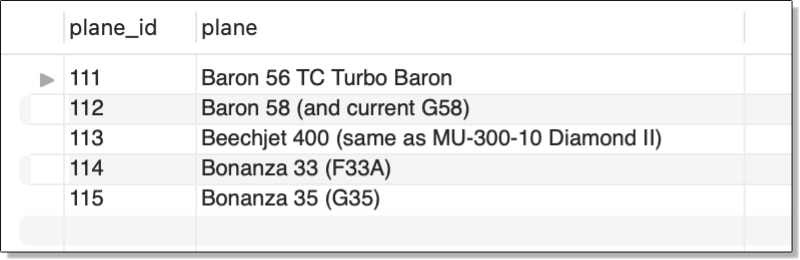
In this case, the subquery is a simple SELECT statement that returns the manufacturer_id value for the manufacturer named Beechcraft. This value, 1003, is then passed into the WHERE clause as part of its search condition. If a row in the airplanes table contains a manufacturer_id value that matches 1003, the row is included in the query results, which are shown in the following figure.

The subquery in this example retrieves data from a second table, in this case, manufacturers. However, a subquery can also retrieve data from the same table, which can be useful if the data must be handled in different ways. For example, the subquery in the following SELECT statement retrieves the average max_weight value from the airplanes table:

SELECT plane_id, plane, max_weight
FROM airplanes
WHERE max_weight > 
  (SELECT AVG(max_weight) FROM airplanes);

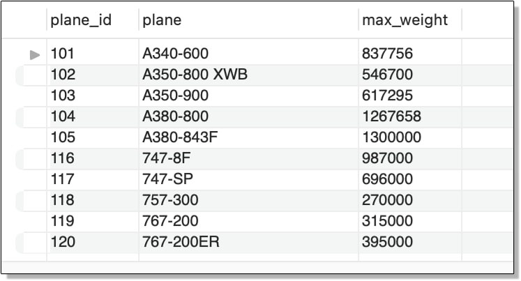
The WHERE clause search condition in the outer statement uses the average to return only rows with a max_weight value greater than that average. If you were to run the subquery on its own, you would see that the average maximum weight is 227,499 pounds. As a result, the outer SELECT statement returns only those rows with a max_weight value that exceeds 227,499 pounds, as shown in the following figure.

As I mentioned earlier in the article, you can use subqueries in statements other than SELECT. One of those statements is the SET statement, which lets you assign variable values. You can use a SET statement to define a value that can then be passed into other statements. For example, the following SET and SELECT statements implement the same logic as the previous example and return the same results:

SET @avg_weight = 
  (SELECT ROUND(AVG(max_weight)) FROM airplanes);
SELECT plane_id, plane, max_weight
FROM airplanes WHERE max_weight > @avg_weight;

The SET statement defines a variable named @avg_weight and uses a subquery to assign a value to that variable. This is the same subquery that is in the previous example. The SELECT statement then uses that variable in its WHERE clause (in place of the original subquery) to return only those rows with a max_weight value greater than 227,499 pounds.

The examples in this section focused on using scalar subqueries in SELECT statements, but be aware that you can also use them in UPDATE and DELETE statements, as well as the SET clause of the UPDATE.

Working with correlated subqueries

One of the most valuable features of a subquery is its ability to reference the outer query from within the subquery. Referred to as a correlated subquery, this type of subquery can return data that is specific to the current row being evaluated by the outer statement. For example, the following SELECT statement uses a correlated subquery to calculate the average weight of the planes for each manufacturer, rather than for all planes:

SELECT m.manufacturer_id, m.manufacturer, 
  a.plane_id, a.plane, a.max_weight
FROM airplanes a INNER JOIN manufacturers m
  ON a.manufacturer_id = m.manufacturer_id
WHERE a.max_weight > 
  (SELECT ROUND(AVG(max_weight)) FROM airplanes a2
    WHERE a.manufacturer_id = a2.manufacturer_id);

Unlike the previous two examples, the subquery now includes a WHERE clause that limits the returned rows to those with a manufacturer_id value that matches the current manufacturer_id value in the outer query. This is accomplished by assigning an alias (a) to the table in the outer query and using that alias when referencing the table’s manufacturer_id column within the subquery.

In this case, I also assigned an alias (a2) to the table referenced within the subquery, but strictly speaking, you do not need to do this. I like to include an alias for consistency and code readability, but certainly take whatever approach works for you.

To better understand how the subquery works logically (as opposed to how the optimizer might actually execute it), consider the first row in the airplanes table, which has a manufacturer_id value of 1001.

When the outer query evaluates the first row, it compares the max_weight value to the value returned by the subquery. To carry out this comparison, the database engine first matches the manufacturer_id value in the outer query to the manufacturer_id values returned by the subquery’s SELECT statement. It then finds all rows associated with the current manufacturer and returns the average max_weight value for that manufacturer, repeating the process for each manufacturer returned by the outer query.

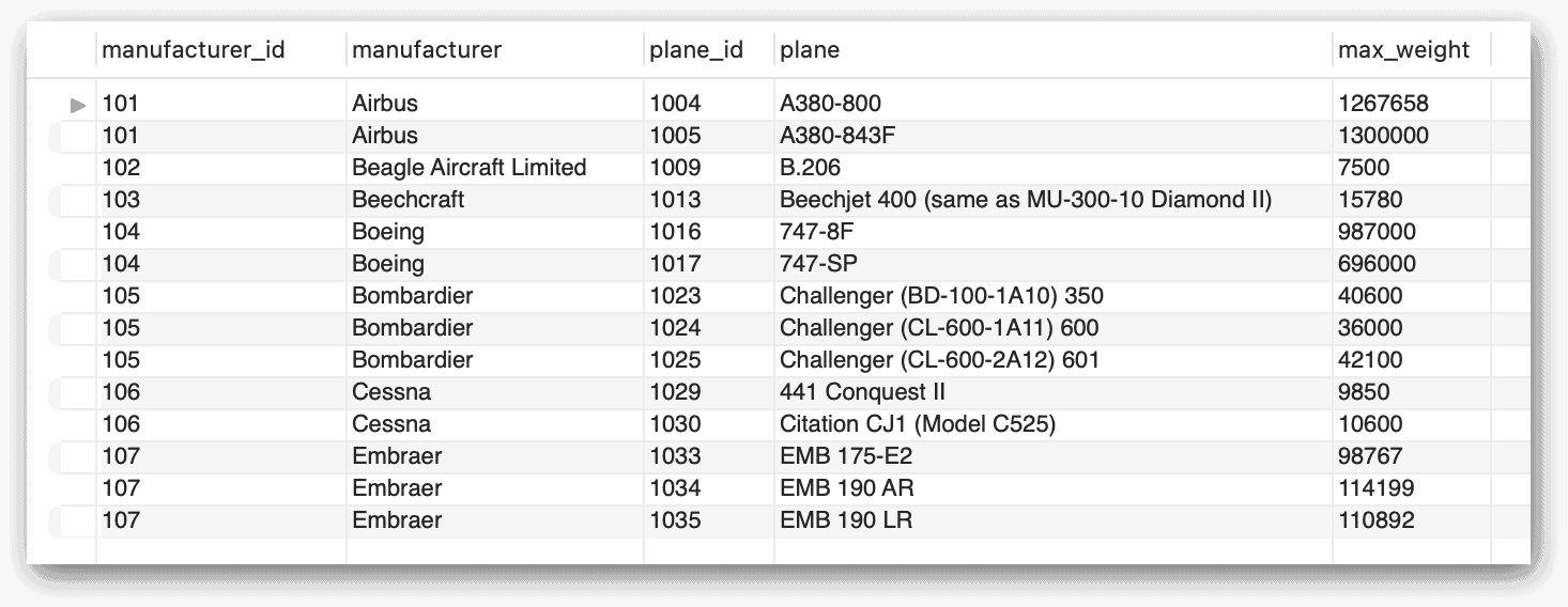
The following figure shows the results returned by the outer SELECT statement. The max_weight values are now compared only with the manufacturer-specific averages.

You can also use this same subquery in the SELECT clause as one of the column expressions. In the following example, I added the subquery after the max_weight column and assigned the alias avg_weight to the new column:

SELECT manufacturer_id, plane_id, plane, max_weight,
  (SELECT ROUND(AVG(max_weight)) FROM airplanes a2
    WHERE a.manufacturer_id = a2.manufacturer_id) AS avg_weight
FROM airplanes a
WHERE max_weight > 
  (SELECT ROUND(AVG(max_weight)) FROM airplanes a2
    WHERE a.manufacturer_id = a2.manufacturer_id);

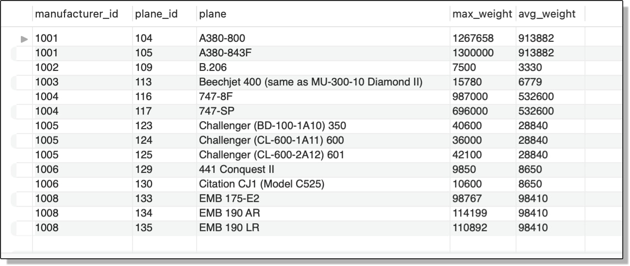
The new subquery works the same as in the preceding example. It returns the average weight only for the planes from the current manufacturer, as shown in the following figure.

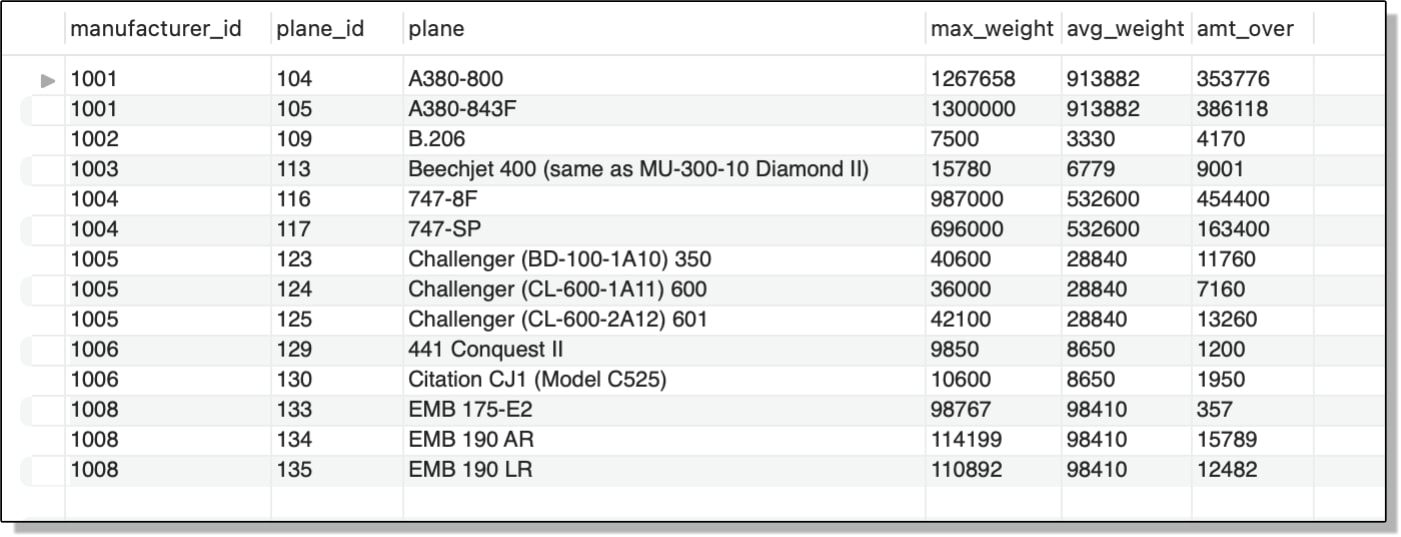
In the previous example, I used a subquery to create a generated column. However, you can use a subquery when creating an even more complex generated column. In the following example, I’ve added a generated column named amt_over, which subtracts the average weight returned by the subquery from the weight in the max_weight column:

SELECT manufacturer_id, plane_id, plane, max_weight,
  (SELECT ROUND(AVG(max_weight)) FROM airplanes a2
    WHERE a.manufacturer_id = a2.manufacturer_id) AS avg_weight,
  -- subtracts average weight from max weight
  (max_weight - (SELECT ROUND(AVG(max_weight)) FROM airplanes a2
    WHERE a.manufacturer_id = a2.manufacturer_id)) AS amt_over
FROM airplanes a
WHERE max_weight > 
  (SELECT ROUND(AVG(max_weight)) FROM airplanes a2
    WHERE a.manufacturer_id = a2.manufacturer_id);

The avg_weight column in the SELECT list is a generated column that uses a subquery to return the average weight of the current manufacturer. The amt_over column is also a generated column and it uses the same subquery to return the average weight. Only this time, the column subtracts that average from the max_weight column to return the amount that exceeds the average.

The following figure shows the results now returned by the outer SELECT statement. As you can see, they include the amt_over generated column, which shows the differences in the weights.

If you want, you can also retrieve the name of the manufacturer from the manufacturers table and include that in your SELECT clause, as shown in the following example:

SELECT manufacturer_id, 
  (SELECT manufacturer FROM manufacturers m 
    WHERE a.manufacturer_id = m.manufacturer_id) manufacturer,
  plane_id, plane, max_weight,
  (SELECT ROUND(AVG(max_weight)) FROM airplanes a2
    WHERE a.manufacturer_id = a2.manufacturer_id) AS avg_weight,
  (max_weight - (SELECT ROUND(AVG(max_weight)) FROM airplanes a2
    WHERE a.manufacturer_id = a2.manufacturer_id)) AS amt_over
FROM airplanes a
WHERE max_weight > 
  (SELECT ROUND(AVG(max_weight)) FROM airplanes a2
    WHERE a.manufacturer_id = a2.manufacturer_id);

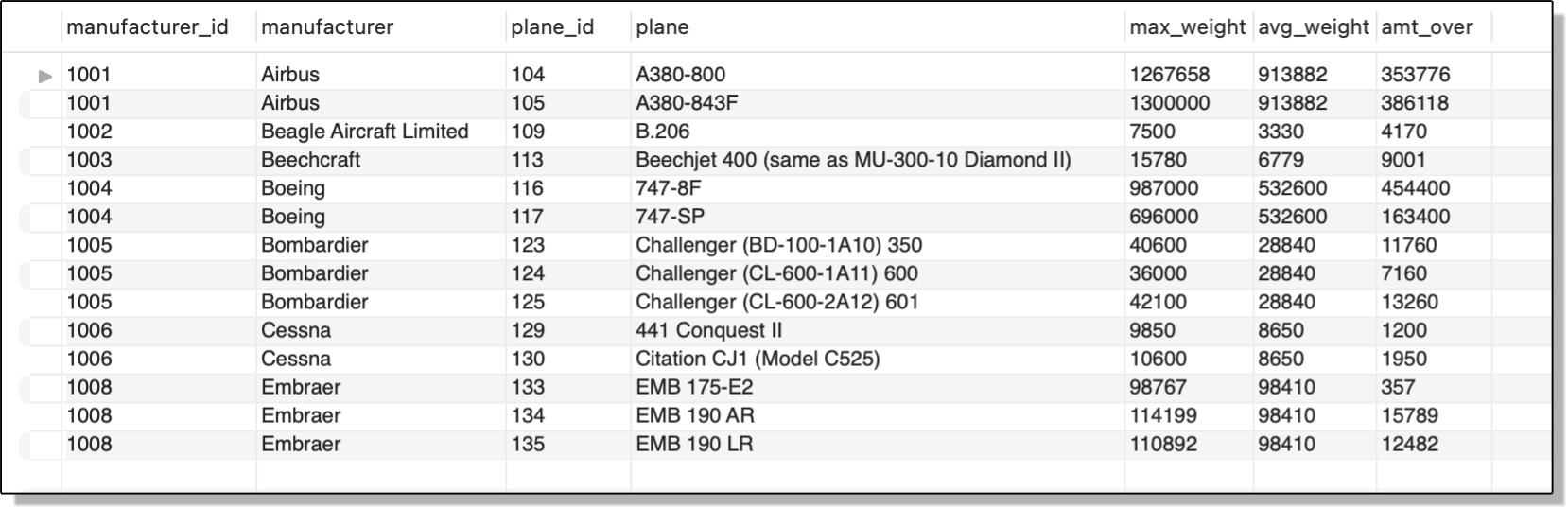
This statement is similar to the previous statement except that it adds the manufacturer column, a generated column. The new column uses a subquery to retrieve the name of the manufacturer from the manufacturers table, based on the manufacturer_id value returned by the outer query.

In some cases, a subquery might not perform as well as other types of constructs. For example, MySQL can often optimize a left outer join better than a subquery that carries out comparable logic. If you’re using a subquery to perform an operation that can be achieved in another way and are concerned about performance, you should consider testing both options under a realistic workload to determine which is the best approach.

The following figure shows the results with the additional column, which I’ve named manufacturer.

One other detail I want to point out about using subqueries in the SELECT list is that you can include them even if you’re grouping and aggregating data. For instance, the following SELECT statement includes a subquery that retrieves the name of the manufacturer associated with each group:

SELECT manufacturer_id, 
  (SELECT manufacturer FROM manufacturers m 
    WHERE a.manufacturer_id = m.manufacturer_id) manufacturer,
  COUNT(*) AS plane_amt
FROM airplanes a
WHERE engine_type = 'piston'
GROUP BY manufacturer_id
ORDER BY plane_amt DESC;

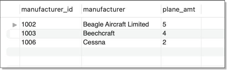
The subquery in this statement is similar to those you’ve seen in other examples, except that now you’re dealing with aggregated data, so the subquery must use a column that is mentioned in the GROUP BY clause of the outer statement, which it does (the manufacturer_id column). The statement returns the results shown in the following figure.

As you can see, the data has been grouped based on the manufacturer_id column, and the name of the manufacturer is included with each ID. In addition, the number of airplanes with piston engines is provided for each manufacturer, with the results sorted in descending order, based on that amount.

Working with a row of data

So far, all the examples in this article have returned scalar values, but your subqueries can also return multiple values, as noted earlier. For example, it might be useful to use a subquery to aggregate a table’s data, calculate specific averages in that data (returned as a single row), and then retrieve rows from the same table that exceed those averages, which is what I’ve done in the following SELECT statement:

SELECT 
  (SELECT manufacturer FROM manufacturers m 
    WHERE a.manufacturer_id = m.manufacturer_id) manufacturer,
        plane_id, plane, max_weight, parking_area,
  (SELECT ROUND(AVG(max_weight)) FROM airplanes a2
    WHERE a.manufacturer_id = a2.manufacturer_id) AS avg_weight,
  (SELECT ROUND(AVG(parking_area)) FROM airplanes a2
    WHERE a.manufacturer_id = a2.manufacturer_id) AS avg_area
FROM airplanes a
WHERE (max_weight, parking_area) > 
  (SELECT ROUND(AVG(max_weight)), ROUND(AVG(parking_area)) 
    FROM airplanes a2
    WHERE a.manufacturer_id = a2.manufacturer_id);

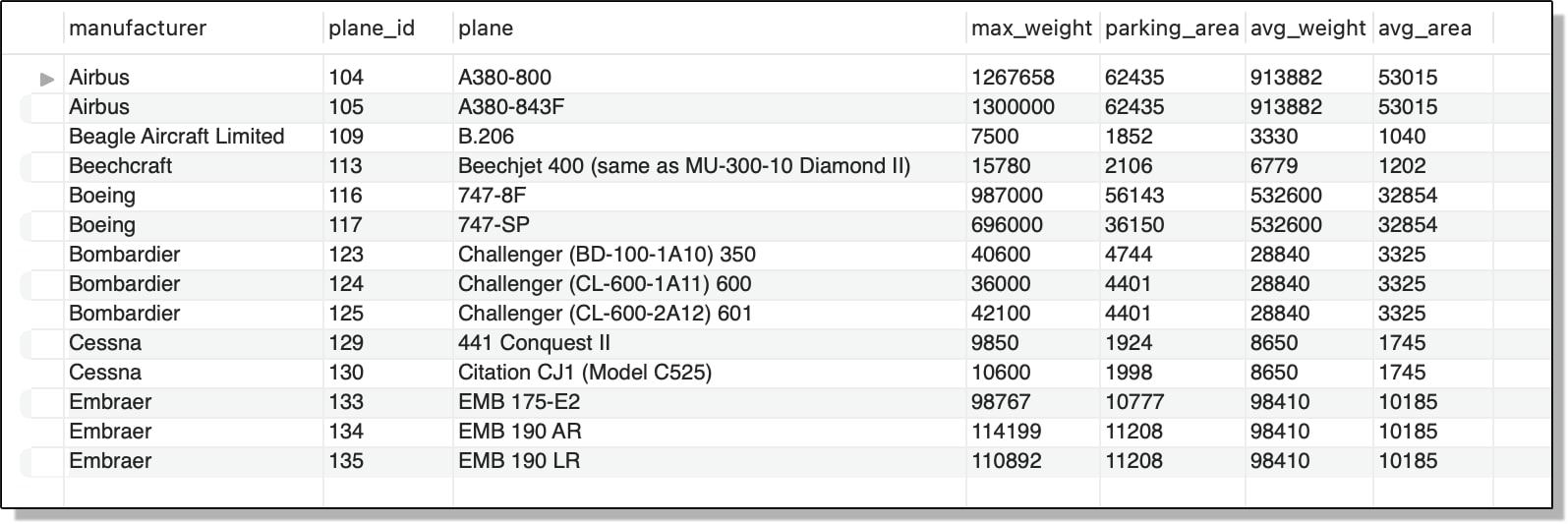
Notice that the WHERE clause in the outer statement includes the max_weight and parking_area columns in parentheses. In MySQL, this is how you create what is called a row constructor, a structure that supports simultaneous comparisons of multiple values. In this case, the row constructor is compared to the results from the subquery, which returns two corresponding values. The first value is the average weight, as you saw earlier. The second value returns the average parking area, which is based on the values in the parking_area column.

In both cases, the averages are specific to the current manufacturer_id value in the outer query. For the outer query to return a row, the two values in the row constructor must be greater than both corresponding values returned by the subquery. Notice also that the SELECT list now includes both the max_weight and parking_area columns, along with the average for each one. The outer statement returns the results shown in the following figure.

One thing you might have noticed about the subqueries in the preceding examples, particularly those used in the WHERE clauses, is that all the search conditions in those clauses use basic comparison operators, either equal (=) or greater than (>). However, you can use any of the other comparison operators, including special operators such as IN and EXISTS, as you’ll see in the next section.

Working with a column of data

The previous section covered row subqueries. A row subquery can return only a single row, although that row can include one or more columns. This is in contrast to a scalar subquery , which returns only a single row and single column. In this section, we’ll look at the column subquery, which returns only a one column with one or more rows.

As with row subqueries, column subqueries are often used in the WHERE clause when building your search conditions. Also like row subqueries, your search condition must take into account that the subquery is returning more than one value.

For example, the WHERE clause in the following SELECT statement uses the IN operator to compare current the manufacturer_id value in the outer statement with the list of manufacturer_id values returned by the subquery:

SELECT manufacturer_id, manufacturer 
FROM manufacturers
WHERE manufacturer_id IN 
  (SELECT DISTINCT manufacturer_id FROM airplanes
    WHERE engine_type = 'piston');

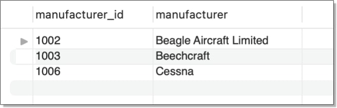
The column data returned by the subquery includes only those manufacturers that offer planes with piston engines (as reflected in the current data set). The IN operator determines whether the current manufacturer_id value is included in that list. If it is, that row is returned, as shown in the following figure.

As with many operations in MySQL, you can take different approaches to achieve the same results. For example, you can replace the IN operator with an equal comparison operator, followed by the ANY keyword, as shown in the following example:

SELECT manufacturer_id, manufacturer 
FROM manufacturers
WHERE manufacturer_id = ANY 
  (SELECT DISTINCT manufacturer_id FROM airplanes
    WHERE engine_type = 'piston');

You could have instead used another comparison operator, such as greater than (>) or lesser than (<) or even ALL instead of ANY. The statement returns the same results as the previous example. In fact, you can also achieve the same results by rewriting the entire statement as an inner join:

SELECT DISTINCT m.manufacturer_id, m.manufacturer
FROM manufacturers m INNER JOIN airplanes a
  ON m.manufacturer_id = a.manufacturer_id
WHERE a.engine_type = 'piston';

I’m not going to go into joins here, but as I mentioned earlier, joins can sometimes provide performance benefits over subqueries, so you should be familiar with how they work and how they differ from subqueries (a topic that could easily warrant its own article).

With that in mind, be aware that you can also use the NOT keyword with some operators to return different results. For example, the WHERE clause in the following SELECT statement uses the NOT IN operator ensure the current manufacturer_id value is not in the list of values returned by the subquery:

SELECT manufacturer_id, manufacturer 
FROM manufacturers
WHERE manufacturer_id NOT IN 
  (SELECT DISTINCT manufacturer_id FROM airplanes);

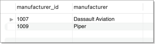
In this case, the subquery returns a distinct list of all manufacturer_id values in the airplanes table. The list is then compared to each manufacturer_id value in the manufacturers table, as specified by the outer query. If the value is not in the list, the search condition evaluates to true and the row is returned. In this way, you can determine which manufacturers are in the manufacturers table but are not in the airplanes table. The query results are shown in the following figure.

Be very careful when using NOT IN with your subqueries. If the subquery returns a NULL value, your WHERE expression will never evaluate to true.

Another operator you can use in the WHERE clause is EXISTS (and its counterpart NOT EXISTS). The EXISTS operator simply checks whether the subquery returns any rows. If it does, the search condition evaluates to true, otherwise it evaluates to false. For example, the following SELECT statement defines similar logic as the preceding example, except that it checks for which manufacturers are included in both tables:

SELECT manufacturer_id, manufacturer 
FROM manufacturers m
WHERE EXISTS
  (SELECT * FROM airplanes A
    WHERE a.manufacturer_id = m.manufacturer_id);

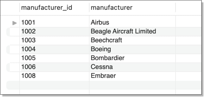
Notice that you need only specify the EXISTS operator followed by the subquery. If the subquery returns a row for the current manufacturer_id value, the search condition evaluates true and the outer query returns a row for that manufacturer. The following figure shows the results returned by the statement.

When working with column subqueries, it’s important to understand how to use comparison operators such as IN, NOT IN, ANY, ALL, and EXISTS. If you’re not familiar with them, be sure to refer to the MySQL documentation to learn more.

Using subqueries in the FROM clause

In addition to rows, columns, and scalar values, subqueries can also return tables, which are referred to as derived tables. Like other subqueries, a table subquery must be enclosed in parentheses. In addition, it must also be assigned an alias, similar to specifying a table alias when building correlated subqueries. For example, the following SELECT statement includes a table subquery named total_planes, which is included in the FROM clause of the outer statement:

SELECT ROUND(AVG(amount), 2) avg_amt
FROM 
  (SELECT manufacturer_id, COUNT(*) AS amount 
  FROM airplanes
  GROUP BY manufacturer_id) AS total_planes;

Notice that the outer statement does not specify a table other than the derived table returned by the subquery. The subquery itself groups the data in the airplanes table by the manufacturer_id values and then returns the ID and total number of planes in each group. The outer statement then finds the average number of planes across all groups. In this case, the statement returns a value of 5.00.

Now let’s look at another example of a table subquery. Although this next example is similar to the previous one in several ways, it includes something you have not seen yet, one subquery nested within another. In this case, I’ve nested a table subquery within another table subquery to group data based on custom categories and then find the average across those groups:

-- outer SELECT calculates average count across all categories
SELECT
  ROUND(AVG(amount), 2) AS avg_amt
FROM
  -- outer subquery aggregates categories and calculates count for each one
  (SELECT category, COUNT(*) amount 
  FROM 
    -- inner subquery categorizes planes based on parking area
    (SELECT CASE
      WHEN parking_area > 50000 THEN 'A'
      WHEN parking_area >= 20000 THEN 'B'
      WHEN parking_area >= 10000 THEN 'C'
      WHEN parking_area >= 5000 THEN 'D'
      WHEN parking_area >= 1000 THEN 'E'
      ELSE 'F'
    END AS category
    FROM airplanes) AS plane_size
  GROUP BY category
  ORDER BY category) AS plane_cnt;

The innermost subquery—the one with the CASE expression—assigns one of five category values (A, B, C, D, E, and F) to each range of parking area values. The subquery returns a derived table named plane_size, which contains a single column named category. The column contains a category value for each plane in the airplanes table.

The data from the plane_size table is then passed to the outer subquery. This subquery groups the plane_size data based on the category values and generates a second column named amount, which provides the total number of planes in each category. The outer subquery returns a derived table named plane_cnt. The outer statement then finds the average number of planes across all groups in the derived table, returning a value of 5.83.

Working with MySQL subqueries

Like many aspects of MySQL, the topic of subqueries is a much broader than what can be covered in a single article. To help you complete the picture, I recommend that you also check out the MySQL documentation on subqueries, which covers all aspects of how to use subqueries. In the meantime, you should have learned enough here to get a sense of how subqueries work and some of the ways you can use them in your SQL statements. Once you have a good foundation, you can start building more complex subqueries and use them in statements other than SELECT queries. Just be sure to keep performance in mind and consider alternative statement strategies, when necessary, especially if working with larger data sets.


The post Subqueries in MySQL appeared first on Simple Talk.


from Simple Talk https://ift.tt/PRWcA0Q
via

Thursday, December 1, 2022

Backing Up MySQL Part 6: Physical vs. Logical Backups

Everyone who has ever backed up data using any kind of RDBMS knows a thing or two about backups. Backups are a central part of data integrity – especially nowadays, when data breaches are happening left and right. Properly tested backups are crucial to any company: once something happens to our data, they help us quickly get back on track. However, some of you may have heard about the differences between backups in database management systems – backups are also classified into a couple of forms unique to themselves. We’re talking about the physical and logical forms – these have their own advantages and downsides: let’s explore those and the differences between the two. This tutorial is geared towards MySQL, but we will also provide some advice that is not exclusive to MySQL.

What are Logical Backups?

Logical backups are backups of data consisting of statements that let the database recreate the data. Think of how you usually take backups within MySQL – no matter if you find yourself using the Export functionality within phpMyAdmin or using mysqldump to back up your most precious data, both of those measures have the same thing in common – they create statements that recreate data, creating logical backups as a result. And that’s exactly what defines logical backups – logical backups aim to recreate data by running SQL statements.

Sometimes though, developers might find themselves in waters where recreation of files is required.

What are Physical Backups?

Physical backups, as you might’ve guessed, copy the “physical” data – files – that comprise a database. As far as MySQL is concerned, the physical backup of MySQL usually consists of a copy of the data directory found here (Windows-based example – in Linux, the directory would be /var/lib/mysql/mysql5.7.36/data):

Logical Backups in MySQL

Taking logical backups within MySQL is easier than you might’ve guessed – think of any part of MySQL that backs up statements to recreate data. Got one? You’ve got yourself a logical backup!

In MySQL, logical backups are taken by:

  • The Export functionality in phpMyAdmin
  • Using mysqldump
  • Or using the SELECT [columns] INTO OUTFILE [path] statement in a specific database:

phpMyAdmin

Contrary to popular belief, the export functionality within phpMyAdmin can offer quite a lot of options to choose from. Users have a variety of options to choose from, including, but not limited to:

  • The ability to choose whether to back up table structure, data, or both;
  • The ability to choose the format of the backup;
  • The option to can lock the tables while data is being written to them;
  • The ability to export tables as separate files;
  • The ability to compress the backup, skip tables larger than a specified value, etc.

Some of the abilities of phpMyAdmin can be seen below:

Since phpMyAdmin is one of the most widely used tools within MySQL, it’s logical (see what we did there?) that it offers a lot of options for both junior developers and experienced DBAs alike (see example above.) phpMyAdmin isn’t anything fancy and it’s been here for decades – yet, its slick UI and rich feature set make it stand out from the crowd.

mysqldump

The next tool in the toolset of a MySQL DBA is, of course, mysqldump itself – the tool works much like the Export functionality within MySQL, just that it’s command line-based. For all of the nitty-gritty details, refer to the first blog of these series, but in a nutshell, mysqldump is once again blessed with an extremely rich set of features including, but not limited to:

  • An ability to let backups continue being performed even if errors are encountered.
  • An ability to only dump the schema within the tables.
  • Only dump data matching a specific WHERE clause.

In order to use mysqldump, we need to be privileged enough to issue SELECT queries, and the syntax would look something similar to the following statement (to be issued before you log in to your database via the CLI on Windows or Linux):

If you’re security minded, keep in mind that you can also prevent yourself from providing a username (-u) and the password (-p) by specifying it in the main configuration file of MySQL under the [mysqldump] heading like so (specify the user and password variables) – doing so will prevent anyone from seeing your username and password in the list of last issued commands in Linux:

For many people, phpMyAdmin and mysqldump provides enough of a grip into the world of backups – however, some might say the capabilities of the tools are a little lacking; those who venture into the world of big data might have to confirm the statement from experience – while both phpMyAdmin and mysqldump can offer powerful methods to back your data up in a fashion that is quicker than usual (LOCK TABLES provides developers with the ability to lock tables for a certain time until the backup is finished making its operations significantly quicker), both of those methods have a glaring flaw – the backups they create are riddled with INSERT statements.

There’s nothing “wrong” with INSERT statements per se, but their weakness is that they’re very ill-equipped to handle anything more than a couple million rows at a time: the core reason behind this is that INSERT statements come with a lot of overhead that MySQL has to consider – amongst other things, that includes parsing too. Imagine running 500,000 INSERT queries one after another where MySQL has to complete the following steps:

  1. Start.
  2. Check for permissions.
  3. Open tables.
  4. Initialize the query.
  5. Acquire locks.
  6. Do its work (run the query.)
  7. Finish (“end”) the query.
  8. Close tables.
  9. Clean up.

Complete these steps. Now complete them again and repeat everything for additional 499,998 iterations. Does that sound quick? Sure, if we lock the tables, we might avoid the steps #3 and #8, but our queries will be slow nonetheless – there are a lot of things MySQL has to consider when running INSERT queries. There is a solution, though – we should also look into the LOAD DATA INFILE [path] INTO TABLE [table] query which is specifically designed for big data sets.

SELECT INTO OUTFILE & LOAD DATA INFILE

An alternative to INSERT that’s specifically designed for big data sets looks something like this:

LOAD DATA INFILE ‘/tmp/data.txt’ INTO TABLE demo_table [FIELDS TERMINATED BY|OPTIONALLY ENCLOSED BY] “|”;

That’s the LOAD DATA INFILE query, of course. It’s designed specifically for bulk data loading, and it’s capable of loading data in with “bells and whistles”:

  • It’s able to skip certain lines or columns.
  • It’s able to only load data into specific columns.
  • It comes with significantly less overhead for parsing.

When LOAD DATA INFILE is in use, MySQL doesn’t perform as many operations as it does when INSERT INTO is in use, making operations significantly faster. To take a backup of your big data set use its brother – SELECT * INTO OUTFILE – like so:

Then use LOAD DATA INFILE to load data back into your database (here we also use the IGNORE statement to ignore all potential errors – duplicate key issues, etc.):

Recap

  • Backups taken by both phpMyAdmin and mysqldump can be simply re-imported into MySQL by using a simple query like so or via the phpMyAdmin interface (remove the -u and -p options if the username and password is specified in my.cnf):
    mysql -u root -p [database_name] < database_backup.sql
  • To restore a backup taken using SELECT … INTO OUTFILE, use LOAD DATA INFILE.

However, while these three options comprise logical backups – the most frequently used form of backups in MySQL – and the process of taking them is quick, easy and straightforward, keep in mind that there’s also another way to accomplish your goals – people can also take backups in a physical form. Such backups copy files containing the data instead of recreating statements that build the data.

Physical Backups in MySQL

Physical backups offer the ability to copy files (physical data) instead of the statements that recreate it. To take a physical backup in MySQL:

  1. Make sure MySQL is shut down (otherwise we’d be copying files that MySQL is still working with.)
  2. Head over to the data directory (entering SELECT @@datadir while logged in to your MySQL instance will help you see where it is):

  1. Head over to the directory where you’ll store the physical backup, then create a directory inside of it using mkdir:
    mkdir [directory_name]
  2. Copy the files named ibdata1 (the main tablespace file of InnoDB), ib_logfile0 and ib_logfile1 (undo and redo logs exclusive to InnoDB) to the directory you just created, then copy the data directory itself. Do note that if the data directory is big, copying operations will take some time.
  3. You just took a physical backup!

If, for some reason, you find yourself using MyISAM (which is obsolete at the time of writing), taking physical backups of it is even easier – you just need to copy the data folder containing your databases, their data (.MYD files) and associated indexes (.MYI files.)

Physical backups can be useful when there’s a necessity to restore everything from a database from some media storage in one go, however, some might call the process of taking them a little tedious. To each their own though.

Recap

Physical backups copy the files that the data is based upon – to take a copy of them when using InnoDB, take a copy of the InnoDB tablespace (ibdata1) and the undo & redo logs (ib_logfile0 & ib_logfile1), then the data folder. To back up MyISAM, take a copy of all of the data and index files (.MYD and .MYI files) in the data folder.

Summary

MySQL offers everyone a couple of ways to back up data – while the most common option are logical backups that back up statements that recreate the data, indexes, partitions, and all related details, some might make use of physical backups where users copy the data files themselves: each option has its own upsides and downsides, so make sure to try both options out before your plan out your backup strategy. Familiarize yourself with all of the options, then make your own, physical or logical, decision.

We hope that this blog has been informational and that you’ve learned something new, and until next time!

The post Backing Up MySQL Part 6: Physical vs. Logical Backups appeared first on Simple Talk.


from Simple Talk https://ift.tt/TMdH0CE
via