Monday, February 28, 2022

Azure: Small Changes that Matter

I believe I’m not alone on this feeling: It seems like every time we use the Azure Portal some new feature appear. The features reproduce themselves faster than rabbits. Did you had this feeling before? Share your thoughts in the comments.

This week, working with Azure, I found some new small features around and decided to share them with you. When does these features appeared? Where did they come from? No idea, but they are interesting. It’s even possible they were there for some time and I never reached them. Anyway, Tighten your seat belt and prepare for a ride.

Deletion features on virtual machines

When we provision a virtual machine, many additional objects are provisioned together it: Disk (or disks), Network Interface and Public IP, for example.

This usually creates problems when deleting a VM. If you have multiple VMs in the same resource group, you need to locate each object related to the VM and delete them.

Some features, such as Availability Sets and Site Recovery, requires us to provision multiple VMs in the same resource group. This requirement and the deletion problem annoys me a lot. Provisioning on this way creates problems when deleting the VM. It becomes difficult to select the correct objects. Sometimes Azure also has problems identifying the correct deletion order, according the objects dependencies.

The new feature: We have two deletion checkboxes included during the provision of a virtual machine. The first one, to delete the disks together the virtual machine itself, the other to delete the network interface together the virtual machine itself.


The deletion process, by the way, deserves a special mention: I spent an entire week working with Azure without getting a single deletion error – when azure mistakes the order to delete dependent objects. This is great!

Global load balancer

The Load Balancer, a layer 3 load balancer in Azure, got a new option for us to select: Regional or Global.

Regional load balancer is the load balancer we are familiar with, no difference. Global load balancer is a load balancer which only accepts other load balancers on the backend pool. Yes: A load balancer of load balancers.

It can load balance across different regions. This means we can create two set of VMs, each one on a different region and using a regional load balancer for them, then create a Global Load balancer to balance the load between them.

This feature can twist the reality but doesn’t change it: There are two local load balancers in Azure and two Global load balancers in Azure. Load Balancer and Application Gateway are local load balancers while Traffic Manager and Front Door are global load balancers.

A local load balancer requires the connection from the end user to reach it, on the region it’s deployed. A global load balancer, on the other end, intercepts the request anywhere in the world, on the border of the Azure network, and process the request, without being tied with a region.

One side note about this change is the mix of names: Now, “Global” for load balancers have two different meanings depending on the context.

Internal Load Balancer

The type selection for Public or Internal load balancer also seems new. The load balancer was public by default. The new internal load balancer option changes the front-end IP configuration and only allow us to set an internal IP as the front-end IP.

An internal Load Balancer can be used by internal applications, put behind another load balancer or exposed to the internet using NAT.

Gateway Load Balancer

This is a new SKU for the load balancer. This feature is in preview, but I could only notice this when checking the documentation.


A Gateway load balancer works as a load balancer/gateway for NVA’s. It redirects traffic to NVA’s, allowing them to work as firewalls, analyse the network traffic and many additional tasks.


Public load balancers have the option to redirect their traffic to the NVA’s, using the Gateway Load Balancer. According to the documentation, we also should be able to configure network interfaces to redirect their traffic to the gateway load balancer. However, I couldn’t find this option on network interfaces in the portal. Maybe it’s because it’s still in preview.


The possibility to configure the gateway load balancer in network interfaces avoid the need of custom routing tables for a NVA. I would still question what would be best: using a custom routing table set on the subnet or configuring each network interface.

New advanced backup option

This is a very interesting and simple improvement. When configuring backup for a VM to recovery services vault, we were limited to once a day backup. Anything beyond that required a custom backup server.

I don’t know exactly why this option appear like it was a total different kind of backup. It seems to me the improvement from once a day to hourly backup is the main new feature here.


There is an additional difference: The amount of backups to be retained on the source machine. Originally it was 5, while with the new backup it’s up to 30. It makes sense: if you are making a daily backup, you don’t need to retain many of them. On the other hand, if you are making hourly backups, you may need to retain 1 day or more.

The images below show the difference between the retention on the old and new backup method.


The hourly backup feature, however, is only available under request to join the preview. On the other hand, the change on the retention days is available.

Choice of what will be encrypted in a storage account

The possibility to encrypt a storage account using a customer managed key is very interesting. It’s not a new feature at all.

The new feature is the possibility to select the services affected by the customer managed key: Blob Storage, File Storage, Tables or Queues.


It escapes to me why someone would like to apply the encryption key to only some services.

Link to set the permissions for a VPN Gateway

This is, probably, the most hidden of the new features. When we configure a point to site VPN to use Azure Authentication, we need to give permission to Azure VPN App to access our Azure Active Directory.

This requires us to follow a detailed documentation from Microsoft website to build a complex URL and call it on the browser.

The new feature: Now we have a link on the configuration page. Clicking on the link we trigger the same URL, setting the permission to Azure VPN.


One complex URL less to build while configure Azure Authentication for a VPN. A few helpers more on the text boxes and we will not need to open the documentation anymore to complete this configuration.

DSC on a Virtual Machine

The Desired State Configuration made from a Virtual Machine blade instead of an Automation Account is already in preview for some time. The first time I tested it, the results were not much integrated with the automation account.

The news is that now the synchronization between automation account and the DSC on the VM is way better. After applying the DSC on the automation account, I was able to see the same configuration on the DSC blade of the virtual machine.


The button Manage Multiple Machines on a single virtual machine takes us to the automation account used to complete the DSC configuration. The synchronization is way better.

References

Gateway Load Balancer

https://docs.microsoft.com/en-us/azure/load-balancer/gateway-overview 

Configure Azure Authentication on a VPN Gateway

https://docs.microsoft.com/en-us/azure/vpn-gateway/openvpn-azure-ad-tenant   

Create an Internal Load Balancer

https://docs.microsoft.com/en-us/azure/load-balancer/quickstart-load-balancer-standard-internal-portal?tabs=option-1-create-internal-load-balancer-standard

The post Azure: Small Changes that Matter appeared first on Simple Talk.


from Simple Talk https://ift.tt/Xs29rkB
via

Working with MySQL tables

The series so far:

  1. Getting started with MySQL
  2. Working with MySQL tables

Tables lie at the heart of any MySQL database, providing a structure for how data is organized and accessed by other applications. Tables also help to ensure the integrity of that data. The better you understand how to create and modify tables, the easier it will be to manage other database objects and the more effectively you can work with MySQL as a whole. Having a solid foundation in tables can also help you build more effective queries so that you’re retrieving the data you need (and only that data), without compromising database performance.

This article is the second in a series on MySQL. I recommend that you review the first article before launching into this one, if you haven’t done so already. In this article, I focus primarily on how to create, alter, and drop tables, demonstrating how to use both SQL statements and the GUI features in MySQL Workbench. As with the first article, I used the MySQL Community edition on a Windows computer to create the examples for this article. All the examples were created in Workbench, which comes with the Community edition.

Using the MySQL Workbench GUI to create a database

Before creating any tables, you need a database for those tables, so I’ll spend a little time on databases first. Creating a database in MySQL is a relatively straightforward process. As you saw in the first article in this series, you can run a simple CREATE DATABASE statement against the target MySQL instance where you want to add the database. This is especially easy if you plan to use the default collation and character set. For example, to create the travel database, you need only run the following statement:

CREATE DATABASE travel;

The CREATE DATABASE statement does exactly what it says. It creates a database on the MySQL instance that you’re connected to. If you want to make sure the database doesn’t exist before running the statement, you can add the IF NOT EXISTS clause:

CREATE DATABASE IF NOT EXISTS travel;

Both statements instruct MySQL to create a database that uses the default collation and character set. You can run either statement from the MySQL command prompt or from within MySQL Workbench. To run a statement in Workbench, you need only open a query tab, type, or paste the statement onto the tab, and click one of the execute buttons on the toolbar. MySQL does the rest.

Instead of using a CREATE DATABASE statement to create a database, you can use a CREATE SCHEMA statement. They both support the same syntax, and both achieve the same results. This is because MySQL treats databases and schemas as one in the same. In fact, MySQL considers CREATE SCHEMA to be a synonym for CREATE DATABASE. When you create a database, you create a schema. When you create a schema, you create a database. Workbench uses both terms, freely switching between one and the other.

You can also use the GUI features built into Workbench to create a database. Although this might seem overkill, given how easy it is to run a CREATE DATABASE statement, the GUI offers the advantage of listing all the character sets and collations available to a database definition, should you decide not to use the defaults.

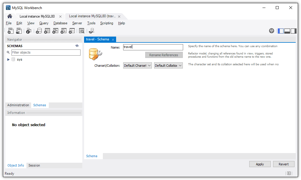
To use the GUI to create a database, start by clicking the create schema button on the Workbench toolbar. (The button looks like a standard database icon and displays the tooltip Create a new schema in the connected server.) When the Schema tab opens, you need only provide a database name, as shown in Figure 1.

An image showing the MySQL Workbench dialog to create a schema/database

Figure 1. Adding a database to a MySQL instance

If you want to use a character set or collation other than the defaults, you can select them from the drop-down lists. For example, you might select utf8 for the character set and utf8_unicode_ci for the collation.

With MySQL, you can set the character set and collation at multiple levels: server, database, table, column, or string literal. The default server character set is utf8mb4, and the default collation is utf8mb4_0900_ai_ci. Before deviating from the defaults, I suggest that you first review the MySQL documentation on character sets and collations.

The Schema tab also includes the Rename References option. However, this is disabled and applies only when you’re updating a database model. Workbench sometimes includes interface options that don’t apply to the current circumstances, which can be confusing when you’re first getting started with MySQL or Workbench. However, you’re usually safe to stick with the default values if you’re not sure about an option, at least until you better understand how it works and whether it’s even applicable.

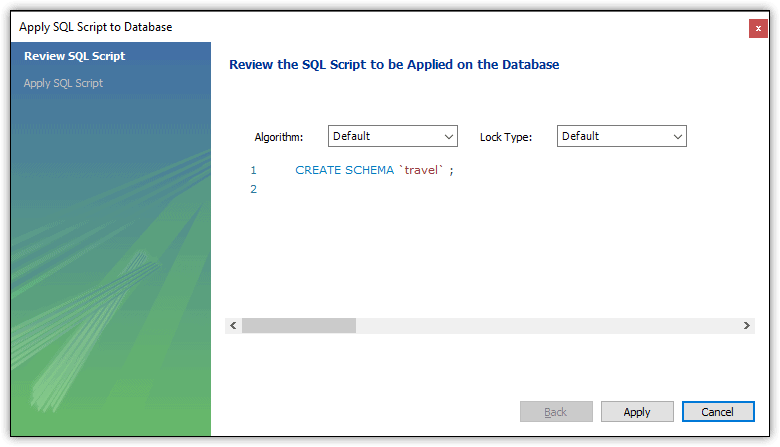
For this article (assuming that you want to follow along with the examples), you can stick with the default character set and collation and click Apply. This will launch the Apply SQL Script to Database wizard, shown in Figure 2. The wizard’s first screen displays the SQL statement that Workbench generated but not yet applied against the MySQL instance.

An image showing the script before it is applied to the database "CREATE SCHEMA 'travel';"

Figure 2. Verifying the CREATE SCHEMA statement

The screen also includes the Algorithm option and Lock Type option. Both options are related to MySQL’s online DDL feature, which provides support for in-place table alterations and concurrent DML. You do not need to be concerned about these options right now and can stick with the defaults. (This is another example of Workbench’s sometimes confusing options.) However, if you’re interested in learning more about these features, you can find information in the MySQL documentation that covers InnoDB and online DDL.

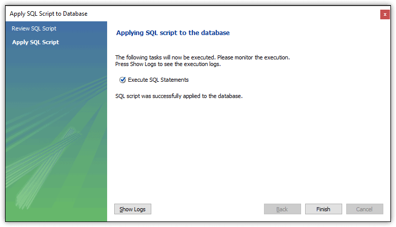
To create the database, click Apply, which takes you to the next screen, shown in figure 3. This screen essentially confirms that the database has been created. You can then click Finish to close the dialog box. Be sure to close the original Schema tab as well.

An image showing the final dialog to apply the script. Click Finish.

Figure 3. Finalizing the new schema (database)

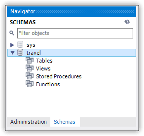
The database should now be listed in the Schemas panel in Navigator. If it is not, click the refresh button in the panel’s upper right corner. The travel database (schema) should then show up along with other databases on the MySQL instance. On my system, the only other database is the default sys database, as shown in Figure 4.

An image showing the new database (schema) in the navigator

Figure 4. Viewing the new database in Navigator

At this point, MySQL has created only the database structure. You can now add tables to the database, along with views, stored procedures, and functions.

Using the MySQL Workbench GUI to create a table

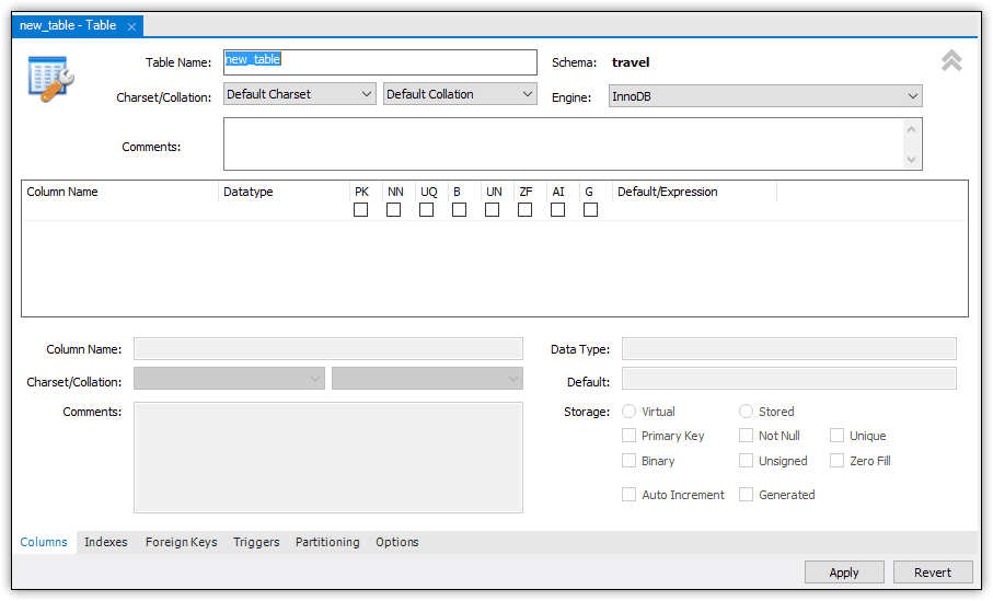
You can also use the Workbench GUI to add a table a database. For this approach, start by selecting the travel database node in Navigator. You might need to double-click the node to select it. The database name should be bold once selected. With the database selected, click the create table button on the Workbench toolbar. (The button looks like a standard table icon and includes the tooltip Create a new table in the active schema in connected server.) When you click the button, Workbench opens the Table tab, as shown in Figure 5.

The New Table GUI. Add columns with datatype and constraints

Figure 5. Adding a table through the Workbench GUI

The tab provides a detailed form for adding columns to the table and configuring table and column options. The tab also includes several of its own tabs (near the bottom of the interface). The Columns tab is selected by default, which is where you’ll be doing most of your work.

Start by providing a name for the table. For this article, I used manufacturers. I also stuck with the default character set and collation, as well as the default storage engine, InnoDB. The InnoDB engine is considered a good general-purpose storage engine that balances high reliability and high performance.

MySQL also supports other storage engines, such as MyISAM, MEMORY, CSV, and ARCHIVE. Each one has specific characteristics and uses. For now, I recommend that you stick with the default InnoDB until you better understand the differences between storage engines. I also recommend that you review the MySQL documentation for detailed information about the different engine types.

At this point, you can also add a table-level comment if you’re so inclined. Although that’s not necessary for this article, information of this sort can be useful when building a database for production.

Once you have the basics in place, you can add the first column, which will be named manufacturer_id. It will also be the primary key and include the AUTO_INCREMENT option, which tells MySQL to automatically generate a unique number for that column’s value, similar to the IDENTITY property in SQL Server.

To add the column, double-click the first cell in the grid’s Column Name column and type manufacturer_id. In the Datatype column for that row, type INT or select INT from the drop-down list. Next, select the following check boxes:

  • PK. Configures the column as the primary key.
  • NN. Configures the column as NOT NULL.
  • UN. Configures the INT database as UNSIGNED.
  • AI. Configures the column with the AUTO_INCREMENT option.

With regard to the UNSIGNED option, MySQL lets you specify whether an integer data type is signed or unsigned. If signed, a column’s values can include negative numbers. If unsigned, the values cannot include negative numbers. Integer data types are signed by default. Older MySQL versions permitted you to configure the DECIMAL, DOUBLE, and FLOAT data types as unsigned, but that feature has been deprecated.

Integer signing affects the range of supported values. Consider the INT data type. If a column is defined with a signed INT data type, the column’s values must be between -2147483648 and 2147483647. However, if the data type is unsigned, the values must be between 0 and 4294967295. If you know that a column will never need to store a negative integer, you can define the data type as unsigned to support a greater range of positive integers.

As you configure a column, Workbench updates the option settings in the section below the grid. This bottom section reflects the settings of the column selected in the grid and can be handy when defining multiple columns. The bottom section also provides several additional optional. For example, you can add a comment specific to the selected column. You can also set the character set and collation at the column level (for character data types).

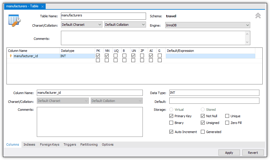
Figure 6 shows the manufacturer_id column as it’s been defined so far. Notice that the bottom section reflects all the settings specified in the column grid.

An image showing the manufacturer_id column with PK (primary key), NN (not null), UN (unsigned), and AI (auto increment) checked. Data type is INT

Figure 6. Adding a column to a table definition

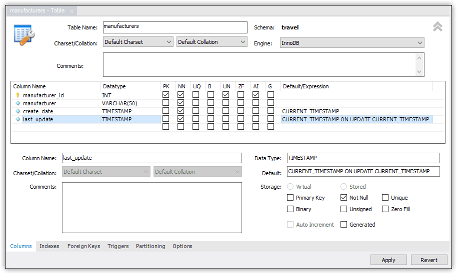
You can repeat a similar process for each additional column you want to include, choosing the data type and configurable options. When specifying the data type, you can type it or select it from the drop-down list. However, some of the data types in the drop-down-list, including TIMESTAMP, are listed with trailing parentheses that should not be there. This is apparently a Workbench bug. You’ll have to manually remove the parentheses for the data type to be listed correctly. You can also specify a default value for any columns you’re defining. For this article, I added three more columns:

  • The manufacturer column is configured with the VARCHAR(50) data type and is NOT NULL.
  • The create_date column is configured with the TIMESTAMP data type and is NOT NULL. It is also configured with the default value CURRENT_TIMESTAMP, a system function that returns the current date and time.
  • The last_update column is configured with the TIMESTAMP data type and is NOT NULL. It is also configured with a default value that include the CURRENT_TIMESTAMP function, along with the ON UPDATE CURRENT_TIMESTAMP option, which generates a value whenever the table is updated.

Figure 7 shows the Table tab after I added the three columns. The grid includes a row for each column, with each row reflecting the column’s configuration.

An image showing the new table dialog with all the columns filled in

Figure 7. Adding multiple columns to the new table definition

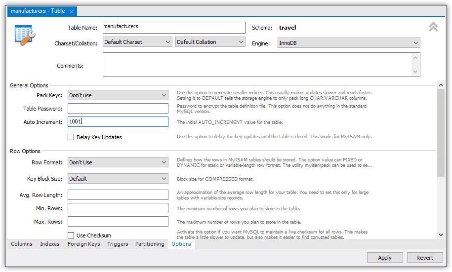
There’s one other step to take to complete the table’s definition. For this, you need to go to the Options tab and set the initial AUTO_INCREMENT seed value. In this case, I used 1001, as shown in Figure 8. As a result, the first record added to the table will be assigned a manufacturer_id value of 1001, with each subsequent row incremented by 1.

An image showing the Auto-increment options. The initial auto-increment value is 1001

Figure 8. Setting the seed value for the AUTO_INCREMENT option

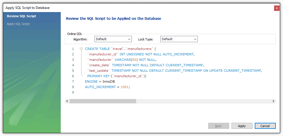
As you can see, there are plenty of other table options that you can configure, and there are other tabs on which you can configure additional options. But for now, we’ll stop here and add the table to the database. To do so, click the Apply button, which launches the Apply SQL Script to Database wizard, shown in Figure 9.

The generated script for the manufacturers table.

Figure 9. Verifying the CREATE TABLE statement

On this screen, you can review the SQL statement that has been generated and select an algorithm and lock type, if desired. You can also edit the SQL statement directly on this screen. (Just be sure not to introduce any errors.)

Notice that the manufacturer_id column is configured with the INT data type (unsigned) and defined as the primary key. It also includes the AUTO_INCREMENT option. The AUTO_INCREMENT seed value, 1001, is specified as a table option, along with the InnoDB storage engine. Notice, too, that the create_date and last_update columns include the specified DEFAULT clauses.

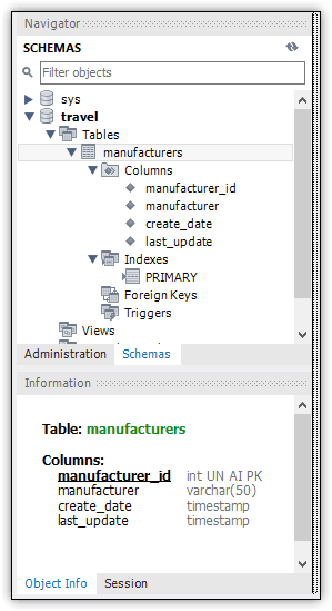
To complete the table creation process, simply click Apply and then click Finish on the next screen. You should then be able to confirm in Navigator that the table has been created, as shown in Figure 10.

The manufacturers table now visible in the Navigator under the Travel schema

Figure 10. Viewing the new table in Navigator

Notice that an index is created for the primary key column. MySQL automatically names primary key indexes PRIMARY, which might be different from what you’ve seen in other database systems. Because a table can include only one primary key, there is no problem with duplicate index names.

Using SQL to create a table in a MySQL database

The Workbench GUI features can be handy for creating database objects, especially if you’re new to MySQL or database development. They can also be useful when trying to understand the various options available when creating an object. However, most developers prefer to write the SQL code themselves, and if you already have at least some experience with SQL, you’ll likely have little problem adapting to MySQL.

With this in mind, the next step will be to create a second table in the travel database. For this, you can use the following CREATE TABLE statement:

CREATE TABLE IF NOT EXISTS airplanes (
  plane_id INT UNSIGNED NOT NULL AUTO_INCREMENT,
  plane VARCHAR(50) NOT NULL,
  manufacturer_id INT UNSIGNED NOT NULL,
  engine_type VARCHAR(50) NOT NULL,
  engine_count TINYINT NOT NULL,
  max_weight MEDIUMINT UNSIGNED NOT NULL,
  icao_code CHAR(4) NOT NULL,
  create_date TIMESTAMP NOT NULL DEFAULT CURRENT_TIMESTAMP,
  last_update TIMESTAMP NOT NULL 
    DEFAULT CURRENT_TIMESTAMP ON UPDATE CURRENT_TIMESTAMP,
  PRIMARY KEY (plane_id),
  CONSTRAINT fk_manufacturer_id FOREIGN KEY (manufacturer_id) 
    REFERENCES manufacturers (manufacturer_id) ) 
ENGINE=InnoDB AUTO_INCREMENT=101;

For the most part, the CREATE TABLE statement uses fairly standard SQL. The table is similar to the one I created in the first article in this series. It also shares some of the same elements as the manufacturers table you created above. The table includes nine columns with a mix of data types and options, although all columns are configured as NOT NULL.

One item worth pointing out is the max-weight column, which is configured with the MEDIUMINT data type (unsigned). As you’ll recall from the first article, the data type falls between SMALLINT and INT data types in terms of the supported numeric range. In this way, you have more granular options for working with integer values. Neither SQL Server nor Oracle Database support the MEDIUMINT data type.

What you haven’t seen before (at least not in this or the previous article) is the foreign key constraint that’s defined on the manufacturer_id column. The foreign key references the manufacturer_id column in the manufacturers table. The constraint ensures that any manufacturer_id value added to the airplanes table must already exist in the manufacturers table. If you try to add a different value, you’ll receive an error.

The table definition also includes two table options. The ENGINE option species InnoDB as the storage engine, and the AUTO_INCREMENT option sets the seed value to 101.

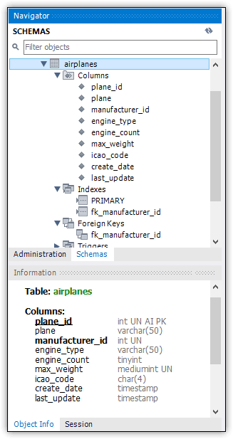
At this point, the CREATE TABLE statement should be fairly complete (at least for now), so you can go ahead and execute it in Workbench. You can then view the table in Navigator, as shown in Figure 11.

The airplanes table shown in Navigator

Figure 11. Viewing the airplanes table in Navigator

As you can see, Navigator lists the foreign key beneath the Foreign Keys node. Notice that MySQL also adds an index for the foreign key, which is assigned the same name as the foreign key. We’ll be covering indexes later in this series.

Altering a table definition in a MySQL table database

You can also use SQL to modify a table definition in MySQL. For example, the following ALTER TABLE statement adds two columns to the airplanes table:

ALTER TABLE airplanes
ADD COLUMN wingspan DECIMAL(5,2) NOT NULL AFTER max_weight,
ADD COLUMN plane_length DECIMAL(5,2) NOT NULL AFTER wingspan;

Both columns are configured with the DECIMAL(5,2) data type. This means that each column can store up to five digits with two decimal places.

Each column definition also includes an AFTER clause, which specifies where to add the column in the table definition. For example, the AFTER clause in the wingspan column definition specifies that the column should be added after the weight column, and the AFTER clause in the plane_length column definition specifies that the column should be added after the wingspan column.

When you run this ALTER TABLE statement, MySQL will update the airplanes table accordingly. You can then view the new columns in Navigator.

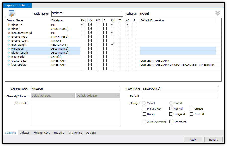
You can also use the Workbench GUI to alter a table definition. To do so, right-click the table in Navigator and then click Alter Table, which opens the Table tab. Here you can modify the column definitions or table options. You can also add or delete columns. Figure 12 shows the Table tab with the wingspan and plane_length columns selected, which are the columns you just added above.

The table properties dialog showing two new columns added, wingspan and plane_length

Figure 12. Viewing the new columns in the table editor

The next step will be to add a generated column to the table. A generated column is one in which the value is computed from an expression, similar to computed columns in SQL Server and Oracle Database.

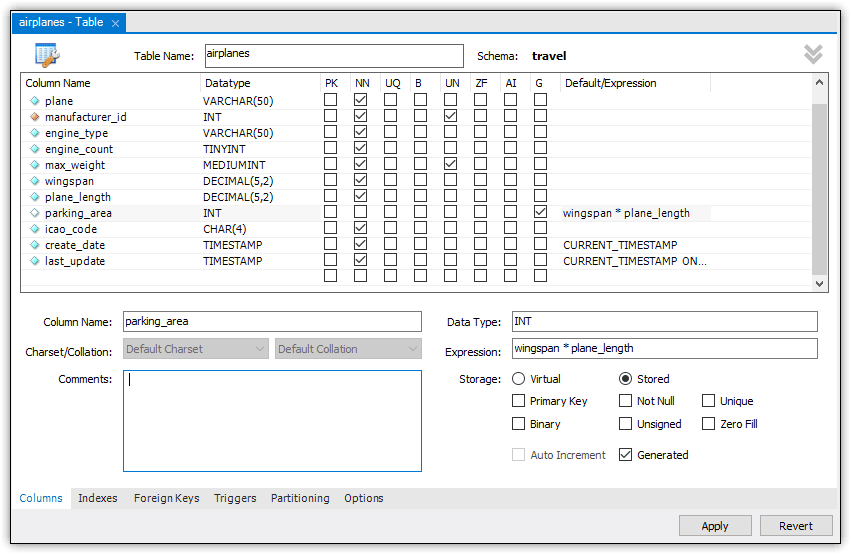
To add the column, double-click the first cell in the first empty line of the table grid (beneath the last_update column definition) and then type parking_area for the column name. On the same line, type INT for the data type, select the G option (for GENERATED), and type wingspan * plane_length in the Default/Expression column. The expression multiplies the wingspan value by the plane_length value to arrive at the total area.

When you create a generated column in the GUI, Workbench automatically selects the Virtual option in the column detail area (near the bottom of the tab). This means that the column values will be generated on demand, rather than being stored in the database. The Stored option does just the opposite. The value is calculated when a row is inserted into the table, where the value remains until the row is updated or deleted. For this article, I used the Stored option.

After you create a column, you can move it to a new location in the list of columns by dragging it to the desired position. In this case, I moved the parking_area column to after the plane_length column, as shown in Figure 13.

The edit table dialog showing the new parking_area column. Default/Expression "wingspan * plane_length". Stored and Generated are selected.

Figure 13. Adding a generated column to the airplanes table

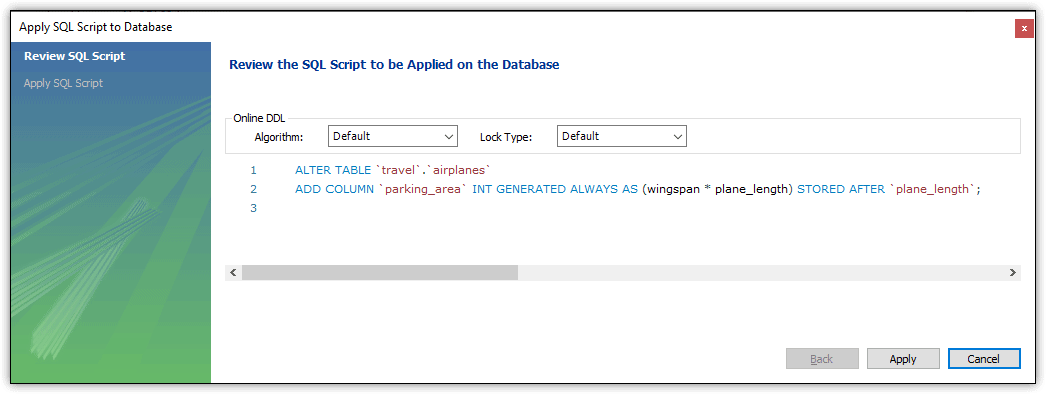
That’s all you need to do to add a generated column to the table. To complete the process, click Apply, which launches the Apply SQL Script to Database wizard. Here you can review the SQL script, as shown in Figure 14.

Dialog showing the script to add the parking_area column

Figure 14. Verifying the new column being added to the airplanes table

When Workbench generates the ALTER TABLE statement, it adds the GENERATED ALWAYS AS clause to indicate that this is a generated column. (The GENERATED ALWAYS keywords are optional and can be omitted when creating your own SQL statement.) In addition, the clause includes the computed expression, in parentheses.

Workbench also adds the STORED keyword to the column definition to indicate that the calculated values should be stored rather than computed on demand. Plus, the definition includes the AFTER clause, which indicates that the column should be added after the plane_length column.

If this all looks good to you, click Apply again and then click Finish to close the wizard. You can then confirm the table update in Navigator.

Dropping a table from a MySQL database

As with other DDL actions in Workbench, you can use SQL or the GUI to drop a table from a database. For example, you can remove the airplanes table by running the following DROP TABLE statement, which includes the optional IF EXISTS clause:

DROP TABLE IF EXISTS airplanes;

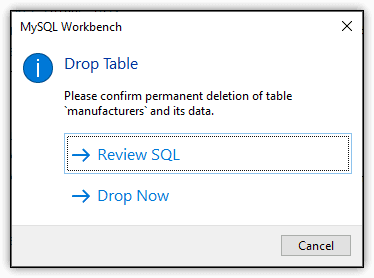
You can also drop a table through Navigator. To do so, right-click the table and then click Drop Table. This launches the Drop Table dialog box, shown in Figure 15. Click Drop Now to remove the table.

Drop table dialog. Review SQL or Drop Now

Figure 15. Deleting a table in Workbench

Notice that the dialog box also includes the Review SQL option. Click this instead if you want to review the DROP TABLE statement that Workbench has generated. You can then execute the statement from there.

Working with tables in a MySQL database

MySQL tables support a variety of options at both the column and table level, far more than can be covered reasonably in a single article. You can also create temporary tables or partition tables. You’ll find it well worth your while to review the MySQL documentation on the CREATE TABLE statement. There you can see for yourself the many ways in which you can define a MySQL table.

That said, what I’ve covered here should provide you with a good foothold for getting started with tables, whether you use SQL or the MySQL GUI. What you’ve learned here will also provide you with a foundation for working with other types of database objects, which could prove useful as we advance through this series.


The post Working with MySQL tables appeared first on Simple Talk.


from Simple Talk https://ift.tt/fQahq2A
via

Wednesday, February 23, 2022

What do employees want?

The “great resignation” is one of today’s most popular news topics. It’s an employee’s market as companies have difficulty keeping and attracting talent. Folks across the spectrum of careers give varied reasons for leaving, from seeking better benefits and pay to launching a small business they’ve always dreamed about. However, instead of blaming employees, organizations should figure out how much they are contributing to make employees leave.

I ran across an article about Elon Musk that demonstrated one of the things missing in many organizations. Love him or hate him, he’s one of the most successful people on earth. He constantly shows appreciation to his employees and teams for a job well done through email or even Twitter. I’m sure he expects a lot, but he also appreciates his teams’ efforts. I wonder if some managers think they will seem weak if they praise employees instead of constantly complaining.

Most of us have worked for organizations that expect long hours and dedication through big projects, mergers, acquisitions, migrations, and more. I remember working at places that required me to work on my regular DBA tasks early in the morning and after work, to the late hours of the night because project meetings and related tasks took up the typical day. Once during a merger, we brought two or three locations onto our systems every weekend, which meant spending Saturdays and Sundays at the office for months. (And my team leader frequently told us not to expect any comp time!) Yes, we worked hard and sacrificed family time, but management never let us know they appreciated our efforts.

What do employees want? They want to be compensated well with pay, bonuses, and benefits like healthcare and the possibility of remote work. These are great, but employees will lose heart if the organization’s culture is toxic and competitive instead of collaborative, demanding instead of encouraging, or dismissive instead of caring. Employees want chances to grow professionally and be excited about their work, and, yes, they want to know that their efforts have made a difference!

After reading the article about Elon Musk, I realized that I work for a company with a fantastic culture, and it’s positive from the CEO down. Our Slack channels are filled with notes of appreciation and encouragement, and we celebrate milestones and victories often. No organization is immune to the great resignation. Still, because Redgate values employees and fosters growth, the reasons are more likely to involve fulfilling a bucket list item than feeling unappreciated.


The post What do employees want? appeared first on Simple Talk.


from Simple Talk https://ift.tt/MVewCj0
via

The effects of NULL with NOT IN on Oracle transformations

In my first article on transformations, I described how Oracle liked to minimize the number of query blocks that the optimizer had to handle. I presented the example of an IN subquery in the where clause that Oracle would rewrite as the equivalent EXISTS subquery before unnesting the subquery to produce a join. The join might be a semi-join or partial join but might include an in-line aggregate view, which might be further transformed by complex view merging. This article considers effects of NULL with NOT IN on Oracle transformations.

There are many more transformations that the optimizer can apply to subqueries, but before moving on to any of the more subtle and complicated transformations, it’s important to look at the effects of nulls and the impact they have when IN is changed to NOT IN.

To be or not to be

Or, to relate Hamlet’s question to subqueries and the optimizer: IN or NOT IN. Before pursuing the topic of subqueries any further, it’s important to keep in mind that there is an essential difference between IN subqueries and NOT IN subqueries. While NOT EXISTS is the opposite of EXISTS, NOT IN is not the exact opposite of IN and if you forget this you may end up rewriting a query in a way that produces the wrong results.

The problem is best explained with a basic definition followed by a simple example:

  • IN() is equivalent to equals ANY()
  • NOT IN() is equivalent to not equal to ALL()

Think about what happens if the result set of your subquery includes a NULL – to keep it simple you can start with a list of values rather than a subquery then consider the two expressions:

  • 3 IN (1, 3, 5, null)
  • 4 NOT IN (1, 3, 5, null)

The first expression expands to (3 = 1) or (3 = 3) or (3 = 5) or (3 = null).

The second expression expands to (4 != 1) and (4 != 3) and (4 != 5) and (4 != null)

Because the first expression is a list of disjuncts (OR’s) it evaluates to TRUE if any of the atomic expressions evaluates to TRUE; in fact, at runtime Oracle will stop checking as soon as it finds the first expression that evaluates to TRUE (i.e. 3 = 3).

Because the second expression is a list of conjuncts (ANDs), it evaluates to TRUE only if every atomic expression evaluates to TRUE. The first three expressions evaluate to TRUE, but the last expression in the list is 4 != null, which evaluates to UNKNOWN, so the compound expression evaluates to FALSE.

To the human eye, the value 4 is clearly not in the list, but the Oracle database (or any other relational database) doesn’t interpret NOT IN the way the human eye does.

This script will build the last example into a simple Oracle model:

create table t1 (n1 number);
create table t2 (n2 number);
insert into t1 values(4);
insert into t2 values(1);
insert into t2 values(3);
insert into t2 values(5);
insert into t2 values(null);
commit;
execute dbms_stats.gather_table_stats(user,'t1')
execute dbms_stats.gather_table_stats(user,'t2')

My table t1 holds a row with the value 4, and my table t2 does not. I’m going to start by querying t1 for all the values that are IN table t2, then for all the values that are NOT IN table t2 – here are the queries with results cut and pasted from an SQL*Plus session running 19.11:

SQL> select * from t1 where n1 in (select n2 from t2);
no rows selected
SQL> 
SQL> select * from t1 where n1 not in (select n2 from t2);
no rows selected
SQL>

Whether you ask for IN or NOT IN, you get no rows – NOT IN is not the opposite of IN if the subquery can return nulls. You can confirm this point by executing two more statements:

SQL> delete from t2 where n2 is null;
1 row deleted.
SQL> 
SQL> select * from t1 where n1 not in (select n2 from t2);
        N1
----------
         4
1 row selected.

When deleting the null row from t2, the not in version of our query returns the 4 row.

Execution plans

It’s very easy to forget about the impact of nulls and the benefits of declaring mandatory columns as not null. Nulls introduce all sorts of problems (to people and to the optimizer). Over the years, the optimizer has been enhanced to work around some of the performance problems they used to produce.

Side note: Oracle handles not null column declarations differently from “(column is not null)” check constraints, and a not null declaration may allow the optimizer to consider extra execution paths that it would not otherwise be allowed to use. You may find that a simple not null declaration makes a huge difference to performance.

When looking at the execution plan from the first example with the NOT IN subquery, you can see Oracle giving a little warning about the presence of nulls and the impact it might have on our processing:

The optimizer has chosen to use a hash anti-join. The significance of the ANTI is that the test fails if the search succeeds – the predicate for operation 1 must fail for every row in t2 before the t1 row can be reported. But there’s a further label to the hash join operation: NA, for null-aware, which shows that Oracle is taking some sort of defensive action during the hash join to avoid making mistakes with nulls.

This suggests another way of understanding what’s going on. You’ve seen that IN and NOT IN aren’t exactly opposites, and you saw in the previous article that non-correlated IN subqueries could be turned into correlated EXISTS subqueries. Add the null row back into t2 and see what the execution plan looks like if you assume (incorrectly) that you can rewrite our non-correlated NOT IN subquery as a correlated NOT EXISTS subquery:

SQL> select * from t1 where not exists (select null from t2 where t2.n2 = t1.n1);
        N1
----------
         4
1 row selected.

The result from NOT EXISTS disagrees with the result from NOT IN, and the plan doesn’t quite match the NOT IN plan. Operation 1 (hash join anti) is not labeled as Null-aware (NA), and there’s a predicate at operation 3 that stops any null(s) from t2 being passed up to the hash join operation. To sum up:

  • NOT EXISTS is the opposite of EXISTS,
  • You can transform IN to EXISTS
  • You cannot (in the presence of nulls) transform NOT IN to NOT EXISTS
  • NOT IN is not (in the presence of nulls) the opposite of IN

You could get some idea of what is hidden behind the Null-Aware tag by keeping an eye open for any surprises in plans, predicates, or execution statistics.

For example, change the two tables to increase the volume of data.

create table t1 (n1, v1) as
select 
        case when rownum <= 200 then rownum end n1, 
        lpad(rownum,100) v1
from 
        all_objects
where
        rownum <= 50000
;
create table t2 as select n1 n2, v1 v2 from t1;
set serveroutput off
select /*+ gather_plan_statistics leading(t1 t2) */ 
        * 
from    t1 
where   n1 not in (select n2 from t2)
;
select  * from table(dbms_xplan.display_cursor(format=>'rowstats last'));

I’ve defined the two tables so that they both hold 50,000 rows, with only 200 rows with non-null values in each table. Here’s the execution plan I get from my query – reported from memory after executing it with rowsource execution stats enabled:

A key point to notice here is that the tablescan of t2 stopped after only 201 rows – and a couple more tests setting other rows to null show that the scan stops as soon as Oracle finds a null in t2. This makes sense of course, because as soon as Oracle finds a null in t2, the query can’t return any rows, so there’s no point in continuing.

In passing, I was a little surprised that the actual row count (A-rows) from t1 was 50,000: I had assumed before I did the test that Oracle would only build the hash table from the rows where t1.n1 was not null.

Alternative plans

After understanding Oracle’s handling of nulls and NOT IN, it’s worth taking a quick note of a couple of variations in the patterns you might see in execution plans. These variations exist because of the null-aware mechanisms as there are three possible variations with HASH JOIN ANTI operation. First, if the relevant column in the t2 (i.e. subquery) table has been defined as not null (or if you add a column is not null predicate to the subquery, you get a single null aware SNA) join:

select /*+ gather_plan_statistics leading(t1 t2) */  * from t1 where n1
not in (select n2 from t2 where n2 is not null)

Then, if you have not null declarations or predicates for the relevant columns from both tables the join becomes a normal anti join:

select /*+ gather_plan_statistics leading(t1 t2) */  * from t1 where n1
is not null and n1 not in (select n2 from t2 where n2 is not null)

Notice how the A-Rows supplied to the hash join by the t1 tablescan is just the 200 where n1 is not null in this case.

Another case which looks quite counter-intuitive appears if the statistics, indexing, and not null conditions are right:

create index t2_i2 on t2(n2);
select /*+ gather_plan_statistics */  * from t1 where  n1 is not null
and n1 not in (select n2 from t2)

I’ve added a predicate to eliminate the null rows from t1 and created an index on the n2 column of t2, and that’s had the effect of making the optimizer think that a nested loop join would be appropriate – though it is an anti join, of course, and also single null aware. However, if you look at the shape of the plan, you can see that the optimizer has started with a filter at operation 1, for which the first child is the nested loop at operation 2, and the second child is a full tablescan of t2 at operation 5. Moreover, if you look at the Starts column in the plan, you’ll see that operation 5 has started once, but operation 2 has never been started. This is an example of something I’ve labeled the fixed subquery, and it’s an example of the rare case where the last child of a filter operation can be called first to decide whether or not the first child should execute at all.

In this case, operation 1 does convert the NOT IN subquery to a NOT EXISTS subquery (I’ve expanded the predicate at operation 1 by passing the query through explain plan to show this), but this will only give the right answer if there are no rows with nulls for n2 in table t2. So the run-time activity starts with the tablescan of t2 at operation 5 to check whether or not there are any rows with n2 = null, and as you can see Oracle has found the first null, stopped the tablescan, and then not executed the nested loop.

Finally, I’ll just point out that null-awareness is not restricted to anti-joins – you may also see (S)NA on semi-joins, though the term Oracle uses, in this case, is null accepting rather than null aware. (The feature appeared in 12.1, though I have published a note about a case that produced the wrong results until12.2). The SQL has to be a little more complex (and I’ve hinted the following example fairly heavily to produce the plan I wanted from the 50,000 row tables of the previous examples):

select  /*+ 
                gather_plan_statistics 
                leading(@sel$5da710d3 t1@sel$1 t2@sel$2)
                use_nl(@sel$5da710d3 t2@sel$2)
                index(@sel$5da710d3 t2@sel$2)
        */
        * 
from    t1 
where
        n1 is null
or      exists (select null from t2 where n2 = n1)
;

The effects of NULL on Oracle optimizer transformations

You have seen IN subqueries converted to EXISTS subqueries and learned that it is not automatically safe for Oracle (or the human programmer) to convert NOT IN subqueries to NOT EXISTS subqueries thanks to problems caused by nulls in the data. In recent versions of Oracle, the optimizer has been coded to work around some of the problems, but the side effects may produce plans that have to be less efficient than you might expect and plans that might have extra operations that seem to be redundant.

Join operations with the suffix NA (null-aware/accepting) or SNA (single null-aware/accepting) are clues that the plan has been adjusted to allow for columns that may hold nulls. Therefore, it could be worth checking whether it would be legal to add is not null predicates to specific queries, or even to add NOT NULL declarations to relevant columns.


The post The effects of NULL with NOT IN on Oracle transformations appeared first on Simple Talk.


from Simple Talk https://ift.tt/K1OIsC7
via

Tuesday, February 22, 2022

The basic T-SQL SELECT statement

The SELECT statement is the most used statement in the T-SQL language. It is executed to retrieve columns of data from one or more tables. The SELECT statement can constrain the data returned by using the WHERE or HAVING clause, and sort or group results using the ORDER BY and GROUP BY clauses, respectively. A SELECT statement can also be made up of many different SELECT statements, commonly called subqueries.

There are many different aspects of the SELECT statement, making it a very complex T-SQL statement. This article is the first in a series of articles that will cover the various nuances of the SELECT statement. In this article, I will discuss only the basics of the SELECT statement.

The SELECT statement

The SELECT statement has many different pieces, making it multifaceted. The main clauses supported by the SELECT statement as found in the Microsoft Documentation are shown in Figure 1.

An image showing the many options of the SELECT statement

Figure 1: Main clauses of the SELECT statement

The SELECT statement supports many different options. To discuss each of these various options would require a very long article. For the purpose of this article, I will only be focusing on a few clauses, which I am presenting as the basic SELECT statement syntax shown in Figure 2.

An image showing the three parts: SELECT list, FROM table_source, WHERE search_condition

Figure 2: Basic SELECT statement

The basic SELECT statement has three parts: the select list, the FROM clause, and the WHERE clause.

The SELECT list

The select_list component identifies the data that will be returned when the SELECT statement is executed. This is the only part that is required in every SELECT statement. All other attributes of a SELECT statement are options.

The select_list identifies one or more items of data that will be returned when the SELECT statement is executed. When multiple items are identified in the list, each item is separated by a comma. The arguments of a select list can take on many different forms, like a column name, a calculation, a function call, or a literal constant, to name a few.

The format of the select_list as found in the SELECT clause documentation is shown in Figure 3.

An image showing many options for the SELECT list

Figure 3: Select_list specifications

Listing 1 has an example of a SELECT statement that contains only a selection list. There are two different columns of data in the list that will be returned.

Listing 1: Returning a calculated field and literal value

USE tempdb;
GO 
SELECT 1024*1024,       
       'The Basic Select Statement';

Report 1 shows the two column values returned when Listing 1 is executed.

Report 1: Columns returned when Listing 1 is executed

The first column returned is the result of a calculation that multiplies 1024 by1024. The second column displayed is just the literal string The Basic Select Statement. The columns returned were not given column names, hence why the column names say (No column name).

Not having a column name for some columns in the result set is not really a problem, unless you need to reference the returned data by name. To assign names to these two columns, a column alias can be used.

Assigning column aliases

A column alias is useful when you want to assign a specific name to a column of data returned from a SELECT statement. If you refer to the select_list specifications found in Figure 3 there are two ways to define a column alias. One way is to use the AS keyword, followed by the name of the column alias. The AS keyword is optional. The other way is to use the equal operator (=), where the alias name is defined on the left side of the = sign. The SELECT statement in Listing 2 returns the same data as Listing 1, but each item identified in the selection list has now been given a column alias name.

Listing 2: Defining column aliases

USE tempdb;
GO 
SELECT 1024*1024 AS NumOfBytesInMB,     
       'The Basic Select Statement' BasicSelectStatement;

When Listing 2 is executed each column returned will have a column alias name assigned, as shown in Report 2.

Report 2: Results from execution of Listing 2

An image showing table results: NumOfBytesInMB, BasicSelectStatement, 1048576, The Basic Select Statement

In Listing 2, both column alias names do not contain any spaces in the name. If you want to include spaces in an alias name, then the name needs to be enclosed in quotes. Quotes can either be a set of brackets or single or double quotation marks. Lisitng 3 shows how to use the different quoting options.

Listing 3: Creating alias names with spaces

USE tempdb;
GO 
SET QUOTED_IDENTIFIER ON
SELECT 1024*1024 AS [Num of bytes in a MB],     
       "Using Double Quotes" = 'The Basic Select Statement',
        'ABC' AS 'String ABC';

The output in Report 3 is produced when Listing 3 is executed.

Report 3: Aliases with spaces in name

The FROM clause

The FROM clause in SQL Server is used to identify a table or tables in which to retrieve data. In this basic SELECT clause article, I will only discuss retrieving data from a single SQL Server table. Future articles will talk about retrieving data from multiple tables.

A table within SQL Server is stored in a database. A given SQL Server instance might have many databases, and there might be many tables within a database. Tables within a database are grouped and organized by a schema. The hierarchy of databases, schemas, and tables means there might be multiple tables within a SQL Server instance that have the same name. Because a given table name could reside in various schemas, databases, or even instances, the table name used must be uniquely identified in the FROM clause. To uniquely identify a table in the FROM clause, it can be named using a one, two, three, or four-part name, where each part is separated by a period (.).

A one-part table name is a table name that doesn’t contain a period, like Orders or Customers. When a one-part name is used in the FROM clause, the database engine needs to determine which schema owns the table. To identify the schema that owns a one-part table name SQL Server uses a two-step process. The first step is to see if the table resides in the default schema associated with the user submitting the SELECT statement. If the table is in the default schema for the user, then that table is used, and the database engine doesn’t need to process the second step. If the table is not found in the user’s default schema, then the second step of identifying the table is performed. The second step looks into the dbo schema to try and find the table. When a database contains only a single schema named dbo, using one-part names makes sense. However, when there are multiple schemas in a database, it is best to use multiple part table names to clarify what table is used. It simplifies the amount of work SQL Server needs to perform to identify the table.

A two-part name is made up of both the table name and schema that contains the table with a period (.) in between, like Sales.Orders, or Sales.Customer. When writing SELECT statements that only query data from tables in a single database with multiple schemas, the best practice is to use two-part table names.

In most cases, when a SELECT statement uses tables in a single database, one and two-part table names are used. Three-part table names are needed when code is run in the context of one database and needs to retrieve data from another database, or you are joining data from multiple tables that live in different databases. The third part of the name precedes the two-part table name and identifies the database in which the table lives, like AdventureWorks2019.Sales.Orders.

The last way to uniquely identify a table in the FROM clause is to include the instance name as the fourth part. The instance name is placed in front of the fully qualified three-part table name. Four-part names are used to query across instances using a linked server. Discussion of Linked servers is an entirely separate topic, which I will leave for a future article.

The SELECT statement example in Listing 4 runs in the context of the AdventureWorks2019 database using a two-part table name to return all the data in the Territory table, owned by the Sales schema.

Listing 4: Using two-part table name

USE AdventureWorks2019;
GO
SELECT * FROM Sales.SalesTerritory;

The statement in Listing 5 uses a three-part table name to return all the data from the Territory table in the Sales schema within the AdventureWorks2019 database, but it runs in the context of the tempdb database.

Listing 5: Using three-part table name

USE tempdb
GO
SELECT * FROM AdventureWorks2019.Sales.SalesTerritory;

The rows displayed in Report 4 are produced when either the code in Listing 4 or Listing 5 is executed.

Report 4: Output when Listing 4 or 5 is run

An image showing tabular results of querying all the columns of the Sales.SalesTerritory table

In Listing 4 and Listing 5, the * wildcard character was used for the select_list option. The * tells SQL Server that all columns from the AdventureWorks2019.Sales.SalesTerritory table are to be returned based on their ordinal positions within the table. Using the * wildcard character in the selection list is a simple way to specify and select all the columns in a table. I wouldn’t recommend using wildcard characters for production code because if columns are added or dropped from the table being queried, the number of columns returned will be based on the table definition at the time of the query. Best practice is not to use wild card characters and instead specifically identify column names for the data that needs to be returned. Note that there are some situations where wildcards do make sense, and I’ll cover those in later articles. The SELECT statement in Listing 6 returns the same results as Listings 4 and 5 but specifics the actual quoted column names instead of the * wildcard character.

Listing 6: Specify column names

USE AdventureWorks2019;
GO
SELECT [TerritoryID],
       [Name], 
          [CountryRegionCode], 
          [Group], 
          [SalesYTD], 
          [SalesLastYear], 
          [CostYTD], 
          [CostLastYear], 
          [rowguid], 
          [ModifiedDate]
FROM Sales.SalesTerritory;

The WHERE clause

The SELECT statement examples I have shown so far returned all the rows in the AdventurewWorks2019.Sales.SalesTerritory table. There might be times when you don’t want to return all the rows in a table but instead only want to return a subset of rows. When this is the case, the WHERE clause can be used to restrict the rows returned.

When using the WHERE clause, search criteria needs to be specified. The search criteria identifies one or more expressions, known as predicates, that each row must meet in order to be selected. The logical operators AND, OR, and NOT can be used to string together multiple expressions for fine-tuning the exact rows that should be returned.

Listing 7 has a SELECT statement that contains a single expression in the WHERE clause. In this case, only the Sales.SalesTerritory records that have their SalesLastYear value greater than 3,000,000 will be returned.

Listing 7: Simple search condition in WHERE statement

USE AdventureWorks2019;
GO
SELECT * FROM Sales.SalesTerritory
WHERE SalesLastYear > 3000000;

When the code in Listing 6 is executed the rows in Report 5 are returned.

Report 5: Rows returned when Listing 7 is executed

An image showing tabular results. Only 6 rows returned because of the WHERE clause

Sometimes more complex search conditions are needed to produce a specific subset of rows. The SELECT statement in Listing 8 uses two different conditions in the WHERE clause to narrow down the rows returned. The two different conditions use the logical AND operator to create a complex compound search condition.

Listing 8: Using two expressions with the AND operator

USE AdventureWorks2019;
GO
SELECT * FROM Sales.SalesTerritory
WHERE SalesLastYear > 3000000
  AND CountryRegionCode = 'CA';

Report 6 shows the output created when Listing 8 is run.

Report 6: Results when Listing 8 is executed

An image showing tabular results. Only 1 row returned because of multiple predicate where clause

The basic T-SQL SELECT statement

The SELECT statement is the most used statement in the T-SQL language. Understanding the basics of the SELECT clause in the foundation of all other formats of the SELECT statement. Identifying columns in the selection list, tables in the FROM, and constraints in the WHERE clause will allow you to return any subset of rows from a database table. I will discuss other more complex aspects of querying SQL Server data using the SELECT statement in future articles.


The post The basic T-SQL SELECT statement appeared first on Simple Talk.


from Simple Talk https://ift.tt/JhB6tzW
via

Tuesday, February 15, 2022

DAX table functions for paginated reports: Part 2

The series so far:

  1. Introduction to DAX for paginated reports
  2. How to filter DAX for paginated reports
  3.  DAX table functions for paginated reports: Part 1
  4. DAX table functions for paginated reports: Part 2

Paginated reports in Power BI make heavy use of the DAX table functions. In the previous article you revised some of the core DAX table functions-such as SUMMARIZE(), ADDCOLUMNS() and GROUPBY(). This article will refresh your knowledge of some of the remaining table functions such as:

  • UNION
  • EXCEPT
  • INTERSECT
  • CALCULATETABLE

As well as these core table functions, it also helps to understand the DEFINE, EVALUATE and MEASURE functions as well as the use of variables in DAX queries when returning data to paginated reports, so the article reviews these also.

Once again, it is worth remembering that many of the DAX table functions have quirks and limitations that can trip up the unwary user in certain circumstances. However, the aim in this article is not to provide an exhaustive discussion of every available function and the hidden depths and rarer aspects of each one. Rather, the intention is to provide paginated report developers with an initial overview of the core tools that you will inevitably need to extract data for paginated reports from a Power BI dataset. This article will use the same sample file (CarsDataWarehouse.Pbix) that you saw in the previous articles in this short collection.

DAX Variables

Delivering more complex (or refined, if you prefer) output with DAX will inevitably involve the use of DAX variables. So now is a good time to introduce you to, or remind you about, DAX Variables. The first thing to remember is that DAX variables can contain:

  • Scalar values
  • Measures
  • Tables (even single row tables)
  • Variable measures (sometimes called Query Measures)

What is more, any of these elements can be “hard-coded” values. This can be extremely useful for testing & debugging when your DAX starts getting more complex.

Variables can be introduced at any point in the course of a DAX EVALUATE statement. However, for clarity, reusability and sheer elegance I often find it easier to specify variables at the top of the script using the DEFINE keyword, then use them as required inside the DAX query.

Scalar DAX variables

To get a better idea of how scalar DAX variables can be used, take a look at the following code snippet (where the parameter @Make is input as Ferrari):

DEFINE
VAR CountryFilter = "France"
VAR MakeFilter = @Make
EVALUATE
SUMMARIZECOLUMNS
(
 DimVehicle[Make]
,DimVehicle[Model]
,DimGeography[CountryName]
,FILTER(VALUES(DimGeography[CountryName])
        ,DimGeography[CountryName] = CountryFilter)
,FILTER(VALUES(DimVehicle[Make])
        ,DimVehicle[Make] = MakeFilter)
)
ORDER BY DimVehicle[Make]

The complete output from this query is as shown in the following image when typing in Ferrari at the prompt:

All that this piece of DAX does is to define two variables. The first one is given a value directly, the second is passed a value from the SSRS parameter @Make. So, overall, it is worth noting that:

  • You can also pass a paginated report parameter to a DAX variable
  • The order in which the DAX variables are introduced in the DEFINE section can be important – as they must be defined in the order in which they are later used in the DAX query. While most of the time this is not an issue, it can be a factor in large and complex DAX statements.

You can, of course, add the column(s) that you are filtering on to the output if you want to verify that the filter is working as you expect.

Measures

A DAX variable can also be a measure (a calculation if you prefer) – as you can see in the following short piece of DAX:

DEFINE
VAR CountryFilter = "France"
VAR TotalCost = SUM(FactSales[CostPrice])
EVALUATE
SUMMARIZECOLUMNS
(
 DimVehicle[Make]
,DimVehicle[Model]
,DimGeography[CountryName]
,FILTER(VALUES(DimGeography[CountryName])
        ,DimGeography[CountryName] = CountryFilter)
,"Cost per Model", SUM(FactSales[CostPrice])
,"Percentage of Total Cost", SUM(FactSales[CostPrice]) / TotalCost
)

The output (shortened) is as shown in the following image:

If you are verifying the output, remember that the DAX variable TotalCost is returning the cost for all makes for all countries – and the output table is showing only cars sold in France – and so the total of the Percentage of Total Cost is not 100%.

DAX Variables for Tables –

In the context of Paginated reports, you are more than likely to come to rely on DAX table variables as a pillar of your data extraction code. A simple example of how DAX table variables can be used is shown in the following short DAX snippet:

DEFINE
VAR SalesTable = 
SUMMARIZECOLUMNS
(
 DimVehicle[Make]
,DimVehicle[Model]
,"Sales", SUM(FactSales[SalePrice])
)
EVALUATE SalesTable

The output (shortened) is as shown in the following image:

Variable Measures

Variable measures – as distinct from merely attributing a measure to a variable can be useful in a couple of ways:

  • They can simplify code structures as this approach allows you to isolate calculations from data retrieval.
  • They are a clear aid to reusability.
  • They can be very useful for the “dummy” measure that may be required to accelerate querying in the case of wide datasets.

As a simple example, the DAX shown below uses the MEASURE keyword to introduce a variable measure:

DEFINE
VAR CountryFilter = "France"
MEASURE FactSales[TotalCost] = SUM(FactSales[CostPrice])
EVALUATE
SUMMARIZECOLUMNS
(
 DimVehicle[Make]
,DimVehicle[Model]
,DimGeography[CountryName]
,FILTER(VALUES(DimGeography[CountryName])
        ,DimGeography[CountryName] = CountryFilter)
,"Total Cost", FactSales[TotalCost]
)

The output (shortened) is as shown in the following image:

Be aware, however, that a variable measure:

  • Has to be associated with a table
  • Must be referred to using a fully qualified reference to the table and the measure.

EXCEPT, UNION and INTERSECT

As befits a data manipulation language, DAX includes three core table functions that you can use for set-based data manipulation. These are:

  • EXCEPT()
  • UNION()
  • INTERSECT()

I assume that the concepts behind these functions are self-evident, so prefer to show one way that a couple of them can be useful to resolve certain common reporting challenges. For instance, you can apply EXCEPT() and UNION() to isolate certain records (which you analyse in detail) from all the remaining records (which you aggregate into a single row in the output table).

The principle behind the query that you are about to see is:

  • Firstly, define an initial table by applying the core filters to return only the required data.
  • Secondly, from this initial dataset (which is passed to a DAX table variable) extract two separate table variables:
    • One containing the main data, aggregated by selected colours (the “detail” dataset).
    • One that aggregates all the remaining records into a single record.
  • Finally, output the two subsidiary datasets (selected group and other records aggregated into a single record) as a single table.

Here, then, is the actual code:

DEFINE
VAR SrcTable =   // The core data table containing all records
SUMMARIZECOLUMNS(
 DimVehicle[Color]
,"Total", COUNTX(FactSales, FactSales[SalePrice])
)
VAR FullList =   // The selected group of records to isolate
SUMMARIZE
(
  FILTER
  (
  SrcTable
  ,DimVehicle[Color] IN 
        {"Black", "Blue", "British Racing Green", "Green"}
  )
,DimVehicle[Color]
,"Total", COUNTX(FactSales, FactSales[SalePrice])
)
VAR RemainderList =   // All other non-selected records
EXCEPT(SrcTable, FullList)
VAR GroupedRemainder =    // All other records aggregated
SUMMARIZE(
RemainderList
,"ColumnTitle", "Other"
,"Total", COUNTX(FactSales, FactSales[SalePrice])
)
EVALUATE
UNION(FullList, GroupedRemainder)   // The final output

The output (shortened) is as shown in the following image:

Of course, the set of records that is categorised (ie., not “other”) can be calculated using a more complex DAX query rather than simply being hard-coded as is the case here.

There is one main point to note here: SUMMARIZE() can be used not only to aggregate – but also to rename the element that is output. This is a useful trick when aggregating a table into a single record.

GROUPBY and SUMMARIZE

A variation on the theme above is to isolate all records that match a simple filter category, and then aggregate the others into a single record. This time, however, GROUPBY() and SUMMARIZE() are used in slightly different ways to achieve the same result. This is an example of how DAX table functions can be combined to solve certain paginated report challenges:

DEFINE
VAR SrcTable = 
SUMMARIZECOLUMNS(
 DimCLient[ClientName]
,DimCLient[IsCreditRisk]
,"Total", COUNTX(FactSales, FactSales[SalePrice])
)
VAR FullList = 
SUMMARIZE
(
  FILTER
  (
  SrcTable
  ,DimCLient[IsCreditRisk] = 0
  )
,DimCLient[ClientName]
,"Total", COUNTX(FactSales, FactSales[SalePrice])
)
VAR GroupedRemainder = 
GROUPBY
(
  FILTER
  (
  SrcTable
  ,DimCLient[IsCreditRisk] = 1
  )
,DimCLient[IsCreditRisk]
,"Total", SUMX(CURRENTGROUP(), [Total])
)
VAR GroupedRemainderOutput = 
SUMMARIZE(
GroupedRemainder
,"ColumnTitle", "Other"
,"Total", COUNTX(FactSales, FactSales[SalePrice])
)
EVALUATE
UNION(FullList, GroupedRemainderOutput)

The output (shortened) is as shown in the following image:

The points of note here are:

  • The GROUP BY actually aggregates into a single row of data – however it outputs “True” (the actual contents of the filter).
  • SUMMARIZE() can be used simply to rename output.

CALCULATETABLE

As mentioned in the previous article, nesting filter criteria rapidly becomes wearing once you start nesting multiple criteria applied using multiple FILTER() functions. A more practical approach can be to wrap a function that returns a data table inside the CALCULATETABLE() function – and apply all the required filters as filter expressions. So, in essence you are applying CALCULATE() filters – to a table.

This approach will work not only with SUMMARIZECOLUMNS() – as you saw in the previous article – but also with SELECTCOLUMNS() and GROUPBY(). The following piece of DAX uses a SELECTCOLUMNS() function to define the table that you wish to use as the source table in the CALCULATETABLE() function, and then applies any required filters as part of the CALCULATETABLE() function:

EVALUATE

CALCULATETABLE
(
SELECTCOLUMNS
(
FactSales
,"Client", RELATED(DimCLient[ClientName])
,"City", RELATED(DimGeography[Town])
,"Credit Risk", RELATED(DimCLient[IsCreditRisk])
,"Country", RELATED(DimGeography[CountryName])
,"Make", RELATED(DimVehicle[Make])
)
,DimGeography[CountryName] = "France"
,DimVehicle[Make] = "Ferrari"
,DimCLient[IsCreditRisk] = 0
)

The output is as shown in the following image:

You need to note a few key complexities if you ever adopt this approach:

  • You will need a clear understanding of the underlying data model in order to use RELATED() if you are using SELECTCOLUMNS()
  • There are many subtleties and variations on the theme of filtering data – some ideas and suggestions are given above (and in the previous article).
  • AND logic for filtering is easy when filtering this way. OR logic can be harder (and is explained in greater detail in the third and final article in this series).

Overall, this technique is best suited to simple list output. Also, it can get complex when using measures (given the intricacies of DAX context), so for this reason too is probably best used for relatively simple list output.

Filter tables in CALCULATETABLE()

CALCULATETABLE() can also be used with filter tables as well as (or instead of) simple filter elements of the kind that you just saw.

The following DAX extract creates a table variable of a list of country names and then uses the table variable as a filter element that is applied by CALCULATETABLE():

DEFINE
VAR FilterTable = 
SUMMARIZE
(
  FILTER
  (
  DimGeography, DimGeography[CountryName] in {"France", "Belgium"}
  )
,DimGeography[CountryName]
) 
EVALUATE
CALCULATETABLE(
SUMMARIZECOLUMNS(
 DimCLient[ClientName]
,DimGeography[CountryName]
,DimGeography[Town]
,"Sales" , SUM(FactSales[SalePrice])
)
,FilterTable
)

The output (shortened once again) is as shown in the following image:

In practice, this kind of approach can be more useful if the filter table is based on, say, a calculation. As an example, the following DAX sample creates a filter table that dynamically calculates the top two selling makes of car (by sales) and filters on the result:

DEFINE
VAR TopSellersTable = 
    TOPN(
        2,
        SUMMARIZECOLUMNS
        ( 
            DimVehicle[Make]
            ,"Total Sales", SUM(FactSales[SalePrice])
        ),
        [Total Sales]
        ,DESC
    )
EVALUATE
CALCULATETABLE(
SUMMARIZECOLUMNS(
 DimCLient[ClientName]
,DimGeography[Town]
,DimVehicle[Make]
,"Sales" , SUM(FactSales[SalePrice])
)
,TopSellersTable
)

Part of the output from this code snippet is as shown in the following image:

Here too, you do not have to display the make in the output, but I have chosen to do so to prove that the filter table actually works.

ADDMISSINGITEMS

While we may have looked at the core, everyday use of SUMMARIZECOLUMNS() in the previous article, there are a couple of ways that this function can be extended that are worth knowing about. You may, one day need to use the ADDMISSINGITEMS() function to force rows to be returned that SUMMARIZECOLUMNS() would otherwise exclude.

This option of SUMMARIZECOLUMNS() forces the output of records (rows of data) that would not otherwise be returned by SUMMARIZECOLUMNS() when output rows otherwise equate to empty or Null. This is probably best appreciated using a simple example. The following code wraps a SUMMARIZECOLUMNS() function inside an ADDMISSINGITEMS() function – and specifies that the date and make should nonetheless be returned if the row is otherwise empty:

EVALUATE
ADDMISSINGITEMS
(
DimDate[FullYear]
,SUMMARIZECOLUMNS
(
 DimDate[FullYear]
,DimVehicle[Make]
,FILTER(VALUES(DimVehicle[Make]), DimVehicle[Make] = "Trabant")
,"Total", SUM(FactSales[SalePrice])
)
,DimDate[FullYear]
)
ORDER BY DimDate[FullYear], DimVehicle[Make]

Running this code gives the following output:

To make the comparison clearer, running the DAX without ADDMISSINGITEMS gives the following output:

Conclusion

As you have learned, there is a small suite of DAX table functions that you can use to return data to paginated reports from a Power BI dataset. A good understanding of the available functions – and how they can be used, individually or together – will help you to deliver the output that you wish to display in your paginated reports.

Remember that the aim of these two articles is not to provide an exhaustive and detailed overview of all the DAX table functions. The subject is simply too large for that. However, there are many excellent resources available if you wish to delve deeper into the myriad possibilities (and arcana) of table functions. What you have seen here is that you are not limited to SUMMARIZECOLUMNS() when returning tabular output from a Power BI dataset to a paginated report, and that there are several other functions that you may find useful – or even necessary – in certain circumstances.

However, returning basic tables of data is only one step on the path to delivering paginated reports. You may well need to know a plethora of tricks and techniques to solve real-world challenges. The next article in this series introduces some of the tips that you may well need when creating paginated reports using a Power BI dataset.

The post DAX table functions for paginated reports: Part 2 appeared first on Simple Talk.


from Simple Talk https://ift.tt/ph8L9oI
via