Tuesday, March 29, 2022

Site Reliability Engineering vs. DevOps

I’m honestly not a fan of pitting concepts against one another. Our goal should be extremely simple: ensure that we’re helping our organization deliver functionality in a fast, safe manner. The precise, moment-by-moment details of this really don’t matter much. There are two major thoughts and approaches, both of which are trying to achieve the same thing: Site Reliability Engineering (SRE) and DevOps. While they have a lot in common, each one has some unique features.

Rather than try to sell you on either, let’s just discuss both and then discuss how we could decide which approach is a better fit for our organization.

Site Reliability Engineering

SRE originated within Google to deal with the challenges of software development and ongoing operations. The focus is very much on using tools to support automation of processes. However, it’s also looked on as an actual role within an organization. There must be a Site Reliability Engineer in order to successfully implement Site Reliability Engineering.

The overall purpose of SRE is on the middle word of the name, Reliability. When implementing an SRE approach, you are focused first on ensuring that you are doing whatever is necessary to keep your systems online and available. Most of the automation and testing is focused on this aspect of SRE.

SRE has several core principles that are worth noting:

  • Automation: SRE treats operations as a software problem and automates every aspect of operations from deployment to monitoring. SRE focuses first on automation which means automation is everywhere with an eye towards finding more possibilities.
  • Service Level Objectives: The engineers on an SRE team will work with other teams to define Service Level Agreements (SLA) and Service Level Indictors (SLI) that define what is needed in terms of reliability and how that can be best measured. The two are combined to produce Service Level Objectives (SLO) that use the SLI and SLA as a means of defining what must be built.
  • Monitoring: Because of the embrace of automation, distributed systems, cutting edge tooling, and all the rest that define SRE, monitoring, especially monitoring of the distributed systems, becomes a vital aspect of a successful SRE implementation. Further, you can only know you’re meeting your SLO and SLA through the use of SLI, which you obtain through monitoring.
  • Preparation: Embracing development and bring developers into the operations team in order to use their skills to help you prepare for outages is fundamental to SRE. This is all in support of ensuring reliability of the systems being developed.

If you wanted to sum up SRE in a nutshell, you could say it’s a focus on reliability that uses automation and brings in the development team to help.

DevOps

DevOps has a much more organic history, coming from multiple organizations and disciplines. The focus is absolutely on development, but it intentionally brings in every IT team, and, when done well, management and the business, all as part of a fundamental shift in how functionality is defined and deployed. The result then is a process that is much broader, but far less well defined, than SRE.

DevOps was summed up rather nicely by Donovan Brown:

DevOps is the union of people, process and products to enable continuous delivery of value to our end users

The principals of DevOps then are as follows:

  • Communication: Tearing down metaphorical walls and eliminating silos is the most fundamental aspect of implementing DevOps. The integration of multiple disciplines to enhance communication between those disciplines is at the heart of the union of people, process and products.
  • Automation: Automate everything, but especially, automate testing. The focus on automation is also foundational to ensuring that you’re eliminating silos between teams.
  • Continuous Delivery: Through the application of automation and communication, the ability to deliver software and services becomes faster as well as safer.
  • Fail Early and Often: In order to better protect production environments, DevOps encourages failure in development and other environments, early in the process. This, again, provides better protection for production environments.

Summing up DevOps, we could say it’s a focus on fast development and deployment using automation to help bring in all the other teams.

Choosing one over the other

If I were forced to pick either SRE or DevOps, which would I choose? Well, I would argue that it’s a false choice.

There is nothing within SRE that precludes continuous delivery even though it’s not one of the core tenets. There’s also nothing within SRE that would prevent you from bringing in more business involvement to help achieve reliability. The rest of SRE is very much in support of the goals of DevOps. Automation and preparation would fit very neatly within a DevOps paradigm.

Conversely, there are no dictates within DevOps that suggests you shouldn’t have SLAs, SLIs and SLOs. Just the opposite in fact. You should also implement monitoring in order to meet the requirements of automated testing and continuous delivery. While nothing in DevOps defines specific roles, there is also no exclusion that would exclude having a Site Reliability Engineer in support of your DevOps process.

In short, I don’t think you are forced to pick either of these approaches. I believe that you can adopt either, or both, with equal success. It really depends on where your problems principally lie and how best to go about addressing them within your organization.

Conclusion

If you have no challenges to either your development or operations processes at work, you can safely ignore either SRE or DevOps. However, most of us are struggling in one way or another. Since either approach could be embraced without eliminating the other, I’d suggest focusing on the things you need to fix in your environment. Then, use better communication, collaboration, testing, automation and tooling to help you address those issues.


The post Site Reliability Engineering vs. DevOps appeared first on Simple Talk.


from Simple Talk https://ift.tt/gv8aYDh
via

Monday, March 28, 2022

Azure Storage: Mapping File Shares and Powershell drives

Storage Accounts allow you to create blob containers or file shares. These are two different services provided by them, but you probably already know that. The main difference between these services is the protocol used to access them. While blob containers use REST, file shares can use REST and SMB.

This means when we use file shares we can map them directly to our file system and work with them using Windows Explorer, as any other network share.

Of course, this is an oversimplification. There are some tricks when mapping an azure file share to the local machine. If you do it wrong, it can cause a lot of trouble.

File Share Quota

Each file share has a quota. The default quota is 6GB, which is quite small. Using the file share menu you can click the option Edit Quota to change this limit.

The storage account also has a quota for all the file shares. This quota has only two possible files: 5tb or 100tb.


Creating the Mapping

Create the mapping is very easy. On the file share menu, we can select the option Connect. Azure itself will provide us with a script to create the mapping on Windows, Linux or Mac.


For windows, it’s a powershell script. We can open PowerShell ISE, copy/paste the script from the portal to ISE and execute. We will immediately have a new network mapping pointing to our file share on Azure.

There are two configuration options we can choose. Once we choose these options, the script is changed to use our choices.

Authentication: We can choose if we will use Azure AD authentication or the storage account key. Azure Authentication is way better option than the storage key. However, Azure AD doesn’t work with SMB out-of-the-box. We need to provision an Azure AD Directory Services to use Azure authentication with SMB.

Drive letter: You can choose the drive letter which will be used for the mapping on your machine.

File Share Mapping Internals

There are some interesting internal tricks related to the file share mapping. Let’s analyse this and discover how to avoid some mistakes.

It’s not your regular Network Mapping

This mapping created through the PowerShell code is not your regular network mapping. You can’t managed it using the regular tools for a network mapping. It needs to be managed using Powershell.

These mappings are called Powershell drives. You can discover more about Powershell drives on this link https://docs.microsoft.com/en-us/powershell/scripting/samples/managing-windows-powershell-drives?view=powershell-7.2

It’s specially important to remember you can’t delete or disconnect the mapping using traditional OS tools, you need to use Remove-PSDrive cmdlet in Powershell

It’s not for everyone

The mapping is created for the user who executes the script and only for this user. One example is that if you execute the script with powershell running as administrator, you will not see it in a regular windows explorer window.

Big Mistake – be aware and never do this

What gave me the idea to write this article was exactly the fact I faced a huge error when handling the mappings in a wrong way. I found almost no information about how to fix this, so here it is.

The problem: You should never attempt to delete the mappings using regular OS statements. For example:

NET USE <drive> /DELETE /YES

Is a complete error – don’t do this. I did.

When this is done, the mappings are not removed. The OS, on the other hand, becomes a bit crazy, slow. Windows explorer hangs sometimes, not understanding very well the mappings.

So, it’s just about opening powershell and executing Remove-PSDrive, right?

Unfortunately not. Powershell also goes crazy and doesn’t open anymore, showing the error message Attempt to perform the InitializeDefaultDrives operation on the FileSystem’ provider failed.

No work-around:

  • Run powershell on the prompt using the -Command parameter doesn’t work, same error
  • Windows Termminal doesn’t work, same error
  • Execute powershell as administrator or System doesn’t work. The mapping will not be there.

I end up finding the solution in a strange documentation from Microsoft. Strange because it describes a completely different reason for the error, but the solution works. 

The Solution

You need to remove the mappings directly in the registry. Using RegEdit, open the following registry key and delete the folders for each mapping: HKEY_CURRENT_USER\Software\Microsoft\Windows\CurrentVersion\Explorer\MountPoints2


The additional trick on this solution is that you need to immediately restart the machine. If you open windows explorer or powershell again, the deleted folders appear again, they are like cockroaches.

Summary

Mapping a file share on the local machine is a powerful feature, but it has some tricks and if used in a wrong way can cause complex errors

The post Azure Storage: Mapping File Shares and Powershell drives appeared first on Simple Talk.


from Simple Talk https://ift.tt/p0EDc3i
via

Wednesday, March 23, 2022

Tips and tricks with DAX table functions in paginated reports

The series so far:

  1. Introduction to DAX for paginated reports
  2. How to filter DAX for paginated reports
  3.  DAX table functions for paginated reports: Part 1
  4. DAX table functions for paginated reports: Part 2
  5. Tips and tricks with DAX table functions in paginated reports

To conclude this short set of articles on using Power BI datasets as the source of data for paginated reports, I want to outline a few classic solutions to common challenges in paginated report development with DAX.

Clearly, I cannot recount every paginated report challenge that I have ever met (or heard of) when creating reports from a Power BI dataset. However, as a report developer, it helps to be aware of some of the standard solutions to the challenges that many users encounter.

This article uses the accompanying sample data (CarsDataWarehouse.pbix) as the basis for the DAX that you will use to solve these problems.

Imitating NOT IN when filtering

One initial frustration shared by SQL developers who move to DAX is that while there is an IN operator, there is no direct NOT IN equivalent.

Fortunately, there are two solutions to this challenge that are simple and easy to apply. You can:

  • Filter using NOT …. IN. As simple as this solution is, it has left many a report developer stumped initially.
  • Use EXCEPT

To begin with, suppose that you want to filter all colours but Black, Blue, and Green. This can be done using NOT … IN, as you can see in the following DAX snippet.

EVALUATE

FILTER
(
SUMMARIZECOLUMNS
(
 DimVehicle[Make]
,DimVehicle[Model]
,DimVehicle[Color]
,"Labour Cost", SUM(FactSales[LaborCost])
)
,NOT DimVehicle[Color] IN {"Black", "Blue", "Green"}
)

You can see a sample of the output from this query in the image below:

Alternatively, you can use EXCEPT to produce a similar output – with the added advantage that this approach avoids the filter column being included in the data returned to the report. What the following piece of DAX does is to create two table variables. The first contains the elements you wish to exclude, while the second contains a full dataset. The DAX then subtracts the second dataset from the first to achieve the effect of a SQL NOT IN clause.

DEFINE
VAR ExceptionList =
SUMMARIZECOLUMNS
(       
 DimVehicle[Make]
,DimVehicle[Model]
,FILTER(VALUES(DimVehicle[Color]), DimVehicle[Color] = "Black" || DimVehicle[Color] = "Blue" || DimVehicle[Color] = "Green")
)
VAR FullList =
SUMMARIZECOLUMNS
(
 DimVehicle[Make]
,DimVehicle[Model]
)
EVALUATE
EXCEPT(FullList, ExceptionList)

The output from this query is shown below:

When testing EXCEPT queries like this one, you can add the columns that you are filtering on (Make and Model in this example) in the output initially to test the results and ensure that the query is working as expected.

Then, of course, you remove these test columns from the query.

Removing filter columns

If you are using the FILTER() function, inevitably, the filtered column will be returned as part of the output. The initial solution is not to use any of the data columns used purely to filter the output in the paginated report. However, this will increase the quantity of data that is calculated and consequently increase the load on the Power BI Service.

A more polished approach is to wrap the output in a SUMMARIZE() function to remove any extraneous data so that you are only returning data that is used in the paginated report. You can see this approach applied to the NOT … IN filter that you saw in the previous section in the following DAX snippet:

EVALUATE

SUMMARIZE
(
FILTER
(
SUMMARIZECOLUMNS
(
 DimVehicle[Make]
,DimVehicle[Model]
,DimVehicle[Color]
)
,NOT DimVehicle[Color] IN {"Black", "Blue", "Green"}
)
,DimVehicle[Make]
,DimVehicle[Model]
,"Labour Cost", SUM(FactSales[LaborCost])
)

The output from this query is:

It is worth noting that you do not have to repeat any calculations (such as the Labour Cost in this example) inside the definition of the core data defined by the SUMMARIZECOLUMNS() function (although adding them here as well will not cause any effect on the output).

Custom selections in a multi-select SSRS parameter list

DAX can also be used to pre-select multiple elements in a multi-value parameter instead of entering them manually in Power BI Report Builder. This approach has the advantage of making the preselection code-based (and so easier and faster to update in the case of larger lists). You can see this in the following DAX snippet, which uses the DATATABLE() function. The entire piece of DAX is then used as the dataset that defines the selected values for the report parameter.

DEFINE
VAR OptionList = 
DATATABLE(
"Make", STRING,
   {
    {"Bentley"},
    {"Aston Martin"},
    {"Rolls Royce"},
    {"Jaguar"},
    {"Ferrari"}
   }
)
EVALUATE
OptionList

The result of this simple query is a short list of chosen elements that you subsequently use in Power BI Report Builder as the data source for the pre-selected elements of the relevant parameter:

Complex OR filters

The dashboard analytics paradigm championed by Power BI is based on finer and finer slicing of data – in other words, layering AND filters that delve deeper into the data. Paginated reports traditionally deliver lists in this way but also maintain a separate tradition of using input parameters to offer alternative selections. You could define this as the OR alternative.

This is where some slightly inventive DAX can be required as, whereas it is easy to filter DAX using alternative values for a single column (or field if you prefer), it can be a little harder to deliver output from a Power BI dataset that amalgamates data where parameters can be from any of multiple fields without a cumulative filter effect. In other words, applying OR filters across several fields is a little tricker.

Multiple OR parameters – where all are compulsory

As a first use-case, imagine a business requirement where one element must be selected from each parameter list, and if any elements from either list are found, then the data must be returned to the report. In this case, to simplify matters:

  • The parameter is not multi-select
  • Nulls are not allowed

To make things clearer, as a practical example, you want the user to select:

  • One Make (from a parameter named Make)
  • One Country (from a parameter named Country)

And these will be used in the DAX filter to output all vehicles of the specific make or sold to the specified country.

The DAX should be something like:

DEFINE
VAR Multicriteria = 
CROSSJOIN
(
 ALL(DimGeography[CountryName])
,ALL(DimVehicle[Make])
)
VAR SelectedCriteria = 
FILTER(
 MultiCriteria
,
OR(
 DimGeography[CountryName] = @Country
,DimVehicle[Make] = @Make
)
)
VAR OrOutput = 
SUMMARIZECOLUMNS
(
 DimVehicle[Make]
,DimVehicle[Model]
,DimGeography[CountryName]
,SelectedCriteria
,"Total Sales", SUM(FactSales[SalePrice])
)
EVALUATE
OrOutput

I have left the filter columns in the output from this query so that the results make it clear that the OR filter is working as expected. You do not have to deliver these columns as part of the output when delivering final production-ready reports, of course. You can see a subset of the results (where the country variable is France and the make variable is Ferrari) below:

A simple OR query works like this:

  1. CROSSJOIN() is used to produce the Cartesian join from the fields that are used as the OR parameters. These are defined as a table variable named Multicriteria.
  2. This table variable is filtered using an OR() function to filter on either of the two filter columns and the results are attributed to a new table variable named SelectedCriteria.
  3. The SelectedCriteria table variable is used as a filter table inside the SUMMARIZECOLUMNS() function that returns the required data.

There are a few points to note when using this approach:

  • CROSSJOIN() can handle more than two input tables. You can extend this filtering approach across multiple OR columns.
  • CROSSJOIN() can be replaced with SUMMARIZECOLUMNS() – and the latter is generally more efficient if you are creating the cartesian result of multiple columns or large datasets. Indeed, you could face a timeout if the output is of any size at all. So, I do not recommend using CROSSJOIN() with more than two tables unless each table has no more than a handful of rows. You can see an example of using SUMMARIZECOLUMNS() rather than CROSSJOIN() in the following snippet of DAX:
VAR Multicriteria = 
SUMMARIZECOLUMNS
(
 DimGeography[CountryName]
,DimVehicle[Make]
,"Dummy", COUNT(FactSales[SalePrice])
)
  • Remember to add a calculated column to accelerate the output of the cartesian product when using SUMMARIZECOLUMNS() just as you would when sending output data to a paginated report.

Multiple OR filters – for single elements per filtered column

The simple OR approach that you have seen can easily be extended to handle multiple input parameters. Suppose, in this particular case, that you want to filter by any of:

  • One Make
  • Or One Country
  • Or One Customer

This will require the following approach:

  • Define each of the parameters as shown above
  • Extend the CROSSJOIN() function to encompass the Cartesian join on all the fields that will be used in the nested OR() functions.
  • Extend the DAX from the previous example to using nested OR() functions to handle more than two parameters, like this:

Specifically:

DEFINE

VAR Multicriteria = 

CROSSJOIN
(
 ALL(DimGeography[CountryName])
,ALL(DimVehicle[Make])
,ALL(DimClient[ClientName])
)

VAR SelectedCriteria = 

FILTER(
 MultiCriteria
,
OR(
   OR(
      DimGeography[CountryName] = @Country
      ,DimVehicle[Make] = @Make
      )
   ,DimClient[ClientName] = @Customer
  )
)


VAR OrOutput = 

SUMMARIZECOLUMNS
(
 DimVehicle[Make]
,DimVehicle[Model]
,DimGeography[CountryName]

,SelectedCriteria

,"Total Sales", SUM(FactSales[SalePrice])
)

EVALUATE
OrOutput

Using France as the CountryName, Ferrari as the Make and WunderKar as the ClientName, this DAX query produces the following output:

OR – with multiple inputs per parameter

A different approach is necessary if you want to apply multiple alternative filter options, and allow multiple values for each parameter. In other words, if you have multiple multi-select input parameters, then you need to adopt a slightly different solution.

Defining the parameter

The first thing to do is to handle the input from the multi-select parameter. Imagine using the same two parameters as in the previous example (Country & Make) however both are multi-select parameters this time. This implies setting up the parameter input from the paginated report with a function that will concatenate the selected values, separated by the pipe character. This means creating a function in SSRS that looks like the following code snippet:

=JOIN(Parameters!ParameterName.Value, "|")

Imagine, then, that this will result in the Country and Make variables having the following contents:

  • @Country contains Belgium|Switzerland|France
  • @Make contains Aston Martin|Ferrari

The DAX that handles these input parameters and returns data where any of the input values from either parameter are found is the following:

DEFINE
VAR InputCountry = @Country 
VAR InputMake  = @Make 
VAR Multicriteria = 
SUMMARIZECOLUMNS
(
 DimGeography[CountryName]
,DimVehicle[Make]
,"Dummy", COUNT(FactSales[SalePrice])
)
VAR SelectedCriteria = 
FILTER(
 MultiCriteria
,
OR(
 PATHCONTAINS(InputCountry, DimGeography[CountryName])
,PATHCONTAINS(InputMake, DimVehicle[Make])
)
)
VAR OrOutput = 
SUMMARIZECOLUMNS
(
 DimVehicle[Make]
,DimVehicle[Model]
,DimGeography[CountryName]
,SelectedCriteria
,"Total Sales", SUM(FactSales[SalePrice])
)
EVALUATE
OrOutput

The output returned from this query is the following:

The main difference between this approach and the previous technique is that PATHCONTAINS() is used instead of a simple equality operator. This allows the DAX to filter on the multiple elements contained in each input parameter. This code snippet also shows that you can pass the contents of a paginated report variable directly to a DAX variable.

Multiple OR parameters – where none are compulsory

As a second example of an OR filter challenge, imagine that you want to extend the previous OR query but that you do not want to make any of the parameters compulsory, and each parameter can nonetheless contain potentially multiple elements to filter on. Here the challenge arises because paginated reports do not allow for multi-select variables that can also allow NULLs.

The classic solution to this challenge is to add a <No Selection> element to the list of parameters. In essence, you must add to each parameter list a value that is not actually present in the field that will be used as a filter. You then allow the possibility of passing this value back as a filter criterion. As you are applying an OR filter, the additional value that you are adding is not present in the data, and it will have no effect on the output. You can even set this value as the default for the relevant parameter.

This is a two-stage process. Firstly, you need to add a <No Selection> (or any term that is not found in the data) element to the parameter list. Secondly, you need to create a multiple OR filter as you saw previously.

Adding <No Selection> to the parameter list

The following short piece of DAX is one way to add an added element to a parameter list. This is used to populate the multi-select parameter in SSRSDEFINE

DEFINE 
VAR MainList = 
SUMMARIZECOLUMNS
(
DimGeography[CountryName]
)
VAR NoSelectElement = {"<No Selection>"}
EVALUATE
UNION(MainList, NoSelectElement)
ORDER BY DimGeography[CountryName]

The output (that you will see in a parameter list) is the following:

You can then use the DAX that you saw previously (using the Selectedcriteria and MultiCriteria table variables) to filter the output data. Even if <No Selection> is passed as an input parameter, as this is an OR filter, <No Selection> value that is passed in as a parameter element will have no effect on the output.

A couple of points are worth noting here:

  • The variable NoSelectElement is a table containing a single row of data – all created using the DAX Row Constructor.
  • ORDER BY uses the data lineage of the first table in the UNION() function to specify the field to sort on.

Using a comma-delimited list of input values to filter the output

Although most users apply filters to narrow down the output data in a report, it is also possible to enter lists of data into a paginated report parameter to specify a precise set of output records. This approach has known limitations- most notably that there is a limit to the number of elements that can be entered as a delimited list in a report variable. Nonetheless, I have seen this kind of approach used on many occasions, so it is worth explaining here.

As far as the DAX is concerned, the credit for the following code snippet goes to a superb piece of DAX by Chris Webb that I have very slightly tweaked to adapt to suit the requirements of Paginated Report input. You can find his original code here (where the concepts behind the core DAX are explained).

What this DAX does is to take a comma-delimited string of text elements and:

  • Replaces the commas with vertical bars.
  • Creates a table of the text elements (this is the clever bit).
  • Uses this table as a filter inside a CALCULATETABLE() function.

Of course, the choice of the delimiter character is up to you. All you have to do is to enter the delimiter as the second element inside the SUBSTITUTE() function.

The code snippet is the following:

DEFINE
VAR InputList = @InputListOfElements
VAR NewInputList =
    SUBSTITUTE(
        InputList ,
        ",",
        "|"
    )
VAR CaseCount =
    PATHLENGTH (NewInputList)
VAR NumberTable =
    GENERATESERIES(1, CaseCount, 1)
VAR CustomerTable =
    GENERATE (
        NumberTable,
        VAR CurrentKey = [Value]
        RETURN
            ROW ("Key", PATHITEM (NewInputList, CurrentKey))
    )
VAR GetKeyColumn =
    SELECTCOLUMNS (CustomerTable, "Key", [Key])
VAR FilterTable =
    TREATAS (GetKeyColumn, DimCLient[CustomerID])
EVALUATE
CALCULATETABLE(
SUMMARIZECOLUMNS(
 DimCLient[ClientName]
,DimVehicle[Make]
,DimVehicle[Model]
,"Sales", SUM(FactSales[SalePrice])
)
,FilterTable
)

The major challenge here is the (undocumented) limitation on the number of characters that a paginated report variable will accept. I estimate this to be around 11,000 characters approximately. So, should you need to parse longer lists, the solution is to use several input parameters in SSRS. The multiple input parameters are then combined into one variable in the DAX that returns the final output. This can be done in DAX using a simple concatenation of DAX variables rather like the example below:

VAR INP01 = @Param01
VAR INP02 = @Param02
VAR INP03 = @Param03

VAR InputList = INP01 & "," & INP02 & "," & INP03

Alternatively, you can combine the variables using SSRS code by setting the input variable for the dataset as a function using code like the following:

=Parameters!Param01.Value & IIF(IsNothing(Parameters!Param02.Value), "", "," & Parameters!Param02.Value) & IIF(IsNothing(Parameters!Param03.Value), "", "," & Parameters!Param03.Value)

While going beyond the classic approaches to reporting, this simple evolution of paginated report parameter selection opens up a range of possibilities for report data selection.

Pass RSCustomDaxFilter output to a table variable

One frustrating limitation to the RSCustomDaxFilter function is that it cannot be used twice with the same input variable inside the same DAX code block. Yet there will inevitably be times when you need to reuse the multiple filter elements to shape certain data outputs. One solution to this challenge is to use RSCustomDaxFilter to populate a table variable. This table variable can then be reused as a filter table inside a CALCULATETABLE() function. Indeed, you may prefer this technique as a coding approach for its elegance and versatility, even if you only need to use the elements in a multi-value parameter in DAX.

You can see this approach applied in the following short piece of DAX:

DEFINE
VAR FilterTable = 
SUMMARIZECOLUMNS(
RSCustomDaxFilter(@Make,EqualToCondition,[DimVehicle].[Make],String)
)
EVALUATE
CALCULATETABLE(
SUMMARIZECOLUMNS(
DimCLient[ClientName]
,DimGeography[CountryName]
)
,FilterTable
)

You need to be aware that this code snippet will not run in DAX Studio as the RSCustomDaxFilter() function is specific to SSRS. So you will have to test it inside a real SSRS report created using Power BI Report Builder.

Alternative input

One paginated report UI requirement that surfaces fairly frequently is the capability to allow the user to select the actual parameter (and not the parameter contents) that can be used inside a query. In other words, you want to use a single query to produce different outputs depending on a user selecting one of several potential input parameters. I have seen this most frequently in cases where multiple date parameters are displayed in an SSRS report, and one date only must be specified to be used as the basis for a filter.

In this example, however (given the simplicity of the sample dataset), assume that, instead of using dates, the colour and make parameters are passed to the DAX query along with a third parameter that indicates which of these two initial parameters should filter the output.

To resume, the available parameters that are defined in the report are:

  • InputSelector – The choice of which parameter will be applied (colour or make)
  • Colour – the list of colours to filter on
  • Make – The list of makes to filter on

The actual DAX is shown immediately below, with the explanation afterwards.

DEFINE
VAR    InputSelector = @InputSelector
VAR    ColourChoice = @Colour
VAR    MakeChoice = @Make
VAR CoreTable = 
SUMMARIZECOLUMNS
(
 DimGeography[SalesRegion]
,DimGeography[CountryName]
,DimVehicle[Make]
,DimVehicle[Color]
,"Total Sales", SUM(FactSales[SalePrice])
,"No. Sales", COUNT(FactSales[SalePrice])
)
VAR SelectedColour =
ADDCOLUMNS(
FILTER(
CoreTable
,DimVehicle[Color] = ColourChoice
)
,"TableSelector", "Colour"
)
VAR SelectedMake =
ADDCOLUMNS(
FILTER(
CoreTable
,DimVehicle[Make] = MakeChoice
)
,"TableSelector", "Make"
)
VAR OutputData = 
SUMMARIZE
(
FILTER
(
UNION(SelectedColour, SelectedMake)
,[TableSelector] = InputSelector   
)
,DimGeography[SalesRegion]
,DimGeography[CountryName]
,DimVehicle[Color]
,"Total Sales", SUM(FactSales[SalePrice])
,"No. Sales", COUNT(FactSales[SalePrice])
)
EVALUATE
OutputData

Running this code in DAX studio will display the Query Parameters dialog-where I have entered:

  • Colour as the parameter to use in the query
  • Red as the colour (this will be used to filter the output)
  • Ferrari as the make (this will not be used in to filter the output)

Using these parameter settings only returns red cars-whether they are Ferraris or not, as you can see below.

How it works:

  • The SSRS variables are passed to DAX variables.
  • A table variable is created containing the required (unfiltered) output data. This table contains the two columns that could be used to filter data.
  • Two table variables (SelectedColour and SelectedMake) are created, each of which extends the initial table variable with ad added column containing the filter type (colour or make) that was used to filter the contents of the table variable.
  • The two filtered table variables are UNIONed into a fourth table variable. This table is filtered (using the added column) only to display the output using the chosen parameter type.

Notes:

  • When the TableSelector column (that is added to the table variables SelectedMake and SelectedColour) is used to filter the final OutputData table variable, the column name must be in square brackets inside the FILTER() function.
  • The SUMMARIZE() function is only required to remove the filter columns. If you want to keep the filter columns in the output, then you can remove the SUMMARIZE().
  • Alternatively, it is possible to create multiple datasets instead (one for each filter type) and have multiple tables for the output in the report – and then use the selector variable to control the visibility of objects in the actual report. However, this approach entails data being sent to the report from two or more queries – and this can be voluminous. Moreover, this alternative approach rapidly makes for a complex report if there are multiple visuals that use the alternative output data.
  • It is, of course, possible to have more than two alternative filters. All you have to do is to create multiple table variables (one for each of the alternative selections) then nest UNION() functions to aggregate all data into the OutputData table.

Final comments

While it is clearly impossible to cover every DAX challenge that you will face when developing paginated reports based on a Power BI dataset, there are some limitations that you need to be aware of – particularly before promising your clients or bosses a failsafe reporting solution.

Large dataset output

It is fair to say, at risk of extreme generalisation, that Power BI and DAX are designed to aggregate and resume data rather than deliver large amounts of list-based data to users. Consequently, you need to be aware that very wide and deep paginated reports could simply overload the Power BI service and cause timeouts.

Clearly, the definitions of what defines a “wide and deep” report are open to discussion. Equally, much will depend on the resource level that you have chosen and the stress placed on the Power BI Premium service by multiple simultaneous user requests (for dashboards and paginated reports), as well as any system configuration tweaks that you have carried out.

Nonetheless, there are limits on the amount of data that can be returned using paginated reports in Power BI, and it is important not to attempt to use an SSRS-like approach to use the Power BI service as a data export and delivery vehicle.

Large parameter list input

The paginated report interface does have its limits as far as the number of elements that can be selected from a multi-value parameter list. While no one seems to know the exact value, it’s obvious when it has been reached because a report stops functioning correctly. This is something else that has to be lived within paginated reports. The only real solutions are to apply interface tweaks such as having a hierarchy of parameters where selecting one parameter restricts the selection in a second parameter – and so on. This equates to the Power BI dashboard technique of using hierarchical slicers.

Conclusion

In this article – along with the previous articles – you have learned the core approaches needed to use DAX effectively to query Power BI datasets for paginated reports. You can now deliver these reports either as stand-alone elements accessed from Power BI workspaces (or, better still, from the Power BI App) or embedded in Power BI dashboards using the paginated report visual.

You now have, in a single platform, a wide-ranging series of options to deliver the data that your users require both as dashboards and as list-style reports. Moreover, all the varied output styles can be created from a single source of data – a Power BI data model.


The post Tips and tricks with DAX table functions in paginated reports appeared first on Simple Talk.


from Simple Talk https://ift.tt/uAdHQBn
via

Mighty Tester – Gotcha!

Commentary Competition

Enjoyed the topic? Have a relevant anecdote? Disagree with the author? Leave your two cents on this post in the comments below, and our favourite response will win a $50 Amazon gift card. The competition closes two weeks from the date of publication, and the winner will be announced in the next Simple Talk newsletter.

The post Mighty Tester – Gotcha! appeared first on Simple Talk.


from Simple Talk https://ift.tt/RNIB7YD
via

Monday, March 21, 2022

SQL Server Graph Tables – Cross Database Surprises

I was putting together some queries today, pulling data from several databases. One of these is my tables that employ graph tables in SQL Server. As I started part of the query, I used a three part name to access graph table, and used * to fetch the column names in the table (as one does when looking at a few rows from a table):

SELECT *
FROM   GraphDBName.IdentityGraph.MarketingContact;

This was greeted with:

Msg 13924, Level 16, State 1, Line 114
Select * is not permitted because it refers to a node or edge table ‘GraphDBName.IdentityGraph.MarketingContact’ which is not in the current database.

I next tried to let SQL Prompt give me the column names, which were output as:

SELECT MarketingContact.$node_id,
       MarketingContact.MarketingContactId,
       MarketingContact.RowCreatedTime,
       MarketingContact.RowLastModifiedTime
FROM   GraphDBName.IdentityGraph.MarketingContact;

This returned the following:

Msg 13923, Level 16, State 5, Line 124
Pseudocolumn ‘$node_id’ is invalid because it references a node or edge table that is not in the current database.

Msg 13923, Level 16, State 5, Line 124
Pseudocolumn ‘$node_id’ is invalid because it references a node or edge table that is not in the current database.

Msg 13923, Level 16, State 5, Line 124
Pseudocolumn ‘$node_id’ is invalid because it references a node or edge table that is not in the current database.

Msg 13923, Level 16, State 5, Line 124
Pseudocolumn ‘$node_id’ is invalid because it references a node or edge table that is not in the current database.

Msg 13923, Level 16, State 5, Line 124
Pseudocolumn ‘$node_id’ is invalid because it references a node or edge table that is not in the current database.

Why so emphatic that this is not the way that it required 5 error messages? Not sure. But either way, no go. It isn’t that it won’t work at all across databases. This code works fine:

SELECT TOP 10 MarketingContactId,  ContactId
FROM   GraphDBName.IdentityGraph.MarketingContact,
               GraphDBName.IdentityGraph.MarketingLink,
               GraphDBName.IdentityGraph.Contact
WHERE MATCH(MarketingContact-(MarketingLink)->Contact);

Just understand that if you need any of the graphDb underlying data structures, you will need to find their actual physical name and use it. I would definitely suggest never accessing these columns via any method other than the pseudocolmns for production code (because you have no way to predict the column names from dev to prod (you cannot specify the names when creating a table), but this following code does work:

SELECT TOP 10 MarketingContactId,  ContactId, 
               [$from_id_BC51BB1CD6BE4631A9101A1510560591], [$to_id_E50693D30F7E41A2B8B29BA31D020332]
FROM   GraphDBName.IdentityGraph.MarketingContact,
               GraphDBName.IdentityGraph.MarketingLink,
               GraphDBName.IdentityGraph.Contact
WHERE MATCH(MarketingContact-(MarketingLink)->Contact);

Not completely surprising, but might be a bit jarring the first time you see this (and something to know if you are using the underlying graph structures in a way that isn’t exactly desirable based on how the structures were intended to be used by their creators.


The post SQL Server Graph Tables – Cross Database Surprises appeared first on Simple Talk.


from Simple Talk https://ift.tt/ZaGJSk4
via

Saturday, March 19, 2022

Oracle subquery caching and subquery pushing

The series so far:

  1. Transformations by the Oracle Optimizer
  2. The effects of NULL with NOT IN on Oracle transformations
  3. Oracle subquery caching and subquery pushing

So far, this series has examined the shape of some of the execution plans that Oracle’s optimizer can produce when there are subqueries in the where clause. It was found that the optimizer will often “unnest” a subquery to produce a join rather than using a filtering operation that repeatedly runs the subquery.

In this installment you’ll see why you might want to stop the optimizer from unnesting some subqueries and also see a way to control where in the plan the optimizer positions each subquery, a detail of timing that can affect the overall workload quite significantly.

The examples use the emp and dept tables from the scott schema ($ORACLE_HOME/rdbms/admin/utlsampl.sql), and the demonstrations run from SQL*Plus on Oracle 19.11.

Scalar subquery caching

In case you don’t have access to an instance where you can create the scott schema, here’s a query to give you the highlights of the data.

select
        d.deptno, d.dname,
        count(sal) dept_size,
        round(avg(e.sal + nvl(e.comm,0)),2) earnings_avg
from
        dept    d,
        emp     e
where
        e.deptno(+) = d.deptno
group by
        d.deptno, d.dname
order by
        d.deptno
/


The dept table has 4 rows with a primary key on deptno. The emp table has 14 rows with a primary key on empno and a foreign key constraint to dept based on deptno. There are, however, no rows in the emp table for department 40. Both tables include a few columns that I haven’t yet mentioned.

Here’s one way to write a query to report all details about all employees who earn more than the average for their department:

I’ll just point out a couple of details about the conventions used in this query:

Because I’ve used the emp table twice in this query I’ve used the same table alias twice but added a numeric suffix to make each use unique; then I’ve used the relevant alias with every column reference

  • The query consists of two query blocks, so I’ve named each query block explicitly with a qb_name (“query block name”) hint.

Here’s the result of the query:

And here’s the execution plan that appeared by default on my instance (generated using the autotrace option from SQL*Plus):

The optimizer has decided to execute this query exactly as it is written, using a correlated subquery to filter out rows from an initial table scan of emp. Operation 2 (FILTER) calls its first child to get rows from emp then for each row in turn calls the subquery passing in the current deptno as the correlation variable (the bind variable :B1 in the Predicate Information).

Here’s an important question: how many times does the correlated subquery actually run? Is it really once for every single employee, or can Oracle find a way to avoid some of the work at runtime while still following the structure of the plan?

You’ll notice that I’ve included the /*+ gather_plan_statistics */ hint in the query. If I set serveroutput off and re-execute the query, I can make a call to dbms_xplan.display_cursor() with the allstats last format option to show the rowsource execution statistics – which look like this:

set serveroutput off
-- execute query here
select * from table(dbms_xplan.display_cursor(format=>'allstats last'));

As you can see from the Starts column for operations 4 and 5, the subquery ran only 3 times (once for each department in the emp table). This is an example of scalar subquery caching at its most effective.

Each time the correlated subquery is called session “remembers” the input value (deptno) and result (avg()) of the call in a local cache and if the subquery is called with an input that has previously been used the session gets the result from this cache rather than actually running the subquery again and, as an extra little boost, doesn’t even check the cache if the deptno for the current call is the same as the one for the immediately preceding call. This means that some queries can execute much faster than the execution plan would suggest, and that’s a good argument for blocking subquery unnesting (or even rewriting your query) if you know your data well enough to be certain that the caching feature will work in your favour. There’s a note that expands on this observation at: https://jonathanlewis.wordpress.com/2006/11/06/filter-subqueries/

There’s a threat hidden behind the benefit, though, a threat that is a side effect of the way that Oracle Corp. has implemented the caching mechanism.

For many years I used to do a demonstration where I updated one row in a much larger emp table after which a query like the one above that had previously been taking just 10 milliseconds to complete suddenly took 20 seconds of CPU time using exactly the same execution plan. The problem was that I had carefully updated a specific row in a way that “broke” the caching mechanism and resulted in the session running the subquery more than 3,000 times when it had previously been running it just 6 times.

I can’t do anything so dramatic on paper with this data set but can demonstrate the nature of the issue by recreating the data set after editing the script to modify one of the department numbers. Originally the departments were created by the statements:

insert into dept values (10, 'ACCOUNTING', 'NEW YORK');
insert into dept values (20, 'RESEARCH',   'DALLAS');
insert into dept values (30, 'SALES',      'CHICAGO');
insert into dept values (40, 'OPERATIONS', 'BOSTON');

I’m going to change this to:

INSERT INTO DEPT VALUES (310,'ACCOUNTING', 'NEW YORK');
INSERT INTO DEPT VALUES (20, 'RESEARCH',   'DALLAS');
INSERT INTO DEPT VALUES (30, 'SALES',      'CHICAGO');
INSERT INTO DEPT VALUES (40, 'OPERATIONS', 'BOSTON');

In the emp table, this means I’ve also changed three occurrences of department 10 to department 310.

With the modified data set nothing changes – except the number of times the subquery starts – here’s the plan with rowsource execution stats from the modified data:

Note that the subquery (operations 4 and 5) has now reported 5 starts rather than 3.

The reason for this is that the scalar subquery cache is based on hashing – and since hash tables are always of limited size you can end up with “hash collisions”. I’ve laboriously worked out that the hash function used by Oracle for scalar subquery caching makes 30 and 310 collide. When collisions occur the internal code for scalar subquery caching doesn’t attempt to do anything clever like creating a “hash chain”, it simply executes the subquery for the problematic second value every time it re-appears.

Department 30 appeared very early on in the initial table scan of emp so Oracle ran the subquery and cached the department number and average salary for future re-use; a few rows later department 310 appeared for the first time so Oracle ran the subquery and found that it couldn’t cache the result, and the same thing happened two more times before the end of the driving table scan: resulting in two starts more than were in the original “perfect” run.

In many cases the difference in performance may not be noticeable, but if you have some queries of this type where performance varies dramatically because of the luck of the caching effect it’s nice to understand what’s happening so that you can choose to work around the problem.

Pushing subqueries

Another feature that can affect the amount of work that takes place when a query involves a subquery is the timing of the subquery. In some cases, you may find that you can reduce the number of starts of the subquery by overriding the optimizer’s decision of where in the plan the subquery should appear; in others you may find that you can eliminate more data at an earlier point in the query and do less work overall even if the number of starts of the subquery doesn’t change.

Adding a third table from the scott schema, here’s a query that tries to identify employees of a particular salary grade by referencing the salgrade table in a subquery:

select  /*+
                qb_name(main)
                gather_plan_statistics
        */
        e.ename, e.sal, d.dname
from
        emp e, dept d
where
        d.deptno = e.deptno
and     exists  (
                select  /*+ qb_name(subq) no_unnest */
                        null
                from    salgrade s
                where   s.grade = 5
                and     e.sal between s.losal and s.hisal
        )
/

By default, Oracle has a strong tendency to run filter subqueries at the latest possible stage in the execution plan, and that’s exactly how this query behaves. Here’s the plan, with the rowsource execution stats, query block names and predicate information:

Operation 1 is the FILTER operation that says: “for each row supplied by the hash join at operation 2, start the subquery at operation 5”. Since this is a plan pulled from memory the filter predicate for operation 1 has “lost” the subquery text, of course. You can see, though, from the Query Block Name section that the original query blocks still exist, the optimizer has not transformed our subquery out of existence.

The whole of the emp data set joins to the matching dept rows before attempting to discard any data. Maybe it would be more efficient to get Oracle to test each emp row before attempting the join to dept. The mechanism for doing this is known as “subquery pushing”, and you can use the push_subq hint to force it to happen (or no_push_subq if it’s happening when you don’t want it to happen).

There are two options for the hint. It can either be put into the subquery that you want to run at the earliest possible moment, or it can go in the main query block but with the @queryblock parameter to tell Oracle which (sub)query block you want pushed. In this case I’ll add the hint /*+ push_subq(@subq) */ to the main query block, producing the following plan:

There are three important points on display here. First, although the amount of work has hardly changed and the number of starts of the subquery has not changed at all, you can see (operation 3, A-rows=1) that the number of emp rows that go into the join was reduced from 12 to just 1 which, essentially, is why the workload for this query has gone down. Secondly, because the cardinality (Rows) estimate for emp has changed so much, the optimizer has changed the join method. Finally (and the most important generic point when reading execution plans) the filter operation has disappeared, re-appearing only as a filter predicate at operation 3 although (because the plan was pulled from memory) the subquery text itself has, as in the previous example, been “lost”. In cases like this, if you’re only using the basic “first child first –move down and right” strategy for reading a plan you’ll misinterpret the plan.

The Query Block Name information shows that operation 4 represents the query block called subq. That’s the big clue showing that you need to think first about the nested loop join that is operations 1,2,3,5 and 6 (labelled MAIN) – and then worry about how to stitch the subquery that is operation 4 into that nested loop. When putting the subquery to one side and then bringing it back for later consideration, it’s easier to see that you have a nested loop from emp to dept but run the filter subquery against each emp row before joining to dept.

It’s worth noting that in this example there is a correlated subquery acting as a filter predicate against a table access operation, it is also possible for a correlated subquery to act as a filter predicate against an index operation.

Summary

This article discussed two topics – scalar subquery caching and subquery pushing. Technically, of course, neither of these is a “transformation” in that they don’t manipulate your original text to re-engineer the query blocks that need to be optimized; one of them is a built-in run-time optimization, and the other doesn’t change the query block that you’re “pushing” (or not) – even though the rest of the plan may change as a consequence of your choice.

The number of times a subquery starts can make a huge difference to the workload – you might want to subvert the optimizer’s choice because you have a better idea of how well the caching might work; conversely if you recognize that the caching benefit shows extreme variation for a critical query you might rewrite the query to work completely differently, or you might engineer a solution that guarantees you get the maximum possible benefit from the caching mechanism.

The point in a plan where a filter subquery runs can make a significant difference to the number of times it runs or to the amount of data that passes through the rest of the plan. In either case, the impact on the total workload could be enormous. When a subquery is “pushed” to run as early as possible (whether that’s by default or due to hinting) the explicit FILTER operation disappears from the plan, and the shape of the plan changes in a way that can be very misleading if you’re following the “move down and right” method of reading a plan and haven’t checked the Query Block information and Predicate Information.


The post Oracle subquery caching and subquery pushing appeared first on Simple Talk.


from Simple Talk https://ift.tt/yE9XOY8
via

Ordering a result set in SQL Server

A result set is easier to view when it’s ordered, because the data can be browsed in a meaningful way. SQL Server does not guarantee a result set is ordered unless an ORDER BY clause is used. Data can be sorted in ascending and/or descending order based on one or more columns when you use an ORDER BY clause. This articles explains different ways to use the ORDER BY clause for ordering a result set.

Syntax of the ORDER BY clause

Figure 1 contains the syntax for the ORDER BY clause as found in the Microsoft Documentation.

Graphical user interface, text, application, email Description automatically generated

Figure 1: ORDER BY syntax

Test data

This article will cover a number of examples to show the different ways to use the ORDER BY clause. Each of these examples will select data from a table named TestData. If you want to follow along and run these examples, you can created this table by using the code in Listing 1.

Listing 1: Code to create TestData table

-- Create test data
USE tempdb;
GO
CREATE TABLE TestData (
ID INT, 
CharID CHAR(2),
CityName VARCHAR(20),
StateName VARCHAR(20),
Founded SMALLINT);
--Insert rows of test data
INSERT INTO TestData VALUES
(1,'1','Seattle','Washington',1851),
(11,'11','Redmond','washington',1871),
(12,'12','Bellevue','Washington',1953),
(2,'2','Portland','oregon',1851),
(5,'5','Grants Pass','Oregon',1887),
(6,'6','Spokane','washington',1881),
(7,'7','Salem','oregon',1842),
(8,'9','Bend','Oregon',1905),
(9,'9','Tacoma','Washington',1872);

Sorting based on a single column

If a SELECT statement is run without and ORDER BY clause, SQL Server does not guarantee the record set produced in sorted order. To make sure a record set is returns data in sorted order an ORDER BY clause is needed. The code in Listing 2 does not have a ORDER BY clause, and produces the unordered results found in Report 1.

Listing 2: SELECT statement without an ORDER BY clause

SELECT StateName, CityName FROM TestData;

Report 1: Unsorted Output when Listing 2 is run.

The ORDER BY clause will sort data based on one or more columns. The code in Listing 2 selects the StateName, and CityName columns from the TestData table and sorts the results set based on the single column StateName.

Listing 3: Sort based on single column

USE tempdb;
GO
SELECT StateName, CityName From TestData
ORDER BY StateName;

Report 2 shows the results when Listing 3 is executed.

Report 2: Results created when Listing 3 is run

Report2 shows the results are sorted based only on the StateName column. The CityName column has not been sorted because the code in Listing 3 only specified to sort based on the StateName column. In order to also sort the CityName column, the code would have had to sort on that column as well. Multiple column sorts is covered later in the article.

Sorting in ascending or descending order

SQL Server supports two different sort orders: ASC, and DESC. Where ASC stands for ascending and DESC stands for descending. You can not specify ascending or descending spelled out, you can only specify the abbreviations of ASC, or DESC. When no sort order is identified in the ORDER BY clasue, like in Listing 3, SQL Server uses the default sort order which is ascending. The code in Listing 4 produces the same results as Listing 3. But in Listing 4 the code tells SQL Server to use ascending sort order, because ASC was specified after the StateName column.

Listing 4: Sort order of ASC specified

USE tempdb;
GO
SELECT StateName, CityName From TestData
ORDER BY StateName ASC;

The results could be sorted in descending order by specifying DESC next to the StateName column in the ORDER BY clause, as has been done in Listing 5.

Listing 5: Sorting results based on StateName in descending order

USE tempdb;
GO
SELECT StateName, CityName From TestData
ORDER BY StateName DESC;

The code in Listing 5 produces results shown in Report 3.

Report 3: The results from running Listing 5

You may have noticed that the StateName column contains some state names where the first character of the name is in uppercase and others in lowercase. You may be wondering why these values with similar cases where not sorted together. This is because they are sorted based on the collation of the StateName column, which, in this case, is case insensitive.

Collation setting of TestData table columns

The collation of the columns in my TestData table in tempdb is SQL_Latin1_General_CP1_CI_AS. This is because my tempdb got a collation of SQL_Latin1_General_CP1_CI_AS when it was created, and I didn’t override the collation settings when creating my TestData table. Keep in mind not every tempdb database will have the same collation SQL_Latin1_General_CP1_CI_AS. The tempdb database is created each time SQL Server starts up. The collation setting of tempdb is created based on the collation of the model database. If your tempdb collation setting is not SQL_Latin1_General_CP1_CI_AS then you might see different sorting results when running any of the code in this article. To verify the collation setting of tempdb the code in Listing 6 can be executed.

Listing 6: Display the collation of tempdb

SELECT DATABASEPROPERTYEX('tempdb','collation');

How collation affects sorting

By default, SQL Server sorts character columns based on their column collation. All the TestData table character columns have a collation of SQL_Latin1_General_CP1_CI_AS. One way to verify the column collation setting is by running the code in Listing 7.

Listing 7: Displaying collation of TestData table columns

USE tempdb;
GO
SELECT c.name, 
       c.collation_name
  FROM SYS.COLUMNS c
  JOIN SYS.TABLES t ON t.object_id = c.object_id
 WHERE t.name = 'TestData';

Report 4 shows the results when I execute the code in Listing 7. If you have a different collation, you will see different results.

Report 4: Displaying collation of TestData columns

By reviewing the collation_name column, you can see that each character data column in my TestData table has a collation of SQL_Latin1_General_CP1_CI_AS.

Overriding the sort collation default

In order to override the the default collation setting of a column being sorted the COLLATE clause can be used. Listing 8 uses the COLLATE clause to get the columns of the same case to sort together.

Listing 8: Using COLLATE clause

USE tempdb;
GO
SELECT StateName, CityName FROM TestData
ORDER BY StateName COLLATE SQL_Latin1_General_CP1_CS_AS ASC;

By comparing Report 5 with Report 3, you can see that the state names with same case values are now sorted together when the StateName column was sorted based on a collation that is case sensitive.

Report 5: Output produce when Listing 8 was executed

Sorting numeric data

You would not think that sorting numbers would be a big deal. They are not when the numbers are stored in a numeric column like the ID column found in my TestData table. When a numeric value is stored in a character column, like the CharID column in my sample data, the results may not be sorted according to numeric order. To demonstrate this, execute the code in Listing 9.

Listing 9: Sorting a character column that contains numeric data

USE tempdb;
GO
SELECT CharID, StateName, CityName FROM TestData
ORDER By CharID;

Report 6 shows the results when Listing 9 is run.

Report 6: Output from Listing 9

In Report 6, the numeric values in column CharID do not seem to be sorted correctly. Meaning the values 11, and 12 appear before the value 2. This is the correct sort order for character data, but not for numeric data. In order to get numeric data stored in a character column to sort correctly based on the numeric values, all that needs to be done is to use the CAST function in the ORDER BY clause, as shown in Listing 10.

Listing 10: Using CAST function in ORDER BY clause

USE tempdb;
GO
SELECT CharID, StateName, CityName FROM TestData
ORDER By CAST(CharID as TINYINT);

By using the CAST function to covert the CharID column to a numeric data type of tinyint, SQL Server will sort the StateName column, based on its casted numeric representation. I’ll leave it up to you to run this code to verify that data is now sorted correctly for numeric values. Listing 10 also shows how a function or expression can be used in the ORDER BY clause.

Sorting based on column alias name

Alias names are also supported by the ORDER BY clause. This is especially useful when the sort order needs to be based on concatenating a couple of columns together, as shown in Listing 11.

Listing 11: Using alias name in ORDER BY clause

USE tempdb;
GO
SELECT CityName + ', ' + StateName as 'City and State' FROM TestData 
ORDER BY 'City and State';

Report 7 shows the output when Listing 11 is executed.

Report 7: Ouput from Listing 11

Sorting based on ordinal position

The ORDER BY clause also supports sorting based on an ordinal position. An ordinal position is a numeric value that represents the column position in the set being sorted. In Listing 12, a set with two columns (StateName and CityName) is being sorted based on ordinal postion 2, which in this case is the CityName column.

Listing 12: Sorting based on ordinal position

USE tempdb;
GO
SELECT StateName, CityName FROM TestData
ORDER By 2;

When the code in Listing 12 is executed, it produces the results in Report 8.

Report 8: Output when Listing 12 is run


Sorting based on multiple columns

All the examples so far have only showed how to sort a result set based on a single column. SQL Server also supports sorting data based on multiple columns. The code in Listing 13 shows how to sort my TestData using both the StateName, and CityName columns.

Listing 13: Sorting based on multiple columns

USE tempdb;
GO
SELECT StateName, CityName FROM TestData
ORDER By StateName, CityName;

Report 9 shows the output produced when Listing 13 is run.

Report 9: Ouput from Listing 13

The data is now sorted based on StateName and CityName columns in ascending order.

Sorting data in both descending and ascending order

When sorting based on multiple columns, SQL Server allows sorting each column using a different sort order. Listing 14 displays StateName and CityName values, where StateName is sorted in descending order and CityName is sorted in ascending order.

Listing 14: Sorting multiple columns using different sort orders

USE tempdb;
GO
SELECT StateName, CityName FROM TestData
ORDER By StateName DESC, CityName ASC;

Report 10 can be used to verify that StateName and CityName are sorted in DESC and ASC order, respectively.

Report 10: Output when Listing 14 is executed

Sorting data based on columns not in select list

Columns used in the ORDER BY clause don’t have to be included in the selection list. To demonstrate this the code in Listing 15 can be run.

Listing 15: Sorting based on a column not in the selection list

USE tempdb;
GO
SELECT StateName, CityName FROM TestData
ORDER By Founded;

The output in Report 11 is generated when the code in Listing 15 is executed. These results are sorted based on the column Founded, which is not in the selection list.

Report 11: Results when Listing 15 is run

To verify the results are the order based on the Founded column value the code in Listing 16 can be run.

Listing 16: Code to identify when cities are founded

USE tempdb;
GO
SELECT Founded, StateName, CityName FROM TestData
ORDER By Founded;

I’ll leave it up to you to run the code in Listing 16 to determine the dates that each city was founded.

Using offset fetch to return a subset

The ORDER BY clause also supports returning only a subset of rows from a sorted set by using the offset fetch option. To identify the subset of rows to display an OFFSET and FETCH value needs to be identified. The OFFSET value tells how many rows in the sorted set should be skipped before rows are returned. Whereas the FETCH option identifies the number of rows to return. The code in Listing 17 shows how to use the offset fetch option of the ORDER BY clause.

Listing 17: Using the Offset Fetch Option

USE tempdb;
GO
SELECT StateName, CityName, Founded FROM TestData
ORDER BY Founded
OFFSET 2 ROWS FETCH NEXT 3 ROWS ONLY;

Report 12 shows the results when Listing 17 is executed.

Report 12: Output produced by Listing 17

The numeric value for OFFSET and FETCH options can be provided as expressions. Using an expressions and the offset fetch option is a great method of paging through a sorted set a few records at a time.

Limitations and restrictions

There are a number of limitations when using the ORDER BY clause. Below are a few of the common limitations worth noting:

The ORDER BY clause is not valid in views, inline table-valued functions, derived tables, or sub-queries unless you also use the TOP clause in your statement.

  • The combined size of all columns being sorted can not exceed 8060 bytes in length.
  • If a top-level query contains a UNION, EXCEPT or INTERSECT clause then the ORDER BY clause can only appear at the end of the statement.
  • Just like any other clause, when a table name is aliased in the FROM clause, only that table alias name can be referenced in the ORDER BY clause.

For a complete list of limitations review the limitation section in the Microsoft Documenation.

Ordering a result set

Ordering a result set in a meaningful way makes it easier to review the returned data. While sorting data seems like a simple concept, in reality there are many nuances that need to be considered when sorting data, like default sort order, column collation settings, numerical data and use of aliases to name a few. Hopefully, this article provided enough examples to help out next time a result set needs to be produced in just the right sorted order.


The post Ordering a result set in SQL Server appeared first on Simple Talk.


from Simple Talk https://ift.tt/fzGVeNy
via

Thursday, March 17, 2022

Starting My New Book – Step 1 – Prepare computer(s)

The main gist of this article is that if you are starting any project where you want to both teach a subject or benchmark algorithms, the cleaner the machine you start with, the less competition you have from other software skewing the results. The only thing I installed on my new computer was SSMS and Dropbox. For Dropbox I selectively synced my project directory only to an external hard drive to make sharing projects and backups easier. Other than that, the box will be basically clean of software that a server would not have. It is running Windows 11 Pro as the operating system. (When doing heavy testing, I will turn off Dropbox syncing too).

Clearly this is the step most of us want to do for every project we do, but it can be hard to do. Clearing off a computer you own can be tough. And using a VM is a great solution, but can be kind of pricey if you start to process lots and lots of data (and it is hard to resist the temptation of cranking it up to super-computer level.

For this project I decided to pick up a new machine to use, basing my decision on the following 3 criteria to select.

  1. Give me pretty solid, repeatable test results with the software I am testing (SQL Server 2019 and 2022)
  2. Is useful when the book has been written
  3. It doesn’t cost more than I am making for the book (this was by far the hardest of the parameters!)

My old NUC computer is 3 years old, so I figured it was time to upgrade. I also decided that this time, I would work hard to have a more “real” configuration and use one computer to edit documents (a Mac Mini), one for running SSMS and SSIS (the old NUC) and one computer configured as a server just running SQL Server (a new computer).

I searched long and hard and found 2 kinds of computers that interested me. Refurbished Xeon based workstation-powerhouses (some with 24 cores), and a newer version of the NUC. The Xeon based machines fit #1 better than the NUC in many ways. Obviously a 24 core computer would be awesome, but what turned me off was the power consumption a machine like this would likely use compared to a more consumer based computer.  That plus getting a lot of RAM and SSD disk drives was more complicated pushing me close to, and often, over my budget.

So I looked at regular desktop computers. Most of the newer machines were over my budget. I briefly considered building a new computer, but I am a relational programmer for many reasons, and my not exactly strong hardware configuration ability is one of them. So I checked into newer NUC machines.

The NUC devices are classified as gaming computers, and the one I ended up finding has solid, if perhaps old, specs for IO, with 2 1TB Pci-based SSDs, and 64GB of RAM. Its downside is that their CPUs are mobile versions, but looking at the Geekbench score, it scored a 1136 single core, and 6304 multi-core (Using Geekbench downloaded from here: https://www.geekbench.com/download/windows/). (The M1 Mac chip actually scored better, but I am running SQL Server here and getting large amounts of RAM and disk on a Mac is really not cheap.)

I didn’t go with the most recent set of NUC devices that are shipping because of condition #3. I ended up finding a NUC9i7QNX NUC 9 Ghost Skull Canyon Extreme machine, with an 6 core i7-9750H, with the aforementioned added memory and disk (the NUC devices come basically empty from Intel).

A picture containing indoor, wall, floor, computer Description automatically generated

My old NUC is to the right. I like this new size because it has large fans built into the box, and my previous device had some overheating issues when I worked it too hard… which I did.

Looking at the list of Geekbench scores here: https://browser.geekbench.com/processor-benchmarks, it is not nearly at the top, but still is solid for a computer that will likely one day be my computer I use for holding copies of my theme park pictures and serving up video files in Plex.

I used Crystal Disk Mark (https://crystalmark.info/en/download/#CrystalDiskMark) and ran some tests. The disks are Kingston SNVS1000G drives. Not the best NVMe drives, but can read and write pretty fast. If I find that some things wont work well enough, I may consider changing out the drives.

Graphical user interface, application, table, Excel Description automatically generated

On the pro side, these specs are more than twice than that of my previous NUC, which has a max read throughput of around 800 MB/S, and a Geekbench score of 712/2930 and I was able to do quite a bit on that machine that also served as my daily computer the last time I was doing benchmarks. In fact, I set out to buy a machine with a lot of free disk and a lot of RAM because the last time I was working on graphs in SQL Server, I hit “limitations” when trying to process a very large graph (I loaded all of IMDB into a database and tried to do 7 degrees of Kevin Bacon..) and hopefully I will get better results this time.

Looking at Glenn Berry’s numbers here for some of his tests: https://glennsqlperformance.com/2020/12/13/some-quick-comparative-crystaldiskmark-results-in-2020/ I give this machine a “meh plus” in power, but in most of the tests I will be doing, comparing one algorithm to another is more important than if I can crunch millions of rows per second for a very long time (the faster the better in any case, but principle #3 is pretty important!)


Next step, installing SQL Server, SSMS, Visual Studio (for SSIS), configuring everything and making sure my Red-Gate tools are up to date! Then see if the 


The post Starting My New Book – Step 1 – Prepare computer(s) appeared first on Simple Talk.


from Simple Talk https://ift.tt/GhWcZxt
via

Working with MySQL Views

The series so far:

  1. Getting started with MySQL
  2. Working with MySQL tables
  3. Working with MySQL views

Like other database management systems, MySQL lets you create views that enable users and applications to retrieve data without providing them direct access to the underlying tables. You can think of a view as a predefined query that MySQL runs when the view is invoked. MySQL stores the view definition as a database object, similar to a table object.

A view offers several advantages. It abstracts the underlying table schema and restricts access to only the data returned by the view. Applications invoking the view cannot see how the tables are structured or what other data the tables contain. In this sense, the view acts as a virtual table, adding another layer of security that hides the structure of the physical tables.

A view also helps simplify queries because it presents a less complex version of the schema. For example, an application developer doesn’t need to create detailed, multi-table joins but can instead invoke the view in a basic SELECT statement. In addition, a view’s ability to abstract schema makes it possible to modify the underlying table definitions without breaking the application.

Despite the advantages that a view offers, it also comes with a number of limitations. For instance, MySQL does not let you create an index on a view, define a trigger on a view, or reference a system or user-defined variable in the view’s query.

In addition, it’s possible to drop a table that is referenced by a view without generating an error. It’s not until a user or application tries to invoke the view that MySQL raises the alarm, which could have a severe impact on running workloads. (For a complete rundown on view restrictions and for other information about views, refer to the MySQL documentation on creating views.)

Preparing your MySQL environment

A view is a stored query that MySQL runs when the view is invoked. The query is typically a SELECT statement that retrieves data from one or more tables. Starting with MySQL 8.0.19, the query can instead be a VALUES or TABLE statement, but in most cases, a SELECT statement is used, so that’s the approach I take in this article.

Any tables that are referenced by the SELECT statement must already exist before you can create the view. Beyond that, there’s not much else you need to have in place to add a view to a database, other than to be sure you have the permissions necessary to create views and query the underlying tables (a topic I’ll be discussing in more detail later in this series).

For the examples in this article, I created the travel database and added the manufacturers and airplanes tables. These are the same tables I created and updated in the previous article in this series. To add the database and tables to your MySQL instance, you can run the following SQL code:

DROP DATABASE IF EXISTS travel;
CREATE DATABASE travel;
USE travel;
CREATE TABLE manufacturers (
  manufacturer_id INT UNSIGNED NOT NULL AUTO_INCREMENT,
  manufacturer VARCHAR(50) NOT NULL,
  create_date TIMESTAMP NOT NULL DEFAULT CURRENT_TIMESTAMP,
  last_update TIMESTAMP NOT NULL 
    DEFAULT CURRENT_TIMESTAMP ON UPDATE CURRENT_TIMESTAMP,
  PRIMARY KEY (manufacturer_id) ) 
ENGINE=InnoDB AUTO_INCREMENT=1001;
CREATE TABLE airplanes (
  plane_id INT UNSIGNED NOT NULL AUTO_INCREMENT,
  plane VARCHAR(50) NOT NULL,
  manufacturer_id INT UNSIGNED NOT NULL,
  engine_type VARCHAR(50) NOT NULL,
  engine_count TINYINT NOT NULL,
  max_weight MEDIUMINT UNSIGNED NOT NULL,
  wingspan DECIMAL(5,2) NOT NULL,
  plane_length DECIMAL(5,2) NOT NULL,
  parking_area INT GENERATED ALWAYS AS ((wingspan * plane_length)) STORED,
  icao_code CHAR(4) NOT NULL,
  create_date TIMESTAMP NOT NULL DEFAULT CURRENT_TIMESTAMP,
  last_update TIMESTAMP NOT NULL 
    DEFAULT CURRENT_TIMESTAMP ON UPDATE CURRENT_TIMESTAMP,
  PRIMARY KEY (plane_id),
  CONSTRAINT fk_manufacturer_id FOREIGN KEY (manufacturer_id) 
    REFERENCES manufacturers (manufacturer_id) ) 
ENGINE=InnoDB AUTO_INCREMENT=101;

To run these statements, copy the code and paste it into a query tab in Workbench. You can then execute the statements all at once or run them one at a time in the order they’re shown here. You must create the manufacturers table before you create the airplanes table because the airplanes table includes a foreign key that references the manufacturers table.

When you’re creating a view, it’s a good idea to test the view’s SELECT statement and then run the view after it’s created. For this, you’ll need some test data. The following two INSERT statements will add a small amount of data to the two tables, enough to get you started with creating a view:

INSERT INTO manufacturers (manufacturer)
VALUES ('Airbus'), ('Beechcraft'), ('Piper');
INSERT INTO airplanes 
  (plane, manufacturer_id, engine_type, engine_count, 
    max_weight, wingspan, plane_length, icao_code)
VALUES 
  ('A380-800', 1001, 'jet', 4, 1267658, 261.65, 238.62, 'A388'),
  ('A319neo Sharklet', 1001, 'jet', 2, 166449, 117.45, 111.02, 'A319'),
  ('ACJ320neo (Corporate Jet version)', 1001, 'jet', 2, 174165, 117.45, 123.27, 'A320'),
  ('A300-200 (A300-C4-200, F4-200)', 1001, 'jet', 2, 363760, 147.08, 175.50, 'A30B'),
  ('Beech 390 Premier I, IA, II (Raytheon Premier I)', 1002, 'jet', 2, 12500, 44.50, 46.00, 'PRM1'),
  ('Beechjet 400 (from/same as MU-300-10 Diamond II)', 1002, 'jet', 2, 15780, 43.50, 48.42, 'BE40'),
  ('1900D', 1002, 'Turboprop', 2,17120,  57.75, 57.67, 'B190'),
  ('PA-24-400 Comanche', 1003, 'piston', 1, 3600, 36.00, 24.79, 'PA24'),
  ('PA-46-600TP Malibu Meridian, M600', 1003, 'Turboprop', 1, 6000, 43.17, 29.60, 'P46T'),
  ('J-3 Cub', 1003, 'piston', 1, 1220, 38.00, 22.42, 'J3');

I’ll be discussing INSERT statements in more detail later in this series, so I won’t spend a lot of time on them here. For now, all you need to know is that the first statement adds three rows to the manufacturers table, and the second statement adds 10 rows to the airplanes table.

You can execute both statements at the same time or one at a time. You must execute them in the order specified here so you don’t violate the foreign key defined on the airplanes table. Because the foreign key is configured on the manufacturer_id column, the values in the column must first exist in the manufacturers table. Again, I’ll be digging deeper into all this later in the series.

That’s the only setup you need to do to prepare your MySQL environment so you can follow along with the examples in this article. As with the first two articles in this series, I used the MySQL Community edition on a Windows computer to build the examples. I created the examples in Workbench, which comes with the Community edition.

Creating a view in MySQL

If you reviewed the previous article in this series, you know that the Workbench GUI provides the Table tab, a handy tool for building and editing a table definition. However, the one for creating views—the View tab—is not nearly so useful. One of the biggest advantages with the Table tab, especially for beginners, is that it shows the various options available to a table definition. The View tab does not provide this advantage. It basically leaves it up to you to build the CREATE VIEW statement, just like you would on a query tab.

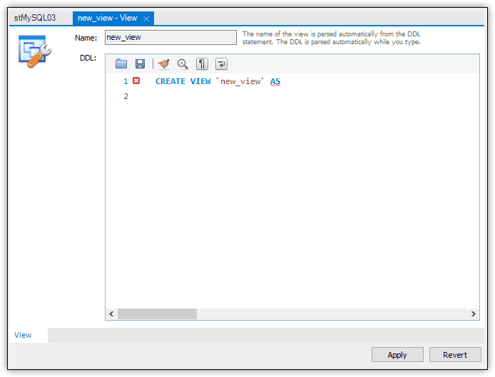
For this article, I used a query tab for all the examples. However, it’s good to know how to access the View tab in case you want to use it. To launch the tab, select the database in Navigator and then click the create view button on the Workbench toolbar. (The button is to the right of the create table icon and includes the tooltip Create a new view in the active schema in the connected server.) When you click the button, Workbench opens the View tab, as shown in Figure 1.

The create view dialog box.

Figure 1. Adding a view through the Workbench GUI

The only thing you can do in this tab is to write a CREATE VIEW statement. Although the tab provides a bit of a stub for getting started with the statement, it does not offer much else. You’re on your own to write the actual statement (or copy and paste it from another source). From there, you must then step through a couple more screens, just like you do with the Table tab, but without the benefit of an auto-generated statement.

Whether or not you use the View tab is up to you. Either way, you must still come up with the CREATE VIEW statement. With that in mind, consider the following example, which creates a view based on the two tables in the travel database:

CREATE VIEW airbus_info
AS
  SELECT a.plane, a.engine_type, a.engine_count, 
    a.wingspan, a.plane_length, a.parking_area
  FROM airplanes a INNER JOIN manufacturers m
  ON a.manufacturer_id = m.manufacturer_id
  WHERE m.manufacturer = 'airbus'
  ORDER BY a.plane;

At its most basic, the CREATE VIEW statement requires only that you specify a name for the view, followed by the AS keyword, and then followed by the SELECT statement. In this case, I’ve named the view airbus_info.

The SELECT statement itself is relatively straightforward. It defines an inner join between the airplanes and manufacturers tables, with the join based on the manufacturer_id column in each table. The WHERE clause limits the results to those rows in which the manufacturer value is airbus, and the ORDER BY clause sorts the results by the plane column.

When you’re creating a view, it’s always a good idea to run the SELECT statement on its own to ensure it’s returning the results you’re looking for. I’ve kept the statement relatively simple because I’ll be discussing SELECT statements in more detail later in this series. However, the statement I’ve used here does everything we need it to do to demonstrate how to create a view. A view’s SELECT statement can be as simple or as complex as you need it to be.

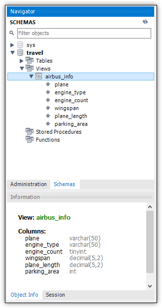
When you execute the CREATE VIEW statement, MySQL adds the view definition to the active database. You can verify that the view has been created in Navigator. You might need to refresh Navigator to see the listing, but you should find it under the Views node, as shown in Figure 2.

The Navigator showing the new view airbus_info with the columns

Figure 2. Viewing the new view in Navigator

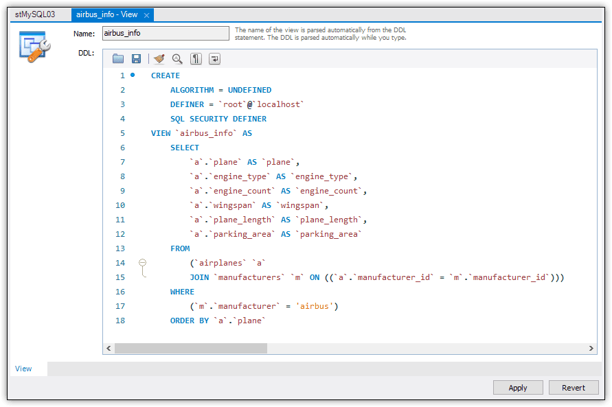
From here, you can open the view definition in the View tab. When you hover over the view’s name in Navigator, you’ll see several small icons for accessing additional features. One of these looks like a wrench. If you click this, Workbench will launch the View tab and display the view’s code, as shown in Figure 3.

The airbus_info view dialog showing the code for the view

Figure 3. Accessing the view definition through the Workbench GUI

MySQL added several options to the view definition that were not included in the original CREATE VIEW statement. The options are all configured with their default values. We’ll be discussing these options in just a bit.

You can edit the CREATE VIEW statement directly on the View tab. After you make the necessary changes, click Apply, review the code, click Apply again, and click Finish. Then close the View tab. We won’t be using this method for this article but know that it’s an option if you ever decide to go this route.

You can also open the CREATE VIEW statement on a query tab. Right-click the view in Navigator, point to Send to SQL Editor, and then click Create Statement. The statement is rendered on a single line, which is fairly unreadable. However, you can fix this by clicking the reformat button on the tab’s toolbar. (The button looks like a little broom and includes the tooltip Beautify/reformat the SQL script.)

Accessing view information through the INFORMATION_SCHEMA database

Like other relational database systems, MySQL adheres to many of the SQL standards maintained by the American National Standards Institute (ANSI). One of these standards includes the creation of the INFORMATION_SCHEMA database, which provides read-only access to details about a database system and its databases.

The information available through the INFORMATION_SCHEMA database is exposed though a set of views, one of which is named Views. Through it, you can access information about the views you create in your MySQL database. For example, the following query returns details about the view we just created in the travel database:

SELECT * FROM information_schema.views
WHERE table_schema = 'travel';

The statement uses the asterisk (*) wildcard to indicate that all columns should be returned. It also qualifies the name of the target view in the FROM clause by including the database name (information_schema), followed by a period and the name of the view (views). In addition, the statement includes a WHERE clause that filters out all views except those in the travel database.

When you run this statement, the results should include a row for the airbus_info view that you created above. The information provides details about how the view has been defined. The meaning of many of the columns in the result set should be apparent, and others I’ll be covering later in the article. But I did want to point out two columns in particular: CHECK_OPTION and IS_UPDATEABLE.

Both columns have to do with updatable views, a topic I’ll be covering later in this series. For now, just know that MySQL supports updateable views and that a view is considered updateable if it meets a specific set of criteria. MySQL automatically determines whether a view is updateable based on these criteria. If it is updateable, MySQL sets the IS_UPDATEABLE column to YES (true). Otherwise, the value is NO (false).

Another column worth noting is VIEW_DEFINITION, which contains the view’s query. If you want to view this query and nothing else, you can define your SELECT statement to limit the results:

SELECT view_definition
FROM information_schema.views
WHERE table_schema = 'travel' 
  AND table_name = 'airbus_info';

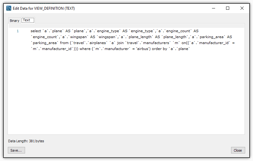
The SELECT clause now specifies that only the view_definition column be returned, rather than all columns. However, even with limiting the results, they can still be difficult to read. Fortunately, Workbench provides a handy feature for viewing a column’s value in its entirety. To access this feature, right-click the value directly in the results and click Open Value in Viewer. MySQL launches a separate window that displays the value, as shown in Figure 4.

A dialog showing the entire contents of the VIEW_DEFINITION field of the airbus_info view

Figure 4. Examining the view’s SELECT statement in Viewer

Here you can review both the binary and text values. In addition, you can save the statement to a text file by clicking the Save button. You cannot save the binary value to a file.

Querying a MySQL view

As noted earlier, I’ll be covering the SELECT statement in more detail later in this series, but I wanted to give you a quick overview of how you can query a view after it’s been created. For the most part, it works much the same way as querying a table. The following example shows a SELECT statement at its most basic, with the airbus_info view identified in the FROM clause:

SELECT * FROM airbus_info;

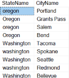
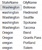
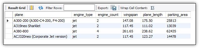
When you execute this SELECT statement, MySQL runs the query in the view definition and returns the results, just like it would if you ran the query directly. Figure 5 shows the results that your SELECT statement should return.

A grid showing the results of querying the airbus_info view. There are four rows and six columns.

Figure 5. Viewing the query results after invoking the airbus_info view

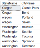
You can also refine your SELECT statement as you would when querying a view. For example, the following SELECT statement includes a WHERE clause that limits the results to those with a parking_area value greater than 20000:

SELECT * FROM airbus_info
WHERE parking_area > 20000
ORDER BY parking_area DESC;

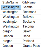
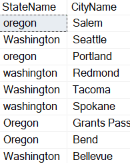
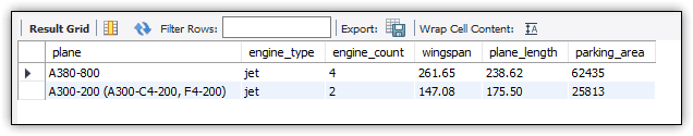
The statement also includes an ORDER BY clause that sorts the results by the parking_area column in descending order. When you include an ORDER BY clause when calling the view, it overrides the ORDER BY clause in the view definition itself (if one is included). Figure 6 shows the data that your SELECT statement should now return.

The results of running a modified query against the view. In this case, only two rows are returned.

Figure 6. Refining the query results when invoking a view

As you can see, the results now include only two rows and those rows are sorted by the values in the parking_area column, with the highest value first. The ORDER BY clause in the view definition sorts the data by the plane values.

Updating a MySQL view definition

MySQL provides several methods for modifying a view definition. One of these is to use a CREATE VIEW statement that includes the OR REPLACE clause, as shown in the following example:

CREATE OR REPLACE 
  ALGORITHM = MERGE 
  DEFINER = CURRENT_USER 
  SQL SECURITY INVOKER
VIEW airbus_info
AS
  SELECT a.plane, a.engine_type, a.engine_count, 
    a.wingspan, a.plane_length, a.parking_area
  FROM airplanes a INNER JOIN manufacturers m
  ON a.manufacturer_id = m.manufacturer_id
  WHERE m.manufacturer = 'airbus'
  ORDER BY a.plane;

By adding the OR REPLACE clause after the CREATE keyword, you can refine an existing view definition and then run the statement without generating an error, as would be the case if you didn’t include the clause. This is a great tool when you’re actively developing a database and the schema is continuously changing.

In addition to the OR REPLACE clause, the view definition includes several other elements that weren’t in the original CREATE VIEW statement that you created. The first is the ALGORITHM clause, which tells MySQL to use the MERGE algorithm when processing the view. The algorithm merges the calling statement and view definition in a way that can help make processing the view more efficient. The algorithm is also required for a view to be updatable. For more information about algorithms, see the MySQL documentation on view processing algorithms.

The other two new options—DEFINER and SQL SECURITY—control which user account privileges to use when processing the view. The DEFINER option specifies which account is designated as the view creator. In this case, the option is set to CURRENT_USER, so the definer is the user that who actually runs the CREATE VIEW statement.

The SQL SECURITY option can take either the DEFINER or INVOKER argument. If DEFINER is specified, the view will be processed under the account of the specified DEFINER. If INVOKER is specified, the view will be processed under the account of the user who invokes the view.

After you run the preceding CREATE VIEW statement, you can verify that the options have been updated by querying the view INFORMATION_SCHEMA.VIEWS:

SELECT table_name AS view_name, 
  is_updatable, definer, security_type
FROM information_schema.views
WHERE table_schema = 'travel'
  AND table_name = 'airbus_info';

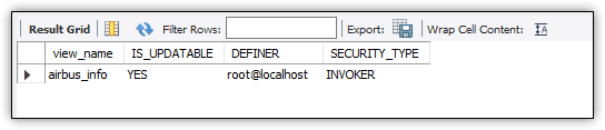
Figure 7 shows the results I received when I executed the SELECT statement on my system. Because I ran the CREATE VIEW statement as the root user, the DEFINER column shows my username, with localhost as the server instance. The results also show the INVOKER value in the SECURITY_TYPE column, which corresponds with the SQL SECURITY option.

The results of running a query to find the view properties. The DEFINER is root@localhost and SECURITY_TYPE is INVOKER

Figure 7. Viewing results from the INFORMATION_SCHEMA database

You might have noticed that INFORMATION_SCHEMA.VIEWS does not return details about the specified algorithm. In this case, however, the IS_UPDATABLE column is set to YES, indicating that the view is updatable, which works only with the MERGE algorithm. That said, if the column is set to NO, you can’t be certain which algorithm is being used because other factors might affect whether the view is updateable.

Another approach you can take to updating a view definition is to run an ALTER VIEW statement. The ALTER VIEW statement syntax is nearly the same the CREATE VIEW syntax. For example, the following ALTER VIEW statement is similar to the previous CREATE VIEW statement except that it also specifies the column names to use for the returned result set:

ALTER 
  ALGORITHM = MERGE 
  DEFINER = CURRENT_USER 
  SQL SECURITY INVOKER
VIEW airbus_info 
  (plane, engine, count, wingspan, length, area)
AS
  SELECT a.plane, a.engine_type, a.engine_count, 
    a.wingspan, a.plane_length, a.parking_area
  FROM airplanes a INNER JOIN manufacturers m
  ON a.manufacturer_id = m.manufacturer_id
  WHERE m.manufacturer = 'airbus'
  ORDER BY a.plane;

In this case, the statement includes a list of column names after the view name. The column names are enclosed in parentheses and separated by commas. These are the column names used for the view’s results, rather than using the column names of the underlying tables.

After you run the ALTER VIEW statement, you can then query the view as you did before, except that you must use the specified column names. For example, the following SELECT statement limits and orders the results, like you saw in a previous example:

SELECT plane, wingspan, length, area
FROM airbus_info
WHERE area > 20000
ORDER BY area DESC;

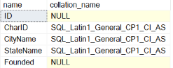
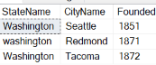
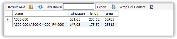
Notice that the SELECT statement uses the new column names, which are also reflected in the results, as shown in Figure 8.

The results of the view using the new column names defined by the new definition.

Figure 8. Querying the updated airbus_info view

By specifying the returned column names, you can abstract the underlying schema even further, which provides yet another level of security, while making it easier to alter the underlying table schema. For example, if you change a column name in an underlying table, you might need to update the view’s query, but not the returned column names, avoiding any disruptions to a calling application.

Dropping a MySQL view

Removing a view is a relatively straightforward process. You can use the Workbench GUI or run a DROP VIEW statement. To use the GUI, right-click the view in Navigator and click Drop View. When the Drop View dialog box appears, click Drop Now.

To use a DROP VIEW statement, you need only specify the view name and, optionally, the IF EXISTS clause, as shown in the following example:

DROP VIEW IF EXISTS airbus_info;

You can confirm that the view has been dropped by running the following SELECT statement against INFORMATION_SCHEMA.VIEWS:

SELECT * FROM information_schema.views
WHERE table_schema = 'travel';

The results should no longer include a row for the airbus_info view.

Working with views in a MySQL database

Views can provide an effective tool for presenting data to applications in a way that abstracts the underlying table structure. At the same time, they can help simplify the SQL statements that application developers need to write when retrieving data from a MySQL database. They also add an extra layer of protection by limiting access to the underlying tables.

I’ll be returning to the topic of views later in the series when I discuss querying and modifying data. Until then, the information I’ve provided in this article should give you a good starting point for working with views. As you become more adept at writing SELECT statements, you’ll be able to create more effective views that can return an assortment of information.


The post Working with MySQL Views appeared first on Simple Talk.


from Simple Talk https://ift.tt/JHb6NFk
via