Getting results using less T-SQL

While trying to solve the data challenges an organization throws our way, it is often easy to get buried in large, complex queries. Despite efforts to write concise, easy to read, maintainable T-SQL, sometimes the need to just get a data set quickly results in scary code that is better off avoided rather than committed.

This article dives into a handful of query patterns that can be useful when attempting to simplify messy code and can both improve query performance while improving maintainability at the same time!

The problems

There is no singular problem to solve here. Instead, a handful of cringeworthy T-SQL snippets will be presented, along with some alternatives that are less scary. Hopefully, this discussion not only provides some helpful solutions to common database challenges but provides some general guidance toward cleaner and more efficient code that can extend to other applications.

Note that all demos use the WideWorldImporters demo database from Microsoft.

Multiple WHERE clauses

A common need, especially in reporting, is to have to retrieve a variety of metrics from a single table. This may manifest itself in a daily status report, a dashboard, or some other scenario where intelligence about some entity is necessary. The following is an example of code that collects a variety of metrics related to orders:

SELECT
        COUNT(*) AS TotalOrderCount
FROM Sales.Orders
WHERE OrderDate >= '5/1/2016' AND OrderDate < '6/1/2016';
SELECT
        COUNT(*) AS PickingNotCompleteCount
FROM Sales.Orders
WHERE PickingCompletedWhen IS NULL
AND OrderDate >= '5/1/2016' AND OrderDate < '6/1/2016';
SELECT
        COUNT(*) PickedPersonUndefined
FROM Sales.Orders
WHERE PickedByPersonID IS NULL
AND OrderDate >= '5/1/2016' AND OrderDate < '6/1/2016';
SELECT
        COUNT(DISTINCT CustomerID) AS CustomerCount
FROM Sales.Orders
WHERE PickedByPersonID IS NULL
AND OrderDate >= '5/1/2016' AND OrderDate < '6/1/2016';
SELECT
        COUNT(*) AS ArrivingInThreeDaysOrMore
FROM Sales.Orders
WHERE DATEDIFF(DAY, OrderDate, ExpectedDeliveryDate) >= 3
AND OrderDate >= '5/1/2016' AND OrderDate < '6/1/2016';

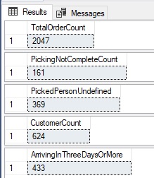
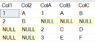
Each of these queries performs a single calculation based on order data for a specific time frame. From a reporting perspective, this is a common need. The results are as follows:

It’s a long chunk of code with many lines repeated within each query. If a change is needed in the logic behind this query, it would need to be changed in each of the five queries presented here. In terms of performance, each query takes advantage of different indexes to return its calculation. Some use index seeks and others index scans. In total, the IO for these queries is as follows:

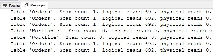
A total of 3,460 reads are required to retrieve results using two clustered index scans and three seeks. Despite the WHERE clauses varying from query to query, it is still possible to combine these individual queries into a single query that accesses the underlying table once rather than five times. This can be accomplished using aggregate functions like this:

SELECT
        COUNT(*) AS TotalOrderCount,
        SUM(CASE WHEN PickingCompletedWhen IS NULL THEN 1 ELSE 0 END) 
                  AS PickingNotCompleteCount,
        SUM(CASE WHEN PickedByPersonID IS NULL THEN 1 ELSE 0 END) 
                  AS PickedPersonUndefined,
        COUNT(DISTINCT CustomerID) AS CustomerCount,
        SUM(CASE WHEN DATEDIFF(DAY, OrderDate, ExpectedDeliveryDate) >= 3 
                 THEN 1 ELSE 0 END) AS ArrivingInThreeDaysOrMore        
FROM Sales.Orders
WHERE OrderDate >= '5/1/2016' AND OrderDate < '6/1/2016';

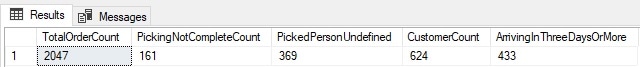
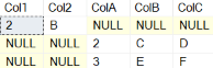
The resulting code returns the same results in a single statement, rather than five, trading more lines of code for more complex code within the SELECT portion:

In this particular scenario, the query also performs better, requiring one scan rather than two scans and three seeks. The updated IO is as follows:

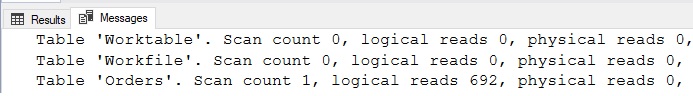
The performance of a set of queries that are combined using this method will typically mirror the performance of the worst-performing query in the batch. This will not always be an optimization, but by combining many different calculations into a single statement, efficiency can be found (sometimes). Always performance test code changes to ensure that new versions are acceptably efficient for both query duration and resource consumption.

The primary benefit of this refactoring is that the results require far less T-SQL. A secondary benefit is that adding and removing calculations can be done by simply adding or removing another line in the SELECT portion of the query. Maintaining a single query can be simpler than maintaining one per calculation. Whether or not performance will improve depends on the underlying queries and table structures. Test thoroughly to ensure that changes do indeed help (and not harm) performance.

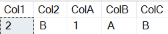
One additional note on the use of DISTINCT: It is possible to COUNT DISTINCT for a subset of rows using syntax like this:

SELECT
        COUNT(DISTINCT CASE WHEN PickingCompletedWhen IS NOT NULL 
        THEN CustomerID ELSE NULL END) AS CustomerCountForPickedItems
FROM Sales.Orders
WHERE OrderDate >= '5/1/2016' AND OrderDate < '6/1/2016';

This looks a bit clunky, but it allows a distinct count of customers to be calculated, but only when a specific condition is met. In this case, when PickingCompletedWhen IS NOT NULL.

Duplicate management

Finding (and dealing with) unwanted duplicates is quite common in the world of data. Not all tables have constraints, keys, or triggers to ensure that the underlying data is always pristine, and in lieu of that is the question of how to most easily find duplicates.

The following example shows a small data set of customers and order counts for a given date:

CREATE TABLE #CustomerData
(       OrderDate DATE NOT NULL,
        CustomerID INT NOT NULL,
        OrderCount INT NOT NULL);
INSERT INTO #CustomerData
        (OrderDate, CustomerID, OrderCount)
VALUES
        ('4/14/2022', 1, 100), ('4/15/2022', 1, 50), 
        ('4/16/2022', 1, 85), ('4/17/2022', 1, 15), 
        ('4/18/2022', 1, 125), ('4/14/2022', 2, 2), 
        ('4/15/2022', 2, 8), ('4/16/2022', 2, 7), 
        ('4/17/2022', 2, 0), ('4/18/2022', 2, 12),
        ('4/14/2022', 3, 25), ('4/15/2022', 3, 18), 
        ('4/16/2022', 3, 38), ('4/17/2022', 3, 44), 
        ('4/18/2022', 3, 10), ('4/14/2022', 4, 0), 
        ('4/15/2022', 4, 0), ('4/16/2022', 4, 1), 
        ('4/17/2022', 4, 3), ('4/18/2022', 4, 0),
        ('4/14/2022', 5, 48), ('4/15/2022', 5, 33), 
        ('4/16/2022', 5, 59), ('4/17/2022', 5, 24), 
        ('4/18/2022', 4, 90);

This data was retrieved from a handful of order systems and needs to be validated for duplicates based on order date and customer. A unique constraint is not ideal on this table as it would prevent further analysis. Instead, the validation occurs after-the-fact so that there is control over how duplicates are reported and managed.

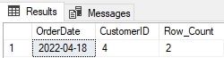
For this example, assume that when duplicates are identified, the one with the highest order count is retained and others are discarded. There are many ways to identify which rows are duplicates. For example, the data can be aggregated by OrderDate and CustomerID:

SELECT
        OrderDate,
        CustomerID,
        COUNT(*) AS Row_Count
FROM #CustomerData
GROUP BY OrderDate, CustomerID
HAVING COUNT(*) > 1;

This identifies a single OrderDate/CustomerID pair with duplicates:

Once identified, any extra rows need to be deleted, which requires a separate query to remove them. Most common methods of duplicate removal require two distinct steps:

1. Identify duplicates
2. Remove duplicates

Here is an alternative that requires only a single step to do its work:

WITH CTE_DUPES AS (
        SELECT
                OrderDate,
                CustomerID,
                ROW_NUMBER() OVER (PARTITION BY OrderDate, CustomerID 
                      ORDER BY OrderCount DESC) AS RowNum
        FROM #CustomerData)
DELETE
FROM CTE_DUPES
WHERE RowNum > 1;

Using a common-table expression combined with the ROW_NUMBER window function allows for duplicates to be identified within the CTE and immediately deleted in the same statement. The key to this syntax is that the PARTITION BY needs to contain the columns that are to be used to identify the duplicates. The ORDER BY determines which row should be kept (row number = 1) and which rows should be deleted (row numbers > 1). Replacing the DELETE with a SELECT * is an easy way to validate the results and ensure that the correct rows are getting jettisoned.

In addition to simplifying what could otherwise be some complex T-SQL, this syntax scales well as the complexity of the duplication logic increases. If more columns are required to determine duplicates or if determining which to remove requires multiple columns, each of those scenarios can be resolved by adding columns to each part of the ROW_NUMBER window function.

Code and list generation with dynamic SQL

A tool often maligned as hard to document, read, or maintain, dynamic SQL can allow for code to be greatly simplified when used effectively. A good example of this is in generating T-SQL. Consider code that performs a maintenance task on each user database on a SQL Server, such as running a full backup before a major software deployment. The most common solutions to this request would be one of these chunks of code:

-- Solution 1:
BACKUP DATABASE [AdventureWorks2017] 
TO DISK = 'D:\ReleaseBackups\AdventureWorks2017.bak';
BACKUP DATABASE [AdventureWorksDW2017] 
TO DISK = 'D:\ReleaseBackups\AdventureWorksDW2017.bak';
BACKUP DATABASE [WideWorldImporters] 
TO DISK = 'D:\ReleaseBackups\WideWorldImporters.bak';
BACKUP DATABASE [WideWorldImportersDW] 
TO DISK = 'D:\ReleaseBackups\WideWorldImportersDW.bak';
BACKUP DATABASE [BaseballStats] 
TO DISK = 'D:\ReleaseBackups\BaseballStats.bak';
BACKUP DATABASE [ReportServer] 
TO DISK = 'D:\ReleaseBackups\ReportServer.bak';
-- Solution 2
DECLARE DatabaseCursor CURSOR FOR
        SELECT databases.name 
        FROM sys.databases 
        WHERE name NOT IN ('master', 'model', 'MSDB', 'TempDB');
OPEN DatabaseCursor;
DECLARE @DatabaseName NVARCHAR(MAX);
DECLARE @SqlCommand NVARCHAR(MAX);
FETCH NEXT FROM DatabaseCursor INTO @DatabaseName;
WHILE @@FETCH_STATUS = 0
BEGIN
        SELECT @SqlCommand = N'
        BACKUP DATABASE [' + @DatabaseName + '] 
         TO DISK = ''D:\ReleaseBackups\' + @DatabaseName + '.bak'';';
        EXEC sp_executesql @SqlCommand;
        FETCH NEXT FROM DatabaseCursor INTO @DatabaseName;
END
CLOSE DatabaseCursor;
DEALLOCATE DatabaseCursor;

The first solution has database names hard-coded into backup statements. While simple enough, it requires manual maintenance as each time a database is added or removed; this code needs to be updated to be sure that databases are all getting backup up properly. For a server with a large number of databases, this could become a very large chunk of code to maintain.

The second solution uses a cursor to iterate through databases, backing each up one-at-a-time. This is dynamic, ensuring that the list of databases to backup is complete, but it uses a cursor and iterates to complete the set of backups. While a more scalable solution, it is still a bit cumbersome and relies on a cursor or WHILE loop to ensure each database is accounted for.

Consider this alternative:

DECLARE @SqlCommand NVARCHAR(MAX) = '';
SELECT @SqlCommand = @SqlCommand + N'
        BACKUP DATABASE [' + name + '] 
        TO DISK = ''D:\ReleaseBackups\' + name + '.bak'';'
FROM sys.databases
WHERE name NOT IN ('master', 'model', 'MSDB', 'TempDB');
EXEC sp_executesql @SqlCommand;

In this example, dynamic SQL is built directly from sys.databases, allowing a single T-SQL statement to generate the full list of backup commands, which are then immediately executed in a single batch. This is fast, efficient, and the smaller T-SQL is less complex than the earlier dynamic SQL example and easier to maintain than the hard-coded list of backups. This code does not speed up the backup processes themselves, but simplifies the overhead needed to manage them.

Lists can be similarly generated. For example, if a comma-separated list of names was required by a UI, it could be generated using a method like this:

DECLARE @MyList VARCHAR(MAX) = '';
SELECT
        @MyList = @MyList + FullName + ','
FROM Application.People
WHERE IsSystemUser = 1
AND IsSalesperson = 1;
IF LEN(@MyList) > 0
        SELECT @MyList = LEFT(@MyList, LEN(@MyList) - 1);
SELECT @MyList;

The results stored in @MyList are as follows:

Nothing fancy, but the ability to generate that list without an iterative loop and without extensive T-SQL is convenient. Note that the final two lines of this code serve to remove the trailing comma if the list was non-empty.

Alternatively, STRING_AGG can take the place of list-building, like this:

SELECT
        STRING_AGG(FullName,',')
FROM Application.People
WHERE IsSystemUser = 1 
AND IsSalesperson = 1;

Even less code! The dynamic SQL syntax will benefit from flexibility if there is a need to do quite a bit of string manipulation, but STRING_AGG provides the most minimalist solution possible.

Generating a list using dynamic SQL will often be an efficient and simple way to either display data in a compact format or to execute T-SQL statements en masse via metadata stored in a user table or system view. This is a scenario where dynamic SQL can simplify maintenance and also decrease the amount of code that needs to be maintained in stored procedures, PowerShell, or script files.

Reading and writing data simultaneously using OUTPUT

A common need in applications that write transactional data is to immediately retrieve and use recently modified data. The classic tactic for accomplishing this would be to:

1. Modify data
2. Determine what data was modified using temp tables, SCOPE_IDENTITY(), SELECT statements with targeted filters, or some other process.
3. Use the information from step #2 to retrieve any changed data that is required by the application.

While functionally valid, this process requires accessing transactional data multiple times to write it and then retrieving the recently written rows. OUTPUT allows recently modified data to be captured as part of the same T-SQL statement that modifies it. The following is an example of an update statement that uses OUTPUT to retrieve some metadata about which rows were updated in an inventory table:

CREATE TABLE #StockItemIDList
        (StockItemID INT NOT NULL PRIMARY KEY CLUSTERED);
UPDATE StockItemHoldings
        SET BinLocation = 'Q-1'
OUTPUT INSERTED.StockItemID
INTO #StockItemIDList
FROM warehouse.StockItemHoldings
WHERE BinLocation = 'L-3';
SELECT * FROM #StockItemIDList;
DROP TABLE #StockItemIDList;

The update is straightforward, updating an item’s location to someplace new. The added OUTPUT clause takes the IDs for all updated rows and inserts them into the temporary table. This allows further actions to be taken using information about the updated rows without the need to go back and figure out which were updated after the fact.

INSERTED and DELETED behave similarly to those tables as they are used in triggers and can both be freely accessed when using OUTPUT. This example illustrates how a column from each can be returned together as part of an UPDATE:

CREATE TABLE #StockItemIDList
        (StockItemID INT NOT NULL PRIMARY KEY CLUSTERED,
         LastEditedWhen DATETIME2(7) NOT NULL);
UPDATE StockItemHoldings
        SET BinLocation = 'L-3'
OUTPUT INSERTED.StockItemID,
           DELETED.LastEditedWhen
INTO #StockItemIDList
FROM warehouse.StockItemHoldings
WHERE BinLocation = 'Q-1';
SELECT * FROM #StockItemIDList;
DROP TABLE #StockItemIDList;

The results returned in the temp table are as follows:

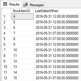
Shown above are the IDs for each updated row as well as the time it was last updated BEFORE this statement was executed. The ability to access both the INSERTED and DELETED tables simultaneously when updating data can save time and T-SQL. As with triggers, a DELETE statement can only meaningfully access the DELETED table, whereas an INSERT should only use the INSERTED table.

Consider the alternative for a moment:

CREATE TABLE #StockItemIDList
        (StockItemID INT NOT NULL PRIMARY KEY CLUSTERED);
DECLARE @LastEditedWhen DATETIME2(7) = GETUTCDATE();
UPDATE StockItemHoldings
        SET BinLocation = 'Q-1',
                LastEditedWhen = @LastEditedWhen
FROM warehouse.StockItemHoldings
WHERE BinLocation = 'L-3';
INSERT INTO #StockItemIDList
        (StockItemID)
SELECT
        StockItemID
FROM warehouse.StockItemHoldings
WHERE BinLocation = 'Q-1';
-- Or alternatively WHERE LastEditedWhen = @LastEditedWhen

It’s a bit longer and requires double-dipping into the StockItemHoldings table to both update data and then retrieve information about it after-the-fact.

OUTPUT provides convenience and allows data to be modified while simultaneously collecting details about those modifications. This can save time, resources, and allow for simpler code that is easier to read and maintain. It may not always be the best solution but can provide added utility and simplified code when no other alternative exists that is as clean as this one.

Some useful dynamic management views

Books could easily be written on how to use dynamic management views for fun and profit, so I’ll stick to a handful that are simple, easy to use, and contain information that would otherwise be a hassle to get within SQL Server:

SELECT * FROM sys.dm_os_windows_info
SELECT * FROM sys.dm_os_host_info
SELECT * FROM sys.dm_os_sys_info

These provide some basic details about Windows and the host that this SQL Server runs on:

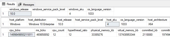
If you need to answer some quick questions about the Windows host or its usage, these are great views to interrogate for answers. This one provides details about SQL Server Services:

SELECT * FROM sys.dm_server_services

Included are SQL Server, SQL Server Agent, as well as any others that are controlled directly by SQL Server (such as full-text indexing):

More useful info that is more convenient to gather via a query than by manually visiting using a UI. This is particularly valuable data as any one of these columns could otherwise be a hassle to get across many servers. The service account can be used to answer audit questions or validate that those services are configured correctly. Likewise, the last startup time is helpful to understanding uptime, maintenance, or unexpected restarts.

This DMV lists the registry settings for this SQL Server instance:

SELECT * FROM sys.dm_server_registry

The results can be lengthy, but being able to quickly collect and analyze this data can be a huge time-saver when researching server configuration settings:

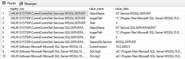
The alternatives of using the UI or some additional scripting to read these values are a hassle, and this dynamic management view provides a big convenience bonus! Note that only registry entries associated with the SQL Server instance are documented here. This includes port numbers, execution parameters, and network configuration details.

One final view that also provides some OS-level details that are otherwise a nuisance to get:

SELECT
        master_files.name,
        master_files.type_desc,
        master_files.physical_name,
        master_files.size,
        master_files.max_size,
        master_files.growth,
        dm_os_volume_stats.volume_mount_point,
        dm_os_volume_stats.total_bytes,
        dm_os_volume_stats.available_bytes
FROM sys.master_files
CROSS APPLY sys.dm_os_volume_stats(master_files.database_id,
         master_files.file_id);

Dm_os_volume_stats returns information about volume mount points, their total/available space, and lots more:

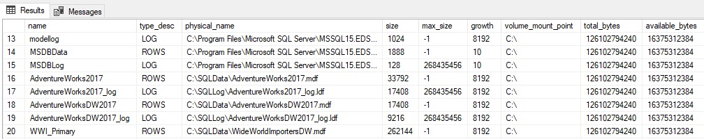
The results are a great way to check the size and growth settings for each file for databases on this SQL Server, as well as overall volume mount point details. There are many more columns available in these views that may prove useful, depending on what details are needed. Feel free to SELECT * from these views to get a better idea of their contents.

Getting results using less T-SQL

The best summary for this discussion is that there are often many ways to solve a problem in SQL Server. Ultimately, some of those methods will be faster, more reliable, and/or require less computing resources. When knee-deep in code, don’t hesitate to stop and look around for better ways to accomplish a complex task. It is quite possible that a new version, service pack, or even CU of SQL Server contains a function that will make your life dramatically easier (DATEFROMPARTS anyone? How about STRING_SPLIT?). Hopefully, the tips in this article make your life a bit easier – and feel free to share your personal favorites as well!

If you like this article, you might also like Efficient Solutions to Gaps and Islands Challenges

The post Getting results using less T-SQL appeared first on Simple Talk.

from Simple Talk https://ift.tt/DxnF3i0
via

Mighty Tester: Damned if you do, damned if you don’t

Commentary Competition

Enjoyed the topic? Have a relevant anecdote? Disagree with the author? Leave your two cents on this post in the comments below, and our favourite response will win a $50 Amazon gift card. The competition closes two weeks from the date of publication, and the winner will be announced in the next Simple Talk newsletter.

The post Mighty Tester: Damned if you do, damned if you don’t appeared first on Simple Talk.

from Simple Talk https://ift.tt/QP1OGfW
via

Oracle optimizer removing or coalescing subqueries

The series so far:

1. Transformations by the Oracle Optimizer
2. The effects of NULL with NOT IN on Oracle transformations
3. Oracle subquery caching and subquery pushing
4. Oracle optimizer removing or coalescing subqueries

So far, this series has examined the shape of some of the execution plans that Oracle’s optimizer can produce when there are subqueries in the WHERE clause and noted that the optimizer will often unnest a subquery to produce a join instead of using a filter operation that repeatedly runs the subquery. You’ve also seen that it’s possible to dictate the optimizer’s choice and have some control over the point in the execution plan where the filter operation takes place.

This installment moves on to a couple of the more sophisticated transformations that the optimizer can apply to reduce the number of subqueries that end up in the execution plan.

Removing aggregate subqueries

If you browse any of the public Oracle forums you’ve probably seen suggestions that certain patterns of queries would be more efficient if they were rewritten to use analytic functions rather than using a strategy involving self-referencing subqueries. It’s not commonly known that you don’t necessarily have to rewrite such queries; you may simply be able to tell the optimizer to do an internal rewrite for you.

To demonstrate this, I’ll use the emp and dept tables from the scott schema ($ORACLE_HOME/rdbms/admin/utlsampl.sql) as I did in the previous installment, running the demonstration from SQL*Plus on Oracle 19c (19.11.0.0). I’m going to both extend and simplify the query I wrote in that installment for ‘employess with a salary greater than the departmental average.’ The extension is that I’m going to include the department name in the output; the simplification is that I’m going to remove (temporarily) the reference to nvl(comm,0):

select
        /*+
                qb_name(main)
        */
        e1.*, d.dname
from    emp e1, dept d
where   d.deptno = e1.deptno
and     e1.sal > (
                select  /*+ qb_name(subq) */
                        avg(e2.sal)
                from    emp e2
                where   e2.deptno = d.deptno
        )
order by
        e1.deptno, e1.empno
/

You might not expect the addition of the department name or the elimination of the nvl() expression to make a significant difference to the optimizer, but the resulting plan is dramatically different. Thanks to referential integrity, the dept table behaves as a sort of ‘focal point,’ allowing the optimizer to connect the two appearances of the emp table and use a mechanism to ‘remove aggregate subquery.’ Here’s the execution plan for the modified query (generated by autotrace):

----------------------------------------------------------------------------------
| Id  | Operation             | Name     | Rows  | Bytes | Cost (%CPU)| Time     |
----------------------------------------------------------------------------------
|   0 | SELECT STATEMENT      |          |    14 |  1694 |     6  (34)| 00:00:01 |
|   1 |  SORT ORDER BY        |          |    14 |  1694 |     6  (34)| 00:00:01 |
|*  2 |   VIEW                | VW_WIF_1 |    14 |  1694 |     5  (20)| 00:00:01 |
|   3 |    WINDOW SORT        |          |    14 |   756 |     5  (20)| 00:00:01 |
|*  4 |     HASH JOIN         |          |    14 |   756 |     4   (0)| 00:00:01 |
|   5 |      TABLE ACCESS FULL| DEPT     |     4 |    52 |     2   (0)| 00:00:01 |
|   6 |      TABLE ACCESS FULL| EMP      |    14 |   574 |     2   (0)| 00:00:01 |
----------------------------------------------------------------------------------
Predicate Information (identified by operation id):
---------------------------------------------------
   2 - filter("VW_COL_11" IS NOT NULL)
   4 - access("D"."DEPTNO"="E1"."DEPTNO")

The optimizer has eliminated the aggregate subquery, reducing the query from three tables and two blocks to a simple two-table join with an analytic aggregate – at least that’s what the window sort operation and the generated view name vw_wif_1 suggest.

It’s a reasonable guess that the internal rewrite uses the avg() over approach, but this is a case where you probably ought to check the 10053 (CBO) trace file if you want to be confident about the details. Here’s the ‘unparsed’ query (extracted from the trace file but with a lot of cosmetic editing) that the optimizer finally produced for costing this plan:

select  /*+ qb_name (main) */ 
   vw_wif_1.item_1 empno, vw_wif_1.item_2 ename, vw_wif_1.item_3 job,
   vw_wif_1.item_4 mgr, vw_wif_1.item_5 hiredate, vw_wif_1.item_6 sal,
   vw_wif_1.item_7 comm, vw_wif_1.item_8 deptno, vw_wif_1.item_9 dname 
from    (
   select 
        e1.empno item_1, e1.ename item_2, e1.job item_3, 
        e1.mgr item_4, e1.hiredate item_5, e1.sal item_6,
        e1.comm item_7, e1.deptno item_8, d.dname item_9,
        case
             when e1.sal > avg(e1.sal) over (partition by e1.deptno) 
             then e1.rowid 
             end  vw_col_10 
   from 
        test_user.dept d,
        test_user.emp e1 
   where
        d.deptno = e1.deptno
        ) vw_wif_1 
where 
        vw_wif_1.vw_col_10 is not null 
order by 
        vw_wif_1.item_8,
        vw_wif_1.item_1
/

It’s interesting to note that the optimizer has introduced a CASE expression in the inline view (vw_wif_1) to generate a column that can be tested for nullity in the main query block. The human version for this strategy would probably have been to generate the ‘average over department’ as a column in the inline view that could be compared with sal in the outer query, e.g.:

select
        e2.* 
from
        (
        select 
                e1.*, d.dname,
                avg(e1.sal) over(partition by e1.deptno) avg_sal
        from    emp e1, dept d
        where   d.deptno = e1.deptno
        )       e2
where
        e2.sal > e2.avg_sal
order by
        e2.deptno,
        e2.empno
/

I said I’d simplified the query by removing the reference to nvl(comm,0); I had to do this initially because the transformation would otherwise not be used. Eventually, I did get the transformation to appear with the expression sal + nvl(comm,0), but I had to add a virtual column to the table matching the expression and rewrite the query using the virtual column:

alter table emp add nvl_earnings -- invisible
        generated always as (sal + nvl(comm,0))
/

This anomaly is probably one introduced in Oracle 19.9 by a fix for bug 30593046 which produced wrong results in some cases involving ‘scalar subquery unnesting’ in 12.2.0.1. Unfortunately, the fix blocked too many cases where unnesting was safe, so a replacement bug fix (33325981) appeared in 19.13 to restore some of the blocked cases. However, my example (where unnesting is a necessary precursor to subquery removal) still isn’t allowed past the block. When I ran the test case on 12.2.0.1, the optimizer did unnest the subquery with the original expression but didn’t carry on to remove the subquery.

In previous installments, I’ve discussed using hints to control the optimizer’s strategy when you think you know more about the data than the optimizer does. In this case, the transformation relies on sorting (i.e., the Window Sort at operation 3), so there are likely to be occasions when a bad choice of plan does a lot more work than the optimizer’s arithmetic suggests, and you might want to block the transformation. Conversely there may be cases where the transformation doesn’t appear when it would be a really good idea. Unfortunately, even though the transformation has been available since 10gR2, there is no custom hint to force it or block it. The best you can do if you want to stop the transformation from taking place is to disable the feature using an alter session command or adding the opt_param() hint to the query: opt_param(‘_remove_aggregate_subquery’,’false’). However, if you think the optimizer isn’t using the transformation when it should be, there’s not a lot you can do about it. It’s possible that you may find cases where a hint to unnest the critical subquery will result in the optimizer deciding to go one step further and remove the subquery – but that’s just a conjecture, I haven’t yet produced an example to demonstrate that this is actually possible.

Coalescing subqueries

Consider the following query which will be repeated in its full context a little later:

select  /*+ qb_name(main) */
        *
from    test_t1 t1
where 
        t1.is_deleted='N' 
and     (
            t1.id2 in (select /*+ qb_name(id2) */ t2.id2 
                       from test_t2 t2 
                       where t2.is_deleted='N' and t2.id=:p_id
                       )
         or t1.id3 in (select /*+ qb_name(id3) */ t2.id2 
                       from test_t2 t2 
                       where t2.is_deleted='N' and t2.id=:p_id
                       )
        );

When you examine the two subqueries, you’ll notice that they are identical, and both are driven by the same bind variable :p_id. The same subquery appears twice because the result is compared with two different columns from table test_t1, so it’s tempting to ask the question: “can we get each row just once then compare it twice?”

Since the optimizer often converts IN subqueries into existence subqueries you could consider transforming both these subqueries into existence subqueries then merging them into a single subquery that pushes the OR condition inside the subquery, doing something like:

Step 1:

and     (
    exists (select /*+ qb_name(id2) */ null 
           from test_t2 t2 
           where t2.is_deleted='N' and t2.id=:p_id 
           and t2.id2 = t1.id2
          )
    or exists (select /*+ qb_name(id3) */ null 
               from test_t2 t2 
               where t2.is_deleted='N' and t2.id=:p_id 
                   and t2.id2 = t1.id3
                   )
        );

Step 2:

and     (
            exists (select /*+ qb_name(SEL$????????) */ null 
                    from test_t2 t2 
                    where t2.is_deleted='N' and t2.id=:p_id 
                    and (t2.id2 = t1.id2 or t2.id2 = t1.id3)
                   )
        );

The mechanism displayed in step 2 is known as ‘subquery coalescing,’ and it has been available to the optimizer and enabled since 11.2.0.1, and comes complete with the pair of hints /*+ [no_]coalesce_sq() */.

In this example, it’s, fairly obvious that if you had an index on nothing but t2(is_deleted, id) and if (despite the clue in the second column name) there were lots of rows matching the predicates t2.is_deleted=’N’ and t2.id = :p_id then it would make sense to combine the two subqueries so that you would only have to visit those rows once each, and could stop at the first occurrence of either the t1.id2 value or the t1.id3 value. On the other hand, if you had an index like t2(id, id2) there may be no benefit gained from the transformation, so it’s nice that the mechanism can be blocked with a simple hint.

In fact, someone raised a question about this specific example in one of the public Oracle forums because the transformation had had a most undesirable side effect and produced a bad plan that took far longer to run than the best possible plan. Here’s some code (supplied on the forum, but with a few enhancements) to produce a model of what the data looked like:

rem
rem     Script:         coalesce_sq_2.sql
rem     Author:         Forum Member, edited: Jonathan Lewis
rem     Dated:          March 2022
rem
create table test_t1 as
select
        level id, level id2, level id3, 'N' as is_deleted
from    dual
connect by
        level < 1e5
;
alter table test_t1 add constraint test_t1_pk primary key (id);
create index test_t1_idx2 on test_t1(id2);
create index test_t1_idx3 on test_t1(id3);
create table test_t2 as select * from test_t1;
alter table test_t2 add constraint test_t2_pk primary key (id);
variable p_id number
exec :p_id := 5000
alter session set statistics_level = all;
set serveroutput off
select  /*+ qb_name(main) */
        *
from    test_t1 t1
where 
        t1.is_deleted='N' 
and     (
            t1.id2 in (select /*+ qb_name(id2) */ t2.id2 
                       from test_t2 t2 
                       where t2.is_deleted='N' and t2.id=:p_id
                       )
         or t1.id3 in (select /*+ qb_name(id3) */ t2.id2 
                       from test_t2 t2 
                       where t2.is_deleted='N' and t2.id=:p_id
                       )
        );
select * 
from table(dbms_xplan.display_cursor(format=>' allstats last -rows'));

Here’s the resulting plan:

--------------------------------------------------------------------------------------------
| Id  | Operation                    | Name       | Starts | A-Rows |   A-Time   | Buffers |
--------------------------------------------------------------------------------------------
|   0 | SELECT STATEMENT             |            |      1 |      1 |00:00:00.24 |     200K|
|*  1 |  FILTER                      |            |      1 |      1 |00:00:00.24 |     200K|
|*  2 |   TABLE ACCESS FULL          | TEST_T1    |      1 |  99999 |00:00:00.01 |     305 |
|*  3 |   TABLE ACCESS BY INDEX ROWID| TEST_T2    |  99999 |      1 |00:00:00.17 |     200K|
|*  4 |    INDEX UNIQUE SCAN         | TEST_T2_PK |  99999 |  99999 |00:00:00.09 |     100K|
--------------------------------------------------------------------------------------------
Predicate Information (identified by operation id):
---------------------------------------------------
   1 - filter( IS NOT NULL)
   2 - filter("T1"."IS_DELETED"='N')
   3 - filter((("T2"."ID2"=:B1 OR "T2"."ID2"=:B2) AND "T2"."IS_DELETED"='N'))
   4 - access("T2"."ID"=:P_ID)

As usual, when pulling a live execution plan from memory the text of the subquery used for the FILTER at operation 1 has disappeared from the Predicate Information, but you can infer from the predicates reported at operation 3 that subquery coalescing has taken place. For confirmation, you could use explain plan and dbms_xplan.display() to get a report that shows the missing predicate information (being careful to remember that explain plan knows nothing about the bind variable – not even its type – which is why you see to_number(:p_id) in the following:

1 - filter( EXISTS (SELECT /*+ QB_NAME ("ID2") */ 0 
                       FROM "TEST_T2" "T2" WHERE
              "T2"."ID"=TO_NUMBER(:P_ID) 
              AND ("T2"."ID2"=:B1 OR "T2"."ID2"=:B2) AND
              "T2"."IS_DELETED"='N'))

In fact, if you had reported the outline information in the call to dbms_xplan.display_cursor(), you would also have seen that it included the following two directives:

Outline Data
-------------
      COALESCE_SQ(@"ID3")
      COALESCE_SQ(@"ID2")

The key thing to note, however, is the amount of work that Oracle has had to do. For every row in the table, it has executed that subquery. Looking at the definition of table test_t2 (and especially its primary key) it’s easy to see that there can be at most one row where t2.id = :p_id, so why didn’t the optimizer unnest the subquery and use it to drive into test_t1? The answer is that while you would use only one row and one value of t2.id2 to drive a join into test_t1, there are two different columns in test_t1 in the query, and you’d have to do something complicated to unravel the pieces and join to test_t1 twice per row from test_t2 – so the optimizer doesn’t (yet) try it. There are further comments about this complication in the following blog article by Mohamed Houri: https://hourim.wordpress.com/2017/08/12/unnesting-of-coalesced-subqueries/

Since subquery coalescing has blocked a strategy that seems sensible to the human eye it’s worth telling the optimizer not to use the feature just to see if something interesting happens. Add the no_coalesce_sq() hint for the two named subquery blocks to the main query:

select  /*+
                qb_name(main)
                no_coalesce_sq(@id2)
                no_coalesce_sq(@id3)
--              or_expand(@main (1) (2))
        */
        *
from    test_t1 t1
where   
               t1.is_deleted='N' 
and     (
            t1.id2 in (select /*+ qb_name(id2) */ t2.id2 
                       from test_t2 t2 
                       where t2.is_deleted='N' and t2.id=:p_id
                       )
         or t1.id3 in (select /*+ qb_name(id3) */ t2.id2 
                       from test_t2 t2 
                       where t2.is_deleted='N' and t2.id=:p_id
                       )
        );

The or_expand(@main (1) (2)) hint – that I’ve commented out here – was something I added to force 12.2.0.1 to produce the plan that I got from 19.11.0.0. Here’s the more complicated, but far more efficient, execution plan that appeared:

-----------------------------------------------------------------------------------------------------------
| Id | Operation                               | Name            | Starts | A-Rows |   A-Time   | Buffers |
-----------------------------------------------------------------------------------------------------------
|  0 | SELECT STATEMENT                        |                 |      1 |      1 |00:00:00.01 |      16 |
|  1 |  VIEW                                   | VW_ORE_7F40D524 |      1 |      1 |00:00:00.01 |      16 |
|  2 |   UNION-ALL                             |                 |      1 |      1 |00:00:00.01 |      16 |
|  3 |    NESTED LOOPS                         |                 |      1 |      1 |00:00:00.01 |       7 |
|* 4 |     TABLE ACCESS BY INDEX ROWID         | TEST_T2         |      1 |      1 |00:00:00.01 |       3 |
|* 5 |      INDEX UNIQUE SCAN                  | TEST_T2_PK      |      1 |      1 |00:00:00.01 |       2 |
|* 6 |     TABLE ACCESS BY INDEX ROWID BATCHED | TEST_T1         |      1 |      1 |00:00:00.01 |       4 |
|* 7 |      INDEX RANGE SCAN                   | TEST_T1_IDX2    |      1 |      1 |00:00:00.01 |       3 |
|* 8 |    FILTER                               |                 |      1 |      0 |00:00:00.01 |       9 |
|  9 |     NESTED LOOPS                        |                 |      1 |      1 |00:00:00.01 |       6 |
|*10 |      TABLE ACCESS BY INDEX ROWID        | TEST_T2         |      1 |      1 |00:00:00.01 |       3 |
|*11 |       INDEX UNIQUE SCAN                 | TEST_T2_PK      |      1 |      1 |00:00:00.01 |       2 |
|*12 |      TABLE ACCESS BY INDEX ROWID BATCHED| TEST_T1         |      1 |      1 |00:00:00.01 |       3 |
|*13 |       INDEX RANGE SCAN                  | TEST_T1_IDX3    |      1 |      1 |00:00:00.01 |       2 |
|*14 |     TABLE ACCESS BY INDEX ROWID         | TEST_T2         |      1 |      1 |00:00:00.01 |       3 |
|*15 |      INDEX UNIQUE SCAN                  | TEST_T2_PK      |      1 |      1 |00:00:00.01 |       2 |
-----------------------------------------------------------------------------------------------------------
Predicate Information (identified by operation id):
---------------------------------------------------
   4 - filter("T2"."IS_DELETED"='N')
   5 - access("T2"."ID"=:P_ID)
   6 - filter("T1"."IS_DELETED"='N')
   7 - access("T1"."ID2"="T2"."ID2")
   8 - filter(LNNVL( IS NOT NULL))
  10 - filter("T2"."IS_DELETED"='N')
  11 - access("T2"."ID"=:P_ID)
  12 - filter("T1"."IS_DELETED"='N')
  13 - access("T1"."ID3"="T2"."ID2")
  14 - filter(("T2"."ID2"=:B1 AND "T2"."IS_DELETED"='N'))
  15 - access("T2"."ID"=:P_ID)

A key feature that you can spot very easily is that this plan accesses a total of only 16 buffers, handling only a few rows, rather than accessing 200,000 buffers and handling 10,000 rows. It’s clearly a significant reduction in the workload, but how does this plan actually work?

Effectively the optimizer has turned the OR’ed pair of subqueries into a UNION ALL, then unnested the union all, then pushed the join to test_t1 inside the UNION ALL (in a step rather like the reverse of join factorization – which will be reviewed in a future installment). To eliminate rows that have already appeared in the first branch of the UNION ALL the optimizer has then added a filter subquery to the second branch.

You might note that if I had not had a unique (primary key) index on test_t2 there would have been SORT UNIQUE operations applied to the rows selected from test_t2 in both branches before the joins into test_t1.

In effect the query has been transformed into:

select  {columns}
from    t2, t1
where   t1.id2 = t2.id2 and etc...
union all
select  {columns}
from    t2, t1
where   t1.id3 = t2.id2 and etc...
and     not exists (
                select {columns}
                from    t2, t1
                where  t1.id2 = t2.id2
        )

I won’t extract and reformat the ‘unparsed’ query from the CBO trace file since it is a little long and messy and adds little value to the SQL sketch above. Notice, however, from the Predicate Information provided by the call to explain plan that where I’ve used not exists(subquery) in the simplified framework, the optimizer actually uses lnnvl( exists( subquery ) ) at operation 8 of the plan. Oracle is just applying its generic ‘does not evaluate to true’ function to allow for possible nulls rather than using a simple ‘not’.

Although the resulting plan looks a little complex it is just a combination of a small number of simple transformations done in the right order, so it’s a little surprising that the optimizer doesn’t find it automatically as it searches its space of transformations. This omission has now been noted as (unpublished) bug 33957043: “Subquery Coalesce prevents Or Expansion/transformation”.

As a reminder about how difficult it is to use hints to control the fine detail of the optimizer, when I checked the Outline Information for this execution plan, it held 35 hints that would be needed in an SQL Plan Baseline to reproduce the plan. Though the list included an or_expand() hint, the no_coalesce_sq() hint didn’t make an appearance.

Summary

Converting an aggregate subquery strategy to an analytic function strategy is a rewrite that many people now do by hand when they spot the option and the numbers look right. The optimizer can do this as an internal transformation, though it doesn’t seem to take the option as often as it could. Unfortunately, there’s no explicit hint to force the transformation (though an unnest() hint may have a lucky side effect), and the only possible hint to block it is the opt_param() hint which may be needed in cases where the transformation introduces a large sorting overhead. In some cases, you may need to help the optimizer to pick the path by simplifying the SQL through the use of virtual columns, but that requirement may become redundant in a future release.

If you have multiple subqueries which look sufficiently similar and are used in a similar fashion, the optimizer can do the equivalent of ‘find the least common multiple’ so that it has to run a smaller number of subqueries, potentially using each call for multiple tests. This transformation has a related pair of hints, so it can be blocked or (if legal) forced. The demonstration of the transformation in this article highlighted a case where the optimizer missed an opportunity for using or expansion after doing subquery coalescing, so it’s worth knowing that the mechanism can be blocked.

A future installment will examine Or Expansion and Join Factorisation.

The post Oracle optimizer removing or coalescing subqueries appeared first on Simple Talk.

from Simple Talk https://ift.tt/WrKtRFL
via

Memory profiling in Python with tracemalloc

Memory profiling is useful when looking at how much memory an application is using. The most important use case, however, is when you suspect that the application is leaking memory, and it is important to trace where that leak occurs in the code.

A memory leak happens when a block of memory allocated by an application is not released back to the operating system, even after the object is out of scope and there are no remaining references to it. When this happens, memory utilization keeps increasing, until an OOM (out-of-memory error) occurs, and the operating system kills the application. If the utilization metric is plotted on a graph, it will display a constantly growing trend until the application dies. If the application restarts itself after the OOM, it will exhibit a sawtooth behavior, indicating the repeated increase and sudden drop at OOM. In programming languages where the compiler/interpreter doesn’t manage allocations, a leak can occur if the developer forgets to free allocated memory. It is, however, not uncommon, to see memory leaks in memory-managed languages as well.

Python manages memory allocations itself. Python’s memory manager is responsible for all allocations and deallocations on the private heap. By default, Python uses reference counting to keep track of freeable objects. The optional garbage collector provides supplemental mechanisms to detect unreachable objects, otherwise not reclaimed due to cyclic referencing.

Several tools are available for profiling memory in Python. This article covers “tracemalloc” which is part of the standard library. Getting started is very easy because no special installation is needed. One can start profiling and viewing the statistics straight out of the box. Tracemalloc provides statistics about objects allocated by Python on the heap. It does not account for any allocations done by underlying C libraries.

The profiler works by letting you take a snapshot of memory during runtime. There are several convenient APIs to then display the statistics contained in that snapshot, grouped by filename or lineno. It is also possible to compare two snapshots, which helps identify how memory use changes over the course of program execution. Finally, there are methods to display the traceback to where a block of memory is allocated in the code.

I will go through an example that simulates constant growing memory (similar to a leak) and how to use the tracemalloc module to display statistics and eventually trace the line of code introducing that leak.

Tracing a memory leak

Here is a one-liner function called mem_leaker() that will be used to simulate the memory leak. It grows a global array by ten thousand elements every time it is invoked.

arr = []
def mem_leaker():
        '''Appends to a global array in order to simulate a memory leak.'''
        arr.append(np.ones(10000, dtype=np.int64))

I wrapped this function inside a script named memleak.py with some driver code. The first thing to do is to call tracemalloc.start() as early as possible in order to start profiling. The default frame count is 1. This value defines the depth of a trace python will capture. The value can be overridden by setting PYTHONTRACEMALLOC environment variable to a desired number. In this example, I am passing a value of “10” to set the count to ten at runtime.

The tiny for loop iterates five times, invoking the make-shift memory leaker each time. The call to gc.collect() just nudges Python’s garbage collector to release any unreachable memory blocks to filter out noise. Although, you can be sure this program does not create any cyclic references.

Listing: memleak.py

import gc
import tracemalloc

import numpy as np

import profiler

arr = []
def mem_leaker():
        '''Appends to a global array in order to simulate a memory leak.'''
        arr.append(np.ones(10000, dtype=np.int64))


if __name__ == '__main__':
        tracemalloc.start(10)

        for _ in range(5):
            mem_leaker()
            gc.collect()
            profiler.snapshot()

        profiler.display_stats()
        profiler.compare()
        profiler.print_trace()

All the profiling code is written inside a separate script called profiler.py.

Listing: profiler.py

import tracemalloc

# list to store memory snapshots
snaps = []

def snapshot():
        snaps.append(tracemalloc.take_snapshot())


def display_stats():
        stats = snaps[0].statistics('filename')
        print("\n*** top 5 stats grouped by filename ***")
        for s in stats[:5]:
            print(s)


def compare():
        first = snaps[0]
        for snapshot in snaps[1:]:
            stats = snapshot.compare_to(first, 'lineno')
            print("\n*** top 10 stats ***")
            for s in stats[:10]:
              print(s)


def print_trace():
        # pick the last saved snapshot, filter noise
        snapshot = snaps[-1].filter_traces((
            tracemalloc.Filter(False, "<frozen importlib._bootstrap>"),
            tracemalloc.Filter(False, "<frozen importlib._bootstrap_external>"),
            tracemalloc.Filter(False, "<unknown>"),
        ))
        largest = snapshot.statistics("traceback")[0]

        print(f"\n*** Trace for largest memory block - ({largest.count} blocks, {largest.size/1024} Kb) ***")
        for l in largest.traceback.format():
            print(l)

 

Going back to the for loop in the driver code, after mem_leaker() is invoked, profiler.snapshot(), which is just a wrapper around tracemalloc.take_snapshot(), will take a snapshot and store it in a list. The length of the list will be five at the end of the loop.

Once you have the snapshots, you can see how much memory was allocated. It can be useful to begin with per file grouping if the application is big, and you have no idea where the leak is happening. For demonstration, take a closer look at profiler.display_stats(); it displays the first five grouped items from the first snapshot.

def display_stats():
        stats = snaps[0].statistics('filename')
        print("\n*** top 5 stats grouped by filename ***")
        for s in stats[:5]:
            print(s)

The output looks like this.

At the top of the list, numpy’s numeric.py allocated 78.2 Kb of memory. The tracemalloc module itself will also use some memory for profiling. That should be ignored during observation.

Comparing snapshots and observing trends

Now, in order to debug further, The code compared the first snapshot with each subsequent snapshot to see the top ten differences using compare().

def compare():
        first = snaps[0]
        for snapshot in snaps[1:]:
            stats = snapshot.compare_to(first, 'lineno')
            print("\n*** top 10 stats ***")
            for s in stats[:10]:
              print(s)

The complete output of compare() looks like this.

Since there were five total snapshots, there are four sets of statistics from the comparisons. Some important observations here:

• numpy/core/numeric.py at line 204, is at the top in each set, allocating the most memory.
• Now, note the change in memory usage by numeric.py as I go over each of the result sets.

In the first set, the total memory used by numeric.py is 156 Kb, an increase of 78 Kb from the first snapshot.

In the second set, total memory used by numeric.py jumps to 235 Kb, a total increase of 156 Kb from the first snapshot. Doing a little math, this also means there was an increase of ~79 Kb since the last snapshot.

In the third set, total memory used by numeric.py jumps to 313 Kb, a total increase of 235 Kb from the first snapshot. This also means there was again an increase of ~78 Kb since the last snapshot.

In the fourth set, total memory used by numeric.py jumps to 391 Kb, a total increase of 313 Kb from the first snapshot. This also means there was, once again, an increase of ~78 Kb since the last snapshot.

• A clear cumulative trend can be seen here in the allocation done by numeric.py. At each iteration, ignoring rounding differences, ~78 Kb more memory was allocated. If you look at mem_leaker() again, it appends ten thousand elements to the array, each of size 8 bytes, which brings the total to 80000 bytes, or 78.125 Kb. This matches the observed increase from the snapshot deltas.
• It is constantly growing trends like this that eventually lead to a code problem if the growth pattern is unexpected.

See a traceback

The last thing in the example was to print the traceback for the largest memory block for more granularity. In this case, the largest block is one from numeric.py. The filter_traces() method is very helpful in eliminating noise when debugging long traces.

def print_trace():
        # pick the last saved snapshot, filter noise
        snapshot = snaps[-1].filter_traces((
            tracemalloc.Filter(False, "<frozen importlib._bootstrap>"),
            tracemalloc.Filter(False, "<frozen importlib._bootstrap_external>"),
            tracemalloc.Filter(False, "<unknown>"),
        ))
        largest = snapshot.statistics("traceback")[0]

        print(f"\n*** Trace for largest memory block - ({largest.count} blocks, {largest.size/1024} Kb) ***")
        for l in largest.traceback.format():
            print(l)

The trace looks like this.

This trace leads from the application code to the line in the numpy library, where the allocation actually takes place. You can look at the source code here – https://ift.tt/UJbdgfr.

Conclusion

Here, you saw a simple demonstration of using Python stdlib’s tracemalloc module to observe various memory related statistics, compared snapshots to see the allocation deltas and used all this information to trace back to the code using a substantial amount of memory. In large applications, it may take some time to narrow down scope and find the line of code introducing a leak. The tracemalloc module provides all the necessary APIs to do so, and it just works out of the box.

References

https://ift.tt/eKxu13M

The post Memory profiling in Python with tracemalloc appeared first on Simple Talk.

from Simple Talk https://ift.tt/p0GBTQU
via

Change Management and Leadership Alignment

The series so far:

1. What is Change Management?
2. Change Management and Leadership Alignment

One of the fundamental Change Management principles is Leadership or Stakeholder Alignment. This principle plays an important part in implementing change across an organization, as it gathers buy-in from individuals across an organization from the top down.

As you learned in the previous article of this series, change management is the strategy used to prepare, implement, and continue change within an organization. In taking a deep dive into the Leadership Alignment piece of the change management puzzle, it is important to understand that organizational change can be different for each organization. For some, it could imply a merger or acquisition, while for others, it could mean lay-offs or even pay cuts impacting the organization’s workforce. While these are more common examples of organizational change, one often overlooked is the implementation of new technology. 

C-Level executives are known for their involvement in mergers and acquisitions or workforce shake-ups, but they usually leave the technological development within their organizations to middle-management. This took a shift in the 2010s, as more and more companies realized the onset of the Digital Revolution and began to create roles for CTOs or Chief Technology Officers. Despite this welcome change, many of the change management activities needed during a technological implementation are often ignored even by some of the most forward-thinking organizations. The fundamental problem these companies often face is a lack of Leadership Alignment behind a technological shift. 

One of the first things to consider when dealing with change, is the audience impacted by the change. The first thing that comes to mind when thinking about an org structure is usually a vertical hierarchy – It is extremely important to understand the decision makers within an organization, where the impacted users sit, and the leadership teams they sit within. What is often ignored however, is the horizontal hierarchy.

This horizontal hierarchy is often where budgets, decisions, and communications are driven from. Having alignment across these different levels ensures success in a change program. All too often, there is unity of thought when it comes to implementing a change but a lack of understanding or alignment in the intricacies of what will be needed to make that change stick. Leadership alignment is key in championing the change and supporting the change management strategy that accompanies the change and how the organization will adapt – be it through communication, training, or other forms of change management support.

In addition to the horizontal-alignment mentioned above, sponsorship from executive leadership is also imperative when implementing change. Having an executive sponsor as part of a change program helps drive visibility and alignment across all levels of an organization. Common practices around executive sponsorship include communication efforts driven by executives. These communication efforts include emails, newsletters, videos, internal product launches, happy hours, or lunch-and-learns. Having an executive sponsor as the face of these initiatives shows top-down alignment on change efforts and ensures support for the change and also for the adoption strategy, which in turn builds confidence across the organization.

A change strategy establishes the importance of leadership alignment, communication, and training. These are some of the key pillars of a successful change strategy but what is more important is to address the “What’s in it for me?” 

It is important to understand what drives motivates end users, decision makers, and executive sponsors. Understanding the pain points across these different areas of an organization is critical in winning confidence and fostering adoption. 

Depending on the engagement and the change being implemented, pain points can be approached from either a bottom-up, or a top-down approach. 

Working from the bottom-up, an engagement would usually start at the level of the end user. New technology is often implemented to make an end user more efficient or productive. This impacts all levels of the hierarchy above and around the end user because the bottom line, in terms of profitability and productivity, is often tied to the success of the end user. 

Another way to look at this is the top-down approach, which analyzes a change that starts at the executive level. Much of the reasoning for the change could be the same as it would be in a bottom-up approach (budgets, productivity, efficiency), but the way it is handled differs. In this approach, the decisions are usually made at the C-level, and regardless of the type of change in question, be it a change in org structure or business processes, the impacts of the change often trickle down across the organization. It is important to check the pulse of the organization at various stages of the change to ensure that regardless of the approach, the pain points are being addressed organization-wide.

A great way to drive change across an organization is through sponsorship. Assigning sponsors across an organization, within different business units, regions, and job levels is a great way to raise awareness about change. This approach also establishes a sense of responsibility among the sponsors, who now have a vested interest in the program’s success. This network of sponsors should be engaged early and often, allowing them to be in sync with what changes are coming, and give individuals in different parts of the organization a point of contact for feedback and concerns that may arise as part of the impending change.

At the end of the day, the purpose of leadership alignment is to ensure buy-in from leaders. All the pieces mentioned in this article, be it the understanding of an org structure, identification of top-down leadership, addressing their pain points, or establishing sponsors across the organization, are the building blocks needed for buy-in. Organizational change relies on this buy-in, as change becomes easier to foster if there is an alignment across the organization.
With buy-in and leadership alignment, the very next step in the change journey is communication. Leaders and sponsors identified through this process can help develop a communication strategy. This strategy can outline the basics, including what sort of communication is sent, who is the audience, how often communication should occur, and who should send out the communication. Establishing a communication plan empowers business leaders to rally the organization behind the change, and the next article will dive deeper into the best practices in establishing a communication strategy.

 

The post Change Management and Leadership Alignment appeared first on Simple Talk.

from Simple Talk https://ift.tt/iDVdANl
via

Power BI Last Refresh Time Visualization Tool

On the article Automating table refresh in Power BI I explained many methods to automate refresh of individual objects, which could be tables or partitions.

This creates the need of good ways to visualize the last refresh date and time for each partition and table. The portal shows the refresh date/time for the entire dataset, we can’t identify on the Power BI portal the exactly date for each table last refresh.

The Tabular Editor, famous 3rd part tool to manage Power BI models, is very powerful. It implements a c# execution engine inside it, allowing us to create scripts, from small scripts to very powerful ones.

One example is the Processing Manager published on Elegant BI blog. It creates a powerful C# program to generate refresh script for a set of objects in the model.

Based on this example, I created a C# program to visualize the last refresh date/time for each partition. It’s published on Github, you can copy the LastRefresh.cs code and execute it on the Advanced Scripting window in the Tabular Editor.

 

The result is like the image below. You will be able to see the last refresh date/time for each partition. I hope this tool is useful if you are customizing the refresh of the objects. You are also invited to improve this tool.

 

Some future improvement possibilities:

• Join this tool with the Processing Manager, calling them from a single main form.
• Make these tools an independent application
• Improve the design of the form

 

 

The post Power BI Last Refresh Time Visualization Tool appeared first on Simple Talk.

from Simple Talk https://ift.tt/xHZ6fek
via

The ins and outs of joining tables in SQL Server

There are times when you need to join multiple tables to retrieve the result set needed. SQL allows for multiple tables to be included in the FROM clause along with the criteria for how to join tables. In SQL Server there are a number of different ways to join tables. In this article, I will be discussing the ins and outs of joining two tables in SQL Server using the inner and outer join operators.

The Three Parts of a Join Operations

When two tables are joined using a join operation, the records of the two sets are logically separated into three different buckets. Those different buckets can be represented using a Venn diagram like the one in Figure 1.

Figure 1: Three parts of the JOIN Operation

Each section of the Venn diagram is represented by a different color: yellow, brown, and blue. The members of Set A that don’t match with SET B will be contained in the yellow bucket. Members of SET A and B that match end up in the brown bucket. Lastly, the members in the blue bucket are those members in SET B that don’t match with SET A. The Venn diagram can visually represent the resulting sets created when an inner or outer join operation is performed.

Test Data

To demonstrate how the different inner and outer join operations work, the examples use two test data tables created in the tempdb database. These two tables are SetA and SetB. If you want to follow along and execute the examples in this article, you can create the two test tables using the code in Listing 1.

Listing 1: Creating SetA and SetB

USE tempdb;
GO
CREATE TABLE SetA (Col1 tinyint, Col2 char(1));
INSERT INTO SetA VALUES 
        (1, 'A'), (2, 'B');
CREATE TABLE SetB (ColA tinyint, ColB char(1), ColC char(1));
INSERT INTO SetB VALUES
        (1, 'A', 'B'), (2, 'C', 'D'), (3, 'E', 'F');
GO

The two tables created when Listing 1 is run can be represented by the Venn diagram in Figure 2.

Figure 2: Tables SetA and SetB

Table SetA consists of a set with two columns (Col1 and Col2) and two different rows. Table SetB has three columns (ColA, ColB, and ColC) and contains three different rows.

INNER JOIN operator

The INNER JOIN operator is probably the most used join operation found in T-SQL code. This operator returns rows that match when two sets are joined based on one or more search criteria. The brown section in Figure 3 represents the result set of an INNER JOIN operation between the two test data tables, SetA and SetB, based on the search criterion SetA.Col2 = SetB.ColB.

Figure 3: Venn Diagram representing an INNER JOIN

The T-SQL code in Listing 2 demonstrates one way to write an INNER JOIN operation to return the matching rows found in the brown section of the Venn diagram in Figure 3.

Listing 2: Performing INNER JOIN operation

USE tempdb;
GO
SELECT * FROM SetA INNER JOIN SetB
ON SetA.Col2 = SetB.ColB;
GO

Report 1 shows the results when the code in Listing 2 is executed.

Report 1: Output produced when Listing 2 is run

The code in Listing 2 identifies the two tables, SetA and SetB, to be joined in the FROM clause, with the INNER JOIN operator between them, followed by an ON clause. The ON clause identifies the search criteria to be used when joining the two tables. In Listing 2, the ON clause specifies SetA.Col2 = SetB.ColB as the search criterion. This criterion specifies that the INNER JOIN operation is to find all the rows in SetA that have corresponding matching rows in SetB, where Col2 in SetA is equal to ColB in SetB. Let’s walk through how this join operation works.

While the technical details of how the engine joins the tables together are beyond the scope of this article, logically, SQL Server has to compare each row in SetA with each row in SetB to determine which rows match the join condition. To perform this comparison, SQL Server first finds the value for Col2 in the first row of SetA, which has a value of A. Next SQL Server scans the rows in SetB to determine if any ColB values match the value of A. SQL Server only finds a single row in SetB with a value of A in ColB. SQL server then repeats this compare process between SetA and SetB for each row in SetA, trying to find matches. The second row in SetA doesn’t match with any rows in SetB. Once all the comparisons between SetA and SetB are completed, the column values from matching rows between SetA and SetB are merged, and the final results of the INNER JOIN are returned to the calling program.

The matching search criterion used in Listing 2 uses SQL-92 join syntax. This is not the only join syntax supported by SQL Server.

Comparing join syntax between versions of SQL

In the early days of SQL, the various database vendors started implementing SQL code differently. This led to inconsistencies in how SQL code was written. In the 1980s, the American National Standards Institute (ANSI) started working on a SQL language standard. Over time the SQL standards changed the way joins could be written.

The code in Listing 2 above uses SQL-92 join syntax, which requires a join operator to be specified between the joined sets and an ON clause to identify the join criteria. Prior to SQL-92, a different syntax for joining data was used which is shown in Listing 3.

Listing 3: Performing INNER JOIN using SQL-86 join syntax

USE tempdb;
GO 
SELECT * FROM SetA, SetB
WHERE SetA.Col2 = SetB.ColB;
GO

The pre-SQL-92 syntax required a comma to be placed between tables being joined and required the join criteria be specified in the WHERE clause. By moving the join conditions to the ON clause, the SQL-92 standards separated the join conditions from other search conditions a query might have in the WHERE clause. SQL Server still supports the older method of doing the INNER JOIN operation using pre-SQL-92 syntax, but it no longer supports the outer join method using the pre-SQL-92 syntax. SQL-92 standard is now the recommended standard for doing join operations. For the rest of the join examples in this article, only the ANSI SQL-92 syntax will be shown.

The INNER JOIN operation returns rows with matching members in both the left and right sides of joined sets. However, there are times when rows might need to be included in result sets even when they don’t match. This is where the outer join operations can help.

LEFT OUTER JOIN

The LEFT OUTER JOIN operation returns all the rows from the table on the left, even when they don’t match any of the rows on the right based on the search criteria. The Venn diagram in Figure 4 logically shows the results of a LEFT OUTER JOIN operation between SetA and SetB based the search criterion of SetA.Col2 = SetB.ColB.

Figure 4: Venn diagram representing LEFT OUTER JOIN

By comparing Figure 4 to the Venn diagram for the INNER JOIN found in Figure 3, the matched row of SetA, in the brown section, and the unmatched members in the yellow section of SetA have been combined into a single yellow circle. The members of this yellow circle are the members of SetA and SetB that will be returned from the LEFT OUTER JOIN operations. Listing 4 contains the T-SQL code to produce the LEFT OUTER JOIN results represented by Figure 4.

Listing 4: LEFT OUTER JOIN

USE tempdb;
GO 
SELECT * FROM SetA LEFT OUTER JOIN SetB
ON SetA.Col2 = SetB.ColB;
GO

Report 2 shows the output when Listing 4 is executed.

Report 2: Output from running Listing 4

The results in Report 2 have one row that matched the search criterium and one that didn’t match. The row that didn’t match the column values for the table on the right side of the LEFT OUTER JOIN operation is set to NULL. It is easy to identify those rows that did not match the search criterium by checking to see if any of the columns from the right table is null, as done in Listing 5.

Listing 5: Finding rows on the left that don’t match rows on the right

USE tempdb;
GO 
SELECT * FROM SetA LEFT OUTER JOIN SetB
ON SetA.Col2 = SetB.ColB
WHERE SetB.ColA is null;
GO

When the code in Listing 5 is run, only the last row in Report 2 will be returned.

RIGHT OUTER JOIN

The RIGHT OUTER JOIN operation is similar to the LEFT OUTER JOIN operation. The difference is that all the rows in the right table are returned, whether or not they match the rows in the left table. To show this consider the code in Listing 6.

Listing 6: Right outer join example

USE tempdb;
GO 
SELECT * FROM SetA 
RIGHT OUTER JOIN SetB
ON SetA.Col2 = SetB.ColB;
GO

Report 3 shows the results when Listing 6 is executed.

Report 3: Results when Listing 6 is run

Report 3 shows that all the rows from the right table, SetB, are returned. For those rows in SetB that don’t match SetA, the NULL value was returned for the SetA columns in the result set.

If you need to find all the rows in SetB that don’t match the search criterion of SetA.Col2 = SetB.ColB, then the code in Listing 7 can be run.

Listing 7: Finding rows in SetB that don’t match SetA

USE tempdb;
GO 
SELECT * FROM SetA 
RIGHT OUTER JOIN SetB
ON SetA.Col2 = SetB.ColB
WHERE SetA.Col1 is null;
GO

Report 4 shows the results produced when Listing 7 is executed.

Report 4: Results from running Listing 7

FULL OUTER JOIN

The FULL OUTER JOIN operation combines both the LEFT and RIGHT OUTER JOIN and the INNER JOIN in a single operation. Listing 8 uses the FULL OUTER JOIN operator to find all the rows that match and don’t match the search criterion SetA.Col2 = SetB.ColB.

Listing 8: Finding all matching and unmatched rows

USE tempdb;
GO 
SELECT * FROM SetA FULL OUTER JOIN SetB
ON SetA.Col2 = SetB.ColB;
GO

Report 5 shows the results when Listing 7 is run.

Report 5: Output from Listing 8

The first row in Report 5 is the only row that meets the search criterion identified in Listing 8, hence why each column has a value. The second row is the left row that doesn’t match any rows on the right; it could be found using the LEFT OUTER JOIN. The third and fourth rows are the rows from the right that don’t match the rows from the left; they could be found using a RIGHT OUTER JOIN operation.

The code in Listing 9 shows how to find only those rows in either the left or right table that don’t match the search criterion.

Listing 9: Using the FULL OUTER JOIN

USE tempdb;
GO 
SELECT * FROM SetA FULL OUTER JOIN SetB
ON SetA.Col2 = SetB.ColB
WHERE SetA.Col1 is null or SetB.ColA is null;
GO

Report 6 shows the output when Listing 9 is executed.

Report 6: Output when Listing 9 is run

The rows from the left table that don’t match rows in the right table will have nulls in the columns from the right table. Inversely, rows from the right table that don’t match rows in the left table will have nulls identified for all the columns from the left table.

Using Multiple comparison operations

The comparison between two sets in a join operation can also have multiple comparison operations, like the code in Listing 10.

Listing 10: Using multiple comparison operators in a join operation

USE tempdb;
GO
SELECT * FROM SetA INNER JOIN SetB 
ON SetA.Col1 = SetB.ColA AND SetA.Col2 = SetB.ColB;
GO

When Listing 10 is executed the results in Report 7 is produced.

Report 7: Output when Listing 10 is run

In Listing 10 only the rows where both Col1 from Set1 matches ColA from SetB and Col2 from SetA matches ColB from SetB.

The Ins and Outs of Joining tables

Joining tables is a key skill every T-SQL programmer needs to master. In this article, I used Venn diagrams and T-SQL code examples to show on how the INNER JOIN, LEFT OUTER JOIN, RIGHT OUTER JOIN and FULL OUTER JOIN operations can be used to find different sets of records when joining two sets. Hopefully, next time you need to find the rows in one of the three parts produced when joining two sets you will know which join operation and search criteria to use.

 

The post The ins and outs of joining tables in SQL Server appeared first on Simple Talk.

from Simple Talk https://ift.tt/tRLn5yI
via

SQL Server vulnerabilities and assessment

Even with security measures in place, SQL Servers can fall prey to cyberattacks. The threat actors target the servers to gain access to the sensitive data locked away in the SQL databases as well as the backup files. As per a report by Cyber Security Experts, “Personal data of nearly 4 million individual filers and 700,000 businesses in the South Carolina Department of Revenue (DoR) was breached in August 2012. The attacker found worthy loot in the form of DoR database backup and copied the 74 GB database.” The department’s major focus was on investing in antivirus technology aimed to block an initial attack. When this line of protection was breached, they became defenseless against such attacks. However, if the organization had invested in security protection measures such as backup encryption, it could have prevented such data breaches.

Even with security measures in place, it is not an easy task to protect the SQL databases as the attackers primarily look for vulnerabilities to target the databases. Therefore, it is pertinent for database administrators (DBAs) to keep an eye on the vulnerabilities in order to protect the SQL databases from being attacked and compromised. DBAs also need to make sure that databases in downstream environments, such as dev and QA are protected, if they contain sensitive information. Redgate’s Provision can help you quickly deliver masked database to these environments. 

In this article, we’ll be mentioning some common vulnerabilities in SQL Server. Also, we’ll discuss how to assess your SQL Server for potential vulnerabilities and perform a speedy recovery of databases if compromised.

Some common vulnerabilities in SQL Database

Following are some common vulnerabilities you need to be vigilant about to protect your SQL database from being attacked.

SQL Injection

SQL Injection, also referred to as SQLi, attacks allow hackers to manipulate SQL (Structured Query Language) queries to exploit vulnerable databases. Essentially, SQLi allows threat actors to send unauthorized data to a web application, connected to databases, as part of a query or command. Executing the query or commands enables attackers to gain access or make changes to the sensitive data stored in SQL databases.

In a nutshell, SQL Injection attacks occur due to improper security encoding (or input validations) in the application or web form. As user-applied input is the contributing factor behind the SQLi attacks, controlling and inspecting user input for attack patterns can help prevent such attacks. Also, configuring a web application firewall (WAF) can help identify SQL injection attacks. Note that this is important for any SQL database, not just SQL Server.

If you use SQL Monitor, this article explains how to capture SQLi attempts.

Human errors

As per the 2021 Verizon Data Breach Investigations Report (DBIR), human errors account for 85 percent of all data breaches. Unintended actions or lack of action by an organization’s employees and users may lead to security breaches. For instance, failing to use a strong password, not installing critical software security updates, and downloading a virus-infected attachment are some human errors that contribute to accidental database breaches.

Reducing instances of human errors and educating stakeholders on security basics and best practices help them in making better, informed decisions.

Weak passwords

Weak passwords are the most common contributor of database security breaches. According to a report published by the cybersecurity division of the Chinese company Tencent, “Thousands of Microsoft SQL Servers (MSSQL) exposed to the Internet were infected with the malware gang MrbMiner that used brute-force attacks to gain access to administrator accounts that are configured with weak passwords.” Therefore, it is crucial for organizations running SQL databases on the cloud or any network to use strong passwords to combat brute-force attacks.

Extensive user privileges and installation

Although SQL Server is a highly secure database platform, certain factors like installing all the SQL database components, assigning too many permissions and roles, using multiple AD groups, etc., can leave security gaps in the system and make databases vulnerable to attacks.

You must keep these considerations in mind:

• Limit installation to only the components required by a database to perform its tasks.
• Use a least privileged service account to prevent exposing your database to security attacks.
• Connect to SQL Server using Integrated Security (i.e., Windows Authentication).
• Use encryption features available in SQL Server to keep the data (mdf) and log (ldf) files secure against unauthorized access. The features include Transparent Data Encryption (TDE), Always encrypted, etc.
• Mask sensitive databases in downstream environments like development and QA.
• Disable the SA login account in SQL Server as every database administrator and hacker knows about it.

No encryption or poor encryption

If your database or data within the database is not encrypted, the hackers can track the points of interconnection between the network and the machine to compromise the database. So, to avoid such instances, it is important that DBAs keep the SQL database or the data within the database in encrypted form. It is applicable for both the primary database and the backup files.

Missing security updates and patches

Malware attacks remain a persistent threat for databases that are missing security patches or running on older versions of SQL Server. If DBAs forget to keep the SQL Server up-to-date with the latest security patches, then the server becomes vulnerable to malware attacks.

Weak audit trail

An audit trail helps organizations track and log events performed on a server level or database level. The audit trails can be analyzed for any possible security policy violations. Also, they can aid in forensic analysis in the event of a security breach. However, organizations having weak (or non-existent) audit records may fail to determine application errors or fraudulent practices, making the databases vulnerable to attacks.

Maintaining a strong audit trail in SQL Server can help your organization run smoothly and securely. But before audit trail implementation, try understanding SQL Server Security Audit Basics.

Denial of service attack (DoS)

DoS is a security threat that cybercriminals use to shut down a system or network, preventing users from accessing the SQL database and its data. DoS can be achieved by exploiting vulnerabilities to crash a database server and flood the machine with requests or malware that obstruct the database server from providing data to the intended users.

One of the biggest examples of DoS attacks is SQL Slammer. It is a 2003 computer worm that caused denial-of-service attacks and exploited a buffer overflow vulnerability in Microsoft’s SQL Server. After a decade of no activity, the SQL Slammer worm became one of the most prevalent attacks between November 28 and December 4, 2016, that infected unpatched SQL Server version 2000.

Reviewing the use of firewalls, upgrading your SQL Server versions, and applying security patches are some of the actions you can take to protect your databases against DoS attacks (like SQL Slammer).

How to assess SQL Server for potential vulnerabilities

For SQL administrators, it is crucial to incessantly check the databases for any potential vulnerabilities to improve database security. For a long time, DBAs had to use external tools or write customized scripts to determine, track, and remediate these vulnerabilities. Fortunately, SQL Server introduced a built-in solution, the Microsoft SQL vulnerability assessment (VA) tool.

This tool helps scan the database to discover, monitor, and address security issues in your environment. It uses a knowledge base of rules warning about deviations from Microsoft’s recommended best practices, such as unprotected sensitive data, granting excessive permissions, and misconfigurations. It highlights security issues that pose the biggest threats to your database and its valuable data.

You can run the VA tool in SQL Server Management Studio (SSMS) or manage it using PowerShell cmdlets. You run VA by right-clicking on the database you want to scan and then clicking on Tasks > Vulnerability Assessment > Scan For Vulnerabilities.

Figure 1 – Running SQL Vulnerability Assessment

After completion of the scan, a scan report (see the below image) is displayed, presenting issues detected in the database and their respective severities – High, Medium, and Low. It also suggests actionable remediation information to solve the issues.

Figure 2 – Vulnerability Assessment Results for SQL Database

(Source: https://docs.microsoft.com/en-us/sql/relational-databases/security/media/sql-vulnerability-assessment/3-ssmsscanresults.png?view=sql-server-ver15)

You can drill down each on failed security check displayed in the scan report to understand the reason behind the failure. Subsequently, you can use the actionable steps suggested in the report to resolve the issue.

Figure 3 – Failed Security Checks & Remediation Action

(Source: https://docs.microsoft.com/en-us/sql/relational-databases/security/media/sql-vulnerability-assessment/3-ssmsscanresults.png?view=sql-server-ver15)

How to test backups and restore the database

If your SQL database is compromised or attacked by threat actors and becomes inaccessible, backups can help restore the database to a point in time within the retention period.

But are you certain that the backups can be restored successfully?

A recent study shows that “58 percent of backups fail, leaving data irrecoverable in the event of an outage due to cyberattack”. Besides this, other factors like a damaged tape drive or disk drive may also prevent you from restoring the backup. This is why it is crucial to test backups frequently to ensure they are error-free and restorable.

Backup verification for database backup testing

There are several built-in backup verification methods available in SQL Server to test if the backups are valid and can be used to restore the database. Let’s discuss the two backup verification methods:

1. CHECKSUM

Create backups with CHECKSUM to check the integrity of the data in the backup (see the below example).

BACKUP DATABASE [DBName]
TO  DISK = N'G:\DatabaseBackups\DBName.bak'
WITH CHECKSUM;

When used in the backup command, CHECKSUM tests the page checksums on the data pages being backed up. The backup operation stops if a bad checksum is found and returns a message identifying the bad page.

2. RESTORE VERIFYONLY

Another option is to use RESTORE VERIFYONLY to ensure whether a backup file is valid or not. This option helps validate that what was written to the backup file matches the CHECKSUM.

RESTORE VERIFYONLY
FROM DISK = N'G:\DatabaseBackups\DBName.bak';

Both RESTORE VERIFYONLY and CHECKSUM options are available in SSMS as “Verify backup when finished” and “Perform checksum before writing to media”, respectively. The options help validate that the database backup is complete and can be restored when needed. However, RESTORE VERIFYONLY does not verify the structure of the data.

Figure 4 – Reliability features of back up

Use these options when scheduling to test backups automatically.

Database restore drills

The best way to know if your backups are good or not is to perform a regular database restoration drill. The drill requires performing two steps. The first step is to restore the database from regular backups, and the second step is to run consistency checks on the restored database. You can write a T-SQL script or create an SSIS package to restore the backups and perform consistency checks.

A better alternative is to use DBATools, an open-source PowerShell module that provides several commands to perform administrative tasks in SQL Server. The command Test-DbaLastBackup helps test the most recent full database backups. It identifies the last set of full backups and transaction logs and restores all the files. Once the backup is restored, a CHECKTABLE is applied to check the integrity of database objects. All of can be accomplished this using a single Test-DbaLastBackup PowerShell command.

See SQL Backup from Redgate for a high-speed database backup, verify, and restore tool. This tool helps automatically restore and validate the backups. It also helps keep database backups protected with 256-bit AES encryption.

Use high availability (HA) and disaster recovery (DR) solutions

Use the HA and DR solutions like Log Shipping, Database Mirroring, SQL Server Always On Availability Groups, etc., to perform database recovery. These solutions help maintain copies of the SQL Server databases at multiple locations. If any unforeseen event occurs, data availability can be obtained as a secondary replica takes over the primary database.

See SQL Server High Availability and Disaster Recovery Plan for detailed information about HA and DR options.

Conclusion

This article covered how organizations that rely upon Microsoft SQL Server for deploying databases as the major data stores are vulnerable to attacks. It also gives advice on how organizations can assess SQL Server databases for vulnerabilities and gave suggestions to resolve security issues using the built-in Microsoft SQL vulnerability assessment (VA) tool. Additionally, it recommended the way forward to test database backups and restore databases.

You can test backups using the backup verification methods: RESTORE VERIFYONLY and CHECKSUM. To restore the backup, you can use the Test-DbaLastBackup PowerShell command from DBATools. If you write your own script, you can use a SQL Agent job. Another alternative is Redgate’s SQL Backup. As a last resort, failover to a secondary database if the primary database is inaccessible.

Remember, what happened once can happen again. So, it’s important to keep your database and server safe. Here’s a series on SQL Server Security you can explore to protect and secure your SQL databases.

References Used:

A Review of Critical Security Challenges in SQL-based and NoSQL Systems from 2010 to 2019

Vulnerability assessment for SQL Server

Reducing Recovery Time When Restoring a Database

 

The post SQL Server vulnerabilities and assessment appeared first on Simple Talk.

from Simple Talk https://ift.tt/uHLSvA7
via