The Job of a Technical Editor (as Louis sees it)

One of the most essential parts of producing a great technical article, blog, or even a book, (referred to from now on generally as a work) is having someone who can check your writing and make sure it is right. You can do a mediocre job with grammar, punctuation, etc. and still produce technical resources that people can get value out of. But when technical details are wrong…it is actually possible that a reader becomes less knowledgeable by reading what was supposed to be a technical resource.

In this blog, I want to put out a few guidelines that I use when am a technical editor for some piece of writing… sometimes even my own. Usually this kind of task will be done on non-academic work, sometimes called trade publications. There will be very  little new ideas put forth in the writing and the usual point is to take what can be a complex topic and simplify it for the reader. As such, it is not atypical that the writer is actually less knowledgeable about parts of the topic than desired. I know in the first version of my Database Design book (on version 6 now), I did a reasonably bad job of understanding some topics (both before and after the tech edit phase). The book overall was pretty good, with the help of some really good tech editing, but even today I have had a comment or two from academics on how my book doesn’t quite get it.

Let me clarify one point a little before proceeding with a few guidelines. I did say “even my own.” When I write a blog, I don’t have a tech editor, so I have to put a little space between myself and the writing and read the material a few times and say “is that really right?” Usually I am (and usually most writers I have worked with were too,) but usually isn’t the target. If I can’t say 100% in my mind that something is right, I still look it up.

The general process of doing a technical edit for a computer book, for me has been this:

• Scan the document, to get an idea of structure
• Read the material with a suspicious eye, like you think the author of the writing is dumber than toast. It is easier to do when it is your own work, admittedly.
• Execute every piece of code, build every VM, set up everything that is described (To your limits)
• Comment (usually in a Word document) on everything that doesn’t work
• Comment everywhere you disagree technically
• Give ideas on how to make the piece of work better
• Give feedback on how things are good

It can be a daunting task and not everyone wants a tremendous amount of feedback. Ok, no one WANTS a lot of feedback, but I know I personally am more afraid of 0 comments than I am of 100s. The following are tips I suggest people consider when they are tech editing, as much as possible:

———

Be nice – I want to start here because this can be the hardest thing. But I have heard many times from an author “thank you for the nice comment”, usually because I was tearing up the rest of the work. If you have major concerns, pointing out what is working is a great idea. (Ideally not in one of those “yeah, this is great, but actually it is not” sort of ways. Fake niceness is, to me, worse than just getting told I am doing a bad job.

Be nitpicky – The whole job is really just being nitpicky. Like really nitcpicky. (Comment: not how nitpicky is spelled) (Comment: Good point, but while being annoyingly nitpicky is a lot of the job, it really isn’t all of it. Should probably be “Most of the job…”) (Comment: check with your author/book publisher to see how nitpicky. Sometimes the target audience is important to the level being targeted. Still, right is right and wrong is never right.)

No seriously, niceness is important – Because all that nitpickiness really builds up. Most technical authors probably have experienced some serious anger/anxiety/etc from a bunch of tech edits. When you finish working on a piece of work after a tech edit it is a great feeling, and usually I look back and say “That was great! Thank you tech editor”.

Along these lines, I would generally say not to be repetitive. If the writer says something wrong repeatedly, after a few times, maybe just note that it is repeated if it is clear enough along. Not only does it start to hurt, but it gets in the way of finding other stuff.

I like it when people are verbose and offer suggestions – Say I wrote “the sky is blue”. A comment might be, “not clear, explain.” Or it could be “This isn’t clear because I am not sure when you meant. What if you said ‘The sky is blue during clear skies because of… ‘ and then explained.” When the project is nearing the end, if the comment is unclear, it is probably ignored and you probably had a good point.

Suggestions may or may not be welcomed by an author. Don’t take it bad if you are involved in a second tech edit to see comments like “this is my book, that is not what I am doing”. You may not be the tech editor for that author in the future :). 

I feel like this is part of the value you provide as a tech editor if it is desired by your author. I like nothing more than to get back a chapter with lots of suggestions as to how to be more clear, or more right. Not everyone agrees and what makes your job “good enough” is a complex topic!

Make sure you KNOW you are right or make sure to note it as such – When you are going to tell the writer that their work is wrong, make sure you can back it up. When editing something I don’t really understand, I do searches for keywords found on the web. If I don’t see it in a few places so I am sure something is wrong,  I tend to say “I think this may be wrong based on ‘sentence from a document’ linked here: https://somewhere” or sometimes just from my memory (which I will also note!) Obviously a great technical document can be backed up with lots of external documentation, most of which you won’t be linking to or citing (unless this is actually a new idea and proof of that idea… which is not typically what I am talking about here.)

Make (at least) two passes through a document –  Start out skimming the work as much as is reasonable, looking for the topics covered. As the technical author, you might suggest that things are out of order, but the worst feeling is spending 10 minutes explaining how something needs to be said, only to find it a few pages later. Done this many times. Many.

Be as thorough as expected, but not too much more – It is not your work, and your name will probably just be a brief footnote in the book, but I try to think “if it was me, what would I want”. Nothing makes me more unhappy than to find glaring errors in a piece of work that supposedly was checked over. I don’t expect perfection, and I definitely don’t deliver it, but if I have written 10-1=0, I hope that is caught even in a casual read.

(My theory on how I miss such simple stuff in my initial submissions is that as an author I have read and modified parts of the material 5-20 times and I get blind to parts of the document. Seriously start to hate every word you have written until you can be away from it for a few weeks. When you are tech editing, you generally only want to make two passes and not get that connected to the work…though that is not always possible.) 

If something smells funny, check it out – Authors at times forget the lessons of high school English: “You have to write your own material.” In the real world the rule is more “You need to produce original material.”

Sometimes it can be a ghost writer situation (having someone else write for you may or may not be allowed) that causes it to seem like 2 people wrote something. But when this is the case, it is essential that the publisher is okay with multiple authors.

The other thing to look out for is plagiarism. Even if the publisher allowed for multiple people working on the work, the other writers need to have authorized the usage. Copying and pasting from random websites is often caught by pasting sections of text into a search engine.

On more than one occasion I have searched for a sentence to find large amounts of material from a vendor’s documentation repeated exactly in the text. Best case it was unintended. Worst case it gets through and the original work’s author sues the author (and probably only the author…read your writer’s contract, they make that clear!)

Don’t change the source material unless authorized – When I do my own tech editing, I change the text as I find issues. I really don’t like changing other people’s work, and I don’t like mine changed either (unless it is a work for hire and the person paying me makes the changes…It is essentially theirs anyhow. Posting suggested changes into comments puts the onus on the writer to agree without looking through change tracking.

NEVER change a document without change tracking/commenting – Even if authorized to make changes, even if you are the technical editor for the book/website, even if it is the simplest of things. Make sure the original author can see what changes have been made.

——-

This is just a few notes on what I like to do as a technical editor, I might add to them later, but the gist of it is this. If you are technical editing a piece of work, your job is to improve the technical correctness of the work some amount. This may just be a quick overview of the work, and it could be a line by line correction of every little issue.

Discuss how deep to check correctness with the people you are working with, possibly the author or book’s editor before you do too much or too little. I personally prefer to almost prove that everything stated in the work is correct if I can, but that may not be what you are requested to do.

The post The Job of a Technical Editor (as Louis sees it) appeared first on Simple Talk.

from Simple Talk https://ift.tt/eau2CBZ
via

Summarizing data using GROUP BY and HAVING clauses

SQL Server provides the GROUP BY clause as a means to take a set of detailed values and summarize them into aggregated values. The detailed records can be aggregated based on one column, as well as expressions, which are specified in the GROUP BY clause. This article explores how to return summarized data using the GROUP BY and HAVING clauses.

Test data

In order to demonstrate how to use the GROUP BY and HAVING clauses, some test data will be needed. All of the examples in this article will use a table called Invoice that is created in tempdb, using the code in Listing 1.

Listing 1: Code to create test data

USE tempdb;
GO
CREATE TABLE Invoice (
InvoiceID INT,
InvDT DATE,
InvAmt DECIMAL(10,2),
PaymentDT Date, 
PaymentAmt DECIMAL(10,2),
ProductName VARCHAR(20)
)
GO
INSERT INTO Invoice VALUES
(1,'2021-02-14',121.11,'2021-03-01',121.11,'Thingamajig'),
(2,'2021-02-14',159.16,'2021-03-13',159.16,'Watchamacallit'),
(3,'2021-02-14',75.59,'2021-03-03',75.16,'Dohicky'),
(4,'2021-02-14',121.11,'2021-03-01',121.11,'Thingamajig'),
(5,'2021-02-14',75.59,'2021-02-21',75.16,'Dohicky'),
(6,'2021-03-03',159.16,Null,null,'Watchamacallit'),
(7,'2021-03-11',75.59,'2021-03-30',75.16,'Dohicky'),
(8,'2021-02-14',121.11,'2021-03-01',121.11,'Thingamajig'),
(9,'2021-03-11',159.16,null,null,'Watchamacallit');
GO

The code in Listing 1 created nine different invoice records in the Invoice table. Each row contains a single invoice record for one of three different ProductName’s: Thingamajig, Watchamacallit, and Dohicky. Each row has an InvDT, and an InvAmt, where the InvDT identifies the date the product was sold, and the InvAmt identifies the amount the product sold for. Each product sells for a different price, but each sale of a specific product sells for the same amount. The PaymentDT and PaymentAmt identify the date and amount each payment was made. A couple of the invoices have not been paid, hence why their PaymentDT and PaymentAmt are null.

A few different examples will be provided that use the test data in the Invoice table to demonstrate how the GROUP BY and HAVING clauses work. If you would like to run the example code provided in this article, you can use the code in Listing 1 to create the Invoice table on your instance of SQL Server.

Summarizing based on a single column

This first example shows how to write a GROUP BY clause that aggregates the rows in the Invoice table based on a single column grouping specification. This example calculates the total and average invoice amount for each product identified in the Invoice table by using the code in Listing 2.

Listing 2: Grouping based on a single column

USE tempdb;
GO
SELECT ProductName, 
SUM(InvAmt) TotalInvAmt, AVG(InvAmt) AvgInvAmt 
FROM Invoice
GROUP BY ProductName;

Report 1 shows the results when Listing 2 is executed.

Report 1: Results when Listing 2 is run

In Listing 2, the GROUP BY clause identifies only a single column named ProductName. This told SQL Server to group the rows by ProductName when calculating the TotalInvAmt and the AvgInvAmt. The TotalInvAmt for each of the different products was calculated using the SUM function, whereas the AvgInvAmt was calculated using the AVG function. Since there were only three different products sold in the Invoice table, only three summarized amounts were returned, one for each ProductName.

When a SELECT statement contains a GROUP BY clause, the columns in the select list can only be those columns identified in the GROUP BY clause, or column values calculated using an aggregate function. If there is no GROUP BY clause, then only aggregate functions can be added to the SELECT list and ORDER BY clause. In this case, the query will return one row and provide summary calculations over the entire result set. If a non-group by column is identified in the select list or ORDER BY clause, and it is not contained in an aggregate function, an error similar to the error in Report 2 will be produced.

Report 2: Error received when a column listed that is not contained in an aggregate function

Msg 8120, Level 16, State 1, Line 31

Column 'Invoice.InvDT' is invalid in the select list because it is not contained in either an aggregate function or the GROUP BY clause.

The code Listing 3 was run to generate the error in Report 2.

Listing 3: Code containing selection list column not contained in aggregate function

USE tempdb;
GO
SELECT ProductName, InvDT, 
SUM(InvAmt) TotalInvAmt, AVG(InvAmt) AvgInvAmt 
FROM Invoice
GROUP BY ProductName;

Returning a subset of summarized values

If only a subset of the summarized rows needs to be returned, then a WHERE constraint can be used to identify the subset. The code in Listing 4 uses the WHERE clause to only return the summarized values for the ProductName Dohicky.

Listing 4: Constraining result set using WHERE clause

USE tempdb;
GO
SELECT ProductName, 
SUM(InvAmt) TotalInvAmt, AVG(InvAmt) AvgInvAmt 
FROM Invoice
WHERE ProductName = 'Dohicky'
GROUP BY ProductName;

When adding the WHERE constraint to a SQL statement that contains a GROUP BY clause, the WHERE clause needs to be placed prior to the GROUP BY clause. The results shown in Report 3 are produced when the code in Listing 4 is executed.

Report 3: Output produced when Listing 4 is executed

Grouping based on multiple columns

There are times when data summarization needs to produce summarized values with more granularity than a single column. When this is needed, multiple columns can be specified in the GROUP BY criteria, as shown in Listing 5.

Listing 5: Summarizing based on ProductName and InvDT

USE tempdb;
GO
SELECT ProductName, InvDT, 
SUM(InvAmt) TotalInvAmt, AVG(InvAmt) AvgInvAmt 
FROM Invoice
GROUP BY ProductName, InvDT;

In Listing 5, two columns, ProductName and InvDT, were identified in the GROUP BY clause. This tells SQL Server to summarize the test data based on each unique combination of these two column values. Report 4 contains the output created when Listing 5 is executed.

Report 4: Output when Listing 5 is run

Sorting summarized data

You may have noticed that in the prior example, the output in Report 4 was not sorted by ProductName and InvDT, even though the data was grouped and summarized by ProductName and InvDT. The ordering of the output is based on the unique combination of the grouped columns, and not the individual values of the columns in the GROUP BY clause. The only way to guarantee the output’s order is to have an ORDER BY clause. The code in Listing 6 groups the data the same as in Listing 5, but the output is produced in a different order because an ORDER BY clause has been added in Listing 6.

Listing 6: Sorting summarized data

USE tempdb;
GO
SELECT ProductName, InvDT, 
SUM(InvAmt) TotalInvAmt, AVG(InvAmt) AvgInvAmt 
FROM Invoice
GROUP BY ProductName, InvDT
ORDER BY ProductName, InvDT;

When using the ORDER BY clause, it must be specified after the GROUP BY clause. Report 5 shows the output produced when the code in Listing 6 is executed.

Report 5: Output with Listing 6 is run

By using the ORDER BY clause, the output in Report 5 is sorted by ProductName and InvDT.

Using an expression in the GROUP BY clause

Expressions can also be used in the GROUP BY clause to identify the values to summarize on. To show how an expression can be used in the GROUP BY clause, look at the code in Listing 7.

Listing 7: Using Expression in GROUP BY clause

USE tempdb;
GO
SELECT CAST(YEAR(InvDT) as CHAR(4)) + '-' + RIGHT(MONTH(InvDT) + 100,2) YearMonth,
SUM(InvAmt) TotalInvAmt , AVG(InvAmt) AvgInvAmt
FROM Invoice
GROUP BY  CAST(YEAR(InvDT) as CHAR(4)) + '-' + RIGHT(MONTH(InvDT) + 100,2);

The code in Listing 7 summarizes the rows in the Invoice table based on the year and month of the invoice. The year and month values are calculated from the InvDT using the following expression:

CAST(YEAR(InvDT) as CHAR(4)) + ‘-‘ + RIGHT(MONTH(InvDT) + 100,2);

This expression was specified on the GROUP BY clause to identify the values for summarizing. Remember that any column specified in the selection list either needs to be used with an aggregate function or by one of the GROUP BY values. Therefore, the expression identified can be included in the selection list, so the year and month values could be displayed in the result set, as shown in Report 6.

Report 6: Output when Listing 7 is run

Grouping NULL values

When comparing two different null values by design are not equal, but when grouping on a column that contain null values, the nulls are grouped together as if they are equal. To demonstrate, run the code in Listing 8.

Listing 8: GROUP ON column with null values

USE tempdb;
GO
SELECT PaymentDT, MIN(PaymentAmt) MinPaymentAmt
FROM Invoice 
GROUP BY PaymentDT;

Report 7 shows results when Listing 8 is run.

Report 7: Output when Listing 8 is executed

There is a row in Report 7 that has NULL for PaymentDT column. This row was created when grouping together the two rows that don’t have a PaymentDT value. The value of NULL under the MinPaymentAmt column occurred because null values are ignored for all aggregate functions, except the COUNT(*) function.

Because nulls are grouped together, and most aggregate functions ignore null values, summarizing results using a GROUP BY clause might create some summarized values that some might consider inaccurate. To see how aggregate functions ignore nulls, review the rows with null values in the sample data by running the code in Listing 9.

Listing 9: Displaying sample data

USE tempdb;
GO
SELECT ProductName, PaymentAmt
FROM Invoice 
WHERE ProductName = 'Watchamacallit';

Report 8 shows the output created when Listing 9 is executed.

Report 8: Output when Listing 9 is run

In Report 8, the PaymentAmt is null for two of the rows in the result set. To demonstrate how aggregate functions ignore nulls, consider the code in Listing 10.

Listing 10: Calculating average

USE tempdb;
GO
SELECT AVG(PaymentAmt) AvgPaymentAmt
FROM Invoice 
WHERE ProductName = 'Watchamacallit';

When Listing 10 is executed, it returns the value 159.160000 for the AvgPaymentAmt. Is that the correct average amount? If you expected the average to be calculated based on three rows with a ProductName of Watchamacallit, then it is not correct. Because SQL Server ignores nulls when using the AVG function, it doesn’t consider the two rows with nulls when determining the average amount. Since nulls are ignored when summarizing the data, the average value of 159.16 is correct.

Using the GROUP BY clause in conjunction with the AVG function to calculate the average for each ProductName also ignores the null values, as can be seen by reviewing the output created when the code in Listing 11 is executed.

Listing 11: Calculating the average for each ProductName

USE tempdb;
GO
SELECT ProductName, AVG(PaymentAmt) AvgPaymentAmt
FROM Invoice 
GROUP BY ProductName;

Report 9 shows out output when Listing 11 is run.

Report 9: Output when Listing 10 is executed

If the rows with null values need to be considered when calculating the average, then the nulls need to be converted to 0.00 prior to the AVG function being processed, as is shown in Listing 12.

Listing 12: Considering rows with a null value when calculating average

USE tempdb;
GO
SELECT ProductName, AVG(ISNULL(PaymentAmt, 0.00)) AvgPaymentAmt
FROM Invoice 
GROUP BY ProductName;

Report 10 shows the output when Listing 12 is executed.

Report 10: Output when Listing 12 is run

The code in Listing 12 used the ISNULL function to convert null values for the PaymentAmt column to 0.00 prior to the AVG function being applied to calculate the average amount. By doing this, the AVG function considered all rows with ProductName Watchamacallit rows when calculating the AvgPaymentAmt.

HAVING clause

The HAVING clause is used to filter out summarized rows created by the GROUP BY clause. The WHERE clause is similar to the HAVING clause. The difference is that the WHERE clause filters out rows prior to them being summarized, whereas the HAVING clause filters the rows after they have been summarized into the groups identified in the GROUP BY clause. To demonstrate how the HAVING clause filters out summarized rows, consider the code in Listing 13.

Listing 13: Using the HAVING clause

USE tempdb;
GO
SELECT ProductName, AVG(ISNULL(PaymentAmt, 0.00)) AvgPaymentAmt
FROM Invoice 
GROUP BY ProductName
HAVING AVG(ISNULL(PaymentAmt, 0.00)) > 60;

Report 11 shows output when Listing 13 is run.

Report 11: Output when Listing 13 is executed

The HAVING clause in Listing 13 only returned summarized rows that had an AvgPaymentAmt greater than 60. By comparing Report 11 to Report 10, you can see the Whatchamacallit row was removed by the HAVING clause.

Summarizing data using GROUP BY and HAVING clauses

This article covered how to take detail data and roll it up to produce summarized data using the GROUP BY and HAVING clauses. Data can be summarized based on a single column or multiple columns, and even expressions can be used. Null values cannot be compared because they are unknown values. But when using the GROUP BY clause, null values are treated as if they are the same value for aggregation purposes. Using the GROUP BY clause does cause SQL Server to sort the detail rows to perform aggregation, but only by including the ORDER BY clause can the output order be guaranteed. Next time you need to summarize, filter, and display aggregated data, you will know how to use the GROUP BY and HAVING clauses in conjunction with the WHERE and ORDER BY clauses to produce the rolled-up data you require.

If you liked this article, you might also like  The ins and outs of joining tables in SQL Server .

The post Summarizing data using GROUP BY and HAVING clauses appeared first on Simple Talk.

from Simple Talk https://ift.tt/cruK8DX
via

Security in MySQL: Part Two

Welcome back to this series about improving the security in your MySQL infrastructure. The first part of this series touched upon the reasons why should you consider securing your MySQL environment and walked you through some of the security basics. It covered what happens after MySQL-related data breaches and also told you that the security of any MySQL infrastructure can be conveniently split into several parts, the main ones being:

• Access control.
• User security.
• The components and plugins that help keep MySQL safe from cyber crooks.
• Security considerations and general security guidelines.
• Enterprise-level security controls.

The first article of the series went through access control and user security; the second part will cover the rest of the security concerns outlined above.

Components That Keep MySQL Safe

When thinking about components that keep MySQL safe, it’s absolutely crucial to understand what components are in the first place. In this case, the majority of attention should be directed toward security plugins. Some people immediately associate the phrase “security plugins” with the MySQL Enterprise Firewall, which is a firewall monitoring databases for any unauthorized activity (the article will touch upon it in the section about Enterprise-level security controls). Still, there’s so much more than meets the eye. MySQL is kept safe by the following components:

• Plugins that control the authentication mechanism.
• Plugins that guard who and how can connect to MySQL.
• Plugins that help keep passwords secure.
• Enterprise-level security components.

MySQL offers a couple of authentication plugins to help developers choose the most suitable authentication method for their use case. Connection-related plugins are suitable for developers who might want to introduce delays to responses once a specified number of requests have been sent, password security plugins can help ensure that passwords are safe, and enterprise-level security controls are suitable for enterprise-sized businesses that need to make use of auditing and real-time security capabilities offered by MySQL. There are more authentication plugins, but here’s what you need to know on a high level:

Plugin	What’s it About?
mysql_native_password	One of the “main” authentication plugins available in MySQL. This plugin, as suggested by the name, implements “native” authentication. Native means the authentication that was in place before pluggable authentication was introduced.
sha256_password [1] and caching_sha2_password [2] (among a couple of others, see explanation to the side *)	All of these plugins deal with pluggable authentication. Pluggable authentication essentially refers to the fact that connections are made through a local Unix file. SHA256 password-based pluggable authentication ([1]) implements SHA-256 hashing for passwords while caching SHA-2 pluggable authentication ([2]) does the same thing but also adds caching to boost performance. * Pluggable authentication plugins also include plugins that enable the use of native Windows functions to authenticate users, enable users to send passwords to the server in plain text, and do a couple of other things. The full list of pluggable authentication plugins is available here.

As noted, though, there are also a couple of plugins that guard the connections to MySQL, and the main one is called CONNECTION_CONTROL. It essentially logs all connections to MySQL and, as of MySQL 5.7.17, logs them to a separate table called CONNECTION_CONTROL_FAILED_LOGIN_ATTEMPTS which has two columns denoting who (what account) tried to connect (the column is called USERHOST) and how many failed connection attempts the account in question has incurred (the column is called FAILED_ATTEMPTS.)

To use this plugin, install it first – either run both of the commands specified below (use connection_control.dll instead of connection_control.so if you’re running Windows. This applies to all instances of *.so files):

INSTALL PLUGIN CONNECTION_CONTROL SONAME ‘connection_control.so’;

INSTALL PLUGIN CONNECTION_CONTROL_FAILED_LOGIN_ATTEMPTS SONAME ‘connection_control.so’;

Alternatively, add a line into my.cnf under the [mysqld] section, and you will be golden (if you choose to go down this route, don’t forget to restart the server afterwards):

plugin-load-add=connection_control.so

After you install the plugin, come back to the documentation and configure it according to your needs – the documentation should be able to help you with that.

Once connections are under control, it’s time to take care of password security. You know the drill – use alphanumeric characters and symbols, consider using more than 8 (or, preferably 16) symbols for maximum security, etc.

MySQL, however, is able to take a different approach. To start with, simply add the line below [mysqld] inside of your my.cnf file, then restart the MySQL daemon (mysqld):

plugin-load-add=validate_password.so

This line will activate the password validation plugin. To check if the plugin is enabled, issue a query like SHOW VARIABLES LIKE 'validate_password%'; and if the plugin is enabled, you should see something similar to the following (the results may vary depending on the plugin’s configuration):

mysql> SHOW VARIABLES LIKE 'validate_password%';
+--------------------------------------+--------+
| Variable_name                        | Value  |
+--------------------------------------+--------+
| validate_password_check_user_name    | ON     |
| validate_password_dictionary_file    |        |
| validate_password_length             | 16     |
| validate_password_mixed_case_count   | 3      |
| validate_password_number_count       | 2      |
| validate_password_policy             | LOW    |
| validate_password_special_char_count | 1      |
+--------------------------------------+--------+

The plugin can be very easily configured by adding options inside of my.cnf or inside of the command line. For all of the available options, head over to the documentation.

There are a couple of enterprise-based security components of interest as well:

Security Component	About
MySQL Enterprise Firewall	The firewall guards the perimeter of MySQL and monitors or blocks suspicious activity. The firewall is, unfortunately, not free and comes only with the enterprise edition of MySQL or more advanced counterparts – such licenses start from $5,000.
MySQL Enterprise Audit	Such a security component is also only available within the Enterprise edition of MySQL, and its primary purpose is to allow an organization to strengthen its security via security controls.

Enterprise security components will be covered in little more detail in a section dedicated to them, but before doing so, you should understand some general security guidelines and things you should consider before embarking on a longer security journey together with MySQL.

General Security Measures

No system is secure if the most basic – general – security measures are overlooked. The same goes for MySQL. Thankfully, securing infrastructure isn’t that hard and shouldn’t take much effort if you know what you’re doing. Here are some of the most important things to do:

Action That Needs Consideration	Why?
Consider running mysql_secure_installation prior to working with MySQL.	The script is especially important when configuring MySQL or its flavors (think MariaDB or Percona Server) for the first time. It allows setting a password for the root account, removes the test database (it can be accessed by anonymous users by default), and does a couple of other things.
Never run MySQL as root.	Such a path is dangerous because a root user has the FILE privilege, which enables reading and writing to files – see more details here.
Don’t store passwords inside of your database in plain text.	If the website you run MySQL on suffers a data breach (and that’s only a matter of time these days), all of your users’ passwords will be visible to an attacker. The attacker will use those passwords for identity theft and credential stuffing attacks to cause further harm. Instead, opt to use a one-way hashing function like Blowfish or BCrypt.
Only grant necessary privileges to users.	If any user has privileges that aren’t necessary for him to complete his duties, there’s a security risk. Should an attacker gain access to such an account via a data breach or a credential stuffing attack, the consequences can be very severe.
Lock accounts that are not in use.	If you are certain that you or anybody on your team won’t have a need to use an account neither now or in the future, it’s a good idea to lock it to prevent possible damage due to unauthorized access. Lock accounts by adding an ACCOUNT LOCK statement to a query, and then, if anybody tries to log in to a locked account, they will see the following message: ERROR 3118 (HY000): Access denied for user ‘demo@localhost’. Account is locked.
Back up your data frequently.	This one is obvious, but you would be surprised how many people still neglect the power of backups; backups are sometimes thought of as a last resort, but if your server fails or electricity goes out mid-query, backups can be real saviors! Also, when backing your data up, don’t forget that it’s equally important to test the backups that you are taking. Otherwise, how can you know that you will be able to quickly restore them?

Make sure to follow these general security measures at any time you find yourself working with MySQL. Also, consider installing one or more components into MySQL to keep yourself on the safe side, and finally, don’t forget that there are also multiple enterprise-level security controls that you can employ if you wish to go down that path.

Enterprise-level Security Controls

This article discussed some of the enterprise security controls MySQL lets you use earlier on, however, there are some more things to cover. For example, you already know that the enterprise edition of MySQL offers you the ability to use a custom firewall, but did you know that the enterprise edition of MySQL also comes with:

• MySQL Enterprise Backup capabilities – this tool is a beast in and of itself as it can offer hot backups without interrupting any of the transactions that are currently running in your MySQL instance, and it can also easily and quickly deal with all kinds of backups – no matter full, incremental, or partial. Not only that, it also offers backup encryption, compression, and validation, helping you make sure that your backups are in a top-notch shape both during the day and during the night.
• MySQL Enterprise Masking capabilities – this solution is self-explanatory, and it can help developers adhere to regulations such as GDPR and HIPAA by de-identifying and masking sensitive user data as required.
• MySQL Enterprise Authentication will let us authenticate all MySQL users by implementing Single Sign On (SSO) capabilities, so it’s worth taking a look into as well.
• MySQL Enterprise Encryption – this capability of MySQL enterprise edition lets DBAs and developers encrypt sensitive data as it passes through MySQL. It lets businesses encrypt data stored in MySQL and secures the most important assets using a combination of keys. For more details, head over to the documentation.
• MySQL Enterprise Monitor – what’s the use of top-notch security and performance tools when your database infrastructure isn’t even being monitored? The Enterprise Monitor capability will provide you and your business with an easy-to-understand way to manage and monitor what’s happening in your database clusters at any given moment, so you can be sure your data is safe whatever happens. Make sure to head over to MySQL and try the demo of the monitor yourself if you’re considering such an option beforehand, though.

To Recap

This series of MySQL security has gone through some of the aspects to help improve security in the aforementioned RDBMS. Take from these articles what you will, apply general security precautions to all of your MySQL-based architectures, and don’t forget that security is an always-evolving industry. To keep up with the news, make sure to read the documentation, stay around software engineering forums, and read blogs.

I sincerely hope that these two parts on MySQL security have provided you with an understanding of what security issues MySQL engineers face on a daily basis and how to best use them to your advantage. If you haven’t already, come back to the first part of this series, and I will see you in the next blog!

The post Security in MySQL: Part Two appeared first on Simple Talk.

from Simple Talk https://ift.tt/VtpnrGT
via

Datamarts and exploratory analysis using Power BI

Power BI Datamarts is an important new feature announced during BUILD. This new feature expands Power BI possibilities in directions which may be unexpected to many Power BI users. Next, discover more about what this means for Power BI users and developers.

What’s a single source of truth?

Before explaining Datamarts, I will need to start from the beginning. Every company needs a single source of truth.

Could you imagine if, when checking the total of active customers in the company, one e-mail report has a number, one Power BI dashboard has a different number, and the production database has a third one?

In my country we have an old saying “Who has one watch knows the time, who has two watches only knows the average”. Every company needs to be sure to have a single watch and keep it always on time. A single source of truth.

Data warehouses are one implementation of this single source of truth. It’s beyond the Power BI work. ETL is used to extract data from all production databases to a Data Warehouse. Power BI uses the Data Warehouse as a source and becomes the serving layer for the company’s data platform.

This is a good practice. It’s not always followed or a technical requirement, but it’s a good practice. I wrote before about the relation between ETL and Power BI in this other article: https://www.red-gate.com/simple-talk/blogs/power-bi-etl-or-not-etl-thats-the-question/

What’s a data mart?

According to its theorical definition, a data mart is a subset of the data warehouse. A data warehouse can contain complex structures, such as slowly changing dimensions (also know as dimension type 2). These structures are not simple to be used by an end user.

These complex structures hold important historical information which can be useful, but most users will need more focused information. That’s where the data marts come to the rescue.

A data mart can be a more focused and more user-friendly set of data, extracted from the data warehouse and prepared for the end user. 90% of the time the user requirements will be fulfilled by dashboards and reports created from the data mart. But there is also those 10% of questions which appear out of the blue from a CEO request. These questions may require an exploratory analysis over the data mart or even the data warehouse. That’s why there is the old saying “A data warehouse doesn’t have a response time, but a delivery time”.

Power BI, working as a serving layer, can use a data warehouse or a data mart as a source. More than that, many people, including me, would consider Power BI as a tool to build data marts using a data warehouse as a source.

Exploratory analysis vs explanatory analysis

You may have heard before about how Story Telling knowledge is important to build Power BI reports. It is. That’s because Power BI reports are very powerful for explanatory analysis.

You start with the data. A lot of historical data inside the company data warehouse. From this data, conclusions need to be made and call to actions based on these conclusions need to be defined. Once conclusions are made, the reports are the tool used to explain it to the end users, convincing them about your conclusions.

Using Power BI reports, you can make explanatory analysis in Power BI applying story telling techniques. But what about exploratory analysis? What can Power BI offer for exploratory analysis? Explore the possibilities next.

Exploring data with Power BI interactive reports

As you may know, Power BI reports are interactive. The user can view the reports in different ways, in different points of view.

The question you may need to ask is: Are the interactive reports enough for exploratory analysis?

I will use some concepts from books about story telling to try to answer this question. I like one analogy from one specific book. Exploratory analysis is the work of opening 100 oysters to find 1 pearl. Explanatory analysis is the work of explaining about that pearl to your users. It’s a bad practice to provide the users with the 100 oysters and leave to them the work to find the pearl.

However, while studying storytelling, you also need to know your users. You tell stories to your end user, such as a businessman who wants to know what’s hidden in the middle of the data. But if your user is a data analyst whose responsibility is to explore the data and find new possibilities, this guy will need to see the 100 oysters and find the pearl by himself.

There are many tricks to achieve this. Creating dynamic measures on the visuals, allowing the user to change the measure in the visual, creating dynamic hierarchies and much more.

In my humble opinion, with a good amount of work you can fulfil the user needs up to a point. But you know your users need more when the users keep asking you to receive the data in Excel. This is how the users tell you they want more exploratory power over the data.

Power BI building tools

Before building a report, you need to import data and build a model. You can use Power Query to import data with an entire language for this, the M language. For the model, there is DAX to build measures.

These tools focus is to build a model and from there build a story. However, they can be used for exploratory analysis. Power Query can be used to build different transformations on the source and check the results. You can build, edit, drop, build again, the entire back-and-forth of an exploratory analysis. The same can be done with DAX measures. You can create, change, adjust, in such a way to explore the existing data and discovering what’s needed.

Besides these tools, there are also an R visual and a Python visual, both allowing analysis of data using these languages.

All these tools enable using Power BI for exploratory analysis. However, is this analysis so easy as something done directly in SQL, Python or R over the data source?

In my humble opinion, using these tools for exploratory analysis is possible, but it’s a work around. That’s what is about to change with the use of Power BI Datamarts.

Bottom-UP design

Building a data warehouse, data marts and using Power BI as the serving layer is a state-of-the-art scenario, but you don’t always have the option to build it this way.

Many times, the data is spread among many different data sources. Sometimes these data sources can be set of Excel files, SharePoint lists or many other data sources which would make the ETL process more complex.

These data sources, using technologies built for modest sized data, will start to grow and will create problems during their growth.

This is the kind of scenario where building a data warehouse can happen in the reverse order: You start building small data marts, using the data sources and resources you have available. Later, you can merge these data marts into a single data warehouse. This is called a bottom-up design.

Building a data warehouse is a challenge regardless of top-down or bottom-up design. When using the bottom-up architecture, the risk is to end up with many data marts that can’t be merged, because they don’t fit in a bigger scenario. It’s like a puzzle. Working on isolated pieces without a view of the entire image may result in pieces that don’t match.

Once again, the Datamart feature in Power BI can help with the bottom-up scenario. When you face the need to retrieve the data from many disconnected and not so trustworthy sources, you can use the Datamarts in Power BI as a starting point to consolidate the data sources.

What’s Power BI Datamarts?

Power BI Datamart is a new feature announced in public preview during Microsoft BUILD. This feature requires the use of Power BI Premium or Premium Per User (PPU).

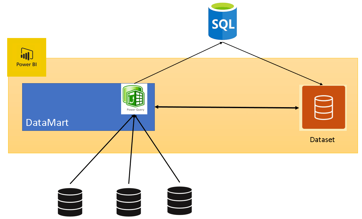
The Datamart uses an underlying Azure SQL Database to store its data. This creates very powerful possibilities. When creating a Datamart, you can import the data from many different sources to this Azure SQL Database using Power Query. The Datamart will also automatically create and manage a dataset linked to the internal Azure SQL Database.

Some architectural details:

• The dataset model is built on the Datamart
• Renaming the Datamart renames the dataset
• The tables in the dataset use direct query but have support for caching, which is done transparently for us
• It also supports dataflows as sources
• You have limited control over the settings of the dataset
• You have very limited control over the underlying Azure SQL Database. It’s provisioned by Power BI.

After learning about the architecture, here are the main features you can expect from the Power BI Datamart:

• It provides a UI to build a data mart in the portal
• This UI is basically the use of Power Query to import data. The portal doesn’t support the use of Power Query with datasets, you need to use Power BI desktop.
• Using Datamarts, you can build Power Query ETLs using the portal. The data imported by Power Query will be saved in the Azure SQL Database
• You can build a model using the imported tables.
• You can define relationships, create measures, and configure the attributes and tables.
• The UI provides additional resources for exploratory analysis
• The Datamart UI provides data exploration features

There are two new tabs, one for query design, another one for SQL. On both tabs you can explore the data to discover useful information in your data.

The UI also allows you to download the query results to Excel, to expand the exploratory analysis possibilities

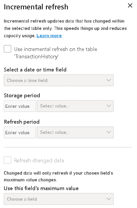
• Support for incremental refresh

Incremental refresh is essential for big tables, and they are expected in a data mart. The configuration is very similar to the incremental refresh configuration you may already know, but the data is being inserted in the Azure SQL Database.

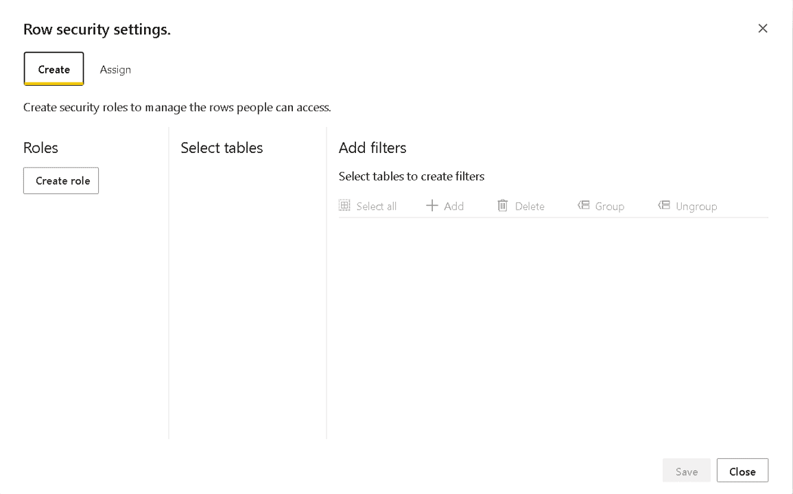
• Support for role-based permissions configuration

• Integrated with Power BI Deployment Pipelines
• Datamarts allow a read-only connection to the Azure SQL Database. This is probably the most powerful tool for exploratory analysis

To understand this new feature, implement a Datamart step-by-step.

Important: The new Power BI feature is called “Datamart”, while the theoretical concept is called “Data mart”.

Implementing a Power BI Datamart

This will be the starting point:

• An Azure SQL Database using the sample AdventureWorskLT
• You need to execute the script Make_big_adventure.SQL adapted for the AdventureWorksLT. You can find it on https://github.com/DennesTorres/BigAdventureAndQSHints/blob/main/make_big_adventureLT.sql
• You need a premium Power BI workspace, either premium by capacity or premium per user
• Recommendation: The Azure SQL Database is recommended to have 10 DTU’s or more. Less than that and some slowness may be noticed
• Recommendation: If you create a non-clustered index on the table BigTransactionhistory, column TransactionDate, the access to the database will be faster.

After preparing the environment, it’s time to start to build the Datamart.

Creating the Datamart: First stage, importing the tables

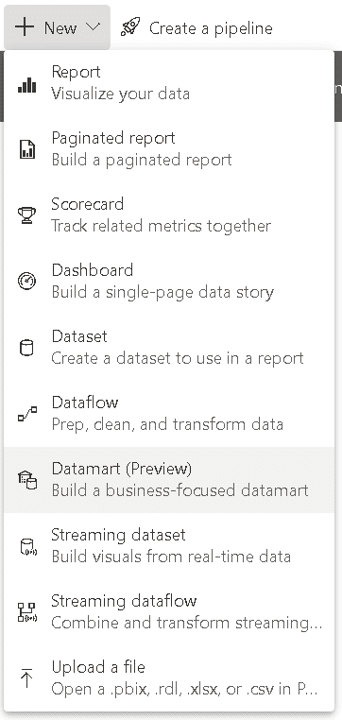
1. In the premium workspace, click New button and select the Datamart menu item

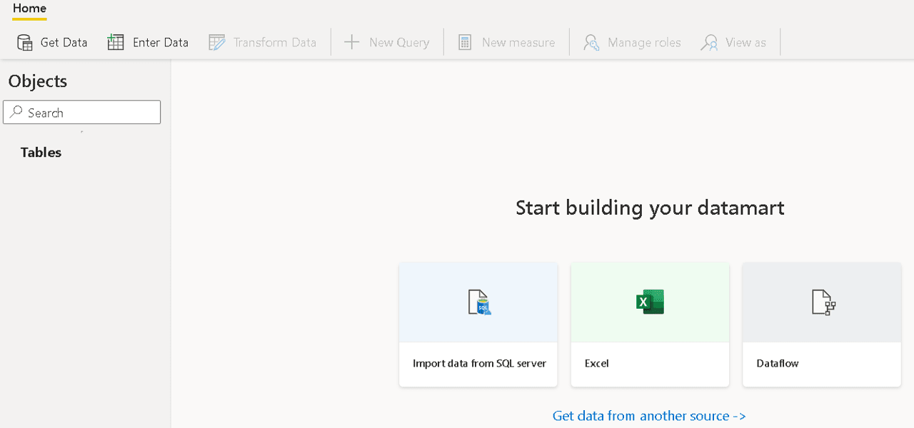
2. On the Datamart design window, click the Import data from SQL Server image in the centre of the screen

Mind you also have options for Excel and Dataflows highlighted, but you also can use the Get Data button and use different kinds of data sources

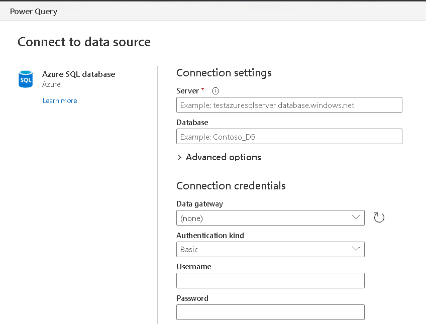
3. In the Connect To Data Source window, fill the Server textbox with the address of your Azure SQL Database
4. On the Connect To Data Source window, fill the Database textbox with the database name
5. On the Connect To Data Source window, fill the user name and password with the Azure SQL Authentication

If your data source were on premises, you could use a gateway for it, but in this case, it’s not needed.

6. Click Next button
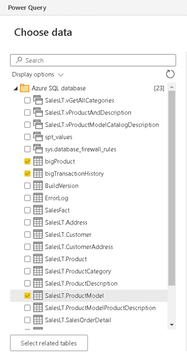
7. On the Power Query window, under Choose Data, select the tables you will include in your Datamart. In this example, include bigTransactionHistory, bigProduct and SalesLT.ProductModel

8. Click the Transform data button

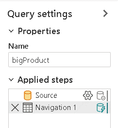
9. On the Power Query window, under Queries, click the table bigProduct

10. On the Query Settings tab, rename it to Product

11. Repeat the steps to rename the table bigTransactionHistory to TransactionHistory
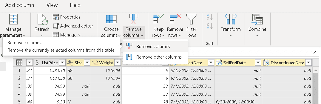
12. Select the Product table
13. Select the columns Size, Weight, SellStartDate, SellEndDate and DiscontinuedDate
14. Use the button Remove Column to remove the unneeded columns

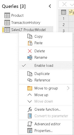
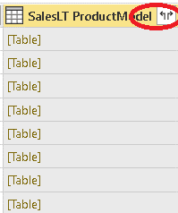
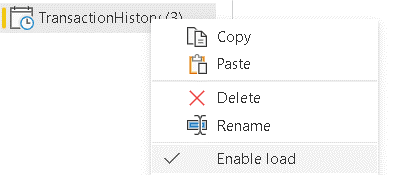
15. Right-click the table SalesLT ProductModel
16. Disable the option Enable Load

You will merge the information about the product model with the product details. You don’t need the ProductModel table as part of the model. When the Enable Load is disabled, the name of the table appears in Italic among the queries

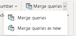
17. Select the table Product
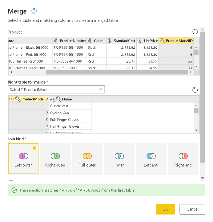
18. Click the Merge queries button

19. On the Merge window, on the Right table for merge, select the table SalesLT ProductModel
20. On the Merge window, Product table, select the ProductModelID field
21. On the Merge window, SalesLT ProductModel table, select the ProductModelID table

22. Once the match message appears in a green bar on the lower side of the window, click the Ok button
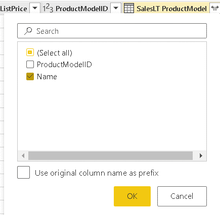
23. On the new SalesLT ProductModel column, click the expand button

24. On the window opened from the expand button, select the Name field, and uncheck all the others

25. Click the OK button
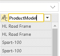
26. Double click the Name.1 column header and change the name to ProductModel

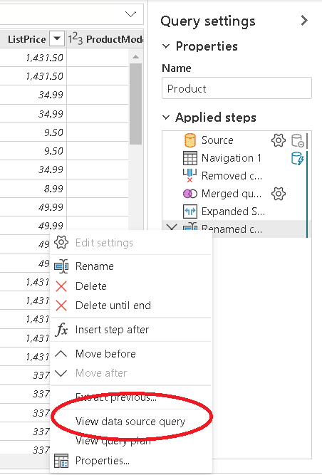
All the steps executed so far are registered on the properties window, Applied Steps. This is exactly how Power Query works, but until now this experience was available only on dataflows or in Power BI desktop.

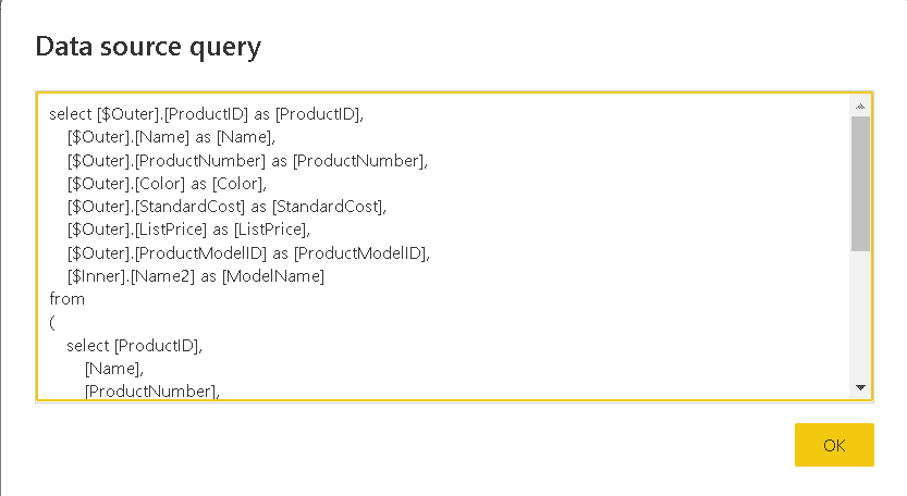
One important performance detail about the steps is to know if the steps will be executed in the source database, converted into a single native query on the source database, or if the sequence of transformations prevent this.

The usual way to check this is to right click the last transformation and check if the option View Data Source Query is available. If it’s available, it means the transformations are good enough to be executed as a single native query.

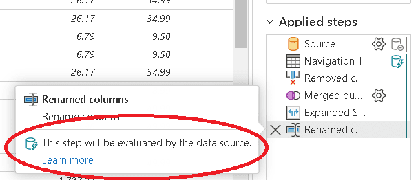
The UI in the portal has some additional features beyond the desktop UI. If you move the mouse over the last step, it tells you how the step will be executed. You can see the same on every step.

Creating the Datamart: Second stage, creating a date dimension

A model needs a date dimension. Every fact happens on a date and the date is an important dimension to analyse the fact. In this example, the TransactionDate column is found in the TransactionHistory table.

Why is the TransactionDate field is not enough, you may ask.

When analysing the facts, it might be analyzed by Year, Month, Day, Day of the week, and much more. If relying only on the TransactionDate field, you will need to create DAX measures, and this would impact the performance of your model.

Building a date dimension, which will be stored in the underlying Azure SQL Database for the Datamart, you will not have the need to build so many DAX expressions and the model will have better performance.

You could say there is a “not so old saying” about this: The better the underlying model, the fewer custom DAX expressions will be needed to build in the model. The date dimension is one great example of this, and the Datamart brings the possibility to create a better underlying model, leaving the DAX expressions only for dynamic calculations which really can’t be created in the underlying model.

There are many different methods to create a date dimension. In this example, I will use the M scrips created by Chris Webb on the following blog: https://blog.crossjoin.co.uk/2013/11/19/generating-a-date-dimension-table-in-power-query/

Execute these step-by-step directions to create the date dimension:

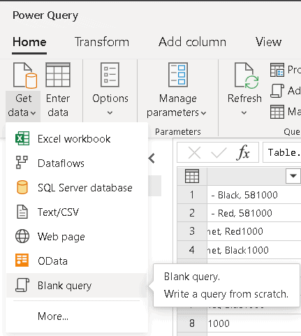
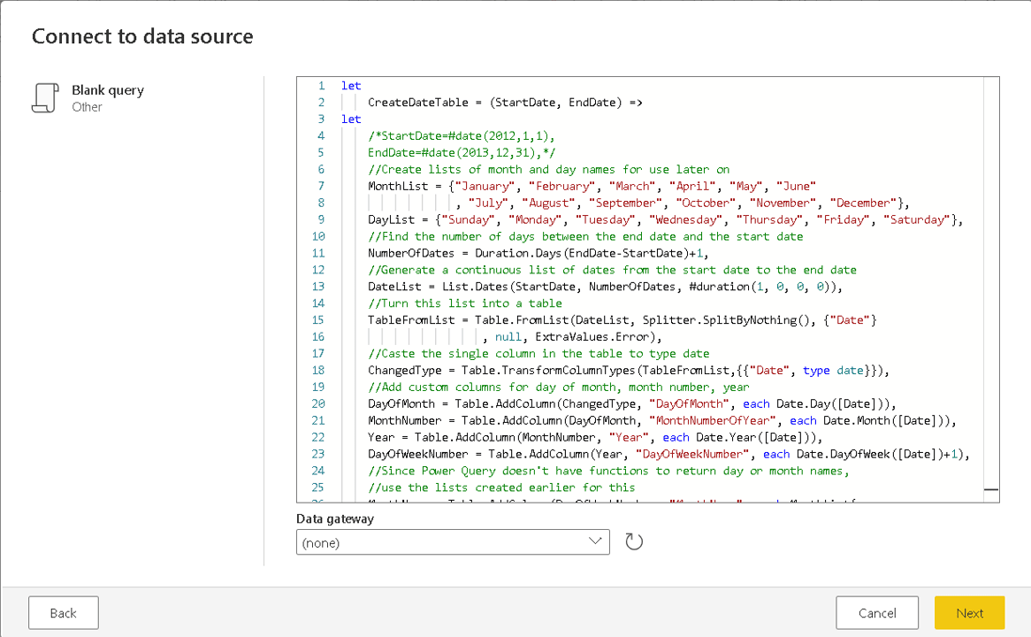
27. On the top menu, click New Query -> Blank Query

28. Paste the query copied from Chris Webb’s blog above

29. Click Next button
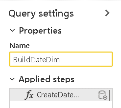
30. In the Properties window, change the name of the new query to BuildDateDimension

You may notice this query is in fact a custom M function. The details about custom M functions are beyond this article, but you can learn more about them watch the recording of some technical sessions about advanced ETL with power query: https://www.youtube.com/watch?v=IjLlqTdF2bg&list=PLNbt9tnNIlQ6s597rRyoGx_sLn4rrHOzv

This function requires two parameters, StartDate and EndDate, to build the date dimension. You can provide these parameters dynamically, so you will always have an updated date dimension. On the next steps, retrieve these values from the TransactionHistory table.

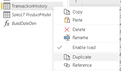
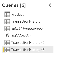
31. Right click the TransactionHistory table and click the Duplicate option in the context menu

32. Repeat the previous step, resulting in two copies of the TransactionHistory table.

Why duplicate and not reference? Since all the transformations will be converted to native queries anyway, duplicating makes it easy to convert each of the queries into an independent native SQL query. If you use reference, future changes to the source query would affect the new query.

I wrote a blog post exactly about this example, you can read more on https://ift.tt/NKvsbcW. 

33. Select the first duplicated query
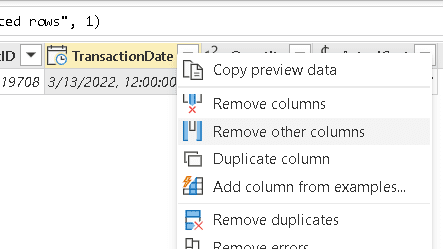
34. Select the TransactionDate field
35. Right-click the column header and click the Remove other columns in the context menu

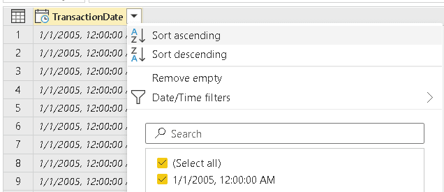
36. Click the button on the TransactionDate header
37. Click the Sort Ascending menu item

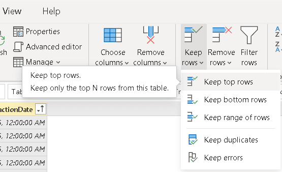
38. Click the Keep top rows menu item

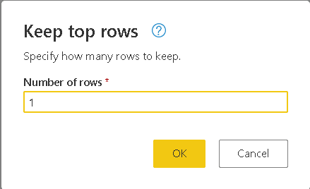
39. On the Keep to Rows window, type 1

40. Click the Ok button
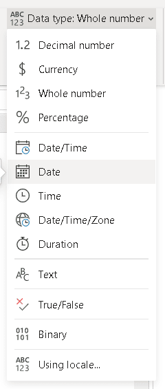
41. On the top menu, change the data type to Date

A date dimension should never include time. If your business needs time, you would need to create a time dimension and include date and time information in different fields

However, these sample tables don’t include time, so changing the data type just ignores the time.

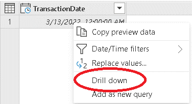
42. Right-click the date value and select the item Drill down on the context menu

Even after reaching a single value, the result is still a table. The parameter for the function, on the other hand, needs to be a value. Using the Drill down option you are retrieving the date as a single value

43. Right-click the duplicated table you are working with and disable the option Enable Load

This query will be used only as parameter for the function, you don’t need it in the model. Besides this, if you don’t disable the load, the Power Query UI will convert the single value to table again, adding a new step to the query.

44. Repeat the steps 33-43 for the 2^nd duplicated query, but this time sorting the data in descending order
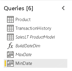
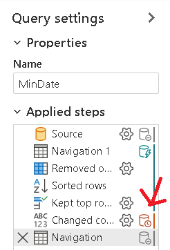
45. Click the first duplicated table and rename it to MinDate
46. Click the second duplicated table and rename it to MaxDate

The steps of these queries show some additional features. On the image below you may notice a red database symbol besides one step. This means that step will not be transformed into the native data source query. As a result, all the steps after it will also not be part of the native data source query, they will be executed by Power BI.

On this example, these are the last steps, conversion of the last value retrieved, so there is no problem at all

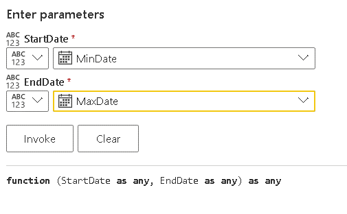
47. Select the BuildDateDimension function
48. On the button besides the StartDate parameter, change the option to query
49. On the StartDate drop down, select the MinDate query
50. On the button besides the EndDate parameter, change the option to query
51. On the EndDate drop down, select the MaxDate query

52. Click the Invoke function

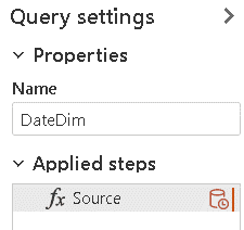
A new query will be created using the M code needed to invoke the function, what will produce the date dimension

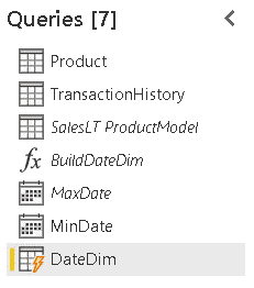
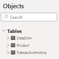
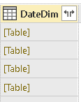
53. Rename the new query as DateDim

54. Click the Save button

After clicking the save button, the data will be loaded into the Datamart.

Renaming the Datamart

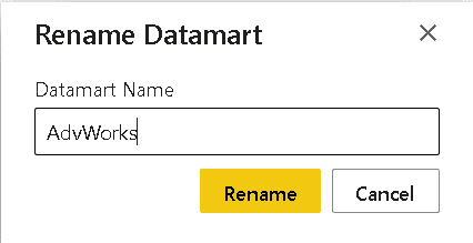
The Datamart is created with an auto-generated name. At some point you would like to rename the Datamart.

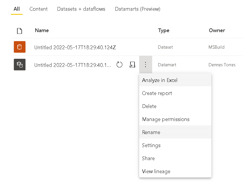
Clicking on the workspace name in the list of workspaces on the left side, you will see the Datamart and the auto-generated dataset.

On the Datamart menu, you will find a Rename command.

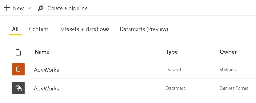
Once you rename the Datamart, the auto-generated dataset will be renamed at the same time.

Building the model

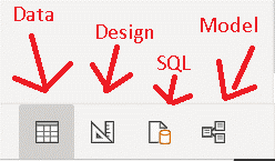
The fourth tab on the lower toolbar inside the Datamart is the Model tab. On this tab, you can make model configurations for the tables. It’s time to build the model.

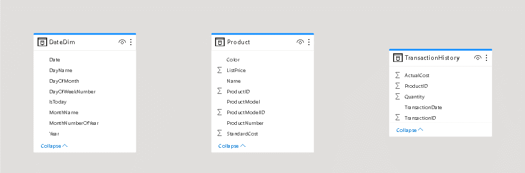
55. Click the Model tab

56. Organize the tables, leaving the fact table, TransactionHistory, in the middle.
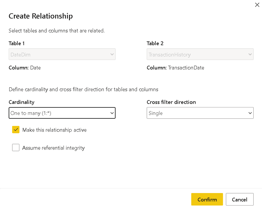
57. Drag the Date field from DateDim table to the TransactionDate field in the TransactionHistory table
58. On the Create Relationship window, adjust the cardinality of the relationship. It needs to be 1 to many from DateDim to TransactionHistory

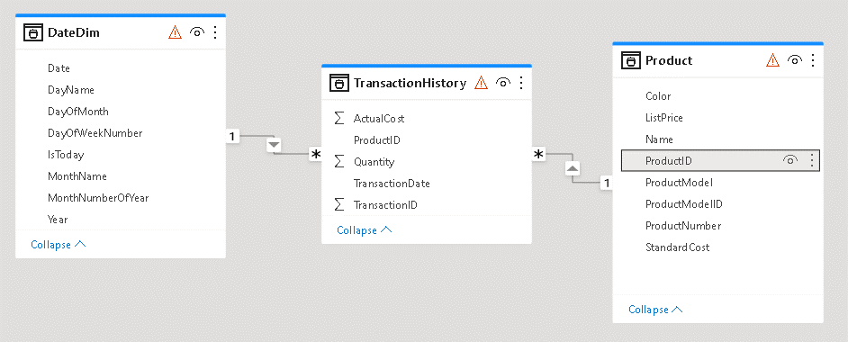
59. Drag the ProductId field from the Product table to the ProductId field on the TransactionHistory table
60. On the Create Relationship window, adjust the cardinality of the relationship. It needs to be 1 to many from Product to TransactionHistory

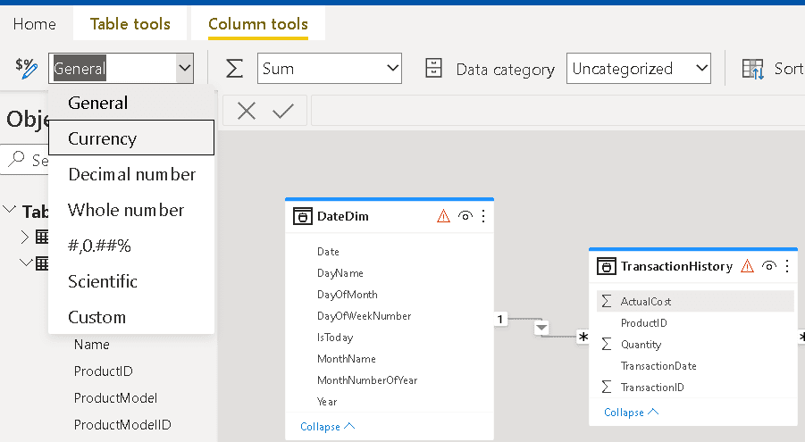
61. Select the ActualCost field in the TransactionHistory table
62. On the top toolbar, change the format of the field to Currency

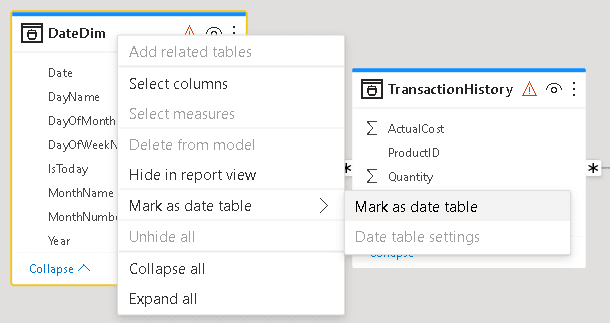
63. Right click the DateDim table and click the menu item Mark as Date Table

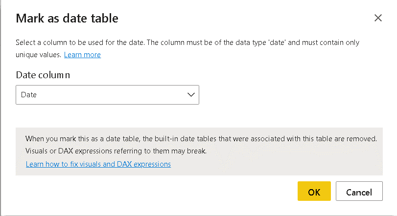
64. On the Mark as Date Table window, select the Date field

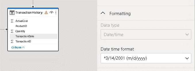
65. Select the TransactionDate field in the TransactionHistory table.
66. On the Properties window located on the right side, under Formatting, select the date format containing only the date

67. Select the Date field in the DateDim table
68. On the properties window located on the right side, under Formatting, select the date format containing only the date

The newly built model will be stored in the auto-generated dataset created together in the Datamart. This dataset can become the base model for all users of the Datamart. Of course, there are many modelling features still missing, such as hierarchies and aggregation tables, but it’s a good start.

Exploratory Analysis: The Design tab

The Design tab is one of the two tabs available to allow exploring the data in the Datamart. Here’s a small example:

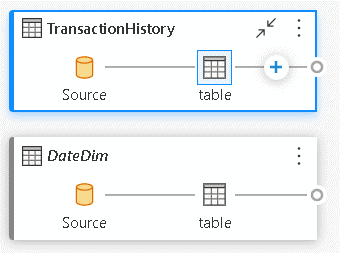
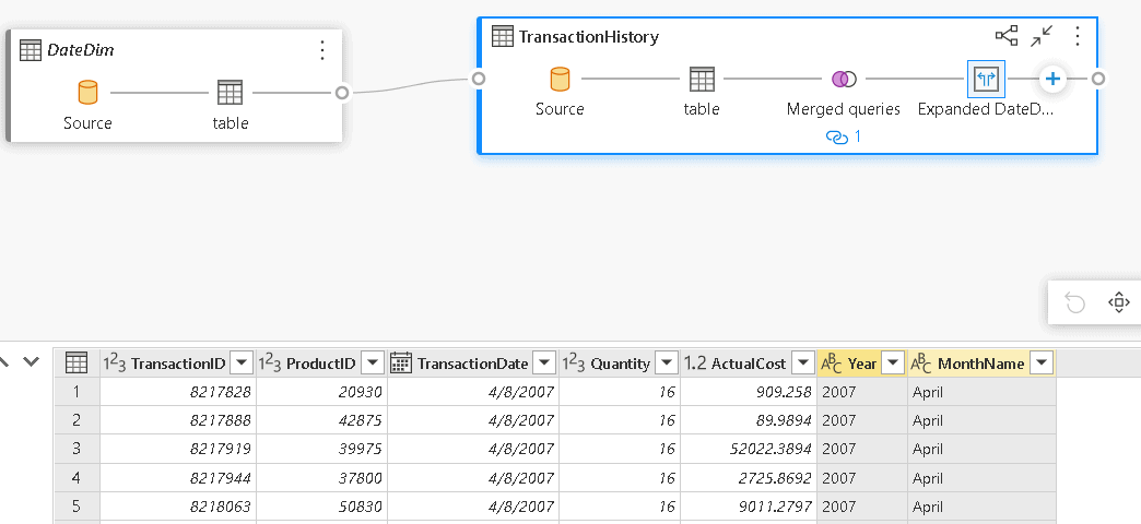
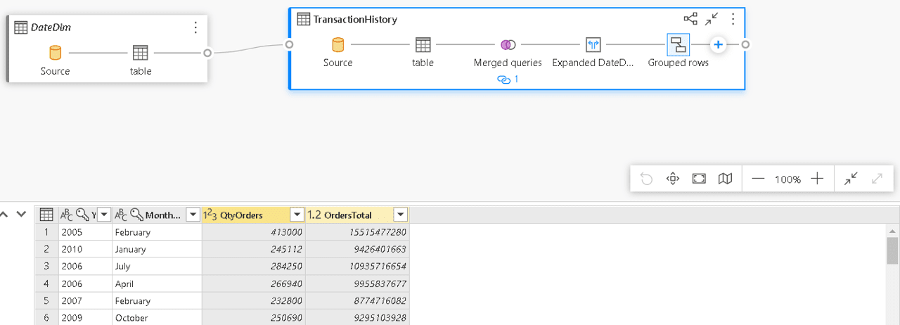
69. Drag the TransactionHistory table to the middle of the Design tab
70. Drag the DateDim table to the middle of the Design tab

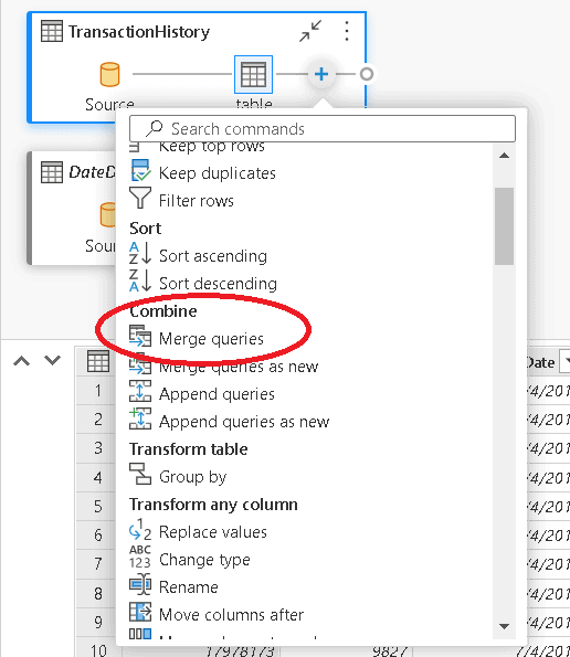
71. Click the “+” sign on the TransactionHistory table and select the Merge queries option

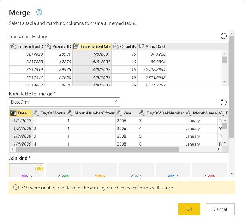
72. On the Merge window, under the Right table for merge, select the DateDim table
73. On the Merge window, in the TransactionHistory table, select the TransactionDate field
74. On the Merge window, in the DateDim table, select the Date field
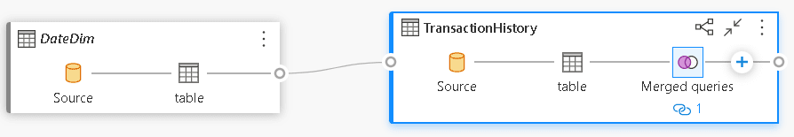
75. Click the Ok button

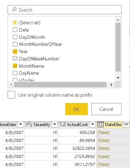
76. On the lower window with the table visualization, click the Expand button besides the new DateDim column

77. On the window with the field names to expand, uncheck all the fields and check only Year and MonthName

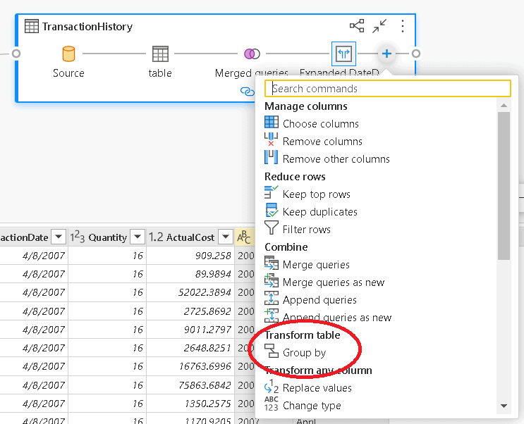
78. On the merged query, click the “+” sign and select the Group By option

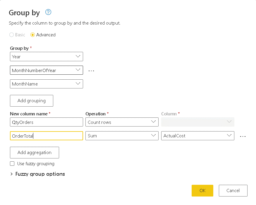
79. On the Group By window, select the option Advanced
80. On the Group By window, click the Add Grouping button once to complete 3 grouping fields
81. On the Group By window, click the Add aggregation button once to complete 2 aggregation fields
82. On the Group By window, select Year, MonthNumberOfYear and MonthName as the 3 grouping fields
83. Under New Column Name, type QtyOrders
84. On Operation drop down to the right of QtyOrders, select Count Rows
85. On the 2^nd New Column Name, type OrdersTotal
86. On the Operation drop down to the right of OrdersTotal, select Sum
87. On the Column drop down, to the right of Sum operation, select ActualCost

88. Click Ok button

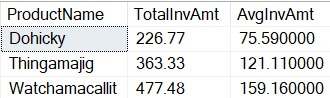
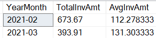
As a result, you have the total of the orders by month

Exploratory Analysis: The SQL tab

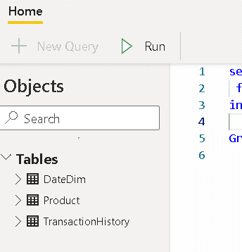
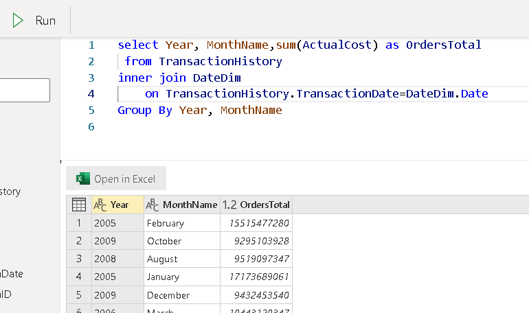
The 2^nd tab which allows exploratory analysis is the SQL table. You can execute SQL statements over the Datamart

Type the following statement on the SQL tab:

select Year, MonthName,sum(ActualCost) as OrdersTotal
 from TransactionHistory
inner join DateDim
    on TransactionHistory.TransactionDate=DateDim.Date
Group By Year, MonthName

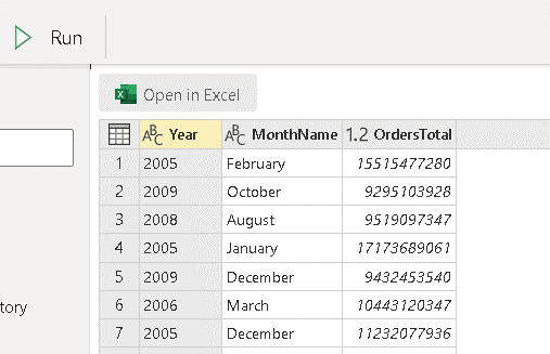
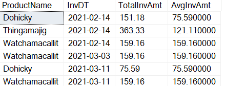
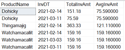
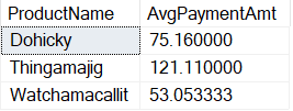
Click the Run button to execute the query

At the moment I’m writing this article, the results window still has a small secret. You can view the results together with the SQL statement, but you need to resize the window from top to bottom for that.

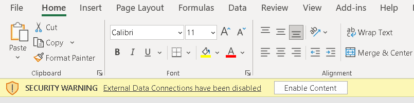
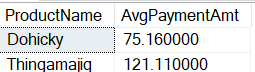
The user can click the Excel button to open the query result in Excel

An Excel file will be downloaded. Once you open it, you will need to click the button Enable Editing. After that, a second message will appear, and you will need to click the button Enable Content.

Excel will connect directly to the Azure SQL Database and execute the query. The user using Excel needs permission to connect to the underlying Azure SQL Database.

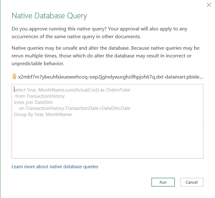
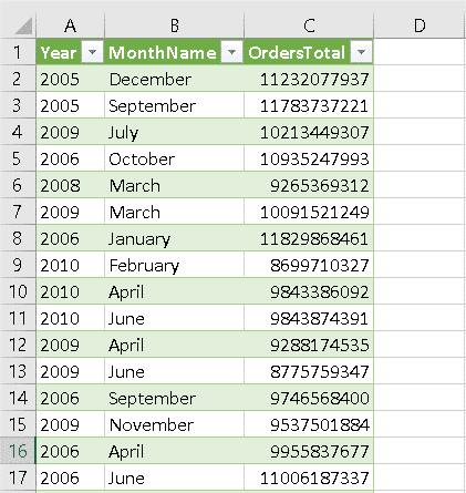
On the Native Database Query window, click the Run button. The query will be executed, and the result inserted in Excel.

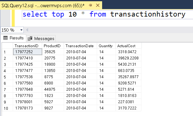
Yes, you have access to SQL

The Power BI Datamarts underlying technology is an Azure SQL database. After all the exploratory analysis features mentioned above, the icing on the cake is a direct connection to Azure SQL Database.

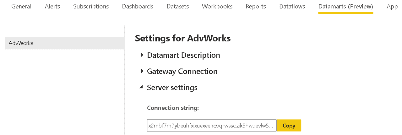
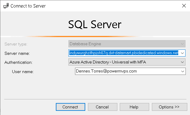
First, you need to locate the connection string for the Azure SQL Database. In the Datamart settings, under Server Settings, you can find the connection string and copy it to be used for connection in another application. For example, you can use SSMS, paste this connection on SSMS connection string to access the Azure SQL Database.

The authentication is made with Active Directory – Universal with MFA. The login is the Power BI login.

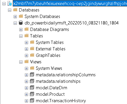
You may notice there are no tables in the database, only views. All the tables created in the model appear as views. The database is completely read only, but the ability to connect to the Datamart using any tool capable to connect to SQL is a very powerful feature.

On my blog about Power BI and ETL, one of my arguments was the fact the ETL in Power BI was only capable to save the data to Power BI. The evolution of the technology always makes the borders between different technologies more difficult to find. I may need to update that article soon.

Using the Datamart to build reports

The Datamart should become the central single source of truth for one area of the company. Whether the Datamart is built using a top-down or bottom-up approach, it’s still a central single source of truth.

For example, if the Datamart is using the bottom-up approach, it will be the central point to integrate all user’s data sources, such as excel, sharepoint lists and many kinds of data sources starting from a small spreadsheet and growing in an uncontrolled rate. It will not be the central point for the entire company, but for one company branch, for example.

On the other hand, in a top-down approach the Datamart is built as a subset of the company data warehouse. This subset may be focused on one branch, and it will be the single source of truth to this branch.

These are some important points which makes the Datamart a good local single point of truth:

• Calculations which in other ways would be made using DAX formulas and turn the model slower, can be done using physical tables and result in a better model
• The model stored in the auto-generated dataset can be used as a base for all local reports and additional models.
• There are many features for exploratory analysis, including direct SQL access to the data

There are three different methods to use the Datamart:

• Use the portal to create reports based on the auto-generated dataset

The reports will be using the auto-generated dataset directly. Depending on the number of different departments using the auto-generated dataset, this may not be the best solution

• Create reports directly accessing the underlying Azure SQL connection

This is a very good solution, but every report solution using this direct connection would need to build the model again, without re-using the model already built in the auto-generated dataset

• Use Power BI desktop to create reporting solutions using the auto-generated dataset as a source

This is probably the best solution for the use of the Datamart. You will be able to re-use the model built in the auto-generated dataset and customize it with additional information needed.

Summary

The Datamarts are more than a very powerful feature, it’s also a critical point in the Power BI evolution. More consistent data exploration tools and consistent tools to create a local single source of truth. It has the potential to change the architectures used to build in Power BI, and I believe everyone all will be looking forward to the new features to come.

 

The post Datamarts and exploratory analysis using Power BI appeared first on Simple Talk.

from Simple Talk https://ift.tt/ZOizBoW
via