Creating Azure Policy to setup Virtual Machine Auto-Shutdown

 The Auto-Shutdown policy is another important policy to ensure our virtual machines don’t expend more than what we planned for them. If we have a time window to use the virtual machines, the auto-shutdown policy can deactivate them at the right time.

We need to discover the deep internal details about the auto-shutdown configuration before creating the policy. The method we can use is to set this configuration and export the virtual machine as a template. We change the configuration to on and off, export and check the difference.

After testing the export template you will discover that Azure creates an object of type Microsoft.DevTestLab/schedules when the auto-shutdown configuration is defined. Azure creates this object the first time we enable the auto-shutdown configuration. However, when we disable it, Azure doesn’t drop the object, it only disables it. Azure enables the existing object again when the auto-shutdown configuration.

Schedules and Properties

We need to check the Microsoft.DevTestLab/schedules. We will test the property targetResourceId to ensure the schedule belongs to the correct machine machine and the status property to check if the schedule object is enabled or not.

The policy require us to use the full name of the fields. The documentation about the full name of the fields is not always available. It’s a challenge to find them. After a lot of research, I discovered the full name of the fields:

Status: Microsoft.DevTestLab/schedules/status

TargetRersourceId: Microsoft.DevTestLab/schedules/targetResourceId

A few weeks ago I wrote about parameterizing Azure policies. We can apply the same concepts to the auto-shutdown policy. The local IT teams will choose to enable the auto-shutdown configuration automatically or only audit when the configuration is enabled or not. The policy will allow them to choose between AuditIfNotExists or DeployIfNotExists

The policy will be like this:

{
     "parameters": {
          "effect": {
            "type": "String",
            "metadata": {
              "displayName": "Effect",
              "description": "Enable or disable the execution of the policy"
            },
            "allowedValues": [
              "DeployIfNotExists",
              "auditIfNotExists",
              "Disabled"
            ],
            "defaultValue": "DeployIfNotExists"
          }
     },
     "policyRule": {
       "if": {
         "allOf": [
           {
             "field": "type",
             "equals": "Microsoft.Compute/virtualMachines"
           }
         ]
       },
       "then": {
         "effect": "[parameters('effect')]",
         "details": {
           "type": "microsoft.devtestlab/schedules",
           "roleDefinitionIds": [
             "/providers/Microsoft.Authorization/roleDefinitions/9980e02c-c2be-4d73-94e8-173b1dc7cf3c"
           ],
           "existenceCondition": {
             "allOf": [
               {
                 "field": "Microsoft.DevTestLab/schedules/targetResourceId",
                 "equals": "[field('id')]"
               },
               {
                 "field": "Microsoft.DevTestLab/schedules/status",
                 "equals": "Enabled"
               }
             ]
           },
           "deployment": {
             "properties": {
               "mode": "incremental",
               "name": "Default",
               "template": {
                 "$schema": "https://schema.management.azure.com/schemas/2019-04-01/deploymentTemplate.json#",
                 "contentVersion": "1.0.0.0",
                 "parameters": {
                   "vmName": {
                     "defaultValue": "devMaltaStation",
                     "type": "String"
                   }
                 },
                 "variables": {
                   "rId": "[resourceId('Microsoft.Compute/virtualMachines', parameters('vmName'))]",
                   "schName": "[concat('shutdown-computevm-',parameters('vmName'))]"
                 },
                 "resources": [
                   {
                     "type": "Microsoft.DevTestLab/schedules",
                     "apiVersion": "2018-09-15",
                     "name": "[variables('schName')]",
                     "location": "northeurope",
                     "properties": {
                       "status": "Enabled",
                       "taskType": "ComputeVmShutdownTask",
                       "dailyRecurrence": {
                         "time": "0000"
                       },
                       "timeZoneId": "Central European Standard Time",
                       "notificationSettings": {
                         "status": "Disabled",
                         "timeInMinutes": 30,
                         "notificationLocale": "en"
                       },
                       "targetResourceId": "[variables('rId')]"
                     }
                   }
                 ]
               },
               "parameters": {
                 "vmName": {
                   "value": "[field('name')]"
                 }
               }
             }
           }
         }
       }
     }
}

Once created and assigned, you can check the policy to verify the result or apply remediation. I wrote a bit about this on the blog about evaluating Azure Policy tenant-wide

 

Summary

The auto-shutdown policy is one more important policy we should use in our Azure environment. Making it as a parameterized policy is one additional benefit for our environment.

 

The post Creating Azure Policy to setup Virtual Machine Auto-Shutdown appeared first on Simple Talk.

from Simple Talk https://ift.tt/V16GfHL
via

Let’s talk about salary

Said no manager ever.

Money is the one thing every candidate at any job interview is advised never to mention. The salary on offer for the role is treated almost like a *dirty secret. Job advertisements only reveal a band or range, which makes sense to a certain extent, given that the candidate may be placed at any point within that band, depending on experience and qualifications. However, in places like Germany, jobs are advertised without a hint of what the monetary compensation will be. You could be applying to a role at anything from 50% less to 40% more than your current salary, you’d never know. Not even after the interviews, because, well, see *above. In short, you never know what you’re getting until HR get back to you with an actual offer.
What’s worse, your current salary plays a critical role in setting your future salary. Even after having cleared several hoops and umpteen rounds of interviews, discussions, and negotiations, having had your qualifications thoroughly scrutinised and references painstakingly checked, having been deemed to be the best person for the job, leaving behind all competition, you must
still reckon with The HR Policy, which insists on anchoring you to your past income and decrees a cap on your compensation. It’s not just a line in the sand; it is a veritable canyon that cannot be crossed.

Just imagine it. Some statement written in some document by some person somewhere has the power to determine your earning potential, your career path, your future life. You will never meet that person, you will never even set eyes on that document, but it will hold you down “in your place,” where you belong.

A job is a business transaction: the employee gives hours of their life and skills to further the business of the employer, while the employer compensates them for it with a salary. A job may be made pleasant if one enjoys one’s work; otherwise, it is nothing more than a way to earn money to live. It is the main Return on Investment for an employee. Then why are employees advised never to ask about salaries in job interviews? Why wouldn’t you want to know the most important thing that’s in it for you? Why is salary such a taboo topic? Who has decided that it is a subject that must never be raised lest the candidate be seen as some kind of money-grabbing mercenary lacking commitment?

Let us change the paradigm. Let us agree that asking about money in an interview is not wrong. It is not disrespectful. It is not greedy. It has nothing to do with commitment, engagement, or loyalty. It is simply a basic Right and one which companies must embrace as openly as they
do other things: things that fetch more PR brownie points, like Diversity, Equality, and Sustainability.

Make Money Normal Again.

Commentary Competition

Enjoyed the topic? Have a relevant anecdote? Disagree with the author? Leave your two cents on this post in the comments below, and our favourite response will win a $50 Amazon gift card. The competition closes two weeks from the date of publication, and the winner will be announced in the next Simple Talk newsletter.

The post Let’s talk about salary appeared first on Simple Talk.

from Simple Talk https://ift.tt/KkvZ52U
via

What’s new in T-SQL in SQL Server 2022

There are many new features in SQL Server 2022. In relation to T-SQL querying, there are a few as well and they usually are left for last in face of many other new optimization features.

Sample scenario

These samples are built on the AdventureWorksDW2019 database installed in a SQL Server 2022 CTP 2.

Date_Bucket

Let’s first consider a sample query. The following query shows information about internet sales and products.

SELECT p.productkey,
       englishproductname,
       orderdate,
       salesamount
FROM   dimproduct p
       INNER JOIN factinternetsales fi
               ON p.productkey = fi.productkey 

 

The Date_Bucket function, as the name implies, calculates date buckets of one specific size. Given a date and the bucket size, the function will return the start date of the bucket containing the date.

This is very useful to classify the facts in our data in groups according a date bucket. For example, we can create 2 weeks bucket, 2 months bucket and so on. The date bucket function is useful for grouping on these scenarios.

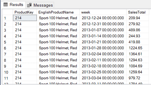
For example, based on the query above, let’s create a 1 week date bucket to group the product sales.

SELECT p.productkey,
       englishproductname,
       Date_bucket(week, 1, orderdate) week,
       Sum(salesamount)                AS SalesTotal
FROM   dimproduct p
       INNER JOIN factinternetsales fi
               ON p.productkey = fi.productkey
GROUP  BY p.productkey,
          englishproductname,
          Date_bucket(week, 1, orderdate)
ORDER  BY productkey,
          week 

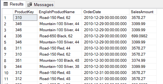
If we change the size of the bucket to 2 weeks, instead of one, you may notice on the following image the dates organized for each two weeks.

The calculation of the buckets needs a starting point. This is an optional parameter. When we don’t specify the starting point, the calculation starts on 01/01/1900. That’s how it was calculates on the previous two queries.

There is no surprise the Date_Bucket expression is not a SARG. As you may notice on the execution plan below, the index operations are all SCAN.

 

The query plan complains about some missing indexes. Let’s create them first and analyse the impact of Date_bucket isolated from other needs in the query.

CREATE INDEX indprodkey
  ON dimproduct(productkey)

CREATE INDEX indfactprodkey
  ON factinternetsales(productkey)
  include (orderdate, salesamount) 

After these indexes are created, the query plan will be like this one below:

 

Let’s execute the follow statements followed by the query execution to get a clean statistics. Don’t do this in a production environment.

SET statistics time ON
SET statistics io ON

DBCC freeproccache

DBCC dropcleanbuffers 

SQL Server parse and compile time:
CPU time = 0 ms, elapsed time = 55 ms.

(3959 rows affected)
Table ‘Worktable’. Scan count 0, logical reads 0, physical reads 0, page server reads 0, read-ahead reads 0, page server read-ahead reads 0, lob logical reads 0, lob physical reads 0, lob page server reads 0, lob read-ahead reads 0, lob page server read-ahead reads 0.
Table ‘FactInternetSales’. Scan count 1, logical reads 345, physical reads 0, page server reads 0, read-ahead reads 344, page server read-ahead reads 0, lob logical reads 0, lob physical reads 0, lob page server reads 0, lob read-ahead reads 0, lob page server read-ahead reads 0.
Table ‘DimProduct’. Scan count 1, logical reads 6, physical reads 1, page server reads 0, read-ahead reads 11, page server read-ahead reads 0, lob logical reads 0, lob physical reads 0, lob page server reads 0, lob read-ahead reads 0, lob page server read-ahead reads 0.

SQL Server Execution Times:
CPU time = 47 ms, elapsed time = 112 ms.

There are two solutions to improve the performance with the Date_Bucket function:

• If the Buckets match with information in a date dimension, using the date dimension instead of date_bucket will perform better. Leaves the date_bucket function for buckets which don’t match with information in the date dimension.
• If the bucket is used very often, create a calculated field and uses it in an index.

Considering the indexes we created before, the code to create and use the calculated field will be like this:

ALTER TABLE factinternetsales
  ADD twoweeksbucket
       AS Date_bucket(week, 2, orderdate) persisted
go

DROP INDEX factinternetsales.indfactprodkey
go

CREATE INDEX indfactprodkey
  ON factinternetsales(productkey, twoweeksbucket)
  include (salesamount)
go 

The new query will need to use the calculated field. The new query plan changes the location of the stream aggregate and the cost of the SORT is very reduced. We need to check the statistics and time to compare the new query with the old one.

SELECT p.productkey,
       englishproductname,
       twoweeksbucket   week,
       Sum(salesamount) AS SalesTotal
FROM   dimproduct p
       INNER JOIN factinternetsales fi
               ON p.productkey = fi.productkey
GROUP  BY p.productkey,
          englishproductname,
          twoweeksbucket
ORDER  BY productkey,
          week 

SQL Server parse and compile time:
CPU time = 31 ms, elapsed time = 64 ms.

(3959 rows affected)
Table ‘Worktable’. Scan count 0, logical reads 0, physical reads 0, page server reads 0, read-ahead reads 0, page server read-ahead reads 0, lob logical reads 0, lob physical reads 0, lob page server reads 0, lob read-ahead reads 0, lob page server read-ahead reads 0.
Table ‘FactInternetSales’. Scan count 1, logical reads 405, physical reads 0, page server reads 0, read-ahead reads 409, page server read-ahead reads 0, lob logical reads 0, lob physical reads 0, lob page server reads 0, lob read-ahead reads 0, lob page server read-ahead reads 0.
Table ‘DimProduct’. Scan count 1, logical reads 6, physical reads 1, page server reads 0, read-ahead reads 11, page server read-ahead reads 0, lob logical reads 0, lob physical reads 0, lob page server reads 0, lob read-ahead reads 0, lob page server read-ahead reads 0.

SQL Server Execution Times:
CPU time = 15 ms, elapsed time = 68 ms.

The CPU time and Elapsed Time improved a lot from the original query.

You can read more about Date_Bucket here

Window Expression

The window functions and OVER expressions are present since SQL Server 2018. Now we have a new expression to make it easier to write these queries.

The OVER expression allows us to retrieve detail data about the rows and aggregated data at the same time.

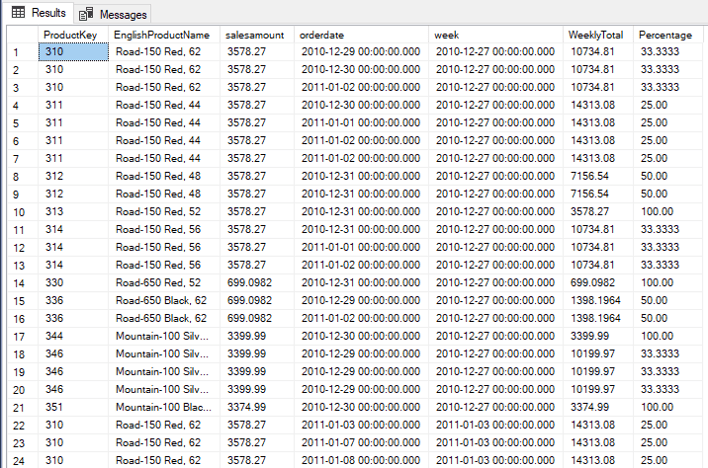
For example, considering the previous example using date_bucket, we can bring the details of each transaction and the total of the week bucket. We also can make a percentage calculation comparing each transaction with the bucket’s total

The query will be like this:

SELECT p.productkey,
       englishproductname,
       salesamount,
       orderdate,
       Date_bucket(week, 1, orderdate) week,
       Sum(salesamount)
         OVER (
           partition BY p.productkey, Date_bucket(week, 1, orderdate))
       WeeklyTotal,
       100 * salesamount / Sum(salesamount)
                             OVER (
                               partition BY p.productkey, Date_bucket(week, 1,
                             orderdate)) Percentage
FROM   dimproduct p
       INNER JOIN factinternetsales fi
               ON p.productkey = fi.productkey
ORDER  BY week,
          productkey,
          orderdate 

 

The new WINDOW expression allows us to simplify the query by writing the WINDOW expression once, in the end of the query, and referencing it where it’s needed, even more than once.

Using the WINDOW expression, the query will be like this:

SELECT     p.productkey,
           englishproductname,
           salesamount,
           orderdate,
           Date_bucket(week,1,orderdate)                 week,
           sum(salesamount) OVER win                     weeklytotal,
           100 * salesamount / sum(salesamount) OVER win percentage
FROM       dimproduct p
INNER JOIN factinternetsales fi
ON         p.productkey=fi.productkey window win AS (partition BY p.productkey, date_bucket(week,1,orderdate))
ORDER BY   week,
           productkey,
           orderdate

 

The queries will have the same execution plan, the new syntax will not affect the execution, it will only make them easier to read.

You can read more about the window exprpession here: https://docs.microsoft.com/en-us/sql/t-sql/queries/select-window-transact-sql?WT.mc_id=DP-MVP-4014132&view=sql-server-ver16 

LEAST and GREATEST function

These new functions are used to find the smallest and biggest value in a set of values. They are not intended to be used in a set of records, for this we have the MAX and MIN aggregation functions. LEAST and GREATEST are intended to be used in a set of values, for example, a set of fields.

Let’s build one useful example for these functions. We can use the PIVOT statement in SQL Server to transform a rows into columns, comparing the sales of the products in a single quarter, for example.

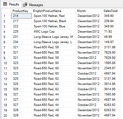
A regular query without using the PIVOT would be like this:

SELECT p.productkey,
       englishproductname,
       englishmonthname + ‘/’
       + CONVERT(VARCHAR, calendaryear) AS Month,
       Sum(salesamount)                 SalesTotal
FROM   factinternetsales fi
       INNER JOIN dimproduct p
               ON fi.productkey = p.productkey
       INNER JOIN dimdate d
               ON fi.orderdatekey = d.datekey
WHERE  d.calendaryear = 2012
       AND d.calendarquarter = 4
GROUP  BY p.productkey,
          englishproductname,
          calendaryear,
          englishmonthname 

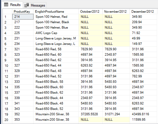
Using the PIVOT on this query we can turn the months into columns:

SELECT productkey,
       englishproductname,
       [october/2012],
       [november/2012],
       [december/2012]
FROM   (SELECT p.productkey,
               englishproductname,
               englishmonthname + ‘/’
               + CONVERT(VARCHAR, calendaryear) AS Month,
               Sum(salesamount)                 SalesTotal
        FROM   factinternetsales fi
               INNER JOIN dimproduct p
                       ON fi.productkey = p.productkey
               INNER JOIN dimdate d
                       ON fi.orderdatekey = d.datekey
        WHERE  d.calendaryear = 2012
               AND d.calendarquarter = 4
        GROUP  BY p.productkey,
                  englishproductname,
                  calendaryear,
                  englishmonthname) AS sales
       PIVOT ( Sum(salestotal)
             FOR month IN ([October/2012],
                           [November/2012],
                           [December/2012]) ) AS pivottable 

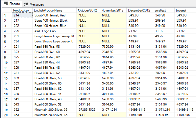
This is a great example to use LEAST and GREATEST to find the smallest and biggest values in a quarter:

SELECT productkey,
       englishproductname,
       [october/2012],
       [november/2012],
       [december/2012],
       Least([october/2012], [november/2012], [december/2012])    smallest,
       Greatest([october/2012], [november/2012], [december/2012]) biggest
FROM   (SELECT p.productkey,
               englishproductname,
               englishmonthname + ‘/’
               + CONVERT(VARCHAR, calendaryear) AS Month,
               Sum(salesamount)                 SalesTotal
        FROM   factinternetsales fi
               INNER JOIN dimproduct p
                       ON fi.productkey = p.productkey
               INNER JOIN dimdate d
                       ON fi.orderdatekey = d.datekey
        WHERE  d.calendaryear = 2012
               AND d.calendarquarter = 4
        GROUP  BY p.productkey,
                  englishproductname,
                  calendaryear,
                  englishmonthname) AS sales
       PIVOT ( Sum(salestotal)
             FOR month IN ([October/2012],
                           [November/2012],
                           [December/2012]) ) AS pivottable 

 

Summary

These are only 3 of the interesting T-SQL improvements in SQL Server 2022

 

 

The post What’s new in T-SQL in SQL Server 2022 appeared first on Simple Talk.

from Simple Talk https://ift.tt/NL1F4HA
via

Boost productivity with ‘Solution Summary’ cards

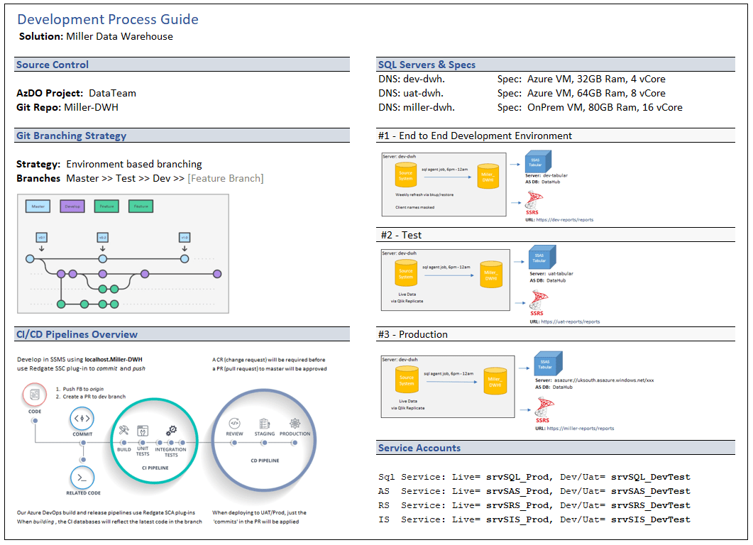
Solution Summary cards are the name I have given to simple 1-page documents we provide to developers to get up-to-speed on a particular solution.

The primary use-case for these cards is to provide better on-boarding for new team members.

An additional benefit is that crafting these short summaries forces people to review how your teams are working and you will often start seeing areas which would benefit from standardization or simplification.   

An example of one these cards, in this case for a simple Data Warehouse implementation, can be seen below:

These cards are not intended to replace full technical guides, but to just capture the essential information that you would often need at a glance and prevent scrolling back and forth through larger documents.

Boost productivity by reducing ‘cognitive load’

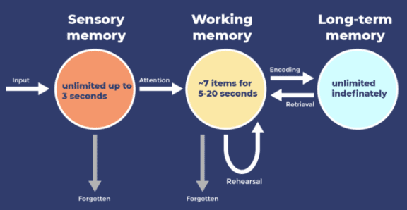
Cognitive load relates to the amount of information your brain can use to figure stuff out.  Since your working memory has a very limited capacity, we should avoid overloading it with unnecessary information.

How working memory fits into the overall cognitive process can be seen in this Information Processing Model.

Developers want to focus on solving real-problems, for real-people, in the real-world.  All the ‘other stuff’ we contend with is just a distraction.

Having to fill up the brain’s mental model with unnecessary information will drain the energy and productivity of your teams. 

For example, we are able to use our cognitive faculties more efficiently if we know we can quickly reference (instead of memorizing) the following information

• Where do I commit or deploy code?
• What happens when I commit?
• How up to date is the data in each environment?
• Which downstream systems will be affected by my changes?

Even without these cards, after a while, people will learn all the server details, processes and nuances – but it comes at a cost in the form of a lot of wasted effort.

Summary

This is not a revolutionary new idea, however, I wanted to share an example of what I do in case it inspires others.

For this work, understanding cognitive load helped me to find the balance between detail and usability. 

There are 3 types of cognitive load and the ultimate goal of these ‘cards’ is to reduce extraneous load.

1. Intrinsic Load      – i.e. The SQL skills required to solve the problem
2. Extraneous Load – i.e. Unnecessary distraction such as a requirement buried within a long chain of emails
3. Germane Load     – i.e. The load required to take information from working memory into long term memory

If you would like to know more, I found the following two resources informative:

YouTube: Hacking Your Head: Managing Information Overload, by Jo Pearce.

Article:  https://www.gerardfriel.com/instructional-design/cognitive-load-theory/

The post Boost productivity with ‘Solution Summary’ cards appeared first on Simple Talk.

from Simple Talk https://ift.tt/tB6h12i
via