Tuesday, January 23, 2024

Querying MongoDB Documents

MongoDB provides an efficient environment for storing document data at scale. However, most of your interactions with MongoDB will not be related to storing data but rather to querying data. The better you understand how to retrieve the data you need, the more effectively you can interact with MongoDB and support your data-driven applications.

To help you get started, this article introduces you to various ways you can query document data in a MongoDB database. I demonstrate how to use both MongoDB Shell and the MongoDB Compass GUI when interacting with your collection data.

Keep in mind, however, that building MongoDB queries is an extensive and many-faceted topic, one that can easily justify multiple articles (if not a book or two). In this article, I introduce you to the basics, with the goal of helping you create a foundation on which you can continue to build. The better you understand the concepts presented here, the more easily you’ll be able to move onto more advanced topics.

Note: For the examples in this article, I used MongoDB Atlas and MongoDB Compass. The last section of this article—“Appendix: Preparing your MongoDB environment”—provides information about how to set up your environment and includes a link to a .json file that you’ll need to download if you want to try out these examples for yourself.

Friday, January 19, 2024

The Importance of Retention

It is always an afterthought. New objects are created that start off small and current. New feature development takes over and the recently architected data structures become old news. Over time, data grows and suddenly a previously small table contains millions or billions of rows.

Is all that data necessary? How long should it be retained for? If there is no answer to this question, then the actuality may be “Forever”, or more honestly “No one knows for sure.”

Retention takes on many forms and this article dives into ways in which data can be managed over time to ensure that it is fast, accurate, and readily available.

Note: the code for this article can be found here.

The Common Scenario

A new feature has been added and it requires verbose logging, which will provide troubleshooting information, as well as useful usage data that can be crunched in the future. The following is how this table might look:

CREATE TABLE dbo.OrderChangeLog
(       OrderChangeLogID INT NOT NULL IDENTITY(1,1) 
        CONSTRAINT PK_OrderChangeLog PRIMARY KEY CLUSTERED,
        OrderID INT NOT NULL,
        CustomerID INT NOT NULL,
        ModifiedDateTime DATETIME NOT NULL,
        ModifiedByPersonID INT NOT NULL,
        ChangeRequestAPIDetails VARCHAR(MAX) NOT NULL,
        BatchNumber INT NOT NULL,
        ColumnChanged VARCHAR(128) NOT NULL,
        OldValue VARCHAR(MAX) NULL,
        NewValue VARCHAR(MAX) NULL
);

If you have ever worked with a log table, then some of this will no doubt look familiar. Alongside some basic information as to who made the change and when, there is extensive detail documenting exactly what happened and why. Given that there are three strings of MAX length, a row could conceivably be quite large.

Wednesday, January 17, 2024

Fabric and Self-Service: Control who can use

We can say Fabric is the evolution of the Power BI environment.

Power BI is a self-service environment, and so is Fabric. This allows the implementation of very interesting architectures, which will be the subject of future videos and articles.

However, it’s not something free-and-easy, and it shouldn’t be. Using Fabric Admin Portal (or Power BI Admin Portal? It’s starting to be confusing) you can control who will have access to create Fabric objects.

A screenshot of a screen Description automatically generated

We have the following possibilities:

  • Leave it enable for the entire organization. It will become free-and-easy, I don’t recommend.
  • Specify the groups which can create Fabric objects
  • Specify groups which can’t create fabric objects

In general, the best option is to define “who can”, instead of “who can’t”. I would love to hear about exception scenarios for this.

Fabric is integrated with Azure Active Directory (ops… Entra IDs). In this way this permission control integrates with your organization permissions and you can define which teams can create Fabric objects by creating Entra groups (Active Directory groups).

The fact this ability fits with perfection on the purposes of a Data Mesh implementation is a subject for future articles and videos


Tuesday, January 16, 2024

Working on Technology Off the Clock

I have always spent time learning relational databases on my own, non-work time. As the years have passed, I have spent less of my own free time on technical learning and writing for many reasons, but still, I spend plenty of my own time learning about the database technology that Codd started.

While I never actually kept count, I have spent at least thousands of hours blogging, writing books, learning, and just playing around with SQL Server features to figure out how they work. I have also worked with some very competent people who only spent 40 hours a week working with the same technology.

I am not here to bash those making a great living just working at your day job. In some ways, this blog is more here to celebrate those who do a great job just during their day job. Over the years, I have written many blogs about What Counts for a DBA. In those years, I probably came across as thinking you were total slackers. It was what I knew and what I loved. All of the people I knew who were great were doing the same things.

In my early years, I spent just unthinkable amounts of time writing/learning. My first book took 20 hours or more each week for almost a year. I bought a very early smartphone to do a solid part of the writing on the go. (I still do this to this day, though the phone I am writing on now has many more temptations than the old green screen Palm device did!) I wrote at my daughter’s sports events, doctor’s visits, concerts, and even once while working the PowerPoint for a wedding. Sleep was commonly joked about but rarely done to any satisfactory level.

Making Accessibility Part of the Design Process – Part 2

We live in the height of the digital age, where the digital space has become a thriving community, with every person craving a great yet personalized experience. In this era, there is one centralized truth with undeniable clarity: Accessibility is no longer a mere option; it is the cornerstone that will lead to the creation of a truly welcoming community.

In this second part of our series on accessibility design, we will discuss essential topics that lie at the heart of crafting accessible digital environments. We’ll begin by throwing more light on three of the five fundamental visual patterns vital to your designs:

  • Color Contrasting
  • Font Sizing
  • Labelling and Iconography

As we explore accessibility, it’s essential to recognize that it isn’t limited to addressing the needs of individuals with disabilities; it’s about shaping a digital terrain where everyone thrives. It’s about breaking barriers and creating an online environment that empowers and enriches the lives of all individuals.

It’s important to note that certain sections of our discussion may pose a challenge, as we discuss the intricate process of creating accessible web pages and applications. While there may not be actual lines of code within the document, our primary focus is on unraveling the fundamental concepts that drive web development.

So, whether you’re here to satisfy your curiosity, deepen your tech knowledge, or champion digital inclusivity, you’re in the right place.

Thursday, January 11, 2024

Software optimisation: leveraging algorithms for optimized performance/search.

Software optimization refers to the process of improving the performance, efficiency, and resource utilization of a software application. It involves making changes to the code, algorithms, or system configurations to enhance the speed, responsiveness, and overall effectiveness of the software.

Optimization can focus on various aspects, including Time Complexity, Space complexity, Algorithmic Efficiency, Resource utilization, etc., and this article specifically delves into maximizing the potential of algorithms for efficient searching, exploring how they can elevate performance to achieve peak efficiency.

The effect of applying Algorithms techniques in Optimization

Algorithms play a fundamental role in optimization across various domains. These techniques are simply the core tools used to solve optimization problems. They provide systematic, efficient, and often ingenious methods for finding the best solutions to various real-world challenges.

Here are some characteristics to consider when choosing an algorithm for a specific problem and how they contribute to optimization:

1. Problem Formulation: Algorithmic methodologies are used to formulate optimization problems by defining the objective function to be maximized or minimized, along with any constraints that must be satisfied.

2. Search and Exploration: Optimization algorithms approach helps to systematically explore the solution space to find the optimal solution. They employ techniques like heuristics, dynamic programming, and exhaustive search to navigate through possible solutions efficiently.

3. Objective Function Evaluation: Algorithms technique evaluates the objective function for different candidate solutions. This involves calculating a numerical value that quantifies the quality of a solution concerning the optimization goal.

4. Constraint Handling: Optimization algorithm methods consider constraints imposed on the solution space. They ensure that candidate solutions meet these constraints while attempting to optimize the objective function.

Wednesday, January 10, 2024

Semantic Model: More than a Simple Name Change

A screenshot of a computer Description automatically generated

The animation on the top of this article tries to track the evolution of the enterprise architecture since SQL Server 7.0 introduced tools for ETL, Semantic model and much more.

Some of you probably remember these tools as SSIS and SSAS. At that time they had even older names, but no one wants to confess remembering them to not expose your age.

Why the Data Warehouse is not Enough

The Data Warehouse (or whatever you use today) has the responsibility to hold the complete history of the data.

It’s not about choosing what you would like keep, it’s about keeping everything (or at least try). If a machine learn algorithm is used, it could discover something you would never imagine. That’s why you need to keep the data.

Who would imagine diapers and beer are co-related? How many more gold mines your data may be hiding?

As a result, the model of a Data Warehouse is not simple: Slowly Changing Dimensions are not simple for the end users.

We need a model which expose the most important data for the user in a way he can understand

Semantic Model to the Rescue

That’s what the semantic models are: A view over the Data Warehouse, built in such a way end users could understand its meaning.

At that time self-service was already in mind, using Excel and Analysis Services. It was difficult, but the first step was the Semantic Model, a Model representing the business in a way the user could understand.

Power BI Arrives

When Power BI arrived, it took ownership of a piece of this architecture. An argument lasted a long time: Should a data warehouse be entirely built in Power BI, or should Power BI use a Data Warehouse as a source?

In my personal opinion, this should never have been considered. The rules were exactly opposite:

A screenshot of a data warehouse Description automatically generated

The Semantic Model name change completes the meaning

Just a few weeks ago, Microsoft made the name change: Dataset became Semantic Model.

Some may look at this as only a name change, but it’s a full architectural cycle being completed: We started with Semantic Models using an architecture where top-down was the rule and self-service very difficult.

Power BI started to take ownership of the architecture, piece by piece and calling it Dataset.

When young ones were deeply involved on BI and the old ones were thinking Semantic Models were part of the past, Microsoft Fabric comes into place, completing the cycle.

The cycle completion gives us the best of all scenarios:

  • We can build top-down and bottom-up architectures together
  • We can have the full history and the Semantic Model at the same time
  • Self-Service is everywhere
  • We have a portal to manage the data strategy of the entire company
  • We are in the cloud

The cycle completes and gives us a new era of enterprise data management.


The post Semantic Model: More than a Simple Name Change appeared first on Simple Talk.


from Simple Talk https://ift.tt/KOoVwCz
via

Monday, January 8, 2024

Optimized locking in Azure SQL Database

I don’t think I’ve ever had a great impression of Azure SQL Database as a place for production applications. In its early days, it was missing several important features (like data compression). While that hole has been plugged, there are still other limitations and differences you should be aware of, like T-SQL differences, lack of SQL Server Agent, and some observability gaps. There are several other differences, and while this platform comparison puts Azure SQL Database and Azure SQL Managed Instance side-by-side, the list can help you understand what’s different between PaaS offerings and the on-premises product. Many of the limitations make sense, but you still need to understand them if you’re moving an existing application (even with migration tools to help).

Whether or not it’s a cloud offering that makes sense for you, Azure SQL Database is often the staging ground for new features that will eventually make it to all flavors of SQL Server. For example, it was where I could first test GENERATE_SERIES, GREATEST and LEAST, and changes to STRING_SPLIT. Following that trend, earlier this year, Microsoft announced this magical-sounding feature, “optimized locking.”

What is it?

In a sentence: Instead of locking individual rows and pages for the life of the transaction, a single lock is held at the transaction level, and row and lock pages are taken and released as needed.

Friday, January 5, 2024

PowerShell Dynamic Parameters and SQL Server

Have you ever been in a situation that you want to call a cmdlet or a function with a parameter that depends on a conditional criteria that is available as a list? In this article I will show a technique where you can use PowerShell Dynamic Parameters to assist the user with parameter values.

In the documentation of Dynamic Parameters found at about_Functions_Advanced_Parameters in get-help it is defined as “parameters of a cmdlet, function, or script that are available only under certain conditions.” And can be created so that appears “only when another parameter is used in the function command or when another parameter has a certain value.” So, we can say that PowerShell Dynamic Parameters are used when the result of a parameter depends on the previous parameter.

In the example I will present,

I will create a function called Get-SQLdatabase that outputs database information. I will give the user the ability to use two parameters :

  • Name of the SQL Server instance
  • Optionally, choose a databases from the server specified in the first parameter.

The functions starts by loading the assemblies and declaring the first parameter.

#load the assemblies
import-module sqlserver 
 
function Get-SQLdatabase{
    [CmdletBinding()]
    Param(
        [Parameter(
            Mandatory=$true,
            Position=1,
            HelpMessage=”Please provide the SQL Server name”
        )]
        [string]$SQLserver
    )

Wednesday, January 3, 2024

Being A Bit Less Comfortable in 2024

I hate coming up with ideas for editorials, but my last editorial of the year gives me a very simple topic just staring me in the face: New Year’s Resolutions. Love them or hate them (or it we are honest, a good bit of both,) this end of one year and the start of another is where a lot of people take a bit of time for reflection, me included.

The danger, however, is that too often we seem to think that New Year’s resolutions will be magical. We make these grand declarations that we are going to go from this person we don’t like to something closer to the perfection we so desire. Of course, the number one resolution every year is to lose weight. Honestly it is one of mine again this year and I actually wrote part of this editorial at the gym while pedaling on the recumbent bike. Usually, however, the only thing that is thin is our promises. On average, we don’t lose weight, we don’t write that novel, (we may not even read one!) Generally speaking, we don’t follow through on any of the things we promise as a resolution made rashly during the final week of the year.

That is why I am going to suggest one super-easy resolution idea this year. Stretch yourself. Take a leap or a tiny hop, but just do something a little different in your life.

While this change might be huge, for most of us it won’t be. It might be something you used to do but you stopped doing because life got in the way. Maybe it is something you have always wanted to do but weren’t quite sure. Big or small, just do something that is at least a bit out of your comfort zone.

My stretch resolution this year is to speak at conferences again. It is something that I used to do quite often but since conferences have been returning, I have had trouble considering the idea of getting back up behind the podium. Part of it is nerves (I have never been one to exactly love public speaking in the first place), but the other part has been health. I had to cancel one conference last year and pull my submission for another because of a couple of injuries. When I was already a bit skittish about speaking again, that really didn’t help.

In 2024, I have two user group meetings set up, and have submitted to 3 SQL Saturday events in the past few days. If my head doesn’t explode this year during any of these sessions, I will almost certainly try do it again for years to come.

Do you have a stretch resolution you think would inspire others? Put it in the comments!

The post Being A Bit Less Comfortable in 2024 appeared first on Simple Talk.


from Simple Talk https://ift.tt/lRrMyKb
via

Tuesday, January 2, 2024

Two-Dimensional Interval Packing Challenge

Packing intervals is a classic SQL task that involves packing groups of intersecting intervals to their respective continuous intervals. In mathematics, an interval is the subset of all values of a given type, e.g., integer numbers, between some low value and some high value. In databases, intervals can manifest as date and time intervals representing things like sessions, prescription periods, hospitalization periods, schedules, or numeric intervals representing things like ranges of mile posts on a road, temperature ranges, and so on.

An example for an interval packing task is packing intervals representing sessions for billing purposes. If you conduct a web search of the term packing intervals SQL, you’ll find scores of articles on the subject, including my own.

I’ve dealt with many interval packing tasks in the past and used different techniques to handle those. But they all had something in common that kept the complexity level at bay—they were all what you can think of as one-dimensional interval packing tasks. That is, each input represented one interval. One-dimensional intervals can be depicted spatially as segments on a line, and the packing task can be illustrated as identifying the delimiters of the groups of intersecting segments.

During a T-SQL class, while discussing packing challenges, Paul Wilcox from Johns Hopkins inquired whether I dealt with two-dimensional packing tasks, and if I had any references to resources for addressing those. He pointed to a forum post he submitted a few years earlier with a problem that came about due to a scheduling issue he came across when working at a previous school district. I remember Paul trying to use hand gestures representing two dimensional polygons to illustrate the idea. Up to that point it didn’t even occur to me that two-dimensional packing problems even existed, so obviously I had nothing to give him at the time. I promised to look at it after class, though, and address it next morning.

I sometimes refer to solutions or techniques as being elegant. What was interesting about this problem is that the challenge itself was very elegant and compelling. Moreover, I could tell that Paul was very experienced and bright, so if after years since he first stumbled into this task, he was still looking for additional solutions, it had to be a very interesting one.

In this article I present Paul’s two-dimensional packing challenge and my solution. Some of the illustrations I use are like Paul’s own depictions of the logical steps that are involved in the solution.

As a practice tool, I recommend that you attempt to solve the challenge yourself before looking at Paul’s and my solutions. I recommend reading Paul’s post to understand the task, but will also provide full details of the challenge here.

Note: the code for this article can be downloaded here.

The Two-Dimensional Interval Packing Challenge

The task at hand involves student class schedules stored in a table called Schedule, which you create and populate using the following code:

SET NOCOUNT ON;
USE tempdb;
DROP TABLE IF EXISTS dbo.Schedule;
CREATE TABLE dbo.Schedule
(
  id         INT     NOT NULL 
     CONSTRAINT PK_Schedule PRIMARY KEY,
  student    CHAR(3) NOT NULL,
  fromdate   INT     NOT NULL,
  todate     INT     NOT NULL,
  fromperiod INT     NOT NULL,
  toperiod   INT     NOT NULL
);
INSERT INTO dbo.Schedule(id, student, fromdate, todate, 
fromperiod, toperiod) VALUES
    (1, 'Amy',  1,  7,  7,  9),
    (2, 'Amy',  3,  9,  5,  8), 
    (3, 'Amy', 10, 12,  1,  3), 
    (4, 'Ted',  1,  5, 11, 14),
    (5, 'Ted',  7, 11, 13, 16);

Each row has the student in question, a begin date (fromdate) and end date (todate), and a period start time (fromperiod) and period end time (toperiod). Note that the sample data uses integers instead of date and time values for simplicity.

To help understand the current data, it can be convenient to depict it graphically. This can be achieved with the following spatial query, forming a rectangle from each row:

SELECT student,
  GEOMETRY::STGeomFromText('GEOMETRYCOLLECTION('
  + STRING_AGG(CONCAT('POLYGON((',fromdate,' ',fromperiod, ',', 
                                fromdate,' ',toperiod + 1, ',', 
                                todate + 1,' ',toperiod + 1,',', 
                                todate + 1,' ',fromperiod,',', 
                                fromdate,' ',fromperiod ,    
                  '))'), ',') 
 + ')', 0) AS shape
FROM dbo.Schedule
GROUP BY student;

Figure 1 has the graphical output of this query as can be seen in the SSMS Spatial results tab.

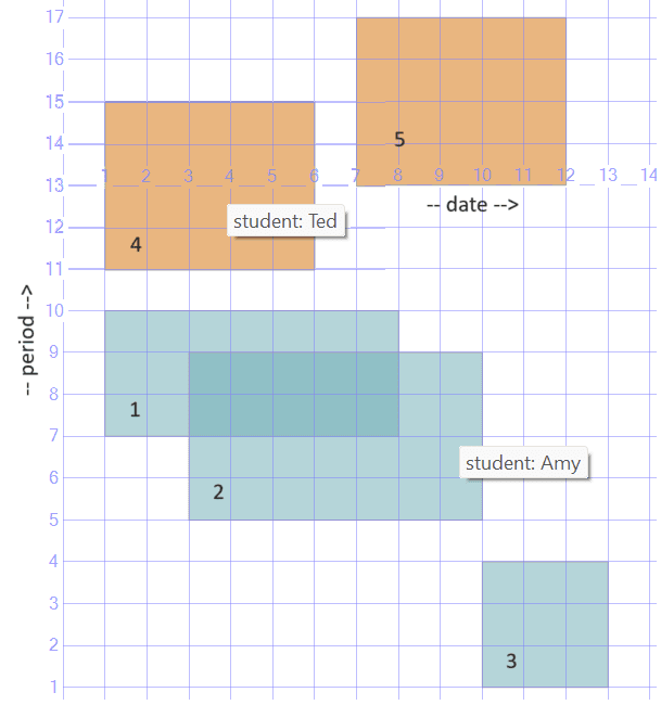
Figure 1: Unnormalized Schedule Depicted Graphically

The X axis represents the date ranges, and the Y axis represents the period ranges.

Notice that a student may have overlapping schedules, as is the case with Amy’s schedules 1 and 2. You can think of the current data as representing an unnormalized form of the schedule.

Sometimes you need to query the data to identify a schedule that contains a certain date and period. For example, the following query looks for Amy’s schedule that contains date 4 and period 8:

SELECT id, student, fromdate, todate, fromperiod, toperiod
FROM dbo.Schedule
WHERE student = 'Amy'
  AND 4 BETWEEN fromdate AND todate
  AND 8 BETWEEN fromperiod AND toperiod;

This query generates the following output, showing multiple matches:

id          student fromdate    todate      fromperiod  toperiod
----------- ------- ----------- ----------- ----------- --------
1           Amy     1           7           7           9
2           Amy     3           9           5           8

Multiple matches for a single (date, period) point are only possible due to the unnormalized nature of the schedule. The challenge is to create a normalized state of the schedule, with distinct, nonoverlapping date range and period range combinations. Assuming such a normalized state is stored in a table, you then have a guarantee for no more than one matching row per input (date, period) point.

The tricky part is that there may be multiple arrangements that can achieve this goal. For the sake of this challenge, you just need to pick one that produces a deterministic result. For example, form a result row for each consecutive range of dates with the same period range. Figure 2 has a graphical depiction of the desired normalized schedule.

Figure 2: Desired Normalized Schedule

Informally, you’re forming the smallest number of rectangles possible using only vertical cuts. Obviously, you could go for a strategy that uses horizontal cuts. Or even something more sophisticated that uses a combination of vertical and horizontal cuts. Anyway, assuming the vertical-cuts approach, following is the desired output of your solution:

student fromdate    todate      fromperiod  toperiod
------- ----------- ----------- ----------- -----------
Amy     1           2           7           9
Amy     3           7           5           9
Amy     8           9           5           8
Amy     10          12          1           3
Ted     1           5           11          14
Ted     7           11          13          16

Told you it’s a formidable challenge. Now, to work!

Unpack/Pack Solution for One Dimensional Packing

My approach to solving the two-dimensional packing problem is to rely on a classic technique for handling one-dimensional packing, which you can think of as the Unpack/Pack technique, in multiple steps of the solution. So first, let me describe the Unpack/Pack technique for one-dimensional packing.

Suppose that in our Schedule table you only had period ranges and needed to normalize them. This is of course a completely contrived example, but I’m using it for convenience since we already have sample data available to work with. Here’s a query showing just the periods:

SELECT id, student, fromperiod, toperiod
FROM dbo.Schedule
ORDER BY student, fromperiod, toperiod;

This query generates the following output:

id          student fromperiod  toperiod
----------- ------- ----------- -----------
3           Amy     1           3
2           Amy     5           8
1           Amy     7           9
4           Ted     11          14
5           Ted     13          16

Suppose that the task was to pack intersecting periods per student. Here’s the desired output of the solution with the packed periods:

student fromperiod  toperiod
------- ----------- -----------
Amy     1           3
Amy     5           9
Ted     11          16

As mentioned earlier, there are many solutions out there for packing intervals. The Unpack/Pack solution involves the following steps:

  1. Unpack each interval to the individual values that constitute the set.
  2. Compute a group identifier using a classic islands technique.
  3. Group the data by the group identifier to form the packed intervals.

Let’s start with Step 1. You’re supposed to unpack each interval to the individual values that constitute the interval set. Recall that an interval is the set of all values between the low and high values representing the interval delimiters. For example, given that our sample data uses an integer type for the period delimiters, Amy’s interval with fromperiod 5 and toperiod 8 should be unpacked to the set {5, 6, 7, 8}.

If you’re using Azure SQL or SQL Server 2022 or above, you can achieve this with the GENERATE_SERIES function, like so:

SELECT S.id, S.student, P.value AS p
FROM dbo.Schedule AS S
  CROSS APPLY GENERATE_SERIES(S.fromperiod, S.toperiod) AS P
ORDER BY S.student, p, S.id;

This query generates the following output:

id          student p
----------- ------- -----------
3           Amy     1
3           Amy     2
3           Amy     3
2           Amy     5
2           Amy     6
1           Amy     7
2           Amy     7
1           Amy     8
2           Amy     8
1           Amy     9
4           Ted     11
4           Ted     12
4           Ted     13
5           Ted     13
4           Ted     14
5           Ted     14
5           Ted     15
5           Ted     16

If you don’t have access to the GENERATE_SERIES function, you can either create your own, or use a numbers table.

Step 2 involves computing a unique group identifier per packed interval. Observe that each packed interval contains a consecutive range of unpacked p values, possibly with duplicates. As an example, see Amy’s range between 5 and 9: {5, 6, 7, 7, 8, 8, 9}. The group identifier can be computed as the p value, minus the dense rank value (because there may be duplicates) based on p value ordering, within the student partition. Here’s the query that achieves this, showing also the dense rank values separately for clarity:

SELECT S.id, S.student, P.value AS p,
  DENSE_RANK() OVER(PARTITION BY S.student ORDER BY P.value) 
                                                     AS drk,
  P.value - DENSE_RANK() OVER(PARTITION BY S.student 
                              ORDER BY P.value) AS grp_p
FROM dbo.Schedule AS S
  CROSS APPLY GENERATE_SERIES(S.fromperiod, S.toperiod) AS P
ORDER BY S.student, p, S.id;

This query generates the following output:

id          student p      drk       grp_p
----------- ------- ------ --------- --------
3           Amy     1      1         0
3           Amy     2      2         0
3           Amy     3      3         0
2           Amy     5      4         1
2           Amy     6      5         1
1           Amy     7      6         1
2           Amy     7      6         1
1           Amy     8      7         1
2           Amy     8      7         1
1           Amy     9      8         1
4           Ted     11     1         10
4           Ted     12     2         10
4           Ted     13     3         10
5           Ted     13     3         10
4           Ted     14     4         10
5           Ted     14     4         10
5           Ted     15     5         10
5           Ted     16     6         10

You get a group identifier (grp_p) that is the same per packed interval group and unique per group.

Step 3 then groups the unpacked data by the student and the group identifier, and computes the packed interval delimiters with the MIN(p) an MAX(p) aggregates, like so:

WITH C AS
(
  SELECT S.id, S.student, P.value AS p,
    DENSE_RANK() OVER(PARTITION BY S.student ORDER BY P.value) 
                                                       AS drk,
    P.value - DENSE_RANK() OVER(PARTITION BY S.student 
                                ORDER BY P.value) AS grp_p
  FROM dbo.Schedule AS S
    CROSS APPLY GENERATE_SERIES(S.fromperiod, S.toperiod) AS P
)
SELECT student, MIN(p) AS fromperiod, MAX(p) AS toperiod
FROM C
GROUP BY student, grp_p
ORDER BY student, fromperiod;

This query generates the following desired output:

student fromperiod  toperiod
------- ----------- -----------
Amy     1           3
Amy     5           9
Ted     11          16

This technique is obviously not very optimal when the sets representing the intervals can contain large numbers of members. But it works quite well for small sets and is essential for handling the two-dimensional packing challenge.

Solution for Two-Dimensional Packing

Armed with the Unpack/Pack technique, you are ready to tackle the two-dimensional packing task. The trick is to realize that you can use it multiple times in the solution—once per dimension.

In Step 1, you unpack the two-dimensional date range, period range values to the individual date (d), period (p) values. It’s probably easiest to think of this step in graphical terms, as pixelating (thanks Paul for the terminology!) the rectangles representing each student class schedule from Figure 1 shown earlier. Here’s the code to achieve this step:

SELECT S.id, S.student, D.value AS d, P.value AS p
FROM dbo.Schedule AS S
  CROSS APPLY GENERATE_SERIES(S.fromdate, S.todate) AS D
  CROSS APPLY GENERATE_SERIES(S.fromperiod, S.toperiod) AS P
ORDER BY S.student, d, p, S.id;

This query generates the following output:

id          student d           p
----------- ------- ----------- -----------
1           Amy     1           7
1           Amy     1           8
1           Amy     1           9
1           Amy     2           7
1           Amy     2           8
1           Amy     2           9
2           Amy     3           5
2           Amy     3           6
1           Amy     3           7
2           Amy     3           7
1           Amy     3           8
2           Amy     3           8
1           Amy     3           9
2           Amy     4           5
2           Amy     4           6
1           Amy     4           7
2           Amy     4           7
1           Amy     4           8
2           Amy     4           8
1           Amy     4           9
2           Amy     5           5
2           Amy     5           6
1           Amy     5           7
2           Amy     5           7
1           Amy     5           8
2           Amy     5           8
1           Amy     5           9
2           Amy     6           5
2           Amy     6           6
1           Amy     6           7
2           Amy     6           7
1           Amy     6           8
2           Amy     6           8
1           Amy     6           9
2           Amy     7           5
2           Amy     7           6
1           Amy     7           7
2           Amy     7           7
1           Amy     7           8
2           Amy     7           8
1           Amy     7           9
2           Amy     8           5
2           Amy     8           6
2           Amy     8           7
2           Amy     8           8
2           Amy     9           5
2           Amy     9           6
2           Amy     9           7
2           Amy     9           8
3           Amy     10          1
3           Amy     10          2
3           Amy     10          3
3           Amy     11          1
3           Amy     11          2
3           Amy     11          3
3           Amy     12          1
3           Amy     12          2
3           Amy     12          3
...

You can use the following helper query to depict Step 1’s result graphically:

WITH Pixels AS
(
  SELECT S.id, S.student, D.value AS d, P.value AS p
  FROM dbo.Schedule AS S
    CROSS APPLY GENERATE_SERIES(S.fromdate, S.todate) AS D
    CROSS APPLY GENERATE_SERIES(S.fromperiod, S.toperiod) AS P
)
SELECT student,
  GEOMETRY::STGeomFromText('GEOMETRYCOLLECTION('
    + STRING_AGG(CONCAT('POLYGON((', d    , ' ', p    , ',', 
                                     d    , ' ', p + 1, ',', 
                                     d + 1, ' ', p + 1, ',', 
                                     d + 1, ' ', p    , ',', 
                                     d    , ' ', p    , '))'), ',') 
    + ')', 0) AS shape
FROM Pixels
GROUP BY student;

Figure 3 has the graphical result from the Spatial results tab in SSMS.

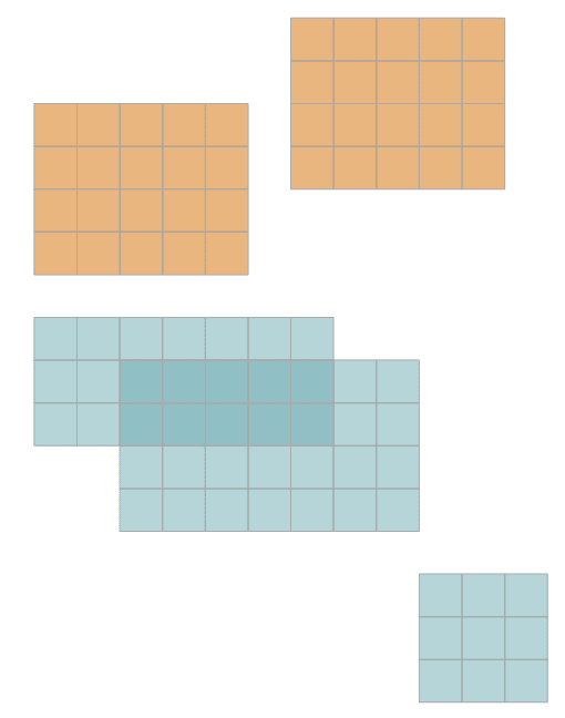
Figure 3: Pixelated Schedule

Now you need to decide on the normalization strategy that you want to use. Assuming you decide to use what I referred to earlier as the vertical cuts approach, you can proceed to Step 2. To apply vertical cuts, you pack period ranges per student and date. This is achieved by assigning the group identifier grp_p to each distinct range of consecutive p values per student and d group. Here’s the code that achieves this:

WITH PixelsAndPeriodGroupIDs AS
(
  SELECT S.id, S.student, D.value AS d, P.value AS p,
    P.value - DENSE_RANK() OVER(PARTITION BY S.student, D.value 
                                ORDER BY P.value) AS grp_p
  FROM dbo.Schedule AS S
    CROSS APPLY GENERATE_SERIES(S.fromdate, S.todate) AS D
    CROSS APPLY GENERATE_SERIES(S.fromperiod, S.toperiod) AS P
)
SELECT student, d, MIN(p) AS fromperiod, MAX(p) AS toperiod
FROM PixelsAndPeriodGroupIDs
GROUP BY student, d, grp_p
ORDER BY student, d, grp_p;

Here’s the output of the inner query defining the CTE PixelsAndPeriodGroupIDs, showing the computed grp_p value per pixel, if you will:

id          student d           p           grp_p
----------- ------- ----------- ----------- --------------------
1           Amy     1           7           6
1           Amy     1           8           6
1           Amy     1           9           6
1           Amy     2           7           6
1           Amy     2           8           6
1           Amy     2           9           6
2           Amy     3           5           4
2           Amy     3           6           4
2           Amy     3           7           4
1           Amy     3           7           4
1           Amy     3           8           4
2           Amy     3           8           4
1           Amy     3           9           4
2           Amy     4           5           4
2           Amy     4           6           4
2           Amy     4           7           4
1           Amy     4           7           4
1           Amy     4           8           4
2           Amy     4           8           4
1           Amy     4           9           4
2           Amy     5           5           4
2           Amy     5           6           4
2           Amy     5           7           4
1           Amy     5           7           4
1           Amy     5           8           4
2           Amy     5           8           4
1           Amy     5           9           4
2           Amy     6           5           4
2           Amy     6           6           4
2           Amy     6           7           4
1           Amy     6           7           4
1           Amy     6           8           4
2           Amy     6           8           4
1           Amy     6           9           4
2           Amy     7           5           4
2           Amy     7           6           4
2           Amy     7           7           4
1           Amy     7           7           4
1           Amy     7           8           4
2           Amy     7           8           4
1           Amy     7           9           4
2           Amy     8           5           4
2           Amy     8           6           4
2           Amy     8           7           4
2           Amy     8           8           4
2           Amy     9           5           4
2           Amy     9           6           4
2           Amy     9           7           4
2           Amy     9           8           4
3           Amy     10          1           0
3           Amy     10          2           0
3           Amy     10          3           0
3           Amy     11          1           0
3           Amy     11          2           0
3           Amy     11          3           0
3           Amy     12          1           0
3           Amy     12          2           0
3           Amy     12          3           0
…

And here’s the output of outer query, showing the packed period ranges after grouping:

student d           fromperiod  toperiod
------- ----------- ----------- -----------
Amy     1           7           9
Amy     2           7           9
Amy     3           5           9
Amy     4           5           9
Amy     5           5           9
Amy     6           5           9
Amy     7           5           9
Amy     8           5           8
Amy     9           5           8
Amy     10          1           3
Amy     11          1           3
Amy     12          1           3
Ted     1           11          14
Ted     2           11          14
Ted     3           11          14
Ted     4           11          14
Ted     5           11          14
Ted     7           13          16
Ted     8           13          16
Ted     9           13          16
Ted     10          13          16
Ted     11          13          16

What’s important to note here is that you created packed period ranges per student and date. This is convenient to depict graphically using the following spatial query:

WITH PixelsAndPeriodGroupIDs AS
(
  SELECT S.id, S.student, D.value AS d, P.value AS p,
    P.value - DENSE_RANK() OVER(PARTITION BY S.student, D.value 
                                ORDER BY P.value) AS grp_p
  FROM dbo.Schedule AS S
    CROSS APPLY GENERATE_SERIES(S.fromdate, S.todate) AS D
    CROSS APPLY GENERATE_SERIES(S.fromperiod, S.toperiod) AS P
),
DailyPeriodRanges AS
(
  SELECT student, d, MIN(p) AS fromperiod, MAX(p) AS toperiod
  FROM PixelsAndPeriodGroupIDs
  GROUP BY student, d, grp_p
)
SELECT student,
  GEOMETRY::STGeomFromText('GEOMETRYCOLLECTION('
    + STRING_AGG(CONCAT('POLYGON((',d,' ',fromperiod  , ',', 
                                 d,' ',toperiod + 1,',', 
                                 d + 1,' ',toperiod + 1, ',', 
                                 d + 1,' ',fromperiod ,',',
                                 d,' ',fromperiod,'))'),',') 
    + ')', 0) AS shape
FROM DailyPeriodRanges
GROUP BY student;

The output from the Spatial results tab in SSMS shown in Figure 4.

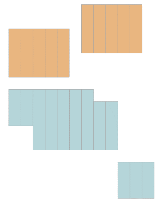
Figure 4: Daily Period Ranges

What you achieved here is sort of daily binning (again, thanks Paul for the terminology) of the packed period ranges. What’s left then in Step 3, is to pack consecutive date ranges per student and period range. Here’s the code to achieve this:

WITH PixelsAndPeriodGroupIDs AS
(
  SELECT S.id, S.student, D.value AS d, P.value AS p,
    P.value - DENSE_RANK() OVER(PARTITION BY S.student, D.value 
                                ORDER BY P.value) AS grp_p
  FROM dbo.Schedule AS S
    CROSS APPLY GENERATE_SERIES(S.fromdate, S.todate) AS D
    CROSS APPLY GENERATE_SERIES(S.fromperiod, S.toperiod) AS P
),
PeriodRangesAndDateGroupIDs AS
(
  SELECT student, d, MIN(p) AS fromperiod, MAX(p) AS toperiod,
    D - DENSE_RANK() OVER(PARTITION BY student, MIN(p), MAX(p) 
                          ORDER BY d) as grp_d
  FROM PixelsAndPeriodGroupIDs
  GROUP BY student, d, grp_p
)
SELECT student, MIN(d) AS fromdate, MAX(d) AS todate, 
       fromperiod, toperiod
FROM PeriodRangesAndDateGroupIDs
GROUP BY student, fromperiod, toperiod, grp_d
ORDER BY student, fromdate, fromperiod;

The main trick here is that in the second CTE (PeriodRangesAndDateGroupIDs), where you apply the classic islands technique a second time, when computing the dense rank value, you partition it by the student and the period range (student, MIN(p), MAX(p)), and order it by d.

Here’s the output of the second CTE’s inner query:

student d           fromperiod  toperiod    grp_d
------- ----------- ----------- ----------- ----------
Amy     10          1           3           9
Amy     11          1           3           9
Amy     12          1           3           9
Amy     8           5           8           7
Amy     9           5           8           7
Amy     3           5           9           2
Amy     4           5           9           2
Amy     5           5           9           2
Amy     6           5           9           2
Amy     7           5           9           2
Amy     1           7           9           0
Amy     2           7           9           0
Ted     1           11          14          0
Ted     2           11          14          0
Ted     3           11          14          0
Ted     4           11          14          0
Ted     5           11          14          0
Ted     7           13          16          6
Ted     8           13          16          6
Ted     9           13          16          6
Ted     10          13          16          6
Ted     11          13          16          6

And here’s the output of the outer query, showing the final desired result with the normalized schedule:

student fromdate    todate      fromperiod  toperiod
------- ----------- ----------- ----------- -----------
Amy     1           2           7           9
Amy     3           7           5           9
Amy     8           9           5           8
Amy     10          12          1           3
Ted     1           5           11          14
Ted     7           11          13          16

If you wish to illustrate the result graphically, you can use the following helper spatial query:

WITH PixelsAndPeriodGroupIDs AS
(
  SELECT S.id, S.student, D.value AS d, P.value AS p,
    P.value - DENSE_RANK() OVER(PARTITION BY S.student, D.value
                                ORDER BY P.value) AS grp_p
  FROM dbo.Schedule AS S
    CROSS APPLY GENERATE_SERIES(S.fromdate, S.todate) AS D
    CROSS APPLY GENERATE_SERIES(S.fromperiod, S.toperiod) AS P
),
PeriodRangesAndDateGroupIDs AS
(
  SELECT student, d, MIN(p) AS fromperiod, MAX(p) AS toperiod,
    d - DENSE_RANK() OVER(PARTITION BY student, MIN(p), MAX(p) 
                          ORDER BY d) as grp_d
  FROM PixelsAndPeriodGroupIDs
  GROUP BY student, d, grp_p
),
NormalizedSchedule AS
(
  SELECT student, MIN(d) AS fromdate, MAX(d) AS todate, 
        fromperiod, toperiod
  FROM PeriodRangesAndDateGroupIDs
  GROUP BY student, fromperiod, toperiod, grp_d
)
SELECT student,
  GEOMETRY::STGeomFromText('GEOMETRYCOLLECTION('
   + STRING_AGG(CONCAT('POLYGON((',fromdate,' ',fromperiod,',',
                                  fromdate,' ',toperiod+1,',',
                                  todate + 1,' ',toperiod+1,',',
                                  todate + 1,' ',fromperiod,',', 
                                  fromdate  , ' ', fromperiod  ,   
                               '))'), 
     ',') 
+ ')', 0) AS shape
FROM NormalizedSchedule
GROUP BY student;

The output in the Spatial results tab in SSMS is the same as what I’ve shown earlier in Figure 2 as the graphical depiction of the desired result.

Conclusion

Thanks again to Paul Wilcox for introducing the two-dimensional packing challenge. It’s a beautiful puzzler and I enjoyed very much working on it. I hope that’s the case for you too.

You saw how important it is to develop a toolbox of fundamental techniques, such as the classic islands technique, and based on it, the Unpack/Pack technique. Those were essential for solving this more complex challenge. You also saw how useful it can be to think of some tasks in graphical terms, and even utilize T-SQL spatial tools for this purpose.

Happy querying!


The post Two-Dimensional Interval Packing Challenge appeared first on Simple Talk.


from Simple Talk https://ift.tt/xyBsQte
via

Monday, January 1, 2024

Warehouse Load Patterns – Part 2 – Load Patterns

This continues and finishes my two-part series on warehouse load patterns. There are many methods to transfer rows between systems from a basic design perspective. This isn’t specific to any ETL tool but rather the basic patterns for moving data. The most difficult part in designing a pattern is efficiency. It has to be accurate and not adversely impact the source system, but this is all intertwined and dependent on efficiency. You only want to move the rows that have changed or been added since the previous ETL execution, deltas. This reduces the network load, the source system load (I/O, CPU, locking, etc.), the destination system load. Being efficient also improves the speed and as a direct result it increases the potential frequency for each ETL run, which has a direct impact on business value.

The pattern you select depends on many things. The previous part of the series covers generic design patterns and considerations for warehouse loads that can be applied to most of the ETL designs presented below. This section covers patterns I have used in various projects. I’m sure there are some patterns I have missed, but these cover the most used types that I have seen. These are not specific to any data engine or ETL tool, but the examples use SQL Server as a base for functionality considerations. Design considerations, columns available, administrative support, DevOps practices, reliability of systems, and cleanliness of data all come into consideration when choosing your actual ETL pattern.

Revised date

Referencing a reliable revised date is one of the easiest methods to determine which records to transfer between systems. The flow for a revised date pattern starts with a reliable revised date. When using this pattern, you will generally want to add a revised date to every table, even if it isn’t currently being targeted by an ETL process. The revised date must be set every time a record is created or modified. Each ETL process uses the revised date to determine which rows to pull from the source system. No additional changes are required on the source system, but the ETL must know the last revised date that was pulled or use a sliding window. It is up to the receiving system / ETL system to establish the correct date.