Using the DAX Calculate and Values Functions

If you should ever start reading a book on DAX, you will quickly reach a chapter on the CALCULATE function. The book will tell you that the CALCULATE function is at the heart of everything that you do in DAX and is the key to understanding the language. A delegate on one of my courses adopted the policy of starting every formula with =CALCULATE, and it’s not such a bad approach! This article explains how to use the CALCULATE function and also how to use the (almost) equally important VALUES function.

The Example Database for this Article

This article uses the same simple database as its two predecessors. This database shows sales of three toys for different cities around the world:

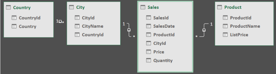
You can import this data into your own Power BI data model by first downloading this Excel workbook, or by running this SQL script in SQL Server Management Studio.

As for the previous articles in this series, everything I describe below will work just as well in Power BI, PowerPivot or Analysis Services (Tabular Model), each of which Wise Owl train.

The CALCULATE Function

To understand the CALCULATE function, you must understand filter context, so that’s where I’ll begin for this article.

Filter Context Explained Using an Excel Pivot Table

Suppose you have the following pivot table in Excel, showing the number of sales for each country, city, and product in the database. The figure selected shows that there were three sales of Timmy Tortoise products in London (UK):

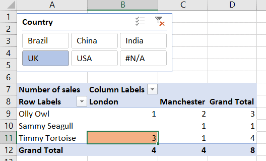
The filter context for the shaded cell containing the number 3 is therefore as follows:

Country dimension: UK

City dimension: London

Product dimension: Timmy Tortoise

If you were to double-click on this cell in Excel, you would see the underlying rows:

These are the three sales which took place for this product in this country and city.

Now suppose that you change your pivot table to show the number of sales as a percentage of the total for each column. This would give:

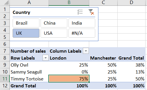
The figure for Timmy Tortoise for London is 75%, which is:

Total sales for London for Timmy Tortoise / 
Total sales for London for all products

This gives 75% because this is the result you get when you divide 3 (the number of sales in London for Timmy Tortoise) by 4 (the number of sales in London for all products).

Note that I’ll often refer in this article to the numerator and denominator. In any fraction A / B, the numerator is A and the denominator is B (but you knew that from school maths, didn’t you?).

Removing One Constraint Using CALCULATE and ALL

Now suppose that you want to recreate this pivot table using a matrix and slicer in Power BI:

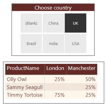
The figures are exactly the same, and for Timmy Tortoise for London you’ll see 75% because this is the ratio between the number of sales for this product and city (3) against the number of sales for all products and this city (4).

To solve this problem, you’ll use the CALCULATE function which is the answer to most questions in DAX. The syntax of the function is as follows:

The measure you should create (and show) is this:

% of all products = DIVIDE(
    // the numerator: number of sales for the current filter context
    COUNT(Sales[SalesId]),
    // the denominator: number of sales for the current filter
    // context, but for ALL products
    CALCULATE(
        COUNT(Sales[SalesId]),
        ALL('Product'[ProductName])
    )
)

I’ve put my measure in a separate table – if you’re not sure how to create this table or how to create measures, see the previous article in this series. What the measure does is to calculate the numerator (the number of sales for the current product and city) and divide this by the denominator (the number of sales for the current city only, with any product constraint removed). Here’s what this calculates:

Total sales for the current filter context / 
Total sales for the current filter context, 
but removing any product constraint

If you display row and column totals for this measure, you get this:

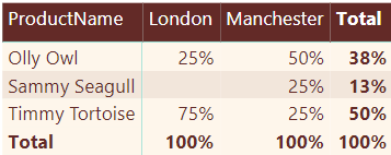
The figures in the bottom row make sense: total sales for London for all products divided by total sales for London for all products will always give 100%!

Removing Multiple Constraints Using ALL

Suppose that you now want to display the number of sales as a percentage of the total for all cities and for all products, to get this:

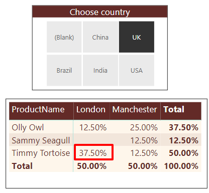
In this case, the numerator is the total number of sales in the UK in London for Timmy Tortoise, and the denominator is the total number of sales in the UK; the other two constraints have been removed from the denominator. Here is a DAX measure to calculate these figures:

% of all products and cities = DIVIDE(
    // divide the number of sales ...
    COUNT(Sales[SalesId]),
    // ... by the number of sales for all products and
    // cities
    CALCULATE(
        COUNT(Sales[SalesId]),
        ALL('Product'[ProductName]),
        ALL(City[CityName])
    )
)

You can use the ALL function as many times as you like – each time it will remove one dimension from the filter context.

Using ALLEXCEPT to Remove All but One Constraint

An alternative solution to the above problem would be to calculate this ratio:

Total sales for the current filter context / 
Total sales for the current filter context, 
but removing every constraint apart from the country one

Here’s a quick comparison of the two approaches:

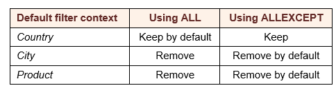
Here’s a measure which would show each product/city’s contribution to the grand total for each country:

% relaxing everything but country = DIVIDE(
    // divide the number of sales ...
    COUNT(Sales[SalesId]),
    // ... by the number of sales, keeping only the 
    // country constraint
    CALCULATE(
        COUNT(Sales[SalesId]),
        ALLEXCEPT(
            Sales,
            Country[CountryName]
        )
    )
)

It’s up to you whether you think it’s more elegant to remove constraints from the filter context individually using ALL, or to remove all constraints apart from one using ALLEXCEPT.

Replacing Filter Context Using CALCULATE

The previous examples have all involved removing the filter context in whole or in part. What if you wanted to change it to show the ratio for each matrix cell between the number of sales for that cell and the number of sales for the same filter context, but for the product Timmy Tortoise? That is, you want to calculate:

Total sales for the current filter context / 
Total sales for the current filter context, but ignoring 
any product constraint and using the Timmy Tortoise product instead

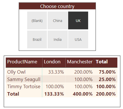
For this example, it’s inevitable that the figures for Timmy Tortoise should be 100%, because for each cell in this row you’re dividing a figure by itself. The matrix above shows that sales of Olly Owl were only a third of those for Timmy Tortoise in London but were twice those for Timmy Tortoise in Manchester.

A formula that you could use might be:

% of Timmy = DIVIDE(
    // divide the number of sales for the filter context by ...
    COUNT(Sales[SalesId]),
    // ... the number of sales for the filter context, but
    // removing any product constraint and replacing this 
    // with a constraint that the product should equal Timmy Tortoise
    CALCULATE(
        COUNT(Sales[SalesId]),
        'Product'[ProductName] = "Timmy tortoise"
    )
)

What this does is to calculate the number of sales for a particular country, city and product, and divide this by the number of sales for the same country and city, but for Timmy Tortoise. The extra filter you add in the CALCULATE formula doesn’t build on the filter context for the product, but instead replaces it.

Using the ALLSELECTED Function as Opposed to ALL

Sometimes you’ll want to reference just the selected items in a dimension, in a slicer, for example, rather than include all of the items in your formula. Here’s an example of a matrix where you might want to do this:

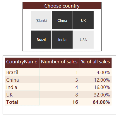
The measure shown initially is as follows:

% of all sales = DIVIDE(
    // divide number of sales for filter context ...
    COUNT(Sales[SalesId]),
    // ... number of sales for all countries
    CALCULATE(
        COUNT(Sales[SalesId]),
        ALL(Country[CountryName])
    )
)

The figures don’t add up to 100% because for each country the statistic shown equals:

the number of sales for that country / 
the number of sales for all countries

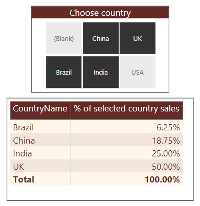
In this example the USA is included in the denominator but not in the numerator. To get the statistic to work, you need to reference only the selected countries in the denominator:

% of selected country sales = DIVIDE(
    // take the number of sales for each country
    COUNT(Sales[SalesId]),
    // divide this by the number of sales for all 
    // currently selected countries
    CALCULATE(
        COUNT(Sales[SalesId]),
        ALLSELECTED(Country[CountryName])
    )
)

This gives the required 100% total, regardless of the combination of countries you select in the slicer:

Context Transition Using the CALCULATE Function

Before moving on from the CALCULATE function, it has one more string to its bow. Consider the following two formulae:

Total sales A = SUMX(Sales,[Price]*[Quantity])
Total sales B = CALCULATE(SUMX(Sales,[Price]*[Quantity]))

If you’ve been following up to now, you’ll realise that these two formulae must give the same result under all circumstances:

The first formula gives the total sales value for the current filter context;

The second formula gives the total sales value for the current filter context, with no extra modifications to it.

However … what happens if there isn’t a filter context to begin with? In this case the second formula will create a filter context, and hence return a different answer than the first. How can you not have a filter context? By creating a calculated column in a table:

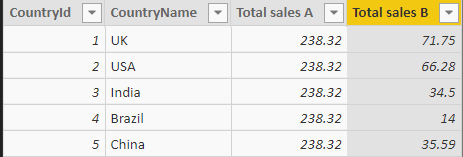
The first formula gives the same result for each row. Because calculated columns don’t have a filter context by default, the formula sums sales over all of the rows in the sales table, giving the same answer (238.32) for each.

Remember that the second formula is as follows:

Total sales B = CALCULATE(SUMX(Sales,[Price]*[Quantity]))

The CALCULATE function doesn’t just allow you to change the filter context, it can create it, too. For each country, this creates a filter context, limiting the rows in the sales table to those for the country in question, and hence giving a different answer for each row of the above table. The process of changing row context into filter context in this way is called context transition.

The VALUES Function

Learning the CALCULATE function is key to understanding how to create measures in DAX, but the VALUES function runs it a close second. The rest of this article shows what this function does, and how to use it to create a range of effects in your Power BI reports.

What the VALUES function returns

The VALUES function returns the table of data for the current filter context. To explain what this sentence means, here’s an example. Suppose you create this table in a Power BI report:

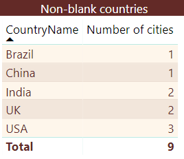
Note for this example that I’ve used a filter (not shown here) on the report to avoid showing any blank countries). The Number of cities column shows the number of cities for each country, using the following measure:

Number of cities = COUNTROWS(VALUES(City[CityName]))

If you could look at the filter context, this is what you would see:

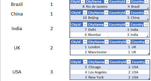
The VALUES function allows you to return a table containing one or more of the columns in the current filter context’s underlying table. For example, you could create this measure:

Cities = VALUES(City[CityName])

If you display this measure in your Power BI report, you’ll get this error message:

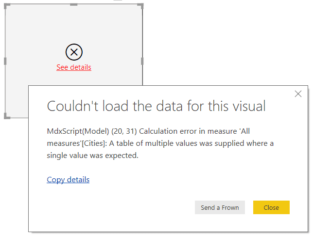
The problem is that you’re trying to display a column of values in a single cell. This would work for Brazil and China, each of which only has one city, but wouldn’t work for the other three countries.

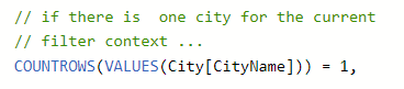
What you could do, however, is to test whether there is only one city for a country, and in this event show its name; otherwise, you could show a message saying that there are multiple cities. Here’s a measure to do this:

Cities = IF(
    // if there is  one city for the current 
    // filter context ...
    COUNTROWS(VALUES(City[CityName])) = 1,
    // ... shows the city's name
    VALUES(City[CityName]),
    // Otherwise, show a message
    "More than one city"
)

Displaying this measure in our report would give:

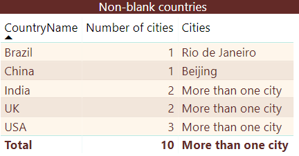
For the total row there are lots of cities in the current filter context, so naturally you get the More than one city message.

The above example shows two important features of the VALUES function. The first is that it returns a table of data. In the measure above, the COUNTROWS function expects to receive a table:

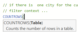
Fortunately, that’s what’s supplied:

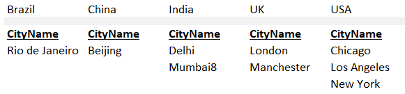
The VALUES function in this case returns a single-column table which looks like this for each of the 5 countries:

The second important point to understand about the VALUES function is that you can’t put a table into a cell without performing some sort of aggregation on it first, since a table can potentially contain multiple values. What this means is that the selected part of the measure below shouldn’t work:

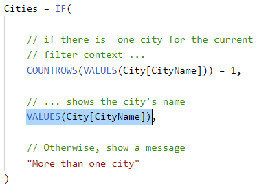
This is because the VALUES function returns a column of data, and even though you know that there is only one row in this column, and hence only one value, you would normally still need to apply some aggregation function (e.g., MAX, MIN, SUM) to the data.

Happily, there is one exception to this rule. If a call to the VALUES function returns a table with one column and one row, you can automatically treat this as a single scalar value without any additional work. This is why this measure works!

The HASONEVALUE Function and Other Alternatives

Checking whether the filter context only contains one value for a particular column is a common thing to do. It’s so common, in fact, that DAX has a dedicated function called HASONEVALUE to do this.

You could rewrite the measure like this:

Cities = IF(
    // if there is  one city for the current 
    // filter context ...
    HASONEVALUE(City[CityName]),
    // ... shows the city's name
    VALUES(City[CityName]),
    // Otherwise, show a message
    "More than one city"
)

Another solution would be to count how many distinct city names there are in the current filter context:

Cities = IF(
    // if there is  one city for the current 
    // filter context ...
    DISTINCTCOUNT(City[CityName]) = 1,
    // ... shows the city's name
    VALUES(City[CityName]),
    // Otherwise, show a message
    "More than one city"
)

These three methods, using VALUES, HASONEVALUE or DISTINCTCOUNT, are interchangeable, and I don’t think there’s any clear reason to favour one over another.

Using CONCATENATEX to List Out Multiple Values

For this example, you might want to list out the names of the cities for each country. You can do this using the CONCATENATEX function, which has this syntax:

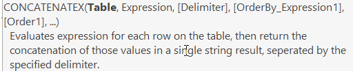
The arguments to this function are thus:

• The table containing the values you want to concatenate
• The column in this table containing the values to concatenate. You have to specify this even if the table only has one column, even though in this case it is blindingly obvious that this is the one you should choose!
• The text you want to use as glue to join the column values together
• Which column you want to order by. Again you need to specify this, even if you know you’re working with a single-column table.
• The order-by direction, ascending or descending

For this example, you could modify the measure to read like this:

Cities = IF(
    // if there is one city for the current 
    // filter context ...
    DISTINCTCOUNT(City[CityName]) = 1,
    // ... shows the city's name
    VALUES(City[CityName]),
    // Otherwise, list all city names    
    CONCATENATEX(
        VALUES(City[CityName]),
        City[CityName],
        ",",
        City[CityName],
        ASC
    )
)

This more or less works, since it gives this table:

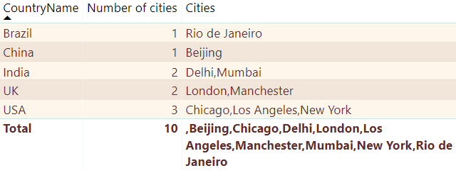
The only remaining problem is that the total row now looks odd. Technically it is correct, because, for this row, the filter context contains all of the cities for all countries. A better solution would be to check whether there is more than one country in the filter context:

Cities = IF(
    // if there's only one country in the filter context ... 
    HASONEVALUE(Country[CountryName]),
    // ... show the city name or names ...
    IF(
        // if there is  one city for the current 
        // filter context ...
        DISTINCTCOUNT(City[CityName]) = 1,
        // ... shows the city's name
        VALUES(City[CityName]),
        // Otherwise, list all city names    
        CONCATENATEX(
            VALUES(City[CityName]),
            City[CityName],
            ",",
            City[CityName],
            ASC
        )
    ),
    // ... or otherwise show nothing
    BLANK()
)

This is what you should now see when using this measure in the table:

All of this illustrates an important point about DAX measures. You can create a measure which gives sensible results for one particular visual, but can you be sure that it will give sensible results in another? Or in a totals row? Or a totals column, or grand total? You’ll often be faced with a trade-off in DAX between checking that a measure works under all possible circumstances and keeping things simple.

Modifying the Filter Context Using VALUES

Suppose that you now want to display the total sales for each country apart from the UK. The obvious way to do this is to sum total sales, but using the CALCULATE function to amend the filter context to omit the UK:

Value of sales = CALCULATE(
    // calculate total sales value
    SUMX(
        Sales,
        [Price] * [Quantity]
    ),
    // country not UK
    Country[CountryName] <> "UK"
)

This suffers from one major problem – it doesn’t work! Displaying this measure in a table would show the same value for every country:

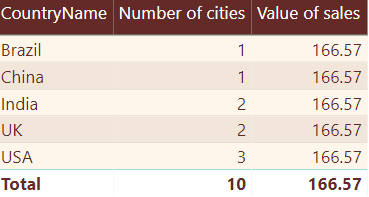
To understand why this measure is showing 166.57 for every country, remember what I said earlier in this article: when you apply a filter, it replaces the current filter context for a dimension. For this example you’re adding this filter to the CALCULATE function:

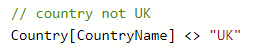
What this does is to lose any existing filter by the country dimension and replace it with one where the country is UK. Here’s what’s going on for each country:

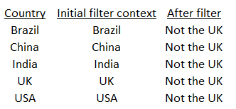
The total sales value for all of the countries apart from the UK is 166.57, so that’s what gets displayed in every row. What you want to do is to keep the existing filter context constraints for the country dimension, but then add to them. One way to do this is to use the VALUES function, making the new measure read like this:

Value of sales = CALCULATE(
    // calculate total sales value
    SUMX(
        Sales,
        [Price] * [Quantity]
    ),
    // keep the country filter as it is
    VALUES(Country[CountryName]),
    // and add that the country should not be the UK
    Country[CountryName] <> "UK"
)

This would give the following results:

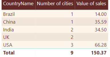
If you’re wondering why there is a discrepancy between the 166.57 shown in the first table and the 150.37 shown in the second, it’s explained by the fact that I had filtered the table to remove any sales taking place with no assigned country. If you remove this filter you get:

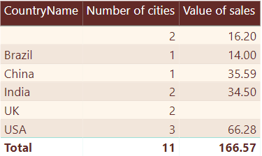
Add these 16.20 of sales in as above and you would get the required figure.

Using Disconnected Slicers to Make Reports Dynamic

This is a clever idea, which allows you to make reports dynamic. The idea is to create a slicer which allows you to choose which measure you want to show. In the example below, someone has chosen to show the average price of sales:

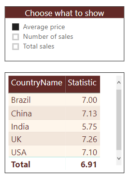
To make this work, first create a table to hold the statistics that you might want to report:

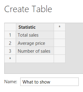
However, don’t link this table to any other. That’s why this technique is often called a “disconnected slicer”. Now create a slicer based upon this table:

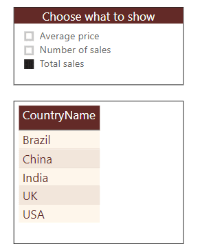
The idea is that when you select a statistic in the slicer, the bottom table will show its value. All that you now need to do is to create and show a measure which will yield:

• The average price of sales if someone selects the first measure;
• The number of sales records if someone selects the second measure;
• The total value of sales if someone selects the third measure; or
• A blank if someone selects more than one statistic at a time or doesn’t select one at all.

Here’s what this measure might look like!

Statistic = 
    // first find out what user wants to see (assume one thing chosen)
    VAR Choice = SELECTEDVALUE('What to show'[Statistic])
    // return different measure according to choice
    RETURN
        IF(
            HASONEVALUE('What to show'[Statistic]),
            SWITCH (
                Choice,
                "Average price", AVERAGE(Sales[Price]),
                "Number of sales", COUNTROWS(Sales),
                "Total sales",SUMX(Sales,[Price]*[Quantity])
            ),
            BLANK()
        )

One final question: is it possible to display different statistics using different number formatting? I can’t think of any way to do this except to use the FORMAT function:

Statistic = 
    // first find out what user wants to see (assume one thing chosen)
    VAR Choice = SELECTEDVALUE('What to show'[Statistic])
    // return different measure according to choice
    RETURN
        IF(
            HASONEVALUE('What to show'[Statistic]),
            SWITCH (
                Choice,
                "Average price", FORMAT(AVERAGE(Sales[Price]),"0.00"),
                "Number of sales", FORMAT(COUNTROWS(Sales),"#,##0"),
                "Total sales",FORMAT(SUMX(Sales,[Price]*
                                        [Quantity]),"#,##0.00")
            ),
            BLANK()
        )

The problem with this is that the FORMAT function turns numbers into text, although because it does so only after the calculation is complete for each filter context, this shouldn’t cause too much of a problem. Here’s what you’d see for the number of sales for the above measure, for example:

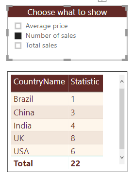
And just in case you’re wondering, I can’t think of any way to change the column title dynamically!

Dynamic Titles

There’s one more thing to demonstrate with the creative use of the VALUES function: how to show the choices made in a slicer. For the report page below, you’d like a card visual (shown selected) to display a measure listing the countries chosen:

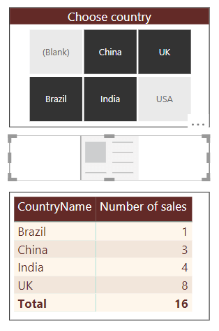
Here are some examples of what the card should display:

• For the choices shown above, it should read “Brazil, China, India, UK”
• If a user doesn’t select a country, it should read “All countries”
• If a user picks a single country, it should give the country’s name

If you’ve been following the article so far, there’s nothing new with this – it just combines lots of the ideas you’ve already seen. Here’s a measure which would fit the bill:

Title = IF(
    // if there are countries selected ...
    ISFILTERED(Country[CountryName]),
    // test to see if one, or more than one
    IF(
        HASONEVALUE(Country[CountryName]),
        // there's one country selected; show it (but must use
        // the VALUES function to convert the single column, 
        // single row table into a scalar
        VALUES(Country[CountryName]),
        // otherwise, join the country names together
        CONCATENATEX(
            Country,
            Country[CountryName],
            ",",
            Country[CountryName],
            ASC
        )
    ),
    // if we get here, then user didn't select
    // any countries
    "All countries"
)

Here’s what this would show if you have one country selected assuming that you attach the measure to your card:

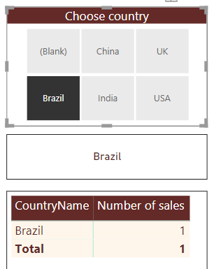
If you have multiple countries selected, you’ll see this:

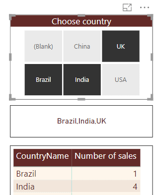
And finally, if you have no countries selected, you’ll see this:

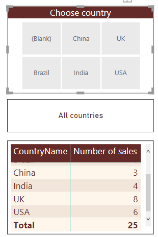
If you want to be even fancier you could use a quick measure to display only the first 3 countries in any list which I covered in the previous article in this series.

Conclusion

This article has shown how you can use two of the most important DAX functions: CALCULATE and VALUES. The article began by showing how you can use the CALCULATE function to amend the default filter context, mainly in order to create ratios. I then showed how you can use functions like VALUES, HASONEVALUE and ISFILTERED to produce a variety of clever effects in DAX. The next article in this series will look at the FILTER and EARLIER functions. You should make sure that you understand clearly how you can use the CALCULATE function to change filter context before progressing, since the DAX formulae won’t get any easier!

 

The post Using the DAX Calculate and Values Functions appeared first on Simple Talk.

from Simple Talk http://bit.ly/2RtgBjd
via

A real parameterization problem with a plus

A few weeks ago I faced this problem: One query on my application was (fortunately in the development environment) was facing a very bad execution time.

Since the query was generated by entity framework, I used SQL Profiler to capture the query with all its parameters and execute in SSMS. The query was created using sp_executesql, this stored procedure is used to force a query to be parameterized.

The surprise: The execution was quite well on SSMS. The query was the same, same server, same data, same parameters and still, the execution time was completely different. I cleared the cache many times, tried again the application, then SSMS and still, completely different execution times on both. The execution should be the same, why in hell the plan created when the application sends the query would be different than the plan created when SSMS sends the query?

Ok, the plans shouldn’t be different, but let’s check anyway. We can recover the query plans from the cache:

select * from
sys.dm_exec_query_stats qs
cross apply sys.dm_exec_sql_text(qs.sql_handle)
cross apply sys.dm_exec_query_plan(qs.plan_handle)
order by total_elapsed_time desc

 

This query will retrieve all the plans from the cache. A few more filters over the query text and we can find the plans related to the query we are looking for. Surprise again: The same query has two different plans.

How do I know it’s the same query? Couldn’t the text be different? Simple: The sql_handle was absolutely the same. It was the same query. Why different plans?

My first thought was the user. When a table name is not fully qualified (<schema>.<table>), the query plan can be fixed for a specific user and this could be a problem.

Using the query plan handles from both plans of the query and the query below we can identify if the plans are linked to a specific user or not.

with qry as
(select refcounts,usecounts,size_in_bytes, cacheobjtype,
     objtype, attribute,value,plan_handle
  from sys.dm_exec_cached_plans ecp
  outer apply sys.dm_exec_plan_attributes(ecp.plan_handle) epa
  where epa.attribute=‘user_id’)
select refcounts,usecounts,size_in_bytes,cacheobjtype,
       objtype,attribute,value, objectid,[text],[dbid]
from qry
cross apply sys.dm_exec_sql_text(qry.plan_handle)
   where dbid=db_id(<databaseName>)
          and plan_handle in (<planhandle1>,<planhandle2>)

 

No solution: both plans with a -2 value for the user_id, so both can be used by any user. Oh, wait: user_id is a plan attribute, what about the other plan attributes? We just need to remove the where clause on this previous query to check:

with qry as
(select refcounts,usecounts,size_in_bytes, cacheobjtype,
     objtype, attribute,value,plan_handle
  from sys.dm_exec_cached_plans ecp
  outer apply sys.dm_exec_plan_attributes(ecp.plan_handle) epa)
select refcounts,usecounts,size_in_bytes,cacheobjtype,
       objtype,attribute,value, objectid,[text],[dbid]
from qry
cross apply sys.dm_exec_sql_text(qry.plan_handle)
   where dbid=db_id(<databaseName>)
          and plan_handle in (<planhandle1>,<planhandle2>)

 

That’s it! Comparing all the attributes, one of them is different between both plans: set_options.

This attribute, set_options, is expressed with a numeric value which needs some bitwise operations to be parsed. Here a script to parse the set_options value, you can read it in details here

declare @set_options int = 251
if ((1 & @set_options) = 1) print ‘ANSI_PADDING’
if ((4 & @set_options) = 4) print ‘FORCEPLAN’
if ((8 & @set_options) = 8) print ‘CONCAT_NULL_YIELDS_NULL’
if ((16 & @set_options) = 16) print ‘ANSI_WARNINGS’
if ((32 & @set_options) = 32) print ‘ANSI_NULLS’
if ((64 & @set_options) = 64) print ‘QUOTED_IDENTIFIER’
if ((128 & @set_options) = 128) print ‘ANSI_NULL_DFLT_ON’
if ((256 & @set_options) = 256) print ‘ANSI_NULL_DFLT_OFF’
if ((512 & @set_options) = 512) print ‘NoBrowseTable’
if ((4096 & @set_options) = 4096) print ‘ARITH_ABORT’
if ((8192 & @set_options) = 8192) print ‘NUMERIC_ROUNDABORT’
if ((16384 & @set_options) = 16384) print ‘DATEFIRST’
if ((32768 & @set_options) = 32768) print ‘DATEFORMAT’
if ((65536 & @set_options) = 65536) print ‘LanguageID’

 

Finally, the answer: SSMS had one single option more than the connections made by the application. ARITH_ABORT changes the SQL Server behaviour when a math error, such as overflow or division by zero, happens. Should SQL Server return null or raises an error?

The option itself doesn’t affect the query in anything, however, since SSMS has a different set option enabled, SQL Server refuses to re-use the query plan created for the application and compile a new one. This totally hides the source of the problem.

After discovering the logic behind the different query plans, identifying the problem was quite easy. The query was parameterized, it was using sp_executesql. The application is a web application hosted inside sharepoint. The first time the page loads, it loads a report with only a quarter for 2018, a small set of data. However, by doing this the query is sent to the server and a query plan is stored on the cache, compiled for this set of parameters and data. When the user changes the parameters, requesting a report from 2014 to 2018, the query returns a completely different amount of data and the plan works very badly for it.

In summary, it’s a parameterization problem, when the query needs different plans for different parameter values. I wrote about the problem, how to identify and solve, you can read here. I was capturing the text and parameters of the query with problems and when executing in SSMS, due to the different set options, it was always recompiled and a new (and good) plan was created, hiding the parameterization problem.

The solution for the parameterization problem is to use a query hint. There are two options:

Recompile: This hint will ensure the query will always be recompiled, never using a plan from the cache and ensuring it always has a good plan for the current parameters.

Optimize for Unknown: The parameterization problem happens because the query is optimized for the parameter values it’s using when it first arrives on the server and this optimization may not work for other parameter values. The Optimize for Unknow hint optimize the query for any parameter value, disregarding the values used on the first execution, so it’s more probably the resulting plan will work well enough for any parameter and the query will not need to be recompiled on each execution. On the other hand, some parameters that could have a better plan will also be using this “generic” plan.

However, the query was generated by entity framework and entity framework doesn’t support query hints. How to solve this problem? Some time ago I wrote an article about how to create a library to support these query hints with entity framework. You can read the details here and get a copy of the library here.

Finally, problem solved after an interesting catch be found hiding the real problem.

The post A real parameterization problem with a plus appeared first on Simple Talk.

from Simple Talk http://bit.ly/2snYsV7
via

Empty Thoughts: Working with NULL

One of the hardest concepts in learning SQL is the meaning of a NULL. Traditionally, programming languages had no concept of missing or UNKNOWN data. The closest example that most programmers ran into was the ‘not applicable’ flags in spreadsheets, or the classic TBD flags for undetermined instructors, locations, or other things in print outs.

Dr. Codd defined a NULL as the lack of a value, so talking about NULL values is wrong. In SQL, however, we have to worry about physical storage. This means we have to know the data type of the column which is holding the NULL so the compiler can do its job. From that requirement, it logically follows that we can write CAST(NULL AS < data type>) and not just depend on automatic type conversions.

SQL is notorious for its three-value logic {TRUE, FALSE, UNKNOWN} which results from trying to compare a NULL to something, including another NULL. Since it is not a value, NULL <> NULL is UNKNOWN, but likewise so is NULL = NULL! This why we have the predicate <expression> IS [NOT] NULL to check for a NULL. This predicate and the EXISTS()function are some of the few predicates in SQL that can only return {TRUE, FALSE}.

-- Returns 'NULL IS NULL’
IF NULL IS NULL
 PRINT 'NULL IS NULL'
ELSE
 PRINT 'NULL IS NOT NULL';

NULLs in DDL

SQL defines a PRIMARY KEY(<column list>) as being implicitly declared NOT NULL. It is probably a good idea to go ahead and put the NOT NULL in your table declarations anyway. If the PRIMARY KEY constraint changes, then you are still safe. According to Dr. Codd and relational theory, to be a real table it must have a key. Originally, Dr. Codd said a PRIMARY KEY had to be designated, but later realized that a key is a key, so there’s no need to designate something special about one of them. This was another leftover from trying to implement relational systems on top of old file systems. In file systems, records (which are nothing like rows) come in a linear search sequence in physical storage, so tapes had to be sorted. The original sort key became the PRIMARY KEY in the new SQL products. Random access on unsorted magnetic tapes is technically possible, but it really doesn’t work.

But the relational model accommodates multiple keys in the same table. The syntax we picked for non- primary keys was a little strange. We added the UNIQUE(<column list>) constraint which guarantees that all the rows in the table will be different. It also allows more than one column, but the columns involved can have NULLs. Remember that in the relational model, a key can’t have NULLs, But you’re only allowed to have one NULL-ed row, as if it were a value.

All of these strange rules come from the GROUP BY clause. Without lapsing into a college algebra lesson, we have two equivalence relations, as they are called in set theory. The first is just regular old equals (=) with the extra rules about NULLs. The second relation is the GROUP BY, in which all the NULLs are put into one equivalence class.

CREATE TABLE Foobar
(foo_id CHAR(5) NOT NULL PRIMARY KEY, 
 a1 INTEGER, 
 a2 INTEGER, 
 a3 INTEGER, 
CHECK ((a1 +a2 +a3) < 10)
);
INSERT INTO Foobar VALUES ('test1', 1, 1, 1); --- works!
INSERT INTO Foobar VALUES ('test2', 10, 10, 10); --- fails!
INSERT INTO Foobar VALUES ('test3', NULL, 1, 1); --- works!

However, in the DDL, the UNKNOWN result of the search condition in a CHECK(<search condition>) constraint is given the ‘benefit of the doubt’ and treated the same as TRUE.

NULLs in DML

When you use it in the DML statements, it treats the UNKNOWN result the same as a FALSE. Query updates and inserts have a stronger criterion.

SELECT foo_id
 FROM Foobar
WHERE (a1 +a2 +a3) < 10;

returns only test1 as a result. The test2 row failed to insert. The test3 row became

“WHERE (NULL + 1 +1) < 10”

“WHERE (NULL + 2) < 10”

“WHERE NULL < 10”

“WHERE UNKNOWN” or “WHERE FALSE”

Replacing NULLs with actual values is very often handy. The SQL Server/Sybase family originally had the function ISNULL(<expression>, <non-NULL value>). If the <expression> was NULL then it returns the <value>. The data type of the result is taken from the first parameter. That particular choice can make for some funny results when parameters are not the same data types.

Microsoft now has the ANSI/ISO Standard COALESCE(<expression list>). The first thing to notice is that COALESCE takes a list of expressions, which it then parses left to right to determine the highest data type in the list, which becomes the data type of the result. The list is then parsed again from left to right to find the first non-NULL value, which is returned and cast to the result data type. One common mistake beginners make with this is to put a higher data type in the list when it’s not what they really meant.

I’m often asked why we chose the word “coalesce” instead of something else. We were trying to come up with the word that would be descriptive but not so common that it might be misunderstood or used as a column name. Phil Shaw of IBM pulled out a pocket thesaurus and started going down synonyms until he came up with this.

Grouping NULLs

A common way to use the grouping relation to return TRUE if two expressions are both NULL or their values match:

CASE WHEN 
 COALESCE(foobar, 'weird value that does not occur in the database') 
 = COALESCE(barfoo, 'weird value that does not occur in the database')
 THEN 0
 ELSE 1
 END = 0

What if there is no ‘weird value’ you can use for the COALESCE check? You just need to add more search conditions:

CASE WHEN (foo = bar OR (foo IS NULL AND bar IS NULL))
 THEN 0
 ELSE 1
 END = 0

While SQL Server does not yet have this construct, the SQL Standards added another comparison operator for this problem. This feature was introduced in two steps: SQL:1999 added T151, DISTINCT predicate. The optional negation with NOT was added by SQL:2003 as feature T152, DISTINCT predicate with negation.

<expression> IS [NOT] DISTINCT FROM <expression>

Note that you have to use the negated form to get the results you want. The un-negated form is not really equality. This is easy to see with a truth table:

A	B	A = B	A IS NOT DISTINCT FROM B
0	0	TRUE	TRUE
0	1	FALSE	FALSE
0	NULL	UNKNOWN	FALSE
NULL	NULL	UNKNOWN	TRUE

Set Operators and NULLs

SQL has set operators (UNION, INTERSECT, EXCEPT) which work on table expressions. Both tables have to be what we call ‘union compatible,’ which means the tables have the same structure (the corresponding columns in each table are in the same order and have compatible datatypes) , and the result will have that structure. Most people don’t know that technically the result table does not have a name nor do the columns unless you actually assigned them with a <set expression> AS <table name> (column name list>) construct.

Set operators discard the duplicate rows and use the grouping rather than the equality relationship to discard multiple NULLs as well as duplicate values. The EXCEPT and INTERSECT operators also work in this way.

CREATE TABLE T1 (x INTEGER);
 INSERT INTO T1 VALUES (NULL);
CREATE TABLE T2 (y INTEGER);
 INSERT INTO T2 VALUES (NULL);
-- Returns one NULL result 
 SELECT * FROM T1 
UNION 
SELECT * FROM T2;
-- Returns one NULL result 
SELECT * FROM T1 
INTERSECT 
SELECT * FROM T2;
-- Returns an empty table
SELECT * FROM T1 
EXCEPT 
SELECT * FROM T2;

OUTER JOIN and NULLs

OUTER JOINs come in three flavors (LEFT, RIGHT, FULL) and were designed to solve an actual problem. Before the SQL-99 Standard, there was no standardized syntax for them nor a Standard definition of how they would work. Sybase in SQL Server did it one way and Oracle did it another way, then there was a product from a company called Gupta Technologies LLC that let you pick which one you wanted to use. I’m going to assume that everyone knows how an outer join works. The ‘preserved table’ is the one on the left (or right or both) side of the join operator, and the unpreserved table, if any, is the one on the opposite side. Since all datatypes in SQL must be NULLable, the values that did not match the join condition in the preserved table can be padded out with NULLs. It doesn’t matter if the original columns in the preserved table were declared NOT NULL because the result of the join is technically a whole new table.

OLAP and NULLs

When OLAP (online analytical processing) databases first came in, ANSI responded by defining some basic hierarchical aggregations in ANSI/ISO Standard SQL-99. They are defined as extensions to the GROUP BY clause. The original three were GROUPING SET, ROLLUP and CUBE. The last two are defined in the standard using the GROUPING SET construct. Rollup and cube are often called ‘super groups’ because they could be defined using the regular GROUP BY and UNION operators. As expected, the NULLs form their own group. However, we now have a special function, GROUPING (<column reference>), which returns a one if the column was created by the operation or zero otherwise. Then SQL-2003 added a multicolumn version, GROUPING_ID, that constructs a binary number from the zeros and ones in the columns in the list, using an implementation defined exact numeric data type; this is handy as you think.

These constructs allow you to do what we used to call ‘control break reports’ back in the pre-SQL days. You put a sequential file in sorted order and pass it through a program that would keep running totals in accumulators (an old term that actually used to refer to a physical feature in unit record equipment). When the controls (the columns at various levels in the hierarchy) changed, the accumulators were printed out and reset. Most of the time, frankly, this was doing running totals.

This is probably easier to see with an example. Imagine we have a file that gives us a region number and the city name along with the total sales for that city. We want to get a report that shows us the totals by region, the totals by city within the regions, and finally, a grand total for all sales in the company.

SELECT region_nbr, city_name, SUM(sale_amt) AS sales_tot
 FROM Regional_Sales
GROUP BY ROLLUP (region_nbr, city_name)
ORDER BY region_nbr, city_name;

That’s assuming that there is some sample data, the output might look like this (the right-hand most column is a comment not part of the output)

 

…	…	…	comment
‘006’	‘Austin’	500.13	city within region total
‘006’	‘Dallas’	2010060.5
‘006’	‘San Antonio’	475.01
…	…	…	…
‘006’	NULL	1190902.75	region total
…	…	…
NULL	NULL	3426563.75	grand total

The general rule in SQL is not to do data formatting in the database tier. You pass the results of the database layer to a presentation layer and that layer adds the colors, labels, does any weird filters and calculations, etc. The purpose of the database tier is just raw data. However, having said that you can write something like this:

SELECT CASE WHEN GROUPING(region_nbr) =1
                           THEN ‘Region Total’ ELSE region_nbr END,
                CASE WHEN GROUPING(city_name) = 1
                            THEN ‘City Total’ ELSE ‘City Name’ END, 
               SUM(sale_amt) AS sales_tot
 FROM Regional_Sales
GROUP BY ROLLUP (region_nbr, city_name)
ORDER BY region_nbr, city_name;

Again, you are doing something that is not recommended.

Avoiding NULLs

We debated this in the early days of ANSI X3H2. Some of the early products use the regular equality for their groupings, so each NULL became its own group. This did not work out so well. The example we had in the committee was a table of traffic tickets issued in California. Quite logically, the database designer used NULL for missing auto tags; the words none, nothing, missing, etc., (in multiple languages!) had been used on prestige tags, and the way the law was written, they were perfectly legal. There was no special checkbox on the traffic tickets for a missing tag; it had to go in the space for the tag number. The huge number of missing tags made reporting impossible when they each became one row in the summary reports.

As a default, you need to assume that all your columns will be NOT NULL, then go back and decide exactly what a NULL would mean for each particular column. If your column is on a nominal or categorical scale (see this article), you can create encodings for the missing values. For example, the ISO 5218 sex codes are (‘0’ = unknown, ‘1’ = male, ‘2’ = female, ‘9’ = not applicable or lawful person). A lawful person includes things like corporations, governments, and so forth. If a column is a temporal data type, then NULL is often used as a symbol for eternity when marking the open end of (start_timestamp, end_timestamp) intervals that have not closed yet.

Using zero for numeric data elements may or may not work as a missing value token. Blanks or empty strings may or may not work as a missing value for text. Neither of these options have any built-in special characteristics that NULLs have in SQL.

Conclusion

The simple fact is that in SQL, you really can’t escape NULLs. But think of them the way you would think about any other data design decision. Is it necessary? Is it sufficient to express the nature of the model? Is it easily understood by someone who is going to have to maintain this after you’re gone?

 

The post Empty Thoughts: Working with NULL appeared first on Simple Talk.

from Simple Talk http://bit.ly/2TJCk3l
via

Better HTML5 Input Fields

HTML5 boldly came with the claim that it would offer more realistic input fields able to serve the needs of web applications. Apparently the HTML5 standards supports a long list of input types well beyond the historical short group of text, password, checkbox, radio, file, and button form input fields. The new list includes date/time specific input fields and types of input fields to accept ad hoc data such email addresses, URLs, phone numbers and plain numbers. The syntax of the INPUT element was extended to make up for new features. For example, the date input field now recognizes two extra attributes such as min and max to denote the earliest and latest dates that the control can accept.

It’s not gold all that shines though. Much of the work is left to browsers, and browsers, for a number of reasons, don’t typically hard-code much of the behavior that one might expect. In particular, no browser would check the validity of the input the user entered until the form is submitted. This means that users are apparently allowed to type any sort of characters in, say, a numeric input field just to find out that the input is invalid when they push the submit button. The same thing happens for phone numbers, websites, email addresses, dates and the like.

Finding a workaround is not a hard task, but it takes a bit of JavaScript code. Worse yet, it takes a bit of JavaScript code that must be written over and over again for every single use of any of the rich HTML5 input fields. This article intends to provide a jQuery-based JavaScript library—just a bunch of selectors actually—that when loaded into a layout page will extend a standard and more specific behavior to some HTML5 input fields. In particular, the library will automatically pre-process a number of HTML5 input fields adding to them the ability to react to invalid input on the blur event. The benefit for web developers is that you only need to reference the JavaScript library and that’s it—all will happen silently and effectively.

Although the library is provided as a jQuery extension, it wouldn’t take much to adapt jQuery selectors to plain DOM selectors and make it work even without jQuery.

Covered Use Cases

The HTML form input fields being modified in this article is described in the table below that lists the type of the input field and the implemented changes.

INPUT	DESCRIPTION
<input type=”email” />	Validate the email address as the user tabs out based on a fixed regular expression
<input type=”url” />	Validate the URL as the user tabs out based on a fixed regular expression
<input type=”tel” />	Validate the phone number based as the user tabs out based on user-defined regular expression
<input type=”number” />	Forces the user to only enter digits and automatically refuses any number outside the min/max range.
<input type=”password” />	Adds a button to toggle the type of the field between password and text allowing users to read the current password in clear.
<input type=”text” />	Honors the pattern attribute when the user tabs out of the field.

Let’s find out more and proceed case by case. Note that to exercise more control over validation phase of HTML5 forms, you might want to check out the spec of the validity browser API.

Validating Email Addresses

Certainty vanishes suddenly when it comes to validating emails. Every application, depending on the locales, may have different edge cases. HTML5 browsers do have a built-in engine to validate email addresses but, as mentioned, validation is only triggered upon form submission. If you want to have the email validated as soon as the user tabs out of the input field, then some ad hoc JavaScript is the only option left.

Here’s the skeleton of the JavaScript you want to have in place in all of your web pages with some HTML forms.

$("input[type=email]").on("blur",
    function () {
        var email = $(this).val();
        var re = / ... /;
        var success = re.test(email);
        if (success)
            $(this).removeClass("is-invalid");
        else
            $(this).addClass("is-invalid");
    });

A handler for the DOM blur event is set up for any INPUT element with the type attribute set to email. The jQuery-based body of the handler first grabs the current value of the input field and then checks it against a provided regular expression.

// YBQ FORMS
var success = re.test(email);

If the check is successful, then input field removes any is-invalid CSS class it may have. Otherwise, the input field just adds the is-invalid CSS class. Note that is-invalid is a Bootstrap 4 specific class aimed at rendering input fields with a red border to notify the invalid state. Needless to say, if you do not wish to use Bootstrap 4 to style your web page, then you’re welcome to apply any other CSS transformation to the DOM that reflects the invalid state of the element.

There’s a bit more you want to do, however, in the blur handler. First, you might want to deal with an empty or whitespace content. A blank field is valid or not? The idea here is to use the HTML5 required attribute to settle the question. If required is found, then the blank content should be parsed against the regular expression, otherwise, any further check is skipped and the content is validated.

$("input[type=email]").on("blur",
    function () {
        var email = $.trim($(this).val());
        var required = $(this).attr("required") != null;
        if (email.length === 0 && !required)
            return;

        // more code ...
});

Second, you can use the HTML5 pattern attribute to indicate a form-specific regular expression for the handler to process. If the attribute is not specified then the handler uses a built-in regular expression. Check out the source code for details.

$("input[type=email]").on("blur",
    function () {
        var email = $.trim($(this).val());
        var required = $(this).attr("required") != null;
        if (email.length === 0 && !required)
            return;
        var re = / ... /;
        var pattern = $(this).attr("pattern");
        if (pattern != null) {
            re = new RegExp($(this).attr("pattern"));
        }
        var success = re.test(email);
        
        // more code ...
});

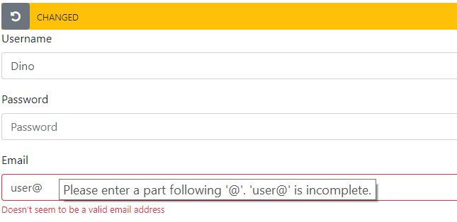
The net effect is shown in the figure below. Note that most browsers also provide detailed error messages in the form of tooltips. Note also that the error message displayed through the tooltip is based on the browser’s internal email regular expression which might be different from the one hard-coded in the library or that you may have set through the pattern attribute. To turn off the tooltip, you just set the title attribute of the INPUT field to the empty string or anything else you like.

Validating URLs

Validating a URL input field poses exactly the same challenges as validating an email address as in the HTML5 spec. The type url supports the same attributes as the type email. Here’s then the code you need to have in place.

$("input[type=url]").on("blur",
    function () {
        var url = $.trim($(this).val());
        var required = $(this).attr("required") != null;
        if (url.length === 0 && !required)
            return;
        var re = / ... /;
        var pattern = $(this).attr("pattern");
        if (pattern != null) {
            re = new RegExp($(this).attr("pattern"));
        }

        var success = re.test(url);
        if (success)
            $(this).removeClass("is-invalid");
        else
            $(this).addClass("is-invalid");
});

For details about the default regular expression used to check the scheme of the URL refer to the source code.

Validating Phone Numbers

The code to extend input fields of type tel is slightly simpler and for a good reason: there’s nearly no chance that someone can come up with a sufficiently agreed, default regular expression for validating phone numbers. Because of this, the sample library doesn’t even attempt to support a default regular expression and just uses any expressions provided through the HTML5 pattern attribute. This makes the overall blur handler a bit shorter, as below.

$("input[type=tel]").on("blur",
    function () {
        var tel = $(this).val();
        var required = $(this).attr("required") != null;
        if (tel.length === 0 && !required)
            return;
 
        var re = new RegExp($(this).attr("pattern"));
        var success = re.test(tel);
        if (success)
            $(this).removeClass("is-invalid");
        else
            $(this).addClass("is-invalid");
    });

This said, what would be at least a good candidate to validate phone numbers? Here’s my shot at it:

<div class="form-group">
    <label for="phone">Phone</label>
    <input type="tel" class="form-control" 
           id="phone" name="phone" 
   pattern="[+][0-9]{1,3} [0-9]{3}[\s-][0-9]{4}[\s-][0-9]{3}"
           placeholder="+x xxx-xxxx-xxx">
    <div class="invalid-feedback">
        Phone number must be +x xxx-xxxx-xxx
    </div>
</div>

The phone number matched by the expression above is +X XXX-XXXX-XXX. To be precise, the dash (-) can also be replaced with a blank character. The international country code is up to three digits and number is grouped in three chunks of 3, 4, 3 digits respectively.

Accepting Numbers

Personally, I just hate to be able to type anything into a textbox only to receive a warning through a tooltip and an error message later. If the input field is declared to be of type number, then users should never be able to type in anything but digits. Here’s how to do it.

$("input[type=number]")
    .on("keypress",
        function (event) {
            if (event.charCode < 48 || event.charCode > 57) {
                event.preventDefault();
                return false;
            }
        })
    .on("keyup", function () {
        var buffer = $(this).val();
        var maxLength = parseInt($(this).attr("maxlength"));
        if (buffer.length > maxLength) {
            $(this).val("");
            return false;
        }
        var minVal = parseInt($(this).attr("min"));
        var maxVal = parseInt($(this).attr("max"));
        var number = parseInt(buffer);
        if (number < minVal || number > maxVal) {
            $(this).val("");
            return false;
        }
        return true;
    });

There are two handlers: one for keypress and one for keyup. The former refuses any keyboard button different from 0-9 digits. Admittedly, this implementation doesn’t support anything but positive integers. The keyup handler, instead, ensures that any number typed falls within the defined min/max range.

HTML5, in fact, allows you to set a min and a max attribute on numeric fields to delimit the range of feasible values. However, those boundaries are not checked until the form is submitted. With the keyup implementation, instead, the current value of the buffer is turned into an integer, checked against the min/max interval and emptied if it falls outside. In this way, the input field only returns integers (or blanks) in the given range.

In addition, the keyup handler also ensures that no more digits than maxlength are ever typed. The point is that, even though the range is, say, 1-20 and no value outside 1-20 will ever be allowed when tabbing out, then there’s no reason for the user to be able to type in more than 2 digits.

Extended Password Input Fields

The HTML5 spec adds a couple of features on password input fields that alone reduce the need for validating the password at least on the client. They are minlength and maxlength attributes, whose meaning is quite self-explanatory. In addition, HTML5 password input fields also support the pattern attribute which can be set to a JavaScript acceptable regular expression. In all these cases, though, remains the issue that any validation is performed when it might be annoying for users to note—upon form submission. Here’s how to add prompt notification of min/max length violation in the proposed password.

$("input[type=password]").on("blur",
    function() {
        var pswd = $.trim($(this).val());
        var minLength = parseInt($(this).attr("minlength"));
        var maxLength = parseInt($(this).attr("maxlength"));
        if (isNaN(minLength)) {
            minLength = 0;
        }
        if (isNaN(maxLength)) {
            maxLength = 100;
        }
        if (pswd.length < minLength || 
            pswd.length > maxLength)
            $(this).addClass("is-invalid");
        else
            $(this).removeClass("is-invalid");
    });

Quite simply, the blur handler captures the value of the minlength and maxlength attributes, turns them into numbers and compares with the actual length of the password buffer. Leading and trailing blanks are automatically removed. The password field also supports a pattern attribute for you to add some regular expressions to parse the proposed password. To add support for the pattern, just copy the same code seen above for email and URL fields.

One more thing you can do for password fields is adding—automatically—a button to switch between the password and text mode so that the password can be seen in clear.

The necessary code is shown below. You just add it to the input field reference side by side with the blur handler.

$("input[type=password]").each(function() {
    $(this)
        .add(
            "<span class='input-group-btn'>" +
            "<button type='button' class='btn btn-primary' 
             onclick='__togglePswdView(this)'>" +
            "<i class='fa fa-eye'></i></button></span>")
        .wrapAll("<div class='input-group' />");
}).on("blur", function() {
    // blur handler body
});

The code just uses the Bootstrap 4 markup for input button groups and attached some plain JavaScript code to toggle the value of the password’s type attribute.

function __togglePswdView(elem) {
    var pswd = $(elem).closest("div").find("input");
    var type = $(pswd).attr("type");
    if (type === "password")
        pswd.attr("type", "text");
    else
        pswd.attr("type", "password");
}

Controlling Input in Text Fields

Sometimes input fields are only allowed to take digits, letters and perhaps a few extra chars. You can use the pattern attribute set to a regular expression but if you do so you also need some of the aforementioned JavaScript to force the expression to be matched during the blur event.

$("input[type=text]").on("blur",
    function () {
        var text = $(this).val();
        var re = /(?:)/;
        var pattern = $(this).attr("pattern");
        if (pattern != null) {
            re = new RegExp($(this).attr("pattern"));
        }
        var success = re.test(text);
        if (success)
            $(this).removeClass("is-invalid");
        else
            $(this).addClass("is-invalid");
    });

In this way, to force an alphanumeric input, you only need the following regular expression.

<input type="text" class="form-control" 
       id="username" name="username"
       pattern="[a-zA-Z0-9]" />

Summary

HTML5 is now widely supported across modern browsers, but it pays for the goal of being a broad specification. As far as INPUT fields are concerned, there are plenty of options and a good enough range of attributes. The only problem is when those attributes are honored. Validation always takes place when the form is submitted, but this is not ideal for most scenarios when you want to give users immediate feedback about what they may have been doing wrong. In this case, JavaScript is necessary and the Ybq free library that comes with this article makes it trivially easy to trigger validation when and how you most need it. The source code is available here.

 

The post Better HTML5 Input Fields appeared first on Simple Talk.

from Simple Talk http://bit.ly/2VJ0Lzt
via

SQL naming conventions

SQL naming conventions for tables, and all the associated objects such as indexes, constraints, keys and triggers, are important for teamwork. Poorly-named tables and other objects make it difficult to maintain databases.

Table names must follow the rules for SQL Server identifiers, and be less than 128 characters. It is possible to force SQL Server to accept non-standard table names by surrounding them with square brackets but it is a very bad idea, because they have to be ‘quoted’ whenever they are used in scripts.

Temporary table names are slightly different in that they are prefixed with a single number sign (#) and are limited in length to 116 characters. After any prefix with a special meaning (‘@’ meaning a table variable, ‘#’ meaning a temporary table or ‘##’ meaning a global temporary table), the first letter must be a letter as defined by Unicode Standard 3.2. This means that it is either a Latin character from A through Z, upper or lower case, or else a letter character from other languages. Subsequent characters can legally be

• Letters as defined in the Unicode Standard 3.2.,
• Decimal numbers from either Basic Latin or other national scripts,
• The ‘at sign’(@) , the ‘dollar sign’ ($), the ‘number’ or ‘hash sign’ (#)
• The underscore, normally used to represent spaces such as Overdue_Account.

Never use spaces, embedded characters or reserved names, because they aren’t portable, require square brackets, and can confuse scripts and procedures.

We can test for compliance with SQL Server identifier spec very simply with the following SQL.

SELECT name FROM sys.objects 
   WHERE name LIKE '%[^_A-Z0-9@$#]%' COLLATE Latin1_General_CI_AI
 --contains illegal characters
   OR name NOT LIKE '[A-Z]%' COLLATE Latin1_General_CI_AI
 --doesn't start with a character

We can check for reserved words in objects in this slightly bulky but efficient code

SELECT name
  FROM sys.objects
    INNER JOIN
      (
      VALUES ('ADD'), ('EXTERNAL'), ('PROCEDURE'), ('ALL'), ('FETCH'),
        ('PUBLIC'), ('ALTER'), ('FILE'), ('RAISERROR'), ('AND'),
        ('FILLFACTOR'), ('READ'), ('ANY'), ('FOR'), ('READTEXT'), ('AS'),
        ('FOREIGN'), ('RECONFIGURE'), ('ASC'), ('FREETEXT'), ('REFERENCES'),
        ('AUTHORIZATION'), ('FREETEXTTABLE'), ('REPLICATION'), ('BACKUP'),
        ('FROM'), ('RESTORE'), ('BEGIN'), ('FULL'), ('RESTRICT'), ('BETWEEN'),
        ('FUNCTION'), ('RETURN'), ('BREAK'), ('GOTO'), ('REVERT'), ('BROWSE'),
        ('GRANT'), ('REVOKE'), ('BULK'), ('GROUP'), ('RIGHT'), ('BY'),
        ('HAVING'), ('ROLLBACK'), ('CASCADE'), ('HOLDLOCK'), ('ROWCOUNT'),
        ('CASE'), ('IDENTITY'), ('ROWGUIDCOL'), ('CHECK'), ('IDENTITY_INSERT'),
        ('RULE'), ('CHECKPOINT'), ('IDENTITYCOL'), ('SAVE'), ('CLOSE'), ('IF'),
        ('SCHEMA'), ('CLUSTERED'), ('IN'), ('SECURITYAUDIT'), ('COALESCE'),
        ('INDEX'), ('SELECT'), ('COLLATE'), ('INNER'),
        ('SEMANTICKEYPHRASETABLE'), ('COLUMN'), ('INSERT'),
        ('SEMANTICSIMILARITYDETAILSTABLE'), ('COMMIT'), ('INTERSECT'),
        ('SEMANTICSIMILARITYTABLE'), ('COMPUTE'), ('INTO'), ('SESSION_USER'),
        ('CONSTRAINT'), ('IS'), ('SET'), ('CONTAINS'), ('JOIN'), ('SETUSER'),
        ('CONTAINSTABLE'), ('KEY'), ('SHUTDOWN'), ('CONTINUE'), ('KILL'),
        ('SOME'), ('CONVERT'), ('LEFT'), ('STATISTICS'), ('CREATE'), ('LIKE'),
        ('SYSTEM_USER'), ('CROSS'), ('LINENO'), ('TABLE'), ('CURRENT'),
        ('LOAD'), ('TABLESAMPLE'), ('CURRENT_DATE'), ('MERGE'), ('TEXTSIZE'),
        ('CURRENT_TIME'), ('NATIONAL'), ('THEN'), ('CURRENT_TIMESTAMP'),
        ('NOCHECK'), ('TO'), ('CURRENT_USER'), ('NONCLUSTERED'), ('TOP'),
        ('CURSOR'), ('NOT'), ('TRAN'), ('DATABASE'), ('NULL'), ('TRANSACTION'),
        ('DBCC'), ('NULLIF'), ('TRIGGER'), ('DEALLOCATE'), ('OF'),
        ('TRUNCATE'), ('DECLARE'), ('OFF'), ('TRY_CONVERT'), ('DEFAULT'),
        ('OFFSETS'), ('TSEQUAL'), ('DELETE'), ('ON'), ('UNION'), ('DENY'),
        ('OPEN'), ('UNIQUE'), ('DESC'), ('OPENDATASOURCE'), ('UNPIVOT'),
        ('DISK'), ('OPENQUERY'), ('UPDATE'), ('DISTINCT'), ('OPENROWSET'),
        ('UPDATETEXT'), ('DISTRIBUTED'), ('OPENXML'), ('USE'), ('DOUBLE'),
        ('OPTION'), ('USER'), ('DROP'), ('OR'), ('VALUES'), ('DUMP'),
        ('ORDER'), ('VARYING'), ('ELSE'), ('OUTER'), ('VIEW'), ('END'),
        ('OVER'), ('WAITFOR'), ('ERRLVL'), ('PERCENT'), ('WHEN'), ('ESCAPE'),
        ('PIVOT'), ('WHERE'), ('EXCEPT'), ('PLAN'), ('WHILE'), ('EXEC'),
        ('PRECISION'), ('WITH'), ('EXECUTE'), ('PRIMARY'), ('WITHIN GROUP'),
        ('EXISTS'), ('PRINT'), ('WRITETEXT'), ('EXIT'), ('PROC')
      ) AS reserved (word)
      ON reserved.word = sys.objects.name;

 

Beware of numbers in any object names, especially table names. It normally flags up clumsy denormalization where data is embedded in the name, as in ‘Year2017’, ‘Year2018’ etc. Usually the significance of the numbers is obvious to the perpetrator, but not to the maintainers of the system.

SELECT name FROM sys.tables
   WHERE name LIKE '%[0-9]%' COLLATE Latin1_General_CI_AI --contains numbers

If you are more relaxed about this and will tolerate single numbers but no more, then tyy this

SELECT name FROM sys.tables
   WHERE name LIKE '%[0-9][0-9]%' COLLATE Latin1_General_CI_AI 
–contains more than one adjacent number

There are no generally accepted standards for naming SQL objects. Although ISO/IEC 11179 has been referred to as a standard for naming, it actually only sets a standard for defining naming conventions. There is a sample standard in the ‘Naming principles’ document (ISO/IEC 11179-5), but this is merely an example of how a standard should be defined. However, it is quite close to a general good-practice in programming.

When naming a table, it is a good idea to use a collective name or ‘object class term’ for the entity if one exists ( such as Employee, Cost, Tree, component, member, audience, staff or faculty) but use the singular rather than the plural form where possible. For the sake of maintenance, use a consistent naming convention that is informative but brief. It helps greatly to start with a dictionary of the correct nouns and verbs associated with the application domain and use that. If it proves inadequate, then the team can build on it. If a data model has been created as part of the design phase, this dictionary should be an end-product of this work.

Never use a descriptive prefix such as tbl_. This ‘reverse-Hungarian’ notation has never been a standard for SQL and clashes with SQL Server’s naming conventions. Some system procedures and functions were given prefixes “sp_”, “xp_” or “dt_” to signify that they were ‘special’ and should be searched for in the master database first. The use of the tbl_prefix for a table, often called ‘tibbling’, came from databases imported from Access when SQL Server was first introduced. Unfortunately, this was an access convention inherited from Visual Basic, a loosely typed language. Even if prefixes were a good thing, one wouldn’t use “Tbl_” for a table. There are established codes for SQL Server and the code for a table is U (short for ‘User Table’ evidently). There are still many DBAs that long to ‘tibble’, but there is never a doubt what type of object something is in SQL Server if you know its name, schema and database, because its type is there in sys.objects: Also it is obvious from the usage. SQL Server is a strongly-typed language.

SELECT name FROM sys.objects 
  WHERE Left(name,3) IN ('tbl','sp_','xp_','dt_')  --tibbling!

Do not give a table the same name as one of its columns.

SELECT Thetable.Name FROM sys.columns cols
INNER JOIN sys.tables Thetable 
  ON Thetable.object_id = cols.object_id
  WHERE cols.NAME=Thetable.name

Avoid, where possible, concatenating two table names together to create the name of a relationship table when there is already a word in the language to describe the relationship. e.g. use Client rather than EmployeeCustomer

This code will find these tables. Don’t try it on a huge database!

SELECT name
  FROM sys.tables AS TheTable
    INNER JOIN
      (
      SELECT first.name + second.name
        FROM sys.tables AS first
          CROSS JOIN
            (SELECT name FROM sys.tables) AS second
      ) AS combined(doubleName)
      ON combined.doubleName = TheTable.name;

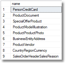
On AdventureWorks2016, you will get a few tables that could be better-named

Keep table names short, because many naming conventions require that triggers, constraints and indexes include the name of the table or tables involved. A foreign key constraint can get cumbersome

Be consistent in the casing of tables and the use of underscore for delimiting words.

A table column should be a ‘quality common to all members of an object class’ and should have a name that corresponds to the way that plain language refers to the property such as First_Name, Amount, Measure, Number, Quantity or Text. Never apply the collective name to the property, such as having an ‘Employee_name’ property in an Employee table. This would provide redundancy when the qualified column was listed in a query – Employee.Employee_name.

You can quickly find all the columns with redundancy in their names if they are expressed with the dotted notation.

SELECT TheTable.name AS TableName, TheColumn.name AS ColumnName
  FROM sys.tables AS TheTable
    INNER JOIN sys.columns AS TheColumn
      ON TheColumn.object_id = TheTable.object_id
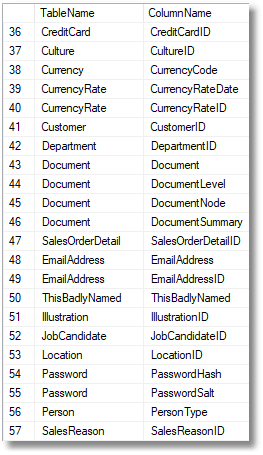
  WHERE TheColumn.name LIKE '%' + TheTable.name + '%';

AdventureWorks is full of this sort of problem.

Whoever thought up the name Person.Person.personType was short on vocabulary. It might be an idea to detect for the even more heinous crime of naming a table the same as a schema!

SELECT name FROM sys.objects WHERE Object_Schema_Name(object_id) = name;

A simple guide to naming is to respect the idea of SQL being an intelligible language based on written language. This would suggest that function names should fit into the semantics of the SELECT sentence, if we have a function that capitalises a sentence, makes the first character of each word longer than three characters a capital letter (MLA), then you’d call it ‘capitalized()’. Procedures would be verb-noun names of tasks, since they are executed.

Procedures should follow the Verb-noun convention popularised by PowerShell. Obviously, the standard verbs and nouns will come from the database design process and the data model of the organisation or the application domain.

Summary

There are certain style rules in SQL Server, but not that many. It is more important to be consistent and, where possible, write in a way that is closest to standard SQL. SQL Server gives you quite a bit of latitude in your style, but because you can do such things as putting numbers, whitespace and control characters into names doesn’t mean that you should. You can write in eccentric archaic dialects of SQL, but you are still being eccentric. In teamwork, it is best to adopt the defined standard that is in place, however absurd it may be, and work away at convincing the rest of the team to change.

SQL is unlike any other computer language in that it was designed to be as close to human language as possible, so it could be used by lay people to do business analysis. I believe that naming conventions should fit in with this basic idea so that database code reads clearly with just the minimum of documentation to assist in understanding.

See SQL Code Smells for more SQL Smells. See SQL Server Table Smells for SQL Code that flushes out more general problems with tables

The post SQL naming conventions appeared first on Simple Talk.

from Simple Talk http://bit.ly/2QxxNPu
via

The Case for Value-Based Delivery

In the past, I was very proud that I’d meticulously defended my projects against scope creep, but I was missing the point. The real reason organizations should undertake projects is to achieve value.

What should be the priority, then, defending against scope creep or value-based delivery? The agile movement fundamentally understands this. Its core principles acknowledge that requirements will change as understanding grows. However, if you look at traditional agile tools and concepts—like the burn up (or burn down) chart and the cone of uncertainty— you’ll see they are often scope-oriented.

The most important question project managers should ask themselves about any project is not “What?” but “Why?” The business case for project execution could be reducing OPEX costs or meeting compliance goals, for example. When you understand the outcome your organization or client is seeking, you will know where to direct your team and efforts.

We recently worked on a project to develop a system for a legacy customer. They did not have a system for efficiently managing interactions with the international healthcare community (healthcare professionals, patient organizations, etc.). Considering the scope of the project, it was easy to plan and deliver, but we later realized that the project had gone over budget and was extended by a couple of months. This was because of continuous growth in the project’s scope.                         

Was this a failure? I could have defended all scope changes. After the delay and going over budget, we delivered the project. The new system drove the customer’s commercial business as well as contributing to the discovery and progress of Research and Development. The customer is highly regulated and at high risk in life sciences. We were able to deliver standardized processes across international customers, provided transparency of professional’s use, and enabled compliance monitoring for risk mitigation.

Defining and reporting against these additional requirements was far more challenging than simply relying on scope, time and cost but gave us much more confidence that we were delivering business value. This approach requires very rigorous thinking and a real understanding of what it takes to deliver success. In my experience, the ability to help define the drivers of success is one of the skills that makes a project manager a great business partner.

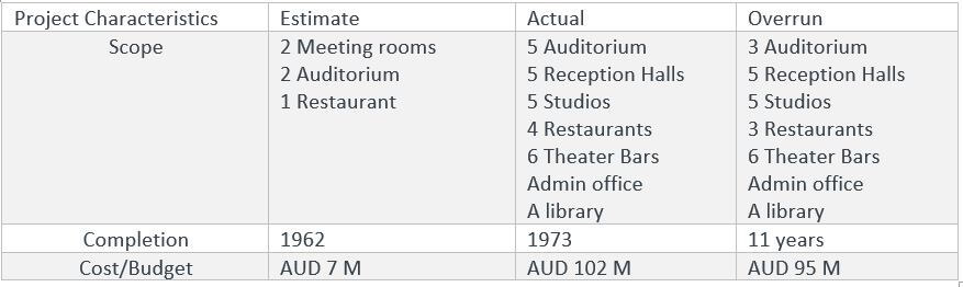
As another example, the Sydney Opera House could probably be seen as one of the most disastrous construction projects in history. The project was originally scheduled for four years, with a budget of AUS $7 million. It ended up taking 14 years to be completed at a cost of AUS $102 million. Do you see this as a failure?

Below are the project statistics which are available in public forums:

As a project, it was a failure, but as an idea, it was a huge success. It’s one of the 20th century’s most magnificent buildings and one of the 21st century’s busiest performing arts centers.

Commentary Competition

Enjoyed the topic? Have a relevant anecdote? Disagree with the author? Leave your two cents on this post in the comments below, and our favourite response will win a $50 Amazon gift card. The competition closes two weeks from the date of publication, and the winner will be announced in the next Simple Talk newsletter.

The post The Case for Value-Based Delivery appeared first on Simple Talk.

from Simple Talk http://bit.ly/2TAl1kX
via

Policy-based Authorization in ASP.NET Core – A Deep Dive

Take advantage of Policy-based authorization, a simple, rich, expressive and reusable authorization model, to secure your applications written in ASP.NET Core

Authentication and Authorization are two terms you would often come across when reading about the security of web applications. While the former is used to validate a user’s credentials, the latter is used to grant access to one or more resources of the application to a user. There are two ways in which you can implement authorization in ASP.NET Core. These include role-based authorization and policy-based authorization. Role-based authorization has been in use from the previous versions of ASP.NET. Policy-based authorization has been newly introduced in ASP.NET Core and provides a rich, expressive and reusable authorization model to secure applications developed in ASP.NET Core. This article presents a discussion on how you can work with policy-based authorization in ASP.NET Core.

Prerequisites

To work with the code examples provided in this article, you should have Visual Studio 2017 and NET. Core installed in your system. If you don’t have .NET Core installed in your system, you can download a copy from here. You can download Visual Studio 2017 from this link.

Before the deep dive into how the policy-based authorization model works, here’s a quick tour of the role-based security model to understand the constraints of the role-based security model and then learn why the policy-based authorization model should be used.

Role-based Authorization in ASP.NET Core

A role is a string value that is mapped to a set of permissions for an authenticated user. The role-based security model has been in use from the days of ASP.NET. Role-based authorization is a declarative way to restrict access to resources. You can specify the roles that the current user must be a member of to access a specified resource. The Authorize attribute enables you to restrict access to resources based on roles. It is a declarative attribute that can be applied to a controller or an action method. If you specify this attribute without any arguments, it only checks if the user is authenticated. Here’s an example that illustrates how this attribute can be applied to a controller.

using Microsoft.AspNetCore.Authorization;
using Microsoft.AspNetCore.Mvc;
[Authorize]
public class UserController : Controller
{
  //Action methods
}

The following code snippet can be used to limit access to the SecurityController to only those users who are administrators, i.e., those users who are a member of the Administrator role.

[Authorize(Roles = "Administrator")]
public class SecurityController : Controller
{
  //Usual code
}

Multiple Roles

You can also specify multiple roles, separated by a comma. Here’s an example that illustrates this.

[Authorize(Roles = "Manager,Administrator")]
public class DocumentsController : Controller
{
   //Action methods
}

In this example, only those users who pertain to the Manager or Administrator role can have access to the DocumentsController and all its methods.

Note that you can apply roles both at the controller and the action levels. As an example, even if users having either Manager or Administrator roles can access the DocumentsController and its methods, you may want a method of this controller class to be accessed only by users who belong to the Administrator role. The following code snippet shows how this can be achieved.

[Authorize(Roles = "Manager, Administrator")]
public class DocumentsController : Controller
{
    public ActionResult ViewDocument()
    {
        //Your code here
    }
    [Authorize(Roles = "Administrator")]
    public ActionResult DeleteAllDocuments()
    {
        //Your code here
    }
}

Now, suppose you would want users who belong to both Manager and Administrator roles should only have access to the DocumentsController and its methods. The following code snippet shows how you can define roles in such a way that the users who access the DocumentsController and its methods must be a member of both Manager and Administrator roles.

[Authorize(Roles = "Manager")]
[Authorize(Roles = "Administrator")]
public class DocumentsController  : Controller
{
}

Albeit its ease of use, role-based authorization has its limitations. This is exactly why policy-based authorization is used. In the sections that follow you will examine how you can work with policy-based authorization in ASP.NET Core.

The Need for Policy-based Authorization

Authorization and access control using roles for protecting resources from unauthorized access have been in use for quite some time. However, they aren’t very expressive, and you may run into problems when the number of roles that are needed is significantly high.

Here’s a scenario with an example to explain. Suppose you are tasked with designing a security framework for an application. Initially, there are three roles in an application, i.e., User, Admin, and Manager. Now if you have multiple variations of the Admin role, like, CustomerAdmin, ReportsAdmin, and SuperAdmin, you would have to consider each of these when you are designing the security framework. You can also have multiple variations of the Manager role – your framework will have to consider these as well. As the number of these roles increases significantly, it becomes extremely difficult to effectively handle the roles. Here’s exactly where a policy-based authorization model comes in.

Working with Policy-based Authorization in ASP.NET Core

A policy-based security model decouples authorization and application logic and provides a flexible, reusable and extensible security model in ASP.NET Core. The policy-based security model is centered on three main concepts. These include policies, requirements, and handlers. A policy is comprised of several requirements. A requirement, in turn, contains data parameters to validate the user’s identity. Lastly, a handler is used to determine if a user has access to a specific resource. We’ll discuss each of these in more detail in this section – we’ll start with a policy.

Essentially, a policy is comprised of one or more requirements and is usually registered at application startup in the ConfigureServices() method of the Startup.cs file. To apply the policies in your controllers or action methods, you can take advantage of the AuthorizeAttribute attribute or the AuthorizeFilter filter.

You can create a policy instance using the AuthorizationPolicyBuilder class as shown in the code snippet given below. You can specify the role names using the RequireRole method.

var policy = new AuthorizationPolicyBuilder()
  .RequireAuthenticatedUser()
  .RequireRole("Admin")
  .Build();

Alternatively, you can create the policy instance in the ConfigureServices method as shown in the code snippet given below.

services.AddMvc(obj =>
            {
                var policy = new AuthorizationPolicyBuilder()
                    .RequireAuthenticatedUser()
                    .Build();
                obj.Filters.Add(new AuthorizeFilter(policy));
            });

You’ll see more on this in the sections that follow.

Registering a Policy

Merely defining the policies isn’t enough – you should also register the policies you’ve defined with the authorization middleware. To register a policy, you should specify a name – this name would be used to reference the policy in the controller or the action methods.

The following code snippet illustrates how a policy can be registered at application startup in ASP.NET Core.

using Microsoft.Extensions.DependencyInjection;
public void ConfigureServices(IServiceCollection services)
{
    services.AddMvc();
    services.AddAuthorization(options =>
    {
        options.AddPolicy("RequireManagerOnly", policy => 
               policy.RequireRole("Manager"));
    });
}

You can also specify multiple allowed roles when registering the policy as shown in the code snippet below.

services.AddAuthorization(options =>
    {
        options.AddPolicy("RequireManagerOnly", policy => 
              policy.RequireRole("Manager","Administrator"));
    });

Applying the Policy

Once the policy has been registered, you can apply the policy in your controller or the controller’s action methods. If you were to apply the policy at the controller level, here’s how you would need to specify the policy.

[Authorize(Policy = "RequireAdminOnly")]
public class SecurityController: Controller
{
    //Action methods
}

As you can see, instead of specifying roles in the [Authorize] attribute, you can specify the policy that you would like to apply. To apply a policy to an action method, you can take advantage of the Policy property of the Authorize attribute as shown in the code snippet below.

[Authorize(Policy = "RequireAdminOnly")]
public IActionResult DeleteAllSecureDocuments()
{
    //Some code
}

You can also apply multiple policies to a controller or an action method. The following code snippet illustrates how this can be achieved.

[Authorize(Policy = "ShouldBeEmployeeOnly")]
public class SecurityController : Controller
{
    [Authorize(Policy = "RequireAdminOnly")]
    public ActionResult DeleteUser()
    {
        //Your code here
    }
}

In the above code example, you can see two policies applied – one at the controller level and the other at the action level. Refer to the DeleteUser action method in the code example above. This action method can be executed only by users who satisfy both the policies, namely ShouldBeEmployeeOnly and Administrator. In other words, to call the DeleteUser method, the identity must fulfill the two policies ShouldBeEmployeeOnly and Administrator.

Although role-based authorization is easy to implement in ASP.NET Core, it has limited scope. As an example, imagine that you need to validate a user based on the Joining date or Department Id. You cannot have roles for each of such variations – that’s not a good solution at all. Here’s where you can take advantage of claims-based authorization – you can validate the identity of a user based on the claims. The section that follows examines how you can work with claims-based authorization via policies.

Using Claims Based Authorization via Policies

Claims based authorization provides a declarative way of checking access to resources. In this type of authorization, you would typically check the value of a claim and then grant access to a resource based on the value contained in the claim. First off, understand what a claim is. A claim is a key-value pair that represents a subject, i.e., name, age, passportnumber, drivinglicense, passport, nationality, dateofbirth, etc. So, if dateofbirth is the claim name, the claim value would be the date of birth, i.e., 1^st January 1970.

It should be noted that a claim is given to a trusted party only. As mentioned above, a claim represents the subject – tells you who the subject is. However, a claim has nothing to do with what the subject can do – it never tells you that.

Claims based authorization can be implemented using policies. In this section, you will explore how you can work with policy-based claims. The code snippet given below shows how a simple claim policy is registered. The ShouldBeOnlyEmployee policy looks for the presence of the EmployeeId claim. The policy is added to the services collection using the AddPolicy method.

public void ConfigureServices(IServiceCollection services)
{
    services.AddMvc();
    services.AddAuthorization(options =>
    {
        options.AddPolicy("ShouldBeOnlyEmployee", policy => 
              policy.RequireClaim("EmployeeId"));
    });
}

You can then apply this policy at the controller level on the AuthorizeAttribute attribute as shown below.

[Authorize(Policy = "ShouldBeOnlyEmployee")]
public IActionResult SomeMethod()
{
    //Write your code here
}

You can have policies with multiple claims as well. You should register them appropriately in the ConfigureServices method of the Startup class as shown in the code snippet given below.

public void ConfigureServices(IServiceCollection services)  
{  
    services.AddMvc().SetCompatibilityVersion(
          CompatibilityVersion.Version_2_1);  
    services.AddAuthorization(options =>  
    {  
        options.AddPolicy("CustomSecurityPolicy", policy => 
             policy.RequireClaim("ShouldBeOnlyEmployee"));  
        options.AddPolicy("CustomSecurityPolicy", policy => 
             policy.RequireClaim("IsAdmin", "true"));  
    });  
}

Requirements

Beneath the covers, both role-based and claims-based authorization techniques take advantage of a requirement, a handler, and a policy. In this and the subsequent sections each of these will be explored.

A requirement comprises a collection of data parameters. These data parameters are used by a policy to evaluate the user identity. To create a requirement, you need to create a class that implements the IAuthorizationRequirement interface. The following code snippet illustrates a requirement for the MinimumExp policy – you will register this policy in a while.

public class MinimumExpRequirement : IAuthorizationRequirement
{
    public int MinimumExp { get; set; }
    public MinimumExpRequirement(int experience)
    {
        MinimumExp = experience;
    }    
}

Authorization Handlers

A requirement can have one or more handlers. An authorization handler is used to evaluate the properties of a requirement. To create an authorization handler, you should create a class that extends AuthorizationHandler<T> and implements the HandleRequirementAsync() method. The following code snippet shows how a typical authorization handler looks.

public class MinimumExpHandler : 
     AuthorizationHandler<MinimumExpRequirement>
    {
        protected override Task HandleRequirementAsync(
               AuthorizationHandlerContext context, 
               MinimumExpRequirement requirement)
        {
            throw new NotImplementedException();
        }
    }

The following code snippet shows how you can write the necessary authorization logic in the HandleRequirementsAsync method to find a claim and evaluate the requirement.

public class MinimumExpHandler : 
          AuthorizationHandler<MinimumExpRequirement>
    {
        protected override Task HandleRequirementAsync(
               AuthorizationHandlerContext context, 
               MinimumExpRequirement requirement)
        {
            var user = context.User;
            var claim = context.User.FindFirst("MinExperience");
            if(claim != null)
            {
                var expInYears = int.Parse(claim?.Value);
                if (expInYears >= requirement.MinimumExp)
                    context.Succeed(requirement);
            }
            return Task.CompletedTask;
        }
    }

Now, how do I know whether a handler executed successfully, i.e., what should a handler return? Well, if a requirement has been successfully evaluated, you may want to call the Succeed method on the AuthorizationHandlerContext instance and pass the requirement instance as a parameter to the method. In the code snippet given above, note how the Succeed method has been called.

Multiple Handlers for a Single Requirement

As I said earlier, a requirement can also have multiple handlers. You might want to use multiple handlers for a requirement when you need to evaluate the requirement based on multiple conditions. As an example, you might want to check if the user is an employee and if the age of the employee is more than 50 years. So, for each of these conditions, you need to have a separate handler.

public class EmployeeRequirement : IAuthorizationRequirement
{
   //Write your code here
}
public class EmployeeRoleHandler : 
         AuthorizationHandler<EmployeeRequirement>
{
    //Write your code here to check if the user is an employee
}
public class MinimumAgeHandler : 
         AuthorizationHandler<EmployeeRequirement>
{
    //Write your code here to validate min age
}

Registering the handler

You should register handlers in the services collection. To register the handler created earlier in this article, you should write the following code in the ConfigureServices method of the Startup class as shown in the code snippet below.

public void ConfigureServices(IServiceCollection services)
        {
            //Other code
            services.AddSingleton<IAuthorizationHandler, 
            MinimumExpHandler>();
        }

Note the usage of the AddSingleton method in the ConfigureServices method given above. When working with dependency injection in ASP.NET Core, you can specify the service lifetimes using AddTransient, AddScoped, or AddSingleton methods. This example uses the singleton lifetime. When using this type of service lifetime, the service instance will be created the first time it is requested. Subsequent requests to the service will reuse the same instance. To know more on service lifetimes in ASP.NET Core, you can take a look at this article.

Here’s the complete code listing of the ConfigureServices method – both the policy and the handler is registered with the pipeline.

public void ConfigureServices(IServiceCollection services)
        {      services.AddMvc().SetCompatibilityVersion(
               CompatibilityVersion.Version_2_1);
            services.AddAuthorization(options =>
            {
                options.AddPolicy(
                    "MinExperience", policy =>
                    policy.Requirements.Add(
                          new MinimumExpRequirement(5)));
            });
            services.AddSingleton<IAuthorizationHandler, 
                   MinimumExpHandler>();
        }

Summary

The authorization model in ASP.NET Core has had a major upgrade with the introduction of a simple, declarative, policy-based authorization model. Policy-based authorization is flexible and helps you to build a loosely coupled security model by decoupling the authorization and application logic. Incidentally, ASP.NET Core supports both role-based and policy-based authorization. This article examined the policy-based authorization model, its benefits, and how to work with it in ASP.NET Core.

 

The post Policy-based Authorization in ASP.NET Core – A Deep Dive appeared first on Simple Talk.

from Simple Talk http://bit.ly/2VCsfH9
via