Tuesday, May 14, 2019

SQL For Cosmos DB – Handling Complex JSON Structures

The series so far:

  1. Introduction to SQL for Cosmos DB
  2. SQL For Cosmos DB – Tips and Tricks
  3. SQL For Cosmos DB – Handling Complex JSON Structures

JSON allows for nested nodes, arrays and arrays of objects, and Cosmos DB SQL can handle all of these when reshaping the output data. Consequently, you will use a second collection when learning how to query more complex JSON documents

This means creating a new collection called complexcars in the Cosmos DB emulator—or even in Cosmos DB if you prefer. Once this collection has been created you need to load into it the documents named complex1.json, complex2.json and complex3.json. Be sure to review how to add the files from this article if you need help.

Each document in this collection looks something like this:

{
    "InvoiceNumber": "GBPGB011",
    "TotalSalePrice": 89000,
    "SaleDate": "2015-04-30T00:00:00",
    "Customer": {
        "Name": "Wonderland Wheels",
        "CreditRisk": false,
        "Reseller": true
    },
    "Address": {
        "Town": "London",
        "PostCode": "E7 4BR",
        "CountryName": "United Kingdom",
        "CountryISO": "GBR       "
    } ,
    "CustomerComments": [
        "Excellent",
        "Wonderful",
        "Superb"
    ],
    "Salesdetails": [
        {
            "LineItem": 1,
            "Make": "Porsche",
            "Model": "944",
            "SellingPrice": 8500,
            "LineItemDiscount": 50,
            "PurchaseCost": 6800,
            "RepairsCost": 250,
            "PartsCost": 225,
            "TransportInCost": 150
        },
        {
            "LineItem": 2,
            "Make": "Bentley",
            "Model": "Flying Spur",
            "SellingPrice": 80500,
            "LineItemDiscount": 500,
            "PurchaseCost": 64400,
            "RepairsCost": 500,
            "PartsCost": 750,
            "TransportInCost": 750
        }
    ],
    "id": "f58a70dc-f107-d3ba-acda-02f39893eb44",
    "_rid": "molfALBK0z8BAAAAAAAAAA==",
    "_self": "dbs/molfAA==/colls/molfALBK0z8=/docs/molfALBK0z8BAAAAAAAAAA==/",
    "_etag": "\"00000000-0000-0000-c2fa-09169cb001d4\"",
    "_attachments": "attachments/",
    "_ts": 1549993225
}

In this document, Customer and Address are subnodes of distinct objects inside the document. Salesdetails is an array of objects and CustomerComments is an array of multiple items.

Choose Attributes from Subnodes

Returning the contents of a node in a JSON collection is mercifully simple. All you have to do is to specify the node, like this:

SELECT c.Address FROM c

The output is the selected node-exactly as it appears in the source document:

[
    {
        "Address": {
            "Town": "London",
            "PostCode": "E7 4BR",
            "CountryName": "United Kingdom",
            "CountryISO": "GBR       "
        }
    },
    {
        "Address": {
            "Town": "Liverpool",
            "PostCode": "LL1 001",
            "CountryName": "United Kingdom",
            "CountryISO": "GBR       "
        }
    },
    {
        "Address": {
            "Town": "London",
            "PostCode": "NW1 1AA",
            "CountryName": "United Kingdom",
            "CountryISO": "GBR       "
        }
    }
]

In practice, this approach can be a useful way of returning multiple elements.

Of course, you can make the output even more fine-grained and return selected attributes from a specific node:

SELECT      c.Customer.Name
                ,c.Customer.CreditRisk
FROM    c

The result in this case is as simple as it is predictable:

[
    {
        "Name": "Wonderland Wheels",
        "CreditRisk": false
    },
    {
        "Name": "Honest John",
        "CreditRisk": false
    },
    {
        "Name": "Cut and Shut",
        "CreditRisk": true
    }
]

And it goes without saying that you can mix and match JSON attributes from varying levels in the hierarchy of nodes by running queries like this one:

SELECT   c.TotalSalePrice AS InvoiceAmount
        ,c.Customer.Name
        ,c.Customer.CreditRisk
        ,c.Address.Town
FROM    c

In this case the result is:

[
    {
        "InvoiceAmount": 89000,
        "Name": "Wonderland Wheels",
        "CreditRisk": false,
        "Town": "London"
    },
    {
        "InvoiceAmount": 95000,
        "Name": "Honest John",
        "CreditRisk": false,
        "Town": "Liverpool"
    },
    {
        "InvoiceAmount": 170000,
        "Name": "Cut and Shut",
        "CreditRisk": true,
        "Town": "London"
    }
]


While on this subject it is worth noting that:

  • You can mix from different levels.
  • You can drill down to any node merely by specifying the exact path down through the hierarchy of nodes.
  • You can return the contents of an entire node as well as selected attributes from other nodes using queries like this:
SELECT   c.TotalSalePrice AS InvoiceAmount
        ,c.Customer.Name
        ,c.Customer.CreditRisk
        ,c.Address
FROM    c

This query gives the following output:

[
    {
        "InvoiceAmount": 89000,
        "Name": "Wonderland Wheels",
        "CreditRisk": false,
        "Address": {
            "Town": "London",
            "PostCode": "E7 4BR",
            "CountryName": "United Kingdom",
            "CountryISO": "GBR       "
        }
    },
    {
        "InvoiceAmount": 95000,
        "Name": "Honest John",
        "CreditRisk": false,
        "Address": {
            "Town": "Liverpool",
            "PostCode": "LL1 001",
            "CountryName": "United Kingdom",
            "CountryISO": "GBR       "
        }
    },
    {
        "InvoiceAmount": 170000,
        "Name": "Cut and Shut",
        "CreditRisk": true,
        "Address": {
            "Town": "London",
            "PostCode": "NW1 1AA",
            "CountryName": "United Kingdom",
            "CountryISO": "GBR       "
        }
    }
]

You may remember from the previous article that you can use the ROOT keyword to indicate the collection. Well this is also possible when querying subnodes, like this:

SELECT * 
FROM ROOT.Customer

Choose Elements from an Array of Objects

If a JSON document contains arrays of objects (as is the case for salesdetails in the sample documents) then you might need to extend the SQL slightly depending on how you want to display the data. Essentially you have a couple of possibilities:

  • Return the entire arrays of objects, that is, everything inside the array
  • Specify the item in the object that you wish to output
  • Flatten the output and return selected items from each object

Let’s look at each of these approaches in turn using the Salesdetails object in the sample document.

Returning the complete contents of the object is an extension of the technique that you saw previously when returning the complete contents of a node:

SELECT *
FROM  c.Salesdetails

Executing this query produces the following result:

[
    [
        {
            "LineItem": 1,
            "Make": "Porsche",
            "Model": "944",
            "SellingPrice": 8500,
            "LineItemDiscount": "50",
            "PurchaseCost": 6800,
            "RepairsCost": 250,
            "PartsCost": 225,
            "TransportInCost": 150
        },
        {
            "LineItem": 2,
            "Make": "Bentley",
            "Model": "Flying Spur",
            "SellingPrice": 80500,
            "LineItemDiscount": 500,
            "PurchaseCost": 64400,
            "RepairsCost": 500,
            "PartsCost": 750,
            "TransportInCost": 750
        }
    ]
]

The output is truncated in this example, as all six line items from the source documents are returned by the query. However, once you see a couple of them the principle. Hopefully, is clear.

However, the structure can be simplified and returned as a less complex and deep array if you use the IN keyword, like this:

SELECT *
FROM l IN c.Salesdetails

Here the result is subtly different:

[
    {
        "LineItem": 1,
        "Make": "Porsche",
        "Model": "944",
        "SellingPrice": 8500,
        "LineItemDiscount": "50",
        "PurchaseCost": 6800,
        "RepairsCost": 250,
        "PartsCost": 225,
        "TransportInCost": 150
    },
    {
        "LineItem": 2,
        "Make": "Bentley",
        "Model": "Flying Spur",
        "SellingPrice": 80500,
        "LineItemDiscount": 500,
        "PurchaseCost": 64400,
        "RepairsCost": 500,
        "PartsCost": 750,
        "TransportInCost": 750
    }
]

Once again, only a subset of the output data is displayed here.

If you don’t want the entire contents of the object you can tweak the SELECT statement to isolate only the required attributes from the array.

SELECT l.Make
FROM l IN c.Salesdetails

Here, as you can see, you are returning only a subset of the items in each array:

[
    {
        "Make": "Porsche"
    },
    {
        "Make": "Bentley"
    },
    {
        "Make": "Aston Martin"
    },
    {
        "Make": "Rolls Royce"
    },
    {
        "Make": "Porsche"
    },
    {
        "Make": "Jaguar"
    }
]

What is interesting to note here is that you are using one alias (c) to refer to the collection and another alias (l) to refer to the object itself.

Moreover, you can count the number of objects in an object with an extension of the code you saw above. Here I am using the VALUE keyword to return the value without a JSON attribute name.

SELECT VALUE COUNT(l)
FROM l IN c.Salesdetails

The result is simply:

[
    6
]

Naturally, you can mix attributes from inside the object with attributes from elsewhere in the document:

SELECT  c.InvoiceNumber
       ,c.Customer.Name
       ,c.Salesdetails
FROM   c

In this case the result is:

[
    {
        "InvoiceNumber": "GBPGB011",
        "Name": "Wonderland Wheels",
        "Salesdetails": [
            {
                "LineItem": 1,
                "Make": "Porsche",
                "Model": "944",
                "SellingPrice": 8500,
                "LineItemDiscount": "50",
                "PurchaseCost": 6800,
                "RepairsCost": 250,
                "PartsCost": 225,
                "TransportInCost": 150
            },
            {
                "LineItem": 2,
                "Make": "Bentley",
                "Model": "Flying Spur",
                "SellingPrice": 80500,
                "LineItemDiscount": 500,
                "PurchaseCost": 64400,
                "RepairsCost": 500,
                "PartsCost": 750,
                "TransportInCost": 750
            }
        ]
    },
    {
        "InvoiceNumber": "GBPGB001",
        "Name": "Honest John",
        "Salesdetails": [
            {
                "LineItem": 1,
                "Make": "Aston Martin",
                "Model": "DB10",
                "SellingPrice": 185000,
                "LineItemDiscount": "5000",
                "PurchaseCost": 125000,
                "RepairsCost": 2500,
                "PartsCost": 2025,
                "TransportInCost": 150
            },
            {
                "LineItem": 2,
                "Make": "Rolls Royce",
                "Model": "Silver Ghost",
                "SellingPrice": 82500,
                "LineItemDiscount": 500,
                "PurchaseCost": 54500,
                "RepairsCost": 500,
                "PartsCost": 750,
                "TransportInCost": 750
            }
        ]
    },
    {
        "InvoiceNumber": "GBPGB002",
        "Name": "Cut and Shut",
        "Salesdetails": [
            {
                "LineItem": 1,
                "Make": "Porsche",
                "Model": "924",
                "SellingPrice": 95000,
                "LineItemDiscount": "5000",
                "PurchaseCost": 48000,
                "RepairsCost": 250,
                "PartsCost": 225,
                "TransportInCost": 150
            },
            {
                "LineItem": 2,
                "Make": "Jaguar",
                "Model": "XK",
                "SellingPrice": 65000,
                "LineItemDiscount": 500,
                "PurchaseCost": 60000,
                "RepairsCost": 500,
                "PartsCost": 750,
                "TransportInCost": 750
            }
        ]
    }
]

Specifying the path to the arrays of objects is enough to return the entire contents of the array of objects.

Specifying the individual item inside an array of objects means tweaking the SQL and indicating the (zero-based) item that you want to see in the output, like this:

SELECT  c.InvoiceNumber
       ,c.Customer.Name
       ,c.Salesdetails[0].Make
       ,c.Salesdetails[0].Model
FROM   c

As you can see below, on this occasion you are only returning one object from the array:

[
    {
        "InvoiceNumber": "GBPGB011",
        "Name": "Wonderland Wheels",
        "Make": "Porsche",
        "Model": "944"
    },
    {
        "InvoiceNumber": "GBPGB001",
        "Name": "Honest John",
        "Make": "Aston Martin",
        "Model": "DB10"
    },
    {
        "InvoiceNumber": "GBPGB002",
        "Name": "Cut and Shut",
        "Make": "Porsche",
        "Model": "924"
    }
]

Conversely, flattening the output to return all the items in an array involves using the JOIN keyword, and joining the document to itself-or more precisely to the array itself. If it helps, you can consider this as nearly equivalent to a table join in T-SQL only the second table is an arrays of objects inside the JSON document itself.

SELECT  c.InvoiceNumber
       ,c.Customer.Name
       ,cx.LineItem
       ,cx.Make
       ,cx.Model
       ,cx.SellingPrice
FROM   c
JOIN   cx IN c.Salesdetails

Here the output structure is decidedly different:

[
    {
        "InvoiceNumber": "GBPGB011",
        "Name": "Wonderland Wheels",
        "LineItem": 1,
        "Make": "Porsche",
        "Model": "944",
        "SellingPrice": 8500
    },
    {
        "InvoiceNumber": "GBPGB011",
        "Name": "Wonderland Wheels",
        "LineItem": 2,
        "Make": "Bentley",
        "Model": "Flying Spur",
        "SellingPrice": 80500
    },
    {
        "InvoiceNumber": "GBPGB001",
        "Name": "Honest John",
        "LineItem": 1,
        "Make": "Aston Martin",
        "Model": "DB10",
        "SellingPrice": 185000
    },
    {
        "InvoiceNumber": "GBPGB001",
        "Name": "Honest John",
        "LineItem": 2,
        "Make": "Rolls Royce",
        "Model": "Silver Ghost",
        "SellingPrice": 82500
    },
    {
        "InvoiceNumber": "GBPGB002",
        "Name": "Cut and Shut",
        "LineItem": 1,
        "Make": "Porsche",
        "Model": "924",
        "SellingPrice": 95000
    },
    {
        "InvoiceNumber": "GBPGB002",
        "Name": "Cut and Shut",
        "LineItem": 2,
        "Make": "Jaguar",
        "Model": "XK",
        "SellingPrice": 65000
    }
]

What is important here is to alias the arrays of objects as the focus of the JOIN keyword and use the IN keyword to identify the path to the arrays of objects in the document. If your document contains multiple arrays of objects that you wish to flatten, then you simply add further JOIN clauses.

Put another way, FROM defines the collection, and JOIN refers to the “inner document” (the array of objects) contained in the outer JSON document.

Handling Arrays

JSON also uses arrays to store items inside a document. The ComplexCars document contains an array named CustomerComments. You can return the contents of an array much like you output the contents of an object using the IN keyword.

SELECT *
FROM l IN c.CustomerComments

This query returns the entire contents of the array-from all the documents:

[
    "Excellent",
    "Wonderful",
    "Superb",
    "Brilliant",
    "Magnificent",
    "Amazing"
]

Searching Inside an Array

Complex JSON documents can contain arrays of elements, and it is always possible that you may need to search inside an array for a specific item. Cosmos DB SQL lets you use the ARRAY_CONTAINS() function to handle this particular challenge:

SELECT c.InvoiceNumber
       ,c.Customer.Name 
FROM   c
WHERE  ARRAY_CONTAINS(c.CustomerComments, "Superb")

This time only elements from a document where the array contains the specified text is returned:

[
    {
        "InvoiceNumber": "GBPGB011",
        "Name": "Wonderland Wheels"
    }
]

Handling Schema on Read

As you may have already discovered (or doubtless soon will) one of the difficulties in a schema-free approach to storing data is that attributes not only do not always appear in JSON documents, but that the same attribute can have different names across the documents in a collection.

It follows that you will need to handle alternative attribute names in JSON documents. The classic way to prevent the lack of a schema causing erroneous output is to use the coalesce (double question mark) operator-like this:

SELECT s.Address.Town ?? s. Address.City AS TownOrCity
FROM   s

The output is as simple as the query:

[
    {
        "TownOrCity": "London"
    },
    {
        "TownOrCity": "Liverpool"
    },
    {
        "TownOrCity": "London"
    }
]

The coalesce operator is simple: if the first attribute is nonexistent, then the second one is used. As you can imagine, this operator can save you considerable grief through minimizing erroneous output. However, a few comments may help even further:

If you do not add an alias – $1, $2 etc. is used

You can extend coalesce operator to handle multiple attribute names by writing code like this:

SELECT s.Address.Town ?? s.Address.City ?? s.Address.Village 
          AS TownOrCity  
FROM s

You should look for empty braces in the output that indicate an unhandled attribute.

The challenge in these cases is, of course, discovering the duplicate attributes. This is explained a little further down in this article.

Dealing with Schema on Read in WHERE clause

Multiple attribute names for the same attribute does not only cause issues in the SELECT clause. You may need to filter on an attribute that has multiple synonyms in the document structures. Fortunately, this is not difficult to deal with-as the following SQL shows. Run this code against the simplecars2 collection.

SELECT     s.InvoiceNumber, 
           s.Town ?? s.City ?? s.Village AS TownOrCity
FROM       s
WHERE      s.Town = "Birmingham" 
           OR s.City = "Birmingham" 
           OR s.Village = "Birmingham"

Running this query produces the following JSON:

[
    {
        "InvoiceNumber": "GBPGB001",
        "TownOrCity": "Birmingham"
    },
    {
        "InvoiceNumber": "GBPGB003",
        "TownOrCity": "Birmingham"
    },
    {
        "InvoiceNumber": "GBPGB002",
        "TownOrCity": "Birmingham"
    }
]

Avoid Missing Elements and Ensure a Complete Structure

Another variation on a theme of schema fluidity is the occasional need to ensure that the output JSON has a rigid and predictable format. Here again the coalesce operator can be used to guarantee that an attribute will appear in the result set even if it is missing from the source document. Note that in this query, I am using the simplecars2 collection that you saw in the previous article.

SELECT    simplecars.InvoiceNumber
         ,simplecars.TotalSalePrice
         ,simplecars.Town ?? "N/A" AS Metropolis
FROM       simplecars

This query will return seven records, but here are two examples:

[
    {
        "InvoiceNumber": "GBPGB001",
        "TotalSalePrice": 65000,
        "Metropolis": "Birmingham"
    },
{
        "InvoiceNumber": "GBPGB003",
        "TotalSalePrice": 19500,
        "Metropolis": "N/A"
    },
…
]

Checking Document Structure and Data Types

Cosmos DB SQL comes with a handful of functions that can assist in minimizing the risk of error that is implicit in the free-form structure of JSON.

Replace strings with 0

Unlike T-SQL, Cosmos DB SQL will not attempt to convert numeric text values to numbers. The direct consequence of this is that any attribute where the value is defined as a string cannot be used in a calculation as this will prevent the calculation from working (and the calculated attribute will not appear in the output). If you look at the single JSON document in the complexcars collection you will see that the first value for the LineItemDiscount attribute is “50” (in double quotes). This will prevent the attribute from being used in a calculation and will prevent any value from being returned.

One solution is to use the IS_NUMBER() function (with a little ternary logic) to replace numeric strings with zeroes, like this:

SELECT c.InvoiceNumber
       ,IS_NUMBER(c.Salesdetails[0].LineItemDiscount) 
       ? c. Salesdetails[0].LineItemDiscount : 0 
          AS LineItemDiscount
FROM   c

This query works beautifully, and gives the following result:

[
    {
        "InvoiceNumber": "GBPGB011",
        "LineItemDiscount": 0
    },
    {
        "InvoiceNumber": "GBPGB001",
        "LineItemDiscount": 0
    },
    {
        "InvoiceNumber": "GBPGB002",
        "LineItemDiscount": 0
    }
]

Clearly a conversion function would be ideal. Unfortunately, this is not directly available in Cosmos DB SQL. However, there is an alternative which is to write your own type casting function in JavaScript and use this instead. You can, of course, extend this technique to list all values that are stored as strings and therefore could mean that erroneous results are returned. The code for this is extremely simple:

SELECT c.InvoiceNumber
FROM   c
WHERE  IS_NUMBER(c.LineItemDiscount) = false

Detect Inappropriate Data Types

Equally, there could be occasions when you need to detect a string data type. This is a simple call to the IS_STRING() function.

SELECT c.InvoiceNumber
FROM   c
WHERE  IS_STRING(c.Salesdetails[0].LineItemDiscount)

The query output tells you that at least one invoice has a string where you would expect a numeric value:

[
    {
        "InvoiceNumber": "GBPGB011"
    },
    {
        "InvoiceNumber": "GBPGB001"
    },
    {
        "InvoiceNumber": "GBPGB002"
    }
]

The remaining type detection functions that you may find useful are:

IS_BOOL

IS_ARRAY

IS_OBJECT

IS_PRIMITIVE (these can be string, boolean, numeric or null)

Shape Output JSON

Earlier in this article you learned how to “flatten” JSON. Inversely, there could be times when you need to create a different JSON structure for the output. Suppose, for example, you wish to take the flattened documents from the simplecars2 collection and display them in a nested format.

The following short piece of SQL shows how this can be done. Please note that I am deliberately not attempting to output all the attributes from the documents.

SELECT c.InvoiceNumber , {"DateOfSale": c.SaleDate
       ,"SellingPrice": c.TotalSalePrice} AS InvoiceDetails
FROM  c

Here is the result:

[
    {
        "InvoiceNumber": "GBPGB011",
        "InvoiceDetails": {
            "DateOfSale": "2015-04-30T00:00:00",
            "SellingPrice": 89000
        }
    },
    {
        "InvoiceNumber": "GBPGB001",
        "InvoiceDetails": {
            "DateOfSale": "2017-07-10T00:00:00",
            "SellingPrice": 95000
        }
    },
    {
        "InvoiceNumber": "GBPGB002",
        "InvoiceDetails": {
            "DateOfSale": "2018-09-30T00:00:00",
            "SellingPrice": 170000
        }
    }
]

Another way to obtain exactly the same result is (and I know that it looks a little weird) is:

SELECT c.InvoiceNumber 
       ,(SELECT c. SaleDate, c.TotalSalePrice FROM c) 
          AS InvoiceDetails
FROM  c

Subqueries

As you saw in the previous article, Cosmos DB SQL allows you to use subqueries. One useful application of subqueries is to restructure the JSON in the output of a query. In the following case the subquery “flattens” the JSON structure in the complexcars document format-and the outer query then constructs a totally different document format.

SELECT a.Name
       ,{"Make": a.Make, "Model": a.Model
       , "SellingPrice": a.SellingPrice} AS InvoiceDetails
FROM
(SELECT  c.InvoiceNumber
       ,c.Customer.Name
       ,cx.LineItem
       ,cx.Make
       ,cx.Model
       ,cx.SellingPrice
FROM   c
JOIN   cx IN c.Salesdetails) a

The format this time is completely different, as you have two objects in the output. All in all, this is rather like a standard SQL JOIN.

[
    {
        "Name": "Wonderland Wheels",
        "InvoiceDetails": {
            "Make": "Porsche",
            "Model": "944",
            "SellingPrice": 8500
        }
    },
    {
        "Name": "Wonderland Wheels",
        "InvoiceDetails": {
            "Make": "Bentley",
            "Model": "Flying Spur",
            "SellingPrice": 80500
        }
    },
    {
        "Name": "Honest John",
        "InvoiceDetails": {
            "Make": "Aston Martin",
            "Model": "DB10",
            "SellingPrice": 185000
        }
    },
    {
        "Name": "Honest John",
        "InvoiceDetails": {
            "Make": "Rolls Royce",
            "Model": "Silver Ghost",
            "SellingPrice": 82500
        }
    },
    {
        "Name": "Cut and Shut",
        "InvoiceDetails": {
            "Make": "Porsche",
            "Model": "924",
            "SellingPrice": 95000
        }
    },
    {
        "Name": "Cut and Shut",
        "InvoiceDetails": {
            "Make": "Jaguar",
            "Model": "XK",
            "SellingPrice": 65000
        }
    }
]

Conclusion

This concludes your whirlwind tour of Cosmos DB SQL. The good news is that you have already seen a large number of the currently available functions, as well as gained a reasonable overview of the core approaches that you may need when querying JSON documents in Cosmos DB. In fact, there are now very few of the Cosmos DB SQL API functions that you have not seen in these two articles.

This very simplicity is, however, a two-edged sword. It is hard to deny that an experienced SQL programmer will feel frustrated at the absence of a range of functions that have been a fundamental part of T-SQL for years-if not decades. Moreover, it has to be said that Cosmos DB SQL – at least in its current incarnation – is not an analytical tool.

However, I prefer to concentrate on the positives, and to point out that once you have mastered Cosmos DB SQL you can use it to export flattened JSON to an SQL Server using a variety of data ingestion techniques and carry out analytics on a reduced data set in the relational or even dimensional engines that you are currently using. Consequently, I encourage you to think of Cosmos DB and its SQL API as an essential extension to the SQL Server universe, and the SQL it offers -however limited-as essentially an easy way in to the worlds of JSON, document databases, NoSQL and big data.


The post SQL For Cosmos DB – Handling Complex JSON Structures appeared first on Simple Talk.


from Simple Talk http://bit.ly/2WG57Yf
via

Monday, May 13, 2019

Creating Your First SQL Server Docker Container in macOS

It is not surprising that macOS has become the platform of choice when designing, creating or developing new SQL Server solutions. Microsoft has invested important time and resources to create a set of very powerful cross platform (Windows, Linux, macOS) tools for the data professional community.

Development tools like Azure Data Studio for macOS allow database administrators and developers to create database solutions in the same way SQL Server Management Studio (SSMS) does it for Windows users, but what about a native database environment? When creating a solution, it is always convenient to have a sandbox environment at hand to test all the progress made during the project.

How is this going to work for me if I’m a macOS user using a personal laptop? How I can get a database environment quickly available for my project? The answer to this question is Docker.

Docker provides a simple, agile and very powerful platform to build SQL Server containerized environments quickly, perhaps in less than five minutes. Yes, trust me it takes less than 5 minutes to have a SQL Server instance ready to roll.

Another advantage of using Docker for this purpose, is that you don’t need to be an expert in the virtualization field. There are some virtualization products available for macOS like VMWare Fusion and Virtual Box, but at the end of the day you must invest time and resources to have a VM running SQL Server on top of a Windows Server.

The goal of this series of articles is to show you how to use Docker in macOS to provision new SQL Server environments for research and development, learning, training or demonstration purposes without having to invest much time in the allocation of resources or even following long installation or configuration processes to accommodate every component of this new environment.

What is Docker?

For those not familiar with docker, this is the official definition of what Docker is as platform:

Docker is an open platform for developing, shipping, and running applications. Docker enables you to separate your applications from your infrastructure so you can deliver software quickly.

With Docker, you can manage your infrastructure in the same ways you manage your applications.

By taking advantage of Docker’s methodologies for shipping, testing, and deploying code quickly, you can significantly reduce the delay between writing code and running it in production.

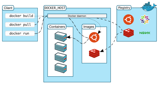
Docker architecture

Here is short definition of each docker architectural component:

  • Docker deamon: Also called dockerd, it is the main process used by Docker to manage containers through API requests made by the docker client.
  • Docker client: This is the interface that makes possible the interaction with Docker; all the command base requests are sent to the docker deamon to start, stop, or simply manage a container.
  • Docker registries: A local (private) or public (Docker Hub) repository where Docker images are stored, images are pulled from docker registry through the docker client using the docker pull command.
  • Docker objects:
    • Images: A snapshot of a set of files required to run an application, images are created using a Dockerfile which contains a set of instructions that makes possible the creation of this binary file.
    • Container: It is the runnable instance of a docker image, nothing more than a program executed in the docker deamon machine.

The following diagram was taken from the Docker documentation website; it is the graphical interpretation of Docker’s architecture:

Taking the concepts defined previously and also analyzing the architecture diagram above, you can say Docker is a platform designed to work under the client-server model architecture where the main docker process (dockerd) runs in the form of a daemon in a local or remote server/computer that is accessible through the network by a command line client called Docker client. The client allows you to execute Docker commands against the Docker deamon to build, run and distribute Docker containers.

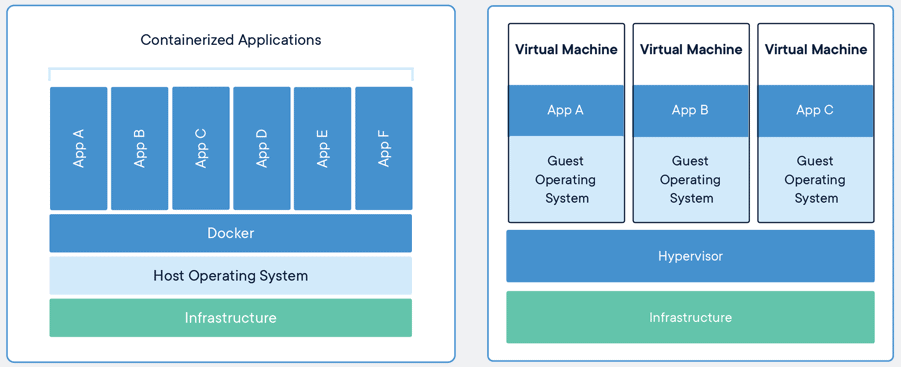
Docker vs VMs

No question about it, making a comparison between Docker containers with VMs is sometimes inevitable. Virtualization technology has been widely adopted and implemented in the IT industry for at least the last 15 years, but Docker is a game changer.

Virtualization is basically a way to run multiple operating systems and applications on a single server to take full advantage of its processing power. Each virtual machine has all the hardware resources virtualized by a hypervisor which is the server that makes it possible to run multiple operation systems. Each VM will always include a full copy of an operating system, the application, necessary binaries, and libraries.

Containers run directly in the host machine like any other normal application or process, thus no hardware virtualization is required. Unlike VMs, containers share the host operating system kernel, which means the virtualization occurs at the operating system level delivering a better performance and efficient resource management (less storage).

Another advantage of containers over VMs, is that all the code, libraries, and dependencies of an application are already installed and included in the container image. That means you don’t have to worry about finding all those dependencies or even to standardize software deployments like a SQL Server installation.

Based on the Docker characteristics above, it makes sense to make Docker as essential part of

continuous integration and continuous delivery (CI/CD) workflows given the low risk, portability, automation, and scalability.

Installing and Running Docker on macOS

Installing Docker on macOS is no different than any other conventional application for this platform; the installation process is very straightforward, and the instructions are easy to follow.

Before starting with the installation process, I would like to take a moment to review the list of system requirements that your laptop must meet in order to run Docker in macOS:

  • A minimum of 4 GBs of RAM
  • macOS El Capitan (10.11) or newer versions
  • Hardware must be at least from 2010 or newer
  • At least 10 GB’s of free space on disk

Apart from the system requirements, Docker as a platform requires the creation of a Docker ID account at Docker Hub. Without this ID account, you will not have access to the Docker Hub repositories like Microsoft’s official repository, RedHat, Ubuntu, etc.

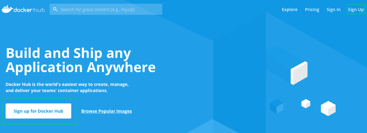
The Docker ID account becomes your personal repository which you can use later to upload custom images. Go to the sign up page:

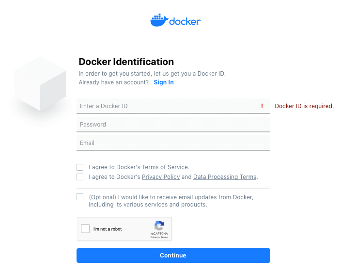
Click on Sign up for Docker Hub, enter a username to use as your Docker ID, then a valid email address. Finally, enter your password. Of course, do not forget to check the terms of service, privacy policy, and Data Processing terms.

The password must be at least 6 characters long. Then you have to wait for a confirmation email:

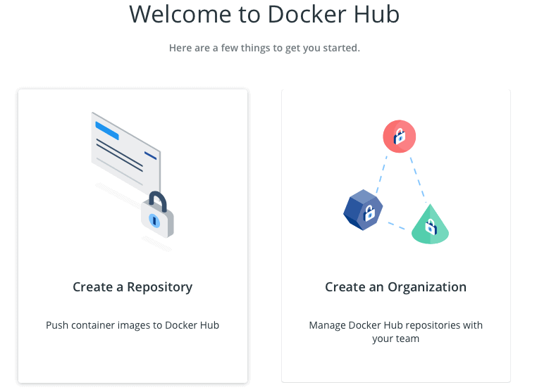
Once your email is verified you are in, welcome to Docker Hub! Now it is time to create your personal repository, you will use this workspace later to upload and share custom Docker images.

Click on the Create repository option on the left of the screen:

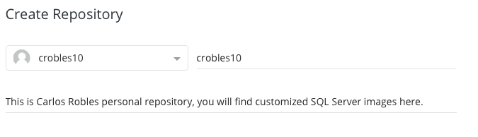
Now you have to choose the Docker account to own the repository, in this case use the account you just created. Then provide a name, as you can see from the image below, I’m using the same name as my Docker Hub account, but it is really up to you. The requirements for the repository name, is to contain a combination of alphanumeric characters and may contain special characters.

You can even add a repository description if you want; this is like a short description or tagline for your Docker Hub account to describe the meaning of your personal repository. For example, I’m describing my repository as a place where you can find customized SQL Server Docker images.

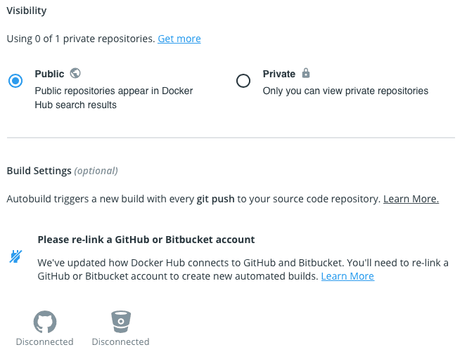
Now move on with the next option, specifically visibility. It can be Public or Private. I will recommend using Public, so that you can collaborate with friends or colleagues. You can choose private in case you are looking for an enterprise type of collaboration within your organization.

It is important to mention that Docker provides only one free private repository per Docker Hub account. If you need more, you have to upgrade your Docker Hub account to a billed plan.

The Build Settings is optional. You can link your GitHub account with your Docker Hub repository to automatically push images to your source code repository. I will skip this option for now, because this is not in the scope of this article.

Once you are done with all the configuration, then simply click Create at the very bottom of the page.

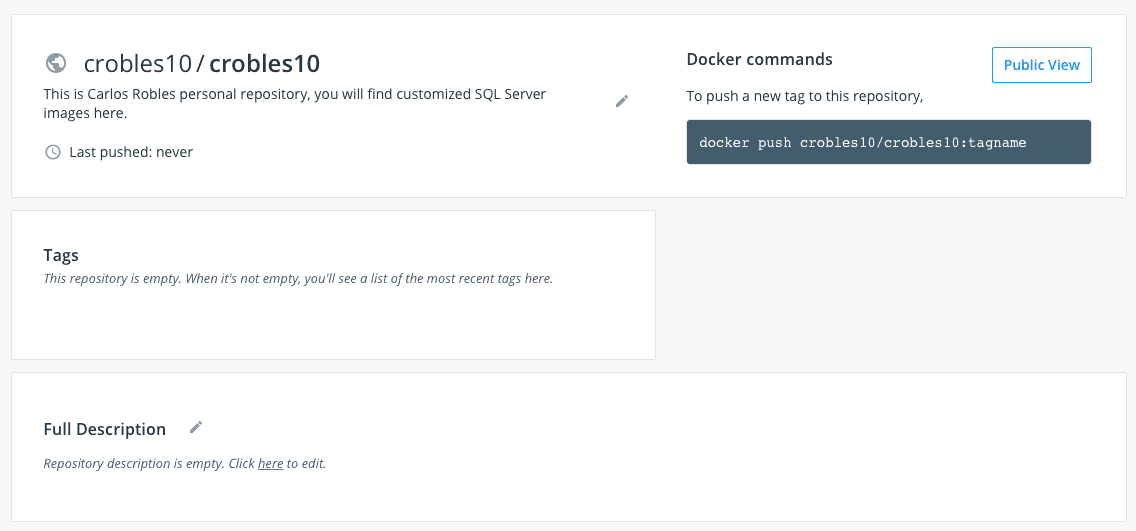
If you have completed all the steps successfully, you will be redirected to page where you will be able to see how your personal repository looks. You can add tags or a full description if you want. It is important to note the docker commands section on the right upper side:

The Docker push command described there, shows how you can upload custom images to this repository. It will vary depending the name of the Docker Hub and the repository name; in my case I use the same for both.

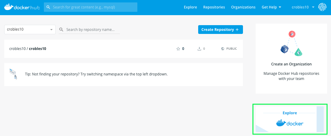
Now you are all set. It is time to download Docker’s software for macOS. Go to the main site and click on Docker hub at the very top of the screen. Then go to explore:

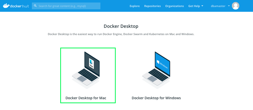
You will see the two Docker desktop option, obviously, you are interested in the Docker Desktop for Mac:

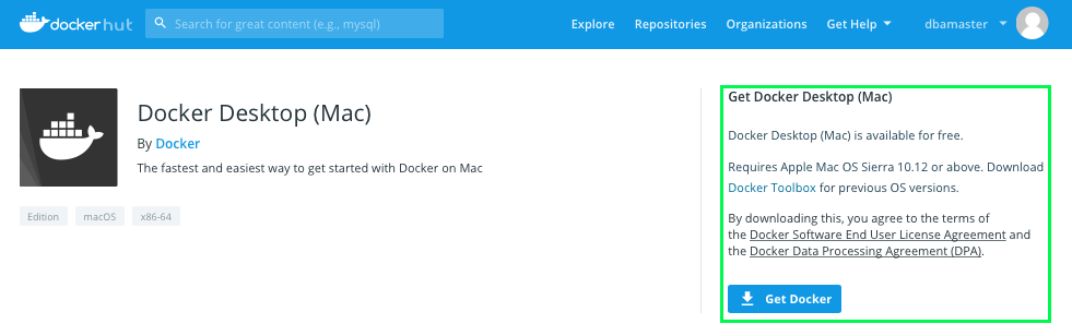
Look on the right top corner and click on Get Docker:

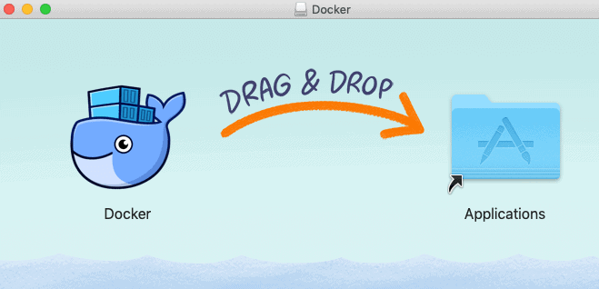
Once the Docker installer (dmg file) shows up in your download folder, double click the file called Docker.dmg to start the installation. A pop-up window will be displayed on your screen:

As the instructions suggest, just drag the blue whale icon (Moby) to your applications folder. Once the copy process completes, a new Moby icon will show up in your macOS bottom dock or in the application folder: (depending on how you have your settings configured)

At this point, you have Docker successfully installed and ready to roll. Begin by clicking on the blue whale icon and waiting for the docker daemon to automatically start.

Once started, Docker will automatically create a new icon at the macOS menu bar; this icon shows the Docker deamon’s current status.

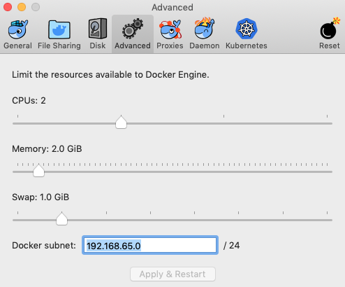
As an additional step, I recommend taking a look at Docker’s preferences to personalize the resource utilization, like CPU and memory.

Docker by default uses 2 GBs of RAM for the Docker engine. I personally like to give it a little boost changing it to 4 GBs. The CPU is a little bit different. Docker will allocate half of the number of processors available on your machine. Of course, this number can be decreased or increased according your needs and preferences.

Microsoft Container Registry (MCR)

Docker containers are starting to gain acceptance across multiple software vendors. Docker hub is the public repository where anyone can have access to the latest certified images published by vendors using Docker container images.

By mid-2018, Microsoft created its own syndicated central repository called the Microsoft Container Registry (MCR). The goal of this new centralized repository is to have one source for all the container images available in the Docker Hub and Red Hat Container catalog.

This means, all new container images will be published in the Microsoft Container Registry, and all existing containers images will exist on Docker Hub.

Microsoft’s Docker hub repository provides information about the catalog of official images for SQL Server on Linux running on the Docker engine. If you look carefully at the bottom of the Linux images table, there is section that provides the URL.

This URL it will redirect you to a JSON format website that contains the complete list of images. This is great, but there is another way to retrieve the same list using the Docker’s HTTP API V2.

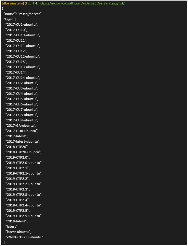
Docker’s HTTP API V2, has a GET method which will return the complete list of images for a known repository. All you have to do is to use the curl command. Open the macOS built-in terminal (Applications>Utilities) and execute the following command:

curl -L https://mcr.microsoft.com/v2/mssql/server/tags/list/

You’ll see a list of images in the repository.

As you may have noticed already, each image has a unique name called a tag. This tag is used to self-describe each image. It consists in a three-part name composed as follows:

Image tag description:

SQL Server Version – build number – operating system

The first part describes the SQL Server version, the second is the build number, and the third is the operating system.

For example, if you want to create a container based on SQL Server 2017 CU14 for Ubuntu the tag you want to use is “2017-CU14-ubuntu”.

Combining this tag with the docker pull command you get:

docker pull mcr.microsoft.com/mssql/server:2017-CU14-ubuntu

This Docker command will download an image of SQL Server 2017 CU14 for Ubuntu into your local image repository for later use when executing the docker run command.

Docker Client Commands

In order to familiarize yourself a little bit more with the Docker client, you will need to invest a little time exploring all the docker commands.

As you may have noticed, in order to interact with the docker client you need to use a command line interface. In the case of macOS, you have the built-in terminal (Applications>Utilities). You may want to add this application to your dock for quick access. From now on, all the input and output you will see for all the Docker commands will come from the Terminal application.

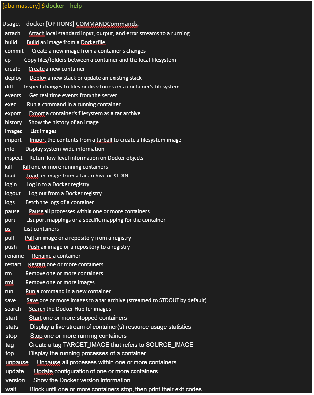
These commands are not that hard to learn, the docker –help command provides the list of all the available commands in the docker engine:

In case you would like to learn about each one of the commands in detail from the list above, I strongly recommend that you check the Docker online documentation which includes detailed information of each command including examples.

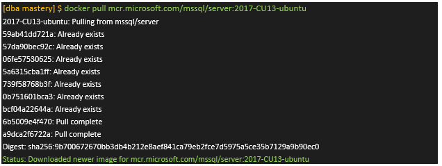
Here is a quick example of how to use the docker pull and docker run commands to create a SQL Server container. The first thing you must do is to download (pull) a valid image from the Microsoft Container Registry. This example uses the SQL Server 2017 CU13 version for Ubuntu.

docker pull mcr.microsoft.com/mssql/server:2017-CU13-ubuntu

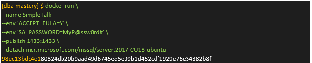
The output of the docker pull command confirms the image with the tag “2017-CU13-ubuntu“ is available in the local repository. Now create (run) a SQL Server Docker container called SimpleTalk:

docker run \
--name SimpleTalk
--env 'ACCEPT_EULA=Y' \
--env 'SA_PASSWORD=MyP@ssw0rd#' \
--publish 1433:1433 \
--detach mcr.microsoft.com/mssql/server:2017-CU13-ubuntu

An output for the docker run command includes just an ID (highlighted in yellow). What does this mean? How do I know if my SQL Server container is up and running?

You can answer these questions using the docker ps command, which is going to list all the active containers running in my Docker host machine.

docker ps --format "table \t\t"

Here is the example of the output of this command:

Noticed, I have applied a filter to show me just the ID, the name and the status of the container. If you look carefully the Container ID (98ec13bdc4e1) from this output matches the one highlighted in yellow that was returned when the container was created.

It is remarkable how easy and simple is to use Docker to create SQL Server instances in matter of seconds, yes you read it right just seconds! You can confirm that by reviewing the status column from the docker ps command. It shows that my container called SimpleTalk has been up and running for the last two seconds.

Conclusion

Easily and quickly creating a “sandboxed” SQL Server instance is a game changer for the many developers using macOS. In this article, you installed Docker and created your first container.

Please join me in this series of articles where I will be talking the following topics related to Docker containers for SQL Server:

  • Docker container management
  • Persistent storage \ Docker volumes
  • Transferring files from the host machine to Docker and vice versa
  • Restoring databases from any source to a SQL Server instance running in a container
  • Upgrading a SQL Server instance running in a container
  • Connecting to a SQL Server in a container using SSMS
  • Connecting to a SQL Server in container using Azure Data studio
  • Creating a custom SQL Server container
  • Automating the deployment of custom SQL Server containers
  • Configuring an Availability group for a SQL Server instance running in a container
  • More …

Thanks for reading!

The post Creating Your First SQL Server Docker Container in macOS appeared first on Simple Talk.


from Simple Talk http://bit.ly/2Yx6tW3
via

Thursday, May 9, 2019

The Phantom Menace in Unit Testing

Let me state up front that this is not a rant about unit testing; unit tests are critically important elements of a robust and healthy software implementation. Instead, it is a cautionary tale about a small class of unit tests that may deceive you by seeming to provide test coverage but failing to do so. I call this class of unit tests phantom tests because they return what are, in fact, correct results but not necessarily because the system-under-test (SUT) is doing the right thing or, indeed, doing anything.

In these cases, the SUT “naturally” returns the expected value, so doing (a) the correct thing, (b) something unrelated, or even (c) nothing, would still yield a passing test. If the SUT is doing (b) or (c), then it follows that the test is adding no value. Moreover, I submit that the presence of such tests is often deleterious, making you worse off than not having them because you think you have coverage when you do not. When you then go to make a change to the SUT supposedly covered by that test, and the test still passes, you might blissfully conclude that your change did not introduce any bugs to the code, so you go on your merry way to your next task. In actuality, you simply do not know if you introduced any bugs because your test (or tests) are not reporting valid information.

Invoking Some Spirits

What exactly is a phantom test? Consider this example. Say you have a function AccumulateWhenGreen(value, condition). The parameters are:

  • Value — the number to add to the accumulation
  • Condition — red, yellow, or green indicating some status

The name infers that it should accumulate the given value when the condition is green and skip the value when the condition is red or yellow. To evaluate the function, write a unit test (this is in pseudo-code rather than any particular language).

Test “AccumulateWhenGreen skips value when red”
{
Accumulator <- 0
 AccumulateWhenGreen(23, Condition.Red)
Assert Accumulator = 0
}

If that test passes, the function has successfully fulfilled that clause in the contract, right? (By contract I mean the software requirements to be implemented.) Not so fast. Look at the pseudo-code for AccumulateWhenGreen itself:

Function AccumulateWhenGreen(Value::int, Condition:: ConditionType)
{
If (Condition is ConditionType.Green)
Then Accumulator <- Accumulator + Value
Else DoNothing
}

That code is correctly written to implement the relevant requirement. However, do not take my word for it– prove it. Change the test, so the second argument passed to AccumulateWhenGreen is Condition.Green instead of Condition.Red. What happens to the test? Now the test fails, because the value gets added to the accumulator and thus the accumulator is non-zero. Finally, change the parameter to Condition.Yellow and the test again passes. Q.E.D.

So far so good. Now consider this alternate implementation of AccumulateWhenGreen:

Function AccumulateWhenGreen(Value::int, Condition:: ConditionType)
{
Accumulator <- Accumulator + Value - (((Value * 3) + 6) / 3) + 2
}

At first glance, it looks like this does some convoluted computation to make that code do what it is supposed to. Moreover, the “AccumulateWhenGreen skips value when red” unit test will pass: the accumulator will not be changed. Is it because that computation somehow takes the input value “23” into account? No; the unit test will pass for any integer you care to provide to the function. That’s good, right? Why is the code working? The answer is that it is not. Sure, the test passes for Condition.Red. It also passes for Condition.Yellow. Fine. However, for Condition.Green, the test still passes when it should fail, because the accumulator is supposed to change for Condition.Green.

At the very beginning I mentioned three things the code could do:

(a) the correct thing

(b) something unrelated

(c) nothing

In this case, the code is doing something unrelated. Notice that the Condition argument is suspiciously absent from the calculation. Paraphrasing a professor from my university days, the code is providing an answer to some question, just not the correct one! Consider the third alternative, doing nothing. With this code…

Function AccumulateWhenGreen(Value::int, Condition:: ConditionType)
{
DoNothing
}

…and get the same results: the unit test passes for Condition.Red and for Condition.Yellow – both of which are good news – and for Condition.Green, which is bad news.

How to solve this? Recall above that, with the correct code in place, the test passed for Condition.Red or for Condition.Yellow but failed with Condition.Green. One way to avoid the phantom menace is to add more tests:

Test “AccumulateWhenGreen skips value when red”
{
Accumulator <- 0
 AccumulateWhenGreen(23, Condition.Red)
Assert Accumulator = 0
}

Test “AccumulateWhenGreen skips value when yellow”
{
Accumulator <- 0
 AccumulateWhenGreen(23, Condition.Yellow)
Assert Accumulator = 0
}

Test “AccumulateWhenGreen adds value when green”
{
Accumulator <- 0
 AccumulateWhenGreen(23, Condition.Green)
Assert Accumulator = 23
}

With this suite of tests in place, the correct code–case (a)–passes all three tests, but the incorrect code–cases (b) or (c)–fails on the third test.

Maxim #1:

A test checking that nothing happened

must be accompanied

by a test checking that something happened

Notice that the tests for Condition.Red and for Condition.Yellow passed with the correct code, unrelated code, or no code under test. That is, they always passed. Do they actually serve a purpose then? Yes! At this moment, those tests always pass, so you may conclude that if they pass, they provide no useful information about the correctness of the SUT. However, if down the road, upon making changes to the SUT they start failing, then those changes did introduce some problem.

Maxim #2:

A phantom test proves nothing if it passes.

It indicates a real problem if it fails.

Can you make a phantom test more solid (pun intended)? That is, can you make a test that is supposed to confirm nothing happened mean that nothing happened correctly? (Again, that means (a) the SUT has correct code rather than (b) unrelated code or (c) no code.)

Yes! Bring on our guest practice for this segment — test-driven development (TDD). Whether or not you use TDD, whether or not you write your tests first or last, the following can help you do (apologies to non-native English speakers for being cute here!) well, nothing. More formally, the following can help you create purportedly phantom tests—tests that confirm that nothing happened—in a way that you can have confidence that the code did that no-op in a correct manner.

TDD principles state that when you want to add new functionality, you first add a new test and that the new test must fail. If it does not fail, then either you have added a test for something your system already does, and presumably you already have a test for already, or you have added a phantom test, and the test will always pass.

Here is one way the story might have unfolded with our sample code and tests:

Create the first, happy path test:

Test “AccumulateWhenGreen adds value when green”
{
Accumulator <- 0
 AccumulateWhenGreen(23, Condition.Green)
Assert Accumulator = 23
}

Write some code to make it pass:

Function AccumulateWhenGreen(Value::int, Condition:: ConditionType)
{
Accumulator <- Accumulator + Value
}

Add the next two tests together:

Test “AccumulateWhenGreen skips value when red”
{
Accumulator <- 0
 AccumulateWhenGreen(23, Condition.Red)
Assert Accumulator = 0
}

Test “AccumulateWhenGreen skips value when yellow”
{
Accumulator <- 0
 AccumulateWhenGreen(23, Condition.Yellow)
Assert Accumulator = 0
}

Both of those tests will fail. By Maxim #2, that says there is a problem to fix, as there should be. Write some more code that makes those tests now pass, adding the conditional in this case:

Function AccumulateWhenGreen(Value::int, Condition:: ConditionType)
{
If (Condition is ConditionType.Green)
Then Accumulator <- Accumulator + Value
Else DoNothing
}

With that in place, all tests pass. Moreover, those two new tests are now purportedly phantom tests. However, they began as failing tests and turned into passing tests as the code evolved, so they have provided value.

Maxim #3:

How you arrive at a phantom test matters.

I illustrated the above with TDD because it is vital that when you introduce a new test that it first fails. You can sometimes meet this requirement in a non-TDD fashion, but it takes more work. Either you need to add some more logic to your test to get to a state where it will fail, or you need to break your working SUT so that the test fails. Once you confirm that the test is failing for the right reason, then make it pass by backing out those artificial tweaks.

A Real-World Example: The Authorisation Problem

Sometimes you have to live with the presence of phantom tests, but often you can convert them to real, non-phantom tests. To illustrate this point, turn from the above academic example to consider a real-world example. Say you are designing an authorisation system to regulate access rights to resources in your enterprise system. One typical foundation of such an authorisation system might succinctly be:

User U is authorised to perform an action A if there is a policy that allows U to perform A and there is no policy that denies U from performing A.

Here are the tests you might come up with.

T0 – With no policies, an action is denied

That certainly is part of the contract because, per the stated requirement, there is no policy allowing the action, therefore the result should be denied.

T1 – With a policy allowing an action, the action is allowed

Clearly, from the requirement, the presence of such a policy should result in the action being allowed. Designate this policy P1, as you will use it again shortly.

Next, the test to confirm that when there is a policy that denies U from performing A, the authorisation decision is, in fact, “denied”.

T2 – With a policy denying an action, the action is denied

Here create a single policy P2 that denies U from performing A and check the resultThe result should be “denied,” but what does that tell us? If you remove P2—where you now have no policies at all—then check the result; it will still come back with “denied”. Why? Because there was no policy allowing A. This test is a classic phantom test: the requirement is to test that the presence of P2caused the outcome to be denied. Yet removing P2 yielded the same result, so the fact that the test passes does not prove anything.

You could turn this phantom test into a solid test, though, by bringing in policy P1 that was created earlier. It allows U to perform A. Thus, instead of using just P2 in this test use P1 + P2. If the result is “denied,” it is due to the presence of P2. Can you prove that? Certainly. If you remove P2 the result will be “allowed” because there exists a policy (P1) that allows U to perform A. Therefore, the test will fail. This test—with P1 + P2—is now a solid test!

Maxim #4:

Whenever possible convert phantom tests to real tests.

Conclusion

Phantom tests are sneaky. They can be hard to spot, and they provide a false sense of security. You have taken the first step to combat phantom tests just by being aware of their existence. When you do uncover a phantom test, look for ways to turn it into a solid test, so that it does not always pass. You should be able to make the test fail then, by adding in the key thing you want, make it pass. If, however, you must have a test that checks for nothing happening, make sure it is at least accompanied by a test that checks for something happening, too.


The post The Phantom Menace in Unit Testing appeared first on Simple Talk.


from Simple Talk http://bit.ly/2Vpt75B
via

Why DBAs Must Embrace DevOps

A good day for a database administrator (DBA) is a lot like a good airline flight. A lot of excitement in either situation is bad. In a perfect world, a DBA will be productive and not spending most of their time “putting out fires.” (And fires are never a good idea on a flight!)

DBAs are expected to keep their systems up and running smoothly and securely. Developers, on the other hand, must deliver new features at an ever-increasing pace. Often these features require changes to infrastructure, including database changes, which may seem like introducing chaos into otherwise stable systems.

It’s obvious that developers and DBAs have conflicting goals, but both stability of systems and quickly delivering features which bring value to the customer are critical to an organisation’s success. Traditionally, developers could just write code to fulfil a set of requirements, and then let someone else, the operations side, figure out how the code should be implemented. These changes, including changes to the database, can be bottlenecks as the DBA and other operations folks ensure that the changes are safe and there is minimal disruption. There is often poor communication between teams and lots of blame to spread around when things go wrong.

One may conclude that the developers should just slow down and stop creating all this change, but companies that don’t innovate – and quickly – will be replaced by those that do. On the other hand, customers will also move on to other suppliers when services are not available due to unplanned outages.

To solve these problems, organisations are embracing DevOps methodologies to quickly bring value to customers while maintaining stability and decreasing deployment failures. DevOps is not a prescriptive set of steps to follow, nor a framework like Agile. It’s more of a culture change that begins by building communication and trust among teams and breaking down the silos between them. It also means smaller, more frequent releases of code. Instead of a couple of large deployments with lots of changes every month, some companies have many deployments each day with a small number of changes in each.

The latest State of Database DevOps survey found that 58% of the organisations participating had already adopted DevOps across some or all projects, and 27% planned to do so in the next two years. It also found that 66% did not include the database as part of the automated build and deployment process! There are often database changes, like new tables or columns, that must be deployed along with application changes, so this can be the bottleneck that slows down the delivery of new features.

With the right tools, DBAs can include databases in source control and generate deployment scripts that can be integrated smoothly with the changes from the other teams. Dev, test, QA, and staging databases that resemble production can be created in seconds, and private information can be sanitized automatically. Automating these tedious, time consuming steps that are so important for the DevOps pipeline frees up the DBA’s time so that they can focus on the things that require their expertise like stability, performance, availability, and security.

It isn’t easy to automate database changes so that they stay in sync with application changes, but there are companies doing it and doing it well. The only way to accomplish this is for DBAs to embrace DevOps.


Commentary Competition

Enjoyed the topic? Have a relevant anecdote? Disagree with the author? Leave your two cents on this post in the comments below, and our favourite response will win a $50 Amazon gift card. The competition closes two weeks from the date of publication, and the winner will be announced in the next Simple Talk newsletter.

The post Why DBAs Must Embrace DevOps appeared first on Simple Talk.


from Simple Talk http://bit.ly/2Yi5iJO
via

Wednesday, May 8, 2019

The BI Journey: The Journey Begins

The series so far:

  1. The BI Journey: The Analyst
  2. The BI Journey: The Expert’s Advice – Part 1
  3. The BI Journey: The Expert’s Advice – Part 2

Stephen, the sales manager, was impressed with the work of his intern, Ruthie, the Business Analyst. She had taken a seemingly off-hand conversation about how Stephen’s friend was looking at using analytics to help drive business, and within a couple of weeks churned out her solution for Stephen’s department. Stephen, who heads Sales for AdventureWorks had always had a problem trying to figure out how well various parts of the department were functioning. With the business intelligence solution that Ruthie came up with, Stephen now had some idea about how the department was faring. There was a lot more he wanted to know and had ideas that he could implement if he had the right information. However, from what Ruthie had given him, despite it being a small report, Stephen could see a lot of value – and that was the key. He wanted to capitalize on it.

From Value to Ideas

He felt that Ruthie had put in a lot of genuine effort into the solution that she had built. She had taken initiatives, even as far as consulting with folk from the technical community, while doing much research of her own. More than anything, he found that she had a passion for what she had been doing all along. Since the sales department had never had a business analyst before, Stephen decided he would hire Ruthie as the department’s permanent business analyst.

For now, Stephen wanted to give Ruthie more responsibility. After seeing the capabilities that Power BI provided, and how they could utilize its various features, he wanted a complete solution so that the entire sales department would be data-driven. This included Stephen being able to build reports on his own and the sales team running the quarterly sales meeting from a single dashboard. Ruthie would manage the solution including development, standards and governance, and routinely enhancing and improving the solution. She would also train the sales personnel on how to use the solution and create reports.

Ruthie was overwhelmed and overjoyed at the same time when Stephen told what he had in store for her. She accepted the responsibilities without giving it a second of thought.

Going Big

One of the things she learned about during conversations with George, her mentor, was data warehouses. Data warehouses are large databases that consolidate information from different systems and make the data available for business intelligence purposes. Much like a Power BI data model thought Ruthie. A data warehouse is considered the single source of truth across the organization for business intelligence. She had attended a meetup of the local data community and had been quite taken by the presenter that week. Lisa, a data architect at a consulting firm, had talked about data warehousing and business intelligence in great depth.

Ruthie was even more convinced about the need for a data warehouse when she received a text message from Stephen while she was at the meetup: “Ruthie, I’ll need you to give marketing access to our BI solution. I’m getting some funding from them 😊

She had spoken to Lisa after the meetup and inquired about getting started with a data warehouse at her workplace. She told her about her new responsibilities, and that the talk had inspired her to build a data warehouse for the sales department.

Lisa had loved Ruthie’s enthusiasm and had been impressed when she heard about the responsibilities given to her and even more at the level of attention Ruthie had paid to what she had presented. But she had told Ruthie to hold on and had proceeded to explain why she should not be looking at a data warehouse at this stage.

Data Warehouse – Not Now

Lisa had explained to Ruthie that a data warehouse needed a lot of effort to build, which required a considerable amount of time spent on gathering requirements for the right set of dimensions and facts, for the measures and KPIs that the users needed, the calculations for these measures and KPIs, and the reports that users wanted.

A data warehouse also needs a data integration component that routinely brings in data and transforms it to fit the data warehouse. Building a data integration component to satisfy all the requirements takes quite a lot of effort. Data integration is considered to be the most significant component of a data warehousing solution in terms of effort and complexity to build. It’s so much effort that teams often segregate it as a separate project in the data warehousing solution.

Talking from experience, Lisa had explained that more often than not, requirements keep changing, especially when users are looking at reports and suddenly want something that is not there. If the requirements for the dimensions and facts were not correctly defined, or if the users came up with a change to the logic, you would find yourself repeatedly modifying the data warehouse, and then modifying the data integration process to match the changes you did on the data warehouse. All this would then elongate the time taken to build your data warehouse.

Therefore, Lisa had told Ruthie, if you were even looking at building a data warehouse incrementally, you would need to be sure of all the requirements of at least one logical chunk of the data warehouse. This way you could develop it, test it, ship it, and then move on to the next chunk. However, it’s not feasible to develop this one chunk iteratively as a data warehouse. Micro-iterations are a no-no. In Ruthie’s case, said Lisa, since it was just Ruthie, and a bunch of salespeople, a data warehouse was out of the question. Micro-iterations were part of the deal here.

Finally, Ruthie would have to learn at least a couple of new technologies. The most straightforward implementation of a data warehouse would require Ruthie to learn a database management system such as SQL Server, querying basics, a querying language such as T-SQL, an integration technology such as Integration Services, and configuring all of these technologies, explained Lisa. Alternatively, if she were looking at the cloud, Ruthie would need to understand how things worked on the cloud, pricing for the technology services that she was planning on using, a database management system such as Azure SQL Database, integration technologies such as Azure Data Factory and Integration Services, along with a querying language like T-SQL. Either that or Ruthie needed to have at least a couple of developers who had the experience to do the work. This was not a luxury that Ruthie or Stephen had.

Lisa advised Ruthie that a data warehouse was a long way from what was needed for the Sales Department. What she needed was a solution that provided value fast. To do that, she needed a familiar tool that allowed quick development and allowed her to make updates fast. She also reminded Ruthie about technology costs which were something Ruthie had not considered.

Lisa’s advice to Ruthie was:

  • Leverage Power BI and sketch out an outline of a solution
  • Figure out the costs for the solution, and get approval
  • Set up a list of tasks in a backlog
  • Get started!

Preparation

Ruthie was pleased about her conversation with Lisa. Lisa had volunteered to help, and Ruthie was ecstatic that she had another mentor. Being part of a technical community had many benefits. She hoped one day to give back.

She met George (who was good friends with her by now) after the meetup for coffee and to run through the notes she had jotted down.

The first thing that Ruthie had done was to put down a backlog of high-level steps:

  1. Solution outline
  2. Calculate cost
  3. Plan the development
  4. Develop solution

Solution Outline

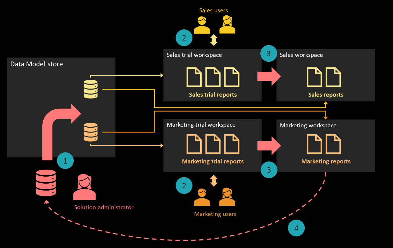
Looking at the requirements that came from Stephen, Ruthie had already understood that creating a separate data model each for each report was not going to work. That’s why she had been thinking of a data warehouse in the first place. However, after the “consultation” she had with Lisa, she now looked at replicating the same concept using the tools she was quite familiar with, in this case, Power BI. Ruthie’s idea was to build a data model that encompassed all the data required by the sales department. Currently, she had one data model built off three dimensions and a couple of fact tables. The facts on these tables had measures built on top of them, and Ruthie planned on extending this data model further. She had a plan for the flow of the solution, so she put that down.

Figure 1: Solution outline

The flow of the solution was quite simple:

  1. The solution administrator will develop data models and deploy to the data model store.
  2. Sales and marketing users will build reports using their respective data models and publish these reports in the trial workspace.
  3. After reviewing the published reports, either on a scheduled or as requested, selected reports will be published to the main workspace of the respective departments.
  4. Any newly identified measures, metrics, and even dimensions modifications will be pushed to the next iteration of the data model.

The solution administrator runs the show, and Ruthie decided to assume that role.

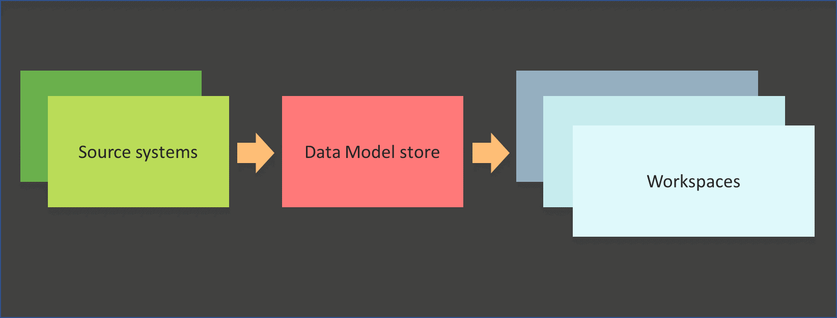
She then put down the components of the solution in a diagram. George liked it the moment she showed it to him. He called it an architectural diagram. Ruthie beamed. Grasshopper had learned fast.

Figure 2: Architecture

Cost

When she thought about the cost, Ruthie cringed. She had always been uncomfortable when it came to handling others’ money, including telling others how and how much they should be spending. Figuring out the cost of technology was something new to Ruthie. However, since she was looking at a simple solution and one that was made up of a tool she knew quite well, she decided that she could figure it out.

She used the architectural diagram to list the technologies that were needed, counted the number of users that required the software, and performed some basic math. Ruthie chose Power BI since she had already started using it and was quite the expert with it now. She ran it by George, and he said that it looked good.

Figure 3: Technology cost

Plan

With the new responsibilities that Stephen had given Ruthie, he expected visibility on the progress. Hence why he wanted her to give him a plan. Ruthie was not sure how to plan for the work since all the work Ruthie had done previously had been ad hoc.

She decided that the most sensible thing she could do was to take a logical approach and list the high-level items she planned on doing. She then did a guestimate of the time it might take for each task. She then grouped up these tasks with a 15% buffer to fit into three weeks. She called each three weeks an iteration, and came up with a plan for the next two months:

Iteration 1:

  1. Orders (with Customer, Product, Salesperson, Date)
    • Configure the current solution to use the sales database instead of files
    • Port the solution to fit the new architecture
  2. Train pilot sales personnel to build reports from the published data model
    • Pilot sales personnel will start building reports after this
  3. Complete Customers, Product, Salesperson dimensions with all possible attributes and hierarchies
  4. Sales personnel to provide feedback

Iteration 2:

  1. Add three new complete dimensions
    • Dimensions to be identified based on sales personnel priority
  2. Build measures that make use of new dimensions (if any)
  3. Deploy changes to sales and marketing workspaces
  4. Review sales personnel’s reports and target reports for promotion to the main workspaces from trial workspaces
  5. Plan new measures, metrics and dimension modifications to include in the next iteration

Iteration 3:

  1. Add three further complete dimensions
    • Dimension to be based on sales personnel priority
  2. Build measures that make use of new dimensions (if any)
  3. Add new measures, metrics and dimension modifications identified from reports built in Iteration 2
  4. Deploy changes to sales and marketing workspaces
  5. Review sales personnel’s reports and target reports for promotion to main workspaces from trial workspaces
  6. Plan new measures, metrics and dimension modifications to include in the next iteration

The next day she presented the solution overview, cost matrix and plan to Stephen. Stephen liked what he saw and gave Ruthie the go-ahead to start implementing the solution the following week. By then he would have the budget organised for the project and the technology licenses in hand.

An Exciting Beginning

While a data warehouse is an excellent solution for an organisation’s business intelligence platform, it almost always requires a lot of effort to build and requires a significant cost. However, a data warehouse, a central repository of analytical data, should be an organisation’s goal if they are serious about analytics and business intelligence. A great way to get there would be to capitalise on the success of self-service business intelligence due to its agile and rapid development capabilities and channel the value it generates as input to build the data warehouse.

Ruthie had now proven herself capable and was given the responsibility of implementing the division’s business intelligence solution. Though small in scale, the scope for growth was quite big, Stephen, her boss, could see his business vision coming together, and he was glad that he had someone bright and passionate like Ruthie by his side. Something that had started as a lunch table conversation a few weeks ago had materialised into this: First a couple of reports, now the beginning of a solution. AdventureWorks’ BI journey had begun.

Note: To discuss the technical aspect of the ideas laid out in this article, await a companion article to be published soon.

The post The BI Journey: The Journey Begins appeared first on Simple Talk.


from Simple Talk http://bit.ly/2J90gM3
via

Thursday, May 2, 2019

Enjoying Joins in MongoDB

MongoDB has a prodigious appetite for unstructured data and has its place in a Database Developer’s toolkit. Even with indexes in place, some operations that involve aggregation are a lot slower than they are with relational databases: So it is when using ‘joins’ between collections. Lookup, the MongoDB equivalent to Joins, cannot yet do Merge joins or hash joins, so is never going to be fast in the current form. It is far more suitable for enumerations where there is a limited range of alternatives. We can help Lookup along by providing an index that allows it to do an index nested loops join, but beyond that we have difficulties in getting dramatic improvements in the performance of any ‘JOIN’.

We can, of course, argue that collections of documents render joins unnecessary, but this is only true of relatively static, unchanging information. Data that is liable to change is always best stored in one place only.

This article explains how to make such a MongoDB database perform reasonably when reporting historic and slowly-changing information.

Joins in MongoDB

Why bother with joins in a document database? As well as creating entirely new databases in MongoDB, we are beginning to see a lot more databases ported to MongoDB from the relational. These require a lot of lookups, especially for reporting. Some people argue that document databases should de-normalise the data to get rid of the requirement for lookups. I’m going to argue that, if you provide and maintain summary collections, known as aggregates or pre-aggregates, and you use a thread that is separate from the application in order to maintain them when the data in the tables change, then it doesn’t matter so much. It is the database equivalent to cooking the meal beforehand in the kitchen rather than requiring each guest to cook their own meal at the table.

Just as a test-bed, we’ll use a conversion to MongoDB of SQL Server’s classic practice database, AdventureWorks. I chose this because you need to do several lookups to get reports from it, and it can come up with some awkward migration problems that are useful for our purposes. It also allows us to do a direct comparison of the two database systems, though we do this with due warnings that it is like comparing apples and kittens. I include the extended JSON for this database with the article. It takes just a moment to load.

Querying without an index

For our example, we will start without any indexes and then add them later, making sure that they are being used by checking the timings. We will also use the MongoDB profiler to check on the strategy being used.

We execute the following SQL query in MongoDB using Studio 3T, a MongoDB GUI with a handy SQL Query feature:.

SELECT p.PersonType, Sum(soh.TotalDue), Count(*)
  FROM "Sales.SalesOrderHeader" soh
    INNER JOIN "Sales.Customer" c
      ON soh.CustomerID = c.CustomerID
    INNER JOIN "Person.Person" p
      ON c.PersonID = p.BusinessEntityID 
  GROUP BY p.PersonType
--Primary type of person: SC = Store Contact, 
--IN = Individual (retail) customer

It provides a result that tells us the number of individual customers and store contacts, and the total value of their orders. Our only change from SQL Server is to put string-delimiters around the name of the collection.

It has two joins, implemented by lookups. We bang the button. Five minutes and seventeen seconds later, it finishes. Soon afterwards, a concerned but reproachful person phones from the Society for the Prevention of Cruelty to Databases. She points out that a few indexes would have saved a great deal of anguish. (The cursor method cursor.maxTimeMS() only works with queries)

It is best to look at the auto-generated code at this point.

// Requires official MongoShell 3.6+
use AdventureWorks;
db.getCollection("Sales.SalesOrderHeader").aggregate(
    [
        { 
            "$project" : {
                "_id" : NumberInt(0), 
                "soh" : "$$ROOT"
            }
        }, 
        { 
            "$lookup" : {
                "localField" : "soh.CustomerID", 
                "from" : "Sales.Customer", 
                "foreignField" : "_id", 
                "as" : "c"
            }
        }, 
        { 
            "$unwind" : {
                "path" : "$c", 
                "preserveNullAndEmptyArrays" : false
            }
        }, 
        { 
            "$lookup" : {
                "localField" : "c.PersonID", 
                "from" : "Person.Person", 
                "foreignField" : "BusinessEntityID", 
                "as" : "p"
            }
        }, 
        { 
            "$unwind" : {
                "path" : "$p", 
                "preserveNullAndEmptyArrays" : false
            }
        }, 
        { 
            "$group" : {
                "_id" : {
                    "p᎐PersonType" : "$p.PersonType"
                }, 
                "SUM(soh᎐TotalDue)" : {
                    "$sum" : "$soh.TotalDue"
                }, 
                "COUNT(*)" : {
                    "$sum" : NumberInt(1)
                }
            }
        }, 
        { 
            "$project" : {
                "p.PersonType" : "$_id.p᎐PersonType", 
                "SUM(soh᎐TotalDue)" : "$SUM(soh᎐TotalDue)", 
                "COUNT(*)" : "$COUNT(*)", 
                "_id" : NumberInt(0)
            }
        }
    ], 
    { 
        "allowDiskUse" : true
    }
);

When you do a lookup in MongoDB, the key field that you specify in the aggregation stage is the field of the documents in the collection you are looking up. This field defines the documents that you will collect as an array of documents.

The $lookup process matches the foreign field with the local field from the input documents that come down the pipeline.

That key field might not exist in the referenced document, in which case it is assumed to be null. If you don’t have an index on the foreign field, it will do a full collection scan (COLLSCAN) query for each one of the documents in the pipeline. This gets expensive: we need index hits instead of table scans.

A note on indexes

If you need to fetch just a few fields from a collection, then it is far more efficient to include these fields with the actual query criteria in a ‘covering index’. This allows MongoDB to use the quicker strategy of returning a result from the index directly without having to access the document. It makes sense to do this with any query that is likely to be frequently executed.

Which fields should have an index?

  • Any ‘key’ fields that are used in lookups or searches to identify a particular document
  • Fields that are used as foreign keys
  • Where the key uses several fields, such as a Firstname/Lastname combination, it is best to use a compound index.
  • Where one or more fields is used for sorting.

It is a good idea to consider the way you want sorting to be done in reports, because this determines the best order for the fields in the index.

Creating the index

Whenever the relational tables have a single column as the primary keys, we’ve added them as the _id field as part of the import. These special _id fields work very much like clustered indexes. We have to call them _id to get them adopted as clustered indexes. We’ve added the original field under its original name so that queries don’t break. We just need create an index for all the other fields that are used for the lookup; the ‘from’ fields and also those which are referenced by the lookup; the ‘foreignField’. This is equivalent to what is specified in the ON clause of the JOIN. In this case, that means Sales.Customer.PersonID, Person.Person.BusinessEntityID and Sales.SalesOrderHeader.CustomerID. We change the primary key reference to Sales.Customer.CustomerID to use our already-indexed _id, which has the same values as customer_id.

We retest and the response comes down to 6.6 seconds This is better than the 5 minutes, 17 seconds without an index, but is a long way off what the original SQL Server database can do. On the same server as MongoDB, SQL Server manages the same aggregation in 160 ms.

Sadly, the MongoDB profiler cannot tell us much to help, beyond telling us that a COLLSCAN was used. This is unavoidable because, although individual lookups have quietly used an index, an index can’t easily be used as part of an overall aggregation unless it has an initial match stage.

If we change the order of joins in the SQL query in Studio 3T, SQL Server executes exactly the same plan as before, which is to do a hash match inner join on the customer and person tables, using clustered indexes scans on both tables, followed by an inner join of the result with SalesOrderHeader.

Here is the Studio 3T version:

SELECT p.PersonType, Sum(soh.TotalDue), Count(*)
 FROM "Sales.Customer" c
    INNER JOIN "Person.Person" p
      ON c.PersonID = p.BusinessEntityID 
    INNER JOIN  "Sales.SalesOrderHeader" soh
      ON soh.CustomerID = c.CustomerID
  GROUP BY p.PersonType
--Primary type of person: SC = Store Contact, 
--IN = Individual (retail) customer

In Studio 3T, the order of aggregation reflects the order of the joins, so the order of execution is different and better at 4.2 seconds. Optimising the aggregation script in the Aggregation Editor makes little difference to this, taking it down to just over three seconds. Basically, the optimisations consisted merely in reducing the fields being taken through the pipeline to just the essential ones

// Requires official MongoShell 3.6+
use AdventureWorks2016;
db.getCollection("Sales.Customer").aggregate(
    [
        { 
            "$project" : {
                "_id" : NumberInt(0), 
                "CustomerID" : 1.0, 
                "PersonID" : 1.0
            }
        }, 
        { 
            "$lookup" : {
                "localField" : "PersonID", 
                "from" : "Person.Person", 
                "foreignField" : "BusinessEntityID", 
                "as" : "p"
            }
        }, 
        { 
            "$unwind" : {
                "path" : "$p", 
                "preserveNullAndEmptyArrays" : false
            }
        }, 
        { 
            "$project" : {
                "CustomerID" : 1.0, 
                "PersonID" : 1.0, 
                "PersonType" : "$p.PersonType"
            }
        }, 
        { 
            "$lookup" : {
                "localField" : "CustomerID", 
                "from" : "Sales.SalesOrderHeader", 
                "foreignField" : "CustomerID", 
                "as" : "soh"
            }
        }, 
        { 
            "$unwind" : {
                "path" : "$soh", 
                "preserveNullAndEmptyArrays" : false
            }
        }, 
        { 
            "$project" : {
                "CustomerID" : 1.0, 
                "PersonID" : 1.0, 
                "PersonType" : 1.0, 
                "TotalDue" : "$soh.TotalDue"
            }
        }, 
        { 
            "$group" : {
                "_id" : {
                    "PersonType" : "$PersonType"
                }, 
                "SUM(TotalDue)" : {
                    "$sum" : "$TotalDue"
                }, 
                "COUNT(*)" : {
                    "$sum" : NumberInt(1)
                }
            }
        }, 
        { 
            "$project" : {
                "PersonType" : "$_id.PersonType", 
                "Total" : "$SUM(TotalDue)", 
                "Transactions" : "$COUNT(*)", 
                "_id" : NumberInt(0)
            }
        }
    ], 
    { 
        "allowDiskUse" : false
    }
);

If we continue to go down this route, it means we spend a lot of time optimising each query. We need to imagine that there are managers badgering us for a whole stack of revenue reports. What should we do instead?

Using pre-aggregation collections to simplify reporting

You are better off creating an aggregation collection that is at the lowest granularity you are likely to report on. This is the equivalent of an OLAP cube. In this case, we are dealing with records of trading taken from the invoices. These don’t change and there are good reasons why they shouldn’t. I’m always surprised to find historical data being fetched and aggregated every time there is a report. It would only make sense if there were time-travellers suddenly refusing to pay for their bicycles retrospectively (in the case of our example, AdventureWorks) or you were reporting on Enron’s data. In MongoDB we simply prepare and maintain our historical data in ‘pre-cooked’ form.

If we pre-aggregate with an intermediate collection such as this…

// Requires official MongoShell 3.6+
use AdventureWorks2016;
db.getCollection("Sales.Customer").aggregate(
    [
        { 
            "$project" : {
                "_id" : NumberInt(0), 
                "CustomerID" : 1.0, 
                "PersonID" : 1.0
            }
        }, 
        { 
            "$lookup" : {
                "localField" : "PersonID", 
                "from" : "Person.Person", 
                "foreignField" : "BusinessEntityID", 
                "as" : "p"
            }
        }, 
        { 
            "$unwind" : {
                "path" : "$p", 
                "preserveNullAndEmptyArrays" : false
            }
        }, 
        { 
            "$project" : {
                "CustomerID" : 1.0, 
                "PersonID" : 1.0, 
                "PersonType" : "$p.PersonType"
            }
        }, 
        { 
            "$lookup" : {
                "localField" : "CustomerID", 
                "from" : "Sales.SalesOrderHeader", 
                "foreignField" : "CustomerID", 
                "as" : "soh"
            }
        }, 
        { 
            "$unwind" : {
                "path" : "$soh", 
                "preserveNullAndEmptyArrays" : false
            }
        }, 
        { 
            "$project" : {
                "CustomerID" : 1.0, 
                "PersonID" : 1.0, 
                "PersonType" : 1.0, 
                "TotalDue" : "$soh.TotalDue"
            }
        }, 
        { 
            "$group" : {
                "_id" : {
                    "PersonType" : "$PersonType"
                }, 
                "SUM(TotalDue)" : {
                    "$sum" : "$TotalDue"
                }, 
                "COUNT(*)" : {
                    "$sum" : NumberInt(1)
                }
            }
        }, 
        { 
            "$project" : {
                "PersonType" : "$_id.PersonType", 
                "Total" : "$SUM(TotalDue)", 
                "Transactions" : "$COUNT(*)", 
                "_id" : NumberInt(0)
            }
        }
    ], 
    { 
        "allowDiskUse" : false
    }
);

… then our report drops from 4.2 seconds to 25 milliseconds.

In practice, I wouldn’t want to store such a specialised aggregation-collection. I would slice the more general report by a time period such as weeks, months, or years so that you can then plot sales over a time period. I’d also add the sales person’s ID and the ID of the store so that someone gets the credit for the sale.

Even with extra fields and more documents, you are still going to be in the same region of performance in creating the aggregation. If you use this technique, you have to maintain the cubes, or aggregation-collections, in just the same way as an OLAP cube whenever the data changes. This must be done as a scheduled job in background. If, instead, it was done as part of a user session whenever the aggregation was found to be out-of-date, then you could cause congestion, especially if a connection is shared.

Because I tend to think in SQL, I’ll rough out the aggregation I want. As the SQL is necessarily limited in what it can do, I leave out such things as the date calculations and the output stage.

SELECT c.PersonID, p.PersonType, soh.SalesPersonID, psp.Name, psp.CountryRegionCode,
  Sum(soh.TotalDue), Count(*)
  --,
  --Year(soh.OrderDate) AS year, Month(soh.OrderDate) AS month,
  --DatePart(WEEK, soh.OrderDate) AS week
  FROM "Sales.SalesOrderHeader" AS soh
    INNER JOIN "Sales.Customer" AS c
      ON c.CustomerID = soh.CustomerID
    INNER JOIN "Person.Person" AS p
      ON p.BusinessEntityID = c.PersonID
    INNER JOIN "Person.Address" AS pa
      ON pa.AddressID = soh.BillToAddressID
    INNER JOIN "Person.StateProvince" AS psp
      ON psp.StateProvinceID = pa.StateProvinceID
  GROUP BY c.PersonID, p.PersonType, soh.SalesPersonID, psp.Name,
  psp.CountryRegionCode
  --, Year(soh.OrderDate), Month(soh.OrderDate),
  --DatePart(WEEK, soh.OrderDate);

Getting the order right and tying up loose ends

Once this is running, I copy the mongo shell query code and paste it into the Aggregation Editor, Studio 3T’s MongoDB aggregation query builder.

I then fine-tune the aggregation:

Once this is executed, I can then do reports directly from Studio 3T’s SQL Query tab:

--total invoice value per year for AdventureWorks
Select Year, sum(Total)
  from "Sales.Aggregation"
  group by Year
  order by Year asc
  
--total invoice value per year for each country
--for AdventureWorks
Select Year, CountryRegionCode, sum(Total)
  from "Sales.Aggregation"
  group by Year,CountryRegionCode
  order by  CountryRegionCode   
  
--Top twenty locations for buying from adventureworks
Select Name,sum(Total),sum(invoices) 
  from "Sales.Aggregation"
  group by Name
  order by sum(Total) desc
  limit 20   
 
 --Top twenty Sales people
 Select pp.FirstName,pp.LastName,sum(sa.Total),sum(sa.invoices) 
 from "Person.Person" pp
 inner join "Sales.Aggregation" sa
 on pp.BusinessEntityID=sa.SalesPersonID
 group by pp.FirstName,pp.LastName,sa.SalesPersonID
  order by sum(sa.Total) desc
  limit 20   
 
  --Top twenty Customers
 Select pp.FirstName,pp.LastName,sum(sa.Total),sum(sa.invoices) 
 from "Person.Person" pp
 inner join "Sales.Aggregation" sa
 on pp.BusinessEntityID=sa.PersonID
 group by pp.FirstName,pp.LastName,sa.PersonID
  order by sum(sa.Total) desc
  limit 20

… and so on and on.

That last one is an example where it pays to redo the code as a MongoDB aggregation pipeline.

The full aggregation, which you can view in the mongo shell language through Query Code, is as follows:

use AdventureWorks2016;
db.getCollection("Sales.Aggregation").aggregate(
    [
        { 
            "$group" : {
                "_id" : {
                    "PersonID" : "$PersonID"
                }, 
                "Total" : {
                    "$sum" : "$Total"
                }, 
                "Invoices" : {
                    "$sum" : "$Invoices"
                }
            }
        }, 
        { 
            "$project" : {
                "Total" : 1.0, 
                "Invoices" : 1.0, 
                "PersonID" : "$_id.PersonID", 
                "_id" : NumberInt(0)
            }
        }, 
        { 
            "$sort" : {
                "Total" : NumberInt(-1)
            }
        }, 
        { 
            "$limit" : NumberInt(20)
        }, 
        { 
            "$lookup" : {
                "localField" : "PersonID", 
                "from" : "Person.Person", 
                "foreignField" : "BusinessEntityID", 
                "as" : "p"
            }
        }, 
        { 
            "$unwind" : {
                "path" : "$p", 
                "preserveNullAndEmptyArrays" : false
            }
        }, 
        { 
            "$project" : {
                "Customer" : {
                    "$concat" : [
                        "$p.Title", 
                        " ", 
                        "$p.FirstName", 
                        {
                            "$ifNull" : [
                                {
                                    "$concat" : [
                                        " ", 
                                        "$p.MiddleName"
                                    ]
                                }, 
                                ""
                            ]
                        }, 
                        " ", 
                        "$p.LastName"
                    ]
                }, 
                "Total" : 1.0, 
                "Invoices" : 1.0
            }
        }
    ], 
    { 
        "allowDiskUse" : false
    }
);

This does the aggregation in 120ms on my machine which, when you consider the steps involved, is pretty good. It is down from 4 seconds in the version generated from that SQL code.

The same applies to the salesperson report. We create this very quickly by adding the word ‘sales’ to the initial grouping.

This is even quicker (48 ms) because we can first eliminate all records with $null salespeople (mail-order customers).

The trick here is to do the expensive lookup operation on as few documents as possible.

What we do is:

  1. Eliminate all nulls (in the case of the salespeople)
  2. Perform the grouping on the person_ID first, then
  3. Sort out just the top twenty customers

Only when the output is reduced to as few documents as possible do we perform the lookup. Because the operation is done only a few times, we can afford to be lavish and generate the customers names properly!

Conclusions

By dint of craft, guile and ingenuity, we can reduce a query from over five minutes to around 100 milliseconds. To get past the initial despair of waiting minutes, we just add the common sense indexes on foreign key references and keys, and try out covering and intersecting indexes.

Having got the obvious out of the way, it pays to check whether you are repeatedly scanning historic or unchanging data unnecessarily. This is such a common mistake that it is almost endemic.

In this article, I’ve illustrated how a ‘cube’ can speed up the creation and production of a whole lot of reports that take their information from the same basic data.

Finally, it is important to get the order of the stages in an aggregation pipeline in the right order. Lookups, like sorting, should be postponed until you have only the documents you need for the final report. Matching and projecting should be done early on. The point where you do grouping is a more tactical decision, but it isn’t a particularly slow operation in MongoDB. It makes sense to keep the pipeline lean, pushing just the data you need within each document as it goes through the pipeline, but this is best seen as part of the final tidy-up, and though it will speed things up, it doesn’t provide huge gains.

Current transactional information can never be dealt with in this way, of course: you would never want out-of-date information about current trading, for example. However this is of relatively small volume and is much less likely to show up as a problem with lookups.


The post Enjoying Joins in MongoDB appeared first on Simple Talk.


from Simple Talk http://bit.ly/2DHUGMm
via