Monday, August 19, 2019

Apache Spark for .NET Developers

Apache Spark is a fast, scalable data processing engine for big data analytics. In some cases, it can be 100x faster than Hadoop. Ease of use is one of the primary benefits, and Spark lets you write queries in Java, Scala, Python, R, SQL, and now .NET. The execution engine doesn’t care which language you write in, so you can use a mixture of languages or SQL to query data sets.

The goal of .NET for Apache Spark is to make Spark accessible from C# or F#. You can bring Spark functionality into your apps using the skills you already have.

The .NET implementation provides a full set of API’s that mirror the actual Spark API so that, excluding a few areas still under development, the complete set of Spark functionality is available from .NET.

Setting up Apache Spark on Windows

The .NET implementation still uses the Java VM, and so it isn’t a separate implementation of Spark that replaces Spark but sits on top of the Java runtime and interacts with it. You still need to have Java installed.

Spark is written in Scala and runs on a Java virtual machine so it can run on any platform including Windows. However, Windows does not have production support. The current version of Java that it supports is 1.8 (version 8).

Oracle has recently changed the way that they support their JDK in that you need to pay a license fee to run it in production. Oracle also released a version called OpenJDK that doesn’t have a license fee to pay when running in production. Spark can only run on Java 8 today and to run in a development environment doesn’t cost anything so you can use the Oracle JRE 8 for this article, if you will be using Spark in production then it is something you should investigate.

.NET for Apache Spark was released in April 2019 and is available as a download on NuGet, or you can build and run the source from GitHub.

Install a Java 8 Runtime

You can download the JRE from the Oracle site. You will need to create a free Oracle account to download.

I would strongly suggest getting the 64 bit JRE because the 32-bit version is going to be very limited for Spark. The specific download is jre-8u212-windows-x64.exe, although this will change when there are any more releases.

Install Java, my installation of Java was in C:\Program Files\Java\jre1.8.0_212 but take note of where your version is because you will need it later.

Download and Extract a Version of Spark

You can download Spark here. There are currently two versions of Spark that you can download, 2.3 or 2.4. The current .NET implementation supports both versions, but you do need to know which version you will be using. I would suggest downloading 2.4 at this point. The README for .NET spark shows which versions of Spark are supported, currently any 2.3.* version is supported or and of 2.4.0, 2.4.1, 2.4.3 but note that 2.4.2 is not supported so stay clear of that version.

At the time of this writing, the version of Spark supported by the current Microsoft.Spark is this version.

Once you have chosen the Spark version, you can select the package type, unless you want to compile Spark from source or use your own Hadoop implementation, then select the Pre-built for Apache Hadoop 2.7 and later and then download the tgz. Today, that is spark-2.4.3-bin-hadoop2.7.tgz.

Once it has downloaded, use 7-zip to extract the folder to a known location, c:\spark-2.4.3-bin-hadoop2.7, for example. Again, take note of where you extracted the Spark folder. My Spark folder looks like:
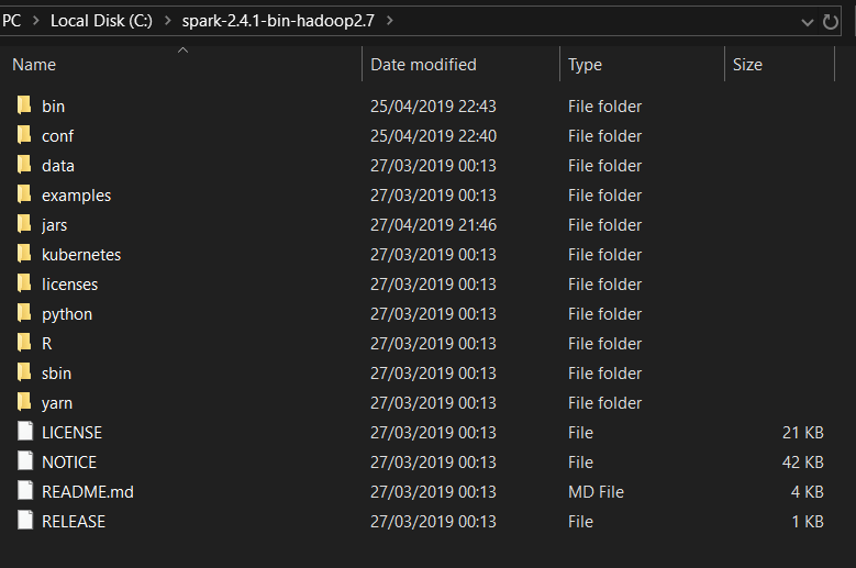
If you have something that looks like this, then you should be in good shape.

Download the Hadoop winutils.exe.

The last step is to download winutils, which is a helper for Hadoop on windows. You can download it from GitHub.

When you have downloaded winutils.exe, you need to put it in a folder called bin inside another folder. I use c:\Hadoop\bin, but as long as winutils.exe is in a folder called bin, you can put it anywhere.

Configure Environment Variables

The final step in configuring Spark is to create some environment variables. I have a script I run from a cmd prompt when I want to use them but can also set system environment variables if you wish. My script looks like this:

SET SPARK_HOME=c:\spark-2.4.1-bin-hadoop2.7
SET HADOOP_HOME=c:\Hadoop
SET JAVA_HOME=C:\Program Files\Java\jre1.8.0_212
SET PATH=%SPARK_HOME%\bin;%HADOOP_HOME%\bin;%JAVA_HOME%\bin;%PATH%

What this script does is set SPARK_HOME to the location of the extracted Spark directory, set JAVA_HOME to the location of the JRE installation, set HADOOP_HOME to the name of the folder that contains the bin directory that winutils.exe is put in. Once the environment variables have been set, I add the bin folder from each to the PATH environment variable.

Testing Apache Spark on Windows

To check everything is set up correctly, check that the JRE is available and the correct version:

In a command window, run Java -version then spark-shell. If you have set up all the environment variables correctly you should see the Spark-shell start. The Spark-shell is a repl that lets you run scala commands to use Spark. Using the repl is a great way to experiment with data as you can read, examine, and process files:
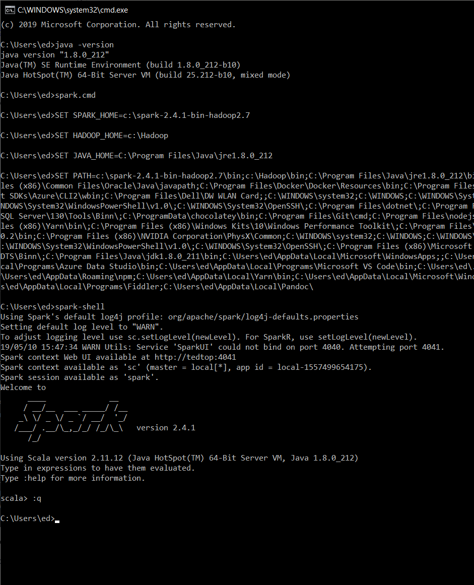
When you are ready to continue, exit Spark-shell by typing :q. You use the spark-shell to check that Spark is working. To run a job later, you use something called spark-submit.

If you can start the Spark-shell, get a prompt and the cool Spark logo, then you should be ready to write a .NET application to use Spark.

Note, you may see a warning that says

NativeCodeLoader: Unable to load native-Hadoop library for your platform… using builtin-java classes where available

It is safe to ignore this; it means that you don’t have Hadoop running on your system. If this is a Windows machine, then that is highly likely.

The .NET Driver

The .NET driver is made up of two parts, and the first part is a Java JAR file which is loaded by Spark and then runs the .NET application. The second part of the .NET driver runs in the process and acts as a proxy between the .NET code and .NET Java classes (from the JAR file) which then translate the requests into Java requests in the Java VM which hosts Spark.

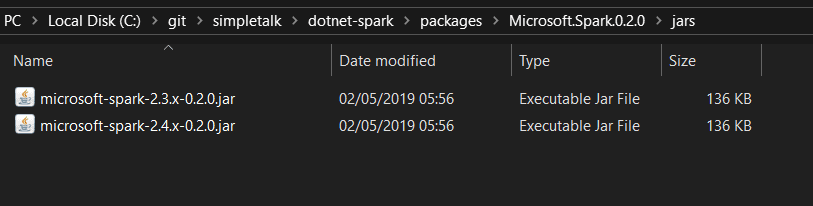
The .NET driver is added to a .NET program using NuGet and ships both the .NET library as well as two Java jars. One jar is for Spark 2.3 and one for Spark 2.4, and you do need to use the correct one on your installed version of Scala.

There was a breaking change to version 0.4 of the .NET driver, so when you use the driver, if you are using version 0.4 or higher then you need to use the package name org.apache.spark.deploy.dotnet and if you are on version 0.3 or less you should use org.apache.spark.deploy, note the extra dotnet at the end.

Your First Apache Spark Program

The .NET driver is compiled as .NET standard so you can use either the Windows .NET runtime or .NET core to create a Spark program. In this example, you will create a new .NET runtime (4.6) console application:
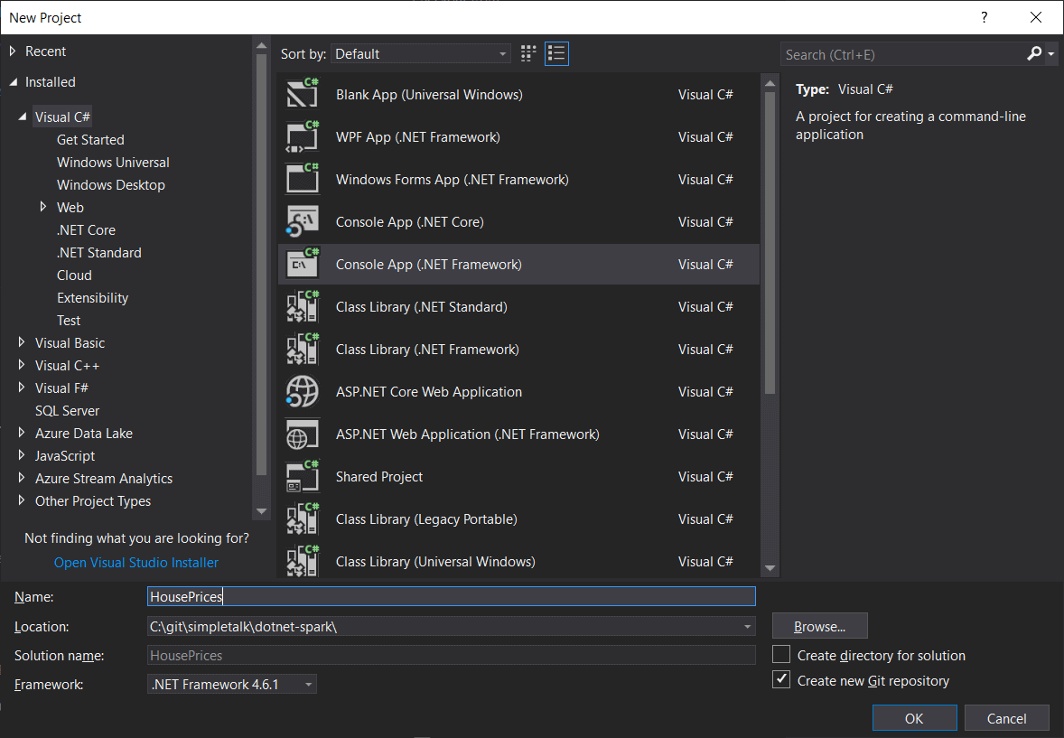
You will then add the .NET Spark driver from NuGet:
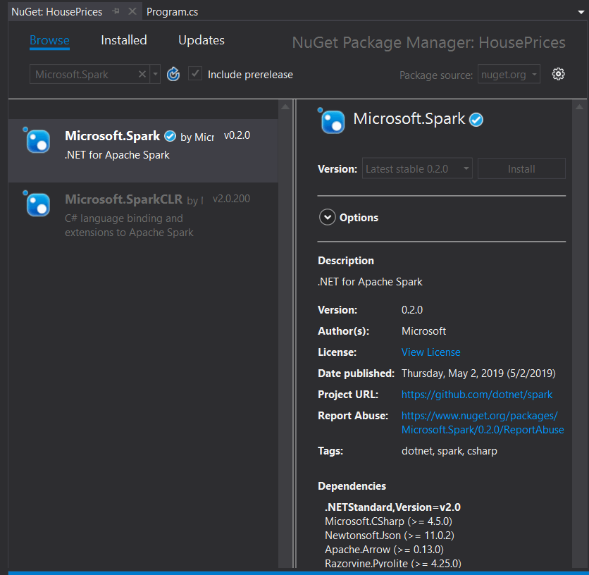
Select Microsoft.Spark. There was also an older implementation from Microsoft called Microsoft.SparkCLR but that has been superseded, so make sure you use the correct one. For this example, use Spark version 2.4.1 and the 0.2.0 NuGet package – these have been tested and work together.

When you add the NuGet package to the project, you should see in the packages folder the two Java jar’s which you will need later:
Execute Your First Program

For the first program, you will download a CSV from the UK government website which has all of the prices for houses sold in the last year. If the file URL has changed, then you can get to it from here after and searching “current month as CSV file”.

The program will read this file, sum the total cost of houses sold this month, and then display the results:

using System;
using System.Linq;
using Microsoft.Spark.Sql;
namespace HousePrices
{
    class Program
    {
        static void Main(string[] args)
        {
            var Spark = SparkSession
                           .Builder()
                           .GetOrCreate();
            var dataFrame = Spark.Read().Csv(args[0]);
            dataFrame.PrintSchema();
            dataFrame.Show();
            var sumDataFrame = dataFrame.Select(Functions.Sum(dataFrame.Col("_c1")));
            var sum = sumDataFrame.Collect().FirstOrDefault().GetAs<Double>(0);
            Console.WriteLine($"SUM: {sum}");
        }
    }
}

The first thing to do is to either use the sample project and build the project or create your own project and build it so you get an executable that you can call from Spark.

First, take a look at this code:

var Spark = SparkSession
      .Builder()
      .GetOrCreate();

Here you create the Spark session. The Spark session enables communication back with the .NET java code and through to Spark.

Next review:

var dataFrame = Spark.Read().Csv(args[0]);
            dataFrame.PrintSchema();
            dataFrame.Show();

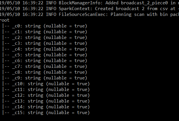
Here the Spark session created above reads from a CSV file. Pass in the path to the CSV on the command line (args[0]). (I realise that you should validate if it exists.) Once the file has been read, the code will print out the schema and show the first 20 records.

Finally look at this code::

var sumDataFrame = dataFrame.Select(Functions.Sum(dataFrame.Col("_c1")));
       var sum = sumDataFrame.Collect().FirstOrDefault().GetAs<Double>(0);
       Console.WriteLine($"SUM: {sum}");

This will use the Sum function against the _c1 column (the price column), it will then select it into a new DataFrame (sumDataFrame) and then it iterates through the rows of the DataFrame. It selects the first row and then retrieves the value of the 0’th column and prints out the results.

To run this, instead of just pushing F5 in Visual Studio, you need to first run Spark and tell it to load the .NET driver and pass onto the .NET driver the name of the program to execute.

You will need these details to run the .NET app:

Type

Name

Value

Environment Variable

JAVA_HOME

Path to JRE install such as C:\Program Files\Java\jre1.8.0_212

Environment Variable

HADOOP_HOME

Path to the folder that contains a bin folder with winutils.exe inside such as c:\Hadoop

Environment Variable

SPARK_HOME

The folder you extracted the contents of the downloaded spark (note that the file downloaded is a tar then gzipped file, so you need to un-gzip then un-tar the file)

The driver package name


For 0.3 and less the driver package is org.apache.spark.deploy and for 0.4 and greater it is org.apache.spark.deploy.dotnet

The full path to the built .net executable


I created my project in c:\git\simpletalk\dotnet\HousePrices so my full path is c:\git\simpletalk\dotet-spark\HousePrices\HousePrices\bin\Debug\HousePrices.exe

The full path to the jars that are included in the Microsoft.Spark NuGet package


Because I created my solution in c:\git\simpletalk\dotnet, my path is C:\git\simpletalk\dotet-spark\HousePrices\packages\Microsoft.Spark.0.2.0\jars\Microsoft-spark-2.4.x-0.2.0.jar
(Note it is the full path including the name of the jar, not the path to where the jars are located) If your NuGet package is version 0.0.3 or something else then the name of the jar will be more like: packages\Microsoft.Spark.0.3.0\jars\Microsoft-spark-2.4.x-0.3.0.jar – every change to the NuGet package will cause this version to change.

The full path to the downloaded house prices csv


In my example it is c:\users\ed\Downloads\pp-monthly-update-new-version.csv

In a command prompt that has these environment variables set, run the next command. (If you still have the spark-shell session open in your command prompt, close it using :q).

spark-submit --class org.apache.spark.deploy.DotnetRunner --master local "C:\git\simpletalk\dotet-spark\HousePrices\packages\Microsoft.Spark.0.2.0\jars\Microsoft-spark-2.4.x-0.2.0.jar" "c:\git\simpletalk\dotet-spark\HousePrices\HousePrices\bin\Debug\HousePrices.exe" "c:\users\ed\Downloads\pp-monthly-update-new-version.csv"

If your executable isn’t called HousePrices.exe, then replace that with the name of your program. When you build in Visual Studio, the output window should show the full path to your built executable. If you aren’t called “ed” then change the path to the CSV file, and if you decided to use Spark 2.3 rather than Spark 2.4, then change the version of the jar.

The Scala code looks in the current working directory and any child directories underneath it to find HousePrices.exe. To see how it does that, you can look at the function resolveDotnetExecutable. You can change the directory in your command prompt to your Visual Studio output directory and run it from there or be more specific in your command line.

Note also that the version of the jar increases with each version of Spark, and because the version is part of the filename, I used 0.3.0 for this article, but new versions are released quite regularly:

Spark-submit –class org.apache.spark.deploy.DotnetRunner --master local PathToMicrosoftSparkJar PathToYourProgram.exe PathToYourCsvFile.CSV

If you run the command line successfully you should see:
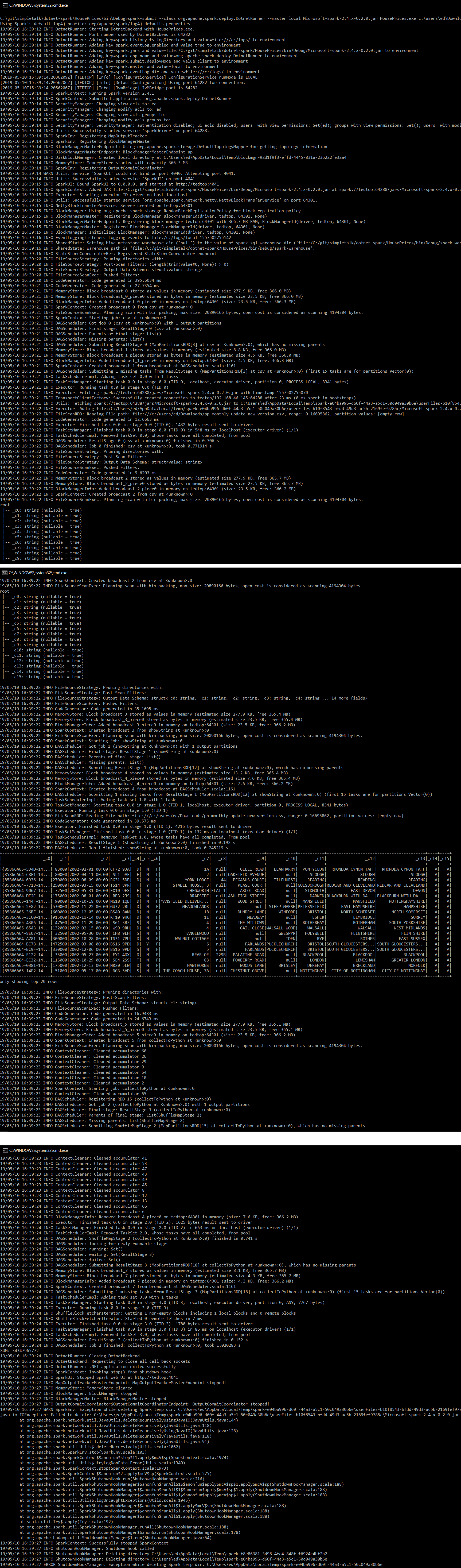
The interesting parts are the schema from dataFrame.PrintSchema():
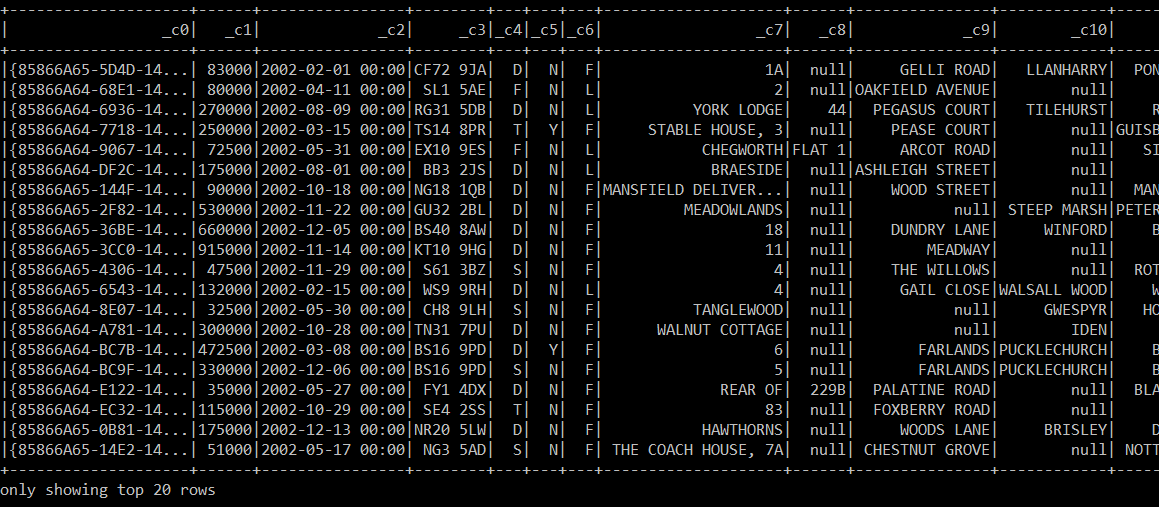
The first twenty rows from dataFrame.Show():
Finally, the results of the Sum:

You may get a lot of Java IO exceptions such as:
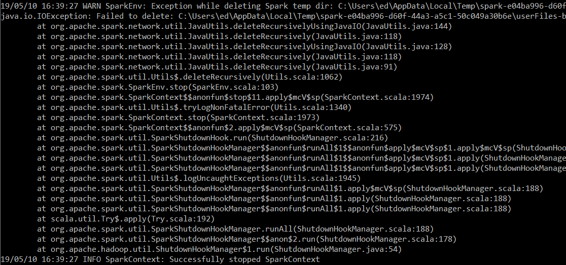
To stop these, in your Spark folder there is a conf directory. In the conf directory, you will have a log4j.properties file add these lines to the end of the file:

log4j.logger.org.apache.spark.util.ShutdownHookManager=OFF
log4j.logger.org.apache.spark.SparkEnv=ERROR

If you don’t have a log4j.properties you should have a log4j.properties.template, copy it to log4j.properties.

A Larger Example

The first example was very basic, and the file doesn’t contain column header, so they are set to _c0, _c1 etc. which isn’t ideal. Also, the output from PrintSchema shows that every column is a string.

The first this to do is to get Spark to infer the schema from the csv file, which you do by adding the option inferSchema when reading the csv. Change the line (line 15 in my program):

var dataFrame = Spark.Read().Csv(args[0]);

into:

var dataFrame = Spark.Read().Option("inferSchema", true).Csv(args[0]);

Build your .net application and re-run the spark-submit command line which now causes PrintSchema() to show the actual data types:
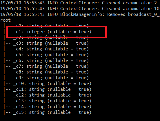
Because you now know the data types, it goes on to break the GetAs<Double>(0) with an Unhandled Exception: System.InvalidCastExceptionL Specified cast is not valid so you also need to change the GetAs<double> to GetAs<long>, from:

var sum = sumDataFrame.Collect().FirstOrDefault().GetAs<Double>(0);

into:

var sum = sumDataFrame.Collect().FirstOrDefault().GetAs<long>(0);

You can test that the program now completes by building in Visual Studio and re-running the spark-submit command line.

It would be good to have the correct column headers rather than _c0, to do this, read the data frame and then re-read the data frame passing in the headers – this doesn’t cause the data to be re-read or re-processed, so it is efficient. If you use this program which reads the data frame, prints the schema and then converts the data frame to a data frame with headers and re-prints the schema, you should see the original _c* column names and the corrected column names:

using System;
using System.Linq;
using Microsoft.Spark.Sql;
namespace HousePrices
{
    class Program
    {
        static void Main(string[] args)
        {
            var Spark = SparkSession
                           .Builder()
                           .GetOrCreate();
            var dataFrame = Spark.Read().Option("inferSchema", true).Csv(args[0]);
            dataFrame.PrintSchema();
            dataFrame.Show();
            dataFrame = dataFrame.ToDF("file_guid", "price", "date_str", "post_code", "property_type", "old_new", "duration", "paon", "saon", "street", "locality", "town", "district", "county", "ppd_Category_type", "record_type");
            dataFrame.PrintSchema();
        }
    }
}

Build your .net application and then re-run your spark-submit command line and you should see the correct column names:

Going further, you can use the column names to filter the data. KENSINGTON AND CHELSEA is a beautiful part of London, see how much houses in that area cost to buy:

using System;
using Microsoft.Spark.Sql;
namespace HousePrices
{
    class Program
    {
        static void Main(string[] args)
        {
            var Spark = SparkSession
                           .Builder()
                           .GetOrCreate();
            var dataFrame = Spark.Read().Option("inferSchema", true).Csv(args[0]);
            
            dataFrame = dataFrame.ToDF("file_guid", "price", "date_str", "post_code", "property_type", "old_new", "duration", "paon", "saon", "street", "locality", "town", "district", "county", "ppd_Category_type", "record_type");
            
            dataFrame = dataFrame.Where("district = 'KENSINGTON AND CHELSEA'");
            Console.WriteLine($"There are {dataFrame.Count()} properties in KENSINGTON AND CHELSEA");
            dataFrame.Show();
            
        }
    }
}

Build the .net application and run the spark-submit command line and you should see something like:

In case you are struggling with the amount of output, you can hide the Info messages by going back to the log4j.properties file located in the extracted spark directory and the conf folder inside that. Change the line:

log4j.rootCategory=INFO, console

into:

log4j.rootCategory=WARN, console

You will see warnings and output but not all the info messages. I would say it is generally better to leave the info messages on, so you get used to what is normal and learn some of the terminology that spark uses.

This new program runs quickly, but Spark is great for processing large files. It’s time to do something a little bit more complicated. First, download the entire history of the price paid data. Download the Single File or the complete Price Paid Transaction Data as a CSV file, currently here.

You can then change the program, so instead of just filtering, it filters and then groups by year and gets a count of how many properties sold per year and the average selling price. One of the features of Spark is that you can use the methods found in Scala, Python, R, or .NET or you can write SQL.

The date must be an actual date, but even with the inferSchema option set to true, it’s still a string rather than an exact date. To correct this, add an extra column to the data set which is the date cast to an actual date:

dataFrame = dataFrame.WithColumn("date", dataFrame.Col("date_str").Cast("date"));

If you build this and then run the spark-submit command line, you should see the extra column:

using System;
using Microsoft.Spark.Sql;
namespace HousePrices
{
    class Program
    {
        static void Main(string[] args)
        {
            var Spark = SparkSession
                           .Builder()
                           .GetOrCreate();
            var dataFrame = Spark.Read().Option("inferSchema", true).Csv(args[0]);
            dataFrame = dataFrame.ToDF("file_guid", "price", "date_str", "post_code", "property_type", "old_new", "duration", "paon", "saon", "street", "locality", "town", "district", "county", "ppd_Category_type", "record_type");
            dataFrame = dataFrame.WithColumn("date", dataFrame.Col("date_str").Cast("date"));
            dataFrame.Show();
        }
    }
}

To query the data using SQL syntax rather than just using .Net methods as shown up to until now, you can save the DataFrame as a view. This makes it available to be queried:

dataFrame.CreateTempView("ppd");

You can then query the view from SQL:

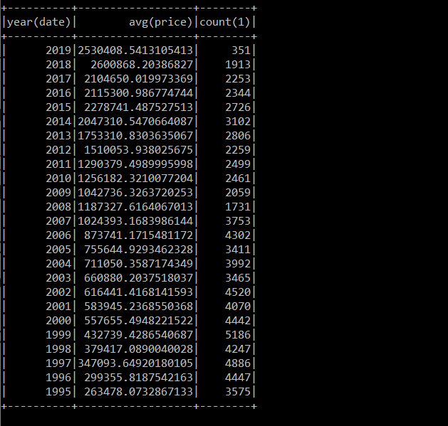
Spark.Sql("select year(date), avg(price), count(*) from ppd group by year(date)").OrderBy(Functions.Year(dataFrame.Col("date")).Desc()).Show(100);

This runs the SQL query

select year(date), avg(price), count(*) from ppd group by year(date)

It then orders the results by date descending and shows the last 100 years (the data only goes back to 1995 so you won’t see 100 years of data).

using System;
using Microsoft.Spark.Sql;
namespace HousePrices
{
    class Program
    {
        static void Main(string[] args)
        {
            var Spark = SparkSession
                           .Builder()
                           .GetOrCreate();
            var dataFrame = Spark.Read().Option("inferSchema", true).Csv(args[0]);
            dataFrame = dataFrame.ToDF("file_guid", "price", "date_str", "post_code", "property_type", "old_new", "duration", "paon", "saon", "street", "locality", "town", "district", "county", "ppd_Category_type", "record_type");
            dataFrame = dataFrame.WithColumn("date", dataFrame.Col("date_str").Cast("date"));
            dataFrame.CreateTempView("ppd");
            
            var result = Spark.Sql("select year(date), avg(price), count(*) from ppd group by year(date)").OrderBy(Functions.Year(dataFrame.Col("date")).Desc());
            result.Show(100);
        }
    }
}

You can then run this against the full dataset:

spark-submit --class org.apache.spark.deploy.DotnetRunner --master local[8] Microsoft-spark-2.4.x-0.2.0.jar HousePrices.exe c:\users\ed\Downloads\pp-complete.csv

You can also change how many cores the processing takes. Instead of --master local which uses one single core by itself, use --master local[8] or whatever number of cores you have on a machine. If you have lots of cores, use them.

When I ran this on my laptop with eight cores, it took 1 minute 45 seconds to complete, and the average house price in that area is about 2.5 million pounds:
Conclusion

Using .NET for Apache Spark brings the full power of Spark to .NET developers who are more comfortable writing C# or F# than Scala, Python, R or Java. It also doesn’t matter whether you are running Linux or Windows for your development.

Source Code

I have included a working copy of the final version of the application on GitHub. In the git repo, there are .NET Framework and core versions of the solution. If you use the .NET core version, then executing the program is the same except instead of HousePrices.exe, you need to have dotnet HousePrices-core.dll before the path to the CSV file:

spark-submit --class org.apache.spark.deploy.DotnetRunner --master local PathTo\Microsoft-spark-2.4.x-0.2.0.jar dotnet PathTo\HousePrices-Core.dll c:\users\ed\Downloads\pp-monthly-update-new-version.csv

References

https://spark.apache.org/

https://github.com/dotnet/spark

The post Apache Spark for .NET Developers appeared first on Simple Talk.


from Simple Talk https://ift.tt/2MpYqbk
via

Saturday, August 17, 2019

Working with React Components

React is a library gaining traction in the enterprise. For large solutions, it is good to have a set of reusable components. Often, back-end APIs written in C# can feed data to a front-end UI. This is where React comes in; it is the UI layer that presents the information to the user. The React library then renders markup using React components. React shops can reuse components to maintain consistent branding across a large suite. This reduces code duplication and increases team velocity. In this take, I’ll delve into working with React components and what it means for .NET developers.

React can live outside Visual Studio. For React development, Visual Studio Code or WebStorm are recommended. The canonical way to begin is through Create React App. Be sure to have Node 8.1+ and NPM 5.6+ installed before working with React.

To fire up a React app:

npx create-react-app work-with-react-app

The contents of the new project will be under the work-with-react-app folder. You can test this new project by running npm start in the project folder.

Think of a React component as an abstraction layer. A component encapsulates HTML/CSS/JavaScript in a single module. This makes it easier to conceptualize a complex UI into many components. This enables plug-and-play of many components to gain rich functionality.

The React library prefers component composition over inheritance. Components are often in a hierarchy of components. To use a baseball analogy, a player has a bat, or a glove, or both. In this analogy, think of the player as a parent component that has many children. For example, a player component might hit, and/or catch a ball. This is how React components unlock functionality through a relational hierarchy. The parent component gains functionality simply by increasing its children. Composition has a lot of flexibility, which improves code reusability.

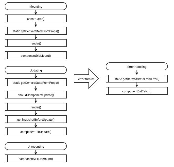
Each React component has its own lifecycle. The component wraps around methods useful for managing state and the component state tells React when it’s time to make updates. The library then finds an optimal way to update the tree hierarchy to reduce repaints. Each lifecycle method can control how updates might occur in the component. To see how React components maintain state, it is essential to understand this lifecycle.

The component lifecycle is broken up into these four phases:

  • Mounting
  • Updating
  • Unmounting
  • Error Handling

With each phase, the component fires a set of lifecycle methods. Error handling only happens when there’s an exception. React treats error handling as a separate and independent phase. Error handling must exclude any logic that belongs in any other phase.

To help visualize the component lifecycle, take a look at this diagram:

To explore each phase, I’ll create a news ticker component. The ticker will update its breaking news every two seconds and show only one headline at a time. To exploit each lifecycle, I’ll freeze, reset, unmount, and throw an error in the component.

Start small by declaring a React component. This can go in a separate file inside the Create React App project. (You can find the completed code for the project here.)

import React from 'react';

class NewsTicker extends React.Component {
}

Mounting

Mounting occurs when the component is created and inserted into the tree hierarchy. This lifecycle executes these methods in the following order:

  • constructor()
  • static getDerivedStateFromProps()
  • render()
  • componentDidMount()

React components have the following method signature in the constructor:

constructor(props)

If the constructor does not initialize state, then the component does not need this. The constructor is called before the component is mounted. For this reason, avoid calling this.setState() but initialize this.state directly. Avoid any side-effects in the constructor that mutate state. Because components subclass React.Component, be sure to call super(props) before any other statement. Else, this.props will be undefined in the constructor which can be problematic.

For the news ticker, put in place a constructor that initializes state. The state will begin with an empty news list and initial index:

constructor(props) {
  super(props);

  this.state = {
    news: [],
    tickerIndex: 0
  };

  this.timer = 0;
}

I’ll skip getDerivedStateFromProps() for now since it is unlikely to be useful during the mounting phase. I’ll come back to this lifecycle method during component updates.

React components have the following method signature when it renders:

render()

This is the only method that is required in a React component. The render() method is pure, meaning it should not mutate component state. Instead, it should use this.props or this.state to render the component. This keeps the component predictable and easier to think about. The render method can return React elements, typically via JSX. For example, <div /> or <NewsTicker />. It can return a string or a number which gets rendered as simple text. Returning a Boolean or null renders nothing because this can unmount components from the hierarchy.
The news ticker will render a list with a single item based on the index:

render() {
  return (
    <ul>
      <li>
        {this.state.news[this.state.tickerIndex % this.state.news.length]}
      </li>
    </ul>
  );
}

The modulus operator allows the news item to iterate as the index increases.

After the component mounts, it calls the following lifecycle method:

componentDidMount()

This is called immediately after the component is inserted into the tree hierarchy. Mutating component state after the initial render goes here. For example, when initiating network requests to fetch back-end data. This method can set and initialize timer intervals. When setting an interval, be sure to clear it in the unmounting phase. Calling this.setState() will trigger another render which goes through the update phase. When using this pattern, be careful as this can cause performance issues. One alternative is to set the initial state through the constructor instead.

The news ticker will grab the latest breaking news with a fetch request. Then, mutate state with the latest data and set up an interval. The interval will update the ticker index as it iterates through each news item.

For example:

async componentDidMount() {
  const payload = await fetch('/news.json');
  const data = await payload.json();

  this.setState({news: data});

  this.timer = setInterval(() => this.setState(
    {tickerIndex: this.state.tickerIndex + 1}), 2000);
}

The interval is set to update the news item every two seconds. Using async/await makes awkward async code more readable. This method returns a void type, but it can also return Promise<void>. Prefixing this method with async makes this return a promise that returns void.

This wraps up the mounting phase. So, what happens when the component mutates state through this.setState()?

Updating

An update occurs when there are changes to the component’s props or state. This re-render lifecycle executes these methods in the following order:

  • static getDerivedStateFromProps()
  • shouldComponentUpdate()
  • render()
  • getSnapShotBeforeUpdate()
  • componentDidUpdate()

React components spend the bulk of their time updating and re-rendering components. This is what makes the components come alive as state mutates through the tree hierarchy.

The getDerivedStateFromProps() lifecycle method has the following signature:

static getDerivedStateFromProps(props, state)

This is called before the render method, both during mounting and updating phases. It returns an object that mutates state or null to change nothing. This method is unlikely to be useful for most use cases. Deriving state from parent components leads to tight coupling, which is hard to understand. A single state change might ripple unpredictable behavior down the component hierarchy. Be sure to look at other alternatives first before going down this path. For example, mutating state can go in componentDidUpdate(). Or, better yet, wrap the component around a state machine like Redux. This method does not have access to the component instance, so it has no side-effects. Extracting pure functions from this method leads to reusable code that can live outside the component. A cleaner way is to abstract state management and unify the tree hierarchy from a single store. This is one problem a library like Redux, for example, attempts to solve.

For the news ticker, reset the component by setting the index back to its initial state. This illustrates how a parent component can alter state with this method.

For example, say there’s a prop to reset state in the component:

static getDerivedStateFromProps(props, state) {
  const {reset} = props;

  if (reset) {
    return {...state, tickerIndex: 0};
  }

  return null;
}

The ES6 spread, for example, …state, sets current values because all I want is to reset the index. Any existing property gets overridden by what’s on the right in the new object. This method is prefixed with static, which means it does not have access to the instance.

The ShouldComponentUpdate() lifecycle method has the following signature:

shouldComponentUpdate(nextProps, nextState)

This is an optimization method to see if the component is affected by the current change in state and props. This method defaults to true and runs right before rendering. For most use cases, it is good enough to rely on the default behavior. Keep in mind preventing rendering can lead to subtle bugs. Consider using a pure component, not a stateless component, for optimization. Pure components do a shallow comparison of props and state to reduce the risk of skipping updates. To create a pure component, subclass React.PureComponent. A stateless component does not subclass any component class. For example, HelloComponent = ({name}) => <p>Hello {name}<p/>. This does not have any lifecycle methods useful for optimization. Avoid deep comparisons with JSON.stringify() because it is inefficient.

Here a freeze prop determines if the news ticker should update:

shouldComponentUpdate(nextProps, nextState) {
  const {freeze} = nextProps;

  if (freeze) {
    console.log('Ticker frozen at: ' +
      nextState.news[nextState.tickerIndex % nextState.news.length]);
    return false;
  }

  return true;
}

The ES6 destructuring assignment is used to grab the freeze prop variable. Then, log nextState.news and block re-render.

The render method executes as it did during the mounting phase. I’ll move on to the next method lifecycle so as not to repeat myself.

The getSnapshotBeforeUpdate() lifecycle method has the following signature:

getSnapshotBeforeUpdate(prevProps, prevState)

This method is called right before the most recent rendered output is committed. This enables the component to snapshot existing information before any changes. Any return value from this method will go as a parameter to componentDidUpdate(). The use case is rare; the one benefit is gaining access to the raw output. For example, capturing what the DOM has before committing changes. React components do a good job at abstracting away the raw DOM. Striping away useful abstractions can be an anti-pattern.

For the news ticker, say I want to grab a snapshot of the current news item. I only want to capture this information when the news list changes after the initial load.

For example:

getSnapshotBeforeUpdate(prevProps, prevState) {
  if (prevState.news.length > 0
    && prevState.news.length !== this.state.news.length) {
    return this.newsRef.current.textContent;
  }

  return null;
}

This needs refs which gains access to the DOM. To make this work, this needs to be set in the constructor():

this.newsRef = React.createRef();

Then, set which DOM element this has access to in render():

<li ref={this.newsRef}>
  …
</li>

The snapshot itself can be of any type. I’m returning a simple string with raw text content.

The last lifecycle method during update has the following signature:

componentDidUpdate(prevProps, prevState, snapshot)

This method is called after all updates are committed. Mutating state here must be wrapped in a condition, else, run the risk of an infinite loop. Keep in mind calling this.setState() causes re-rending which can affect performance. The snapshot parameter comes from the previous lifecycle method. This is the method where the snapshot might be useful for mutating state.

With this lifecycle method, you can check for any news updates from the back-end data. If so, call this.setState() with the latest breaking news. To avoid too many network requests delay this by a factor of two. This method only mutates state when it detects actual changes. To keep it performant, it’s only checking for differences in news length. Also, if there’s a snapshot available then go ahead and log it in the console.

Here’s the method:

async componentDidUpdate(prevProps, prevState, snapshot) {
  if (this.state.tickerIndex % 2 === 0 // delay network calls
    && prevState.news.length === this.state.news.length) {
    const payload = await fetch('/news.json');
    const data = await payload.json();

    if (data.length !== this.state.news.length) {
      console.log('Breaking news update detected.');
      this.setState({news: data});
    }
  }

  if (snapshot !== null) {
    console.log('DOM snapshot before update: ' + snapshot);
  }
}

A modulus delays network calls by a factor of two. Then, it’s checking if both previous and current state are the same to further optimize calls. There is no need to check anything right after a breaking news update.

Unmounting

The unmount lifecycle method has the following signature:

componentWillUnmount()

This is called right before a component is removed from the tree hierarchy and destroyed. Do any necessary cleanup, such as cleaning up intervals created in componentDidMount(). Avoid calling this.setState() because the component will never re-render. In React components, re-mounts are not allowed.

For the news ticker, all I care about is clearing the timer interval. To do this place a log in the console to note an unmount and clear the interval:

componentWillUnmount() {
  console.log('Unmount component.');
  clearInterval(this.timer);
}

Error Handling

React components catch JavaScript errors using error boundaries. This catches errors during render or any other lifecycle method. Because it is a boundary, it can only handle errors in the tree below them. Also, one gotcha is it doesn’t catch asynchronous errors, only synchronous errors.

An error boundary has the following lifecycle methods:

  • static getDerivedStateFromError()
  • componentDidCatch()

The getDerivedStateFromError() method has the following signature:

static getDerivedStateFromError(error)

The lifecycle method is called right after an error is thrown. This receives the error thrown in the tree hierarchy as a parameter. Then, it should return a value to update state in the component. This method is called during render and does not have access to the instance, so side-effects are not permitted.

The next method in the error phase has the following signature:

componentDidCatch(error, info)

This lifecycle method does have access to the instance, so feel free to use this.setState(). This method gets two parameters, error, and info. The error parameter has the actual error thrown. Info is an object containing the component stack, which is where the error got thrown. This method is called during the commit phase, so side-effects are permitted. When it’s not mutating state, it can be useful for logging error information. Keep in mind, when an error is thrown, a fallback UI can render with this.setState(), but this might be deprecated soon. A better approach is to return the new state from getDerivedStateFromError().

For the news ticker, create an error boundary around the NewsTicker component. In the child component, set a prop that throws a bomb so the error boundary can catch it. Once the error boundary diffuses the bomb, it’ll gracefully show a fallback UI.

Here’s the error boundary component:

class ErrorBoundary extends React.Component {
  state = {
    hasBomb: false
  };

  static getDerivedStateFromError(error) {
    return error ? {hasBomb: true} : {hasBomb: false};
  }

  componentDidCatch(error, info) {
    console.log('Caught error: ' + error.message);
    console.log('Component stack - ' + info.componentStack);
  }

  render() {
    if (this.state.hasBomb) {
      // Diffuse bomb with a user-friendly message
      return <p>Unable to show news ticker.</p>;
    }

    return this.props.children;
  }
}

In the child NewsTicker component, change render() so it can throw a bomb:

const {throwBomb} = this.props;

if (throwBomb) {
  throw new Error('Bomb!');
}

Putting It All Together

Both ErrorBoundary and NewsTicker are ready to go into a parent component. The error boundary wraps around the news ticker. The ticker needs props such as reset, freeze, and throw a bomb.

Begin by creating a parent component:

class App extends React.Component {
  render() {
    return <>
    </>;
  }
}
Then declare  state as a class property:
state = {
  reset: false,
  freeze: false,
  throwBomb: false,
  unmount: false
};

The unmount state property allows components to be removed from the tree hierarchy. This will need a set of checkboxes so you can flip between states. Put these between the empty tags in the render method:

<input type={"checkbox"}
  onChange={() => this.setState({reset: !this.state.reset})} />
<label>reset</label>

<input type={"checkbox"}
  onChange={() => this.setState({freeze: !this.state.freeze})} />
<label>freeze</label>

<input type={"checkbox"}
  onChange={() => this.setState({throwBomb: !this.state.throwBomb})} />
<label>throw bomb</label>

<input type={"checkbox"}
  onChange={() => this.setState({unmount: !this.state.unmount})} />
<label>unmount</label>

Then, lay down the components:

{!this.state.unmount && (
  <ErrorBoundary>
    <NewsTicker reset={this.state.reset}
      freeze={this.state.freeze}
      throwBomb={this.state.throwBomb} />
  </ErrorBoundary>
)}

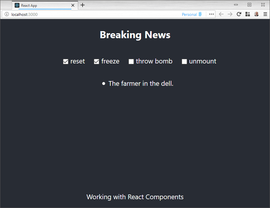
Once you fire this up, it’ll look like this in the browser:

Conclusion

React components are reusable and come in independent modules. They fit within a tree hierarchy using relationships to reuse functionality. Composition is what makes these components more natural to think about. Each component has its own lifecycle that works within the tree’s lifecycle. As components mutate state, the lifecycle is what makes these components come alive.


The post Working with React Components appeared first on Simple Talk.


from Simple Talk https://ift.tt/2yZYeaa
via
Monday, August 12, 2019

Hiding What You Shouldn’t See

Back when I was working on a master’s degree, one of our professors told us a story about a colleague who learned how to navigate the Unix system. She was so thrilled about learning this new skill that, in her exuberance, she stumbled upon some hidden human resource files containing confidential information. Eventually, an administrator realised that the woman had located these files and told her “you can’t do that.” Well, she could and did do that. Even though the files were hidden in the hopes that people wouldn’t find them, they were not secured. Security by obscurity doesn’t work because someone will eventually find what you are trying to hide if they are motivated and put enough effort into it.

On the other hand, there is the problem of showing resources to people when they don’t have rights to them. Nothing is more annoying than clicking on a link and then being told that you do not have permission to view the resource. It would have been better if you hadn’t known about it at all.

In a Windows shop, administrators control what people can do and access by using Active Directory ACLs (access control lists), group membership, and Group Policies. Security in AD can get complicated quickly. To ensure administrators follow the principle of least privilege, proper planning and assigning rights to groups instead of to individual users are essential. I’ve not been an AD administrator, but from a user perspective, it seems to do a good job of both securing and hiding resources.

SQL Server doesn’t always hide what you shouldn’t see. Say an account only has SELECT permission on one table in one database on a server. The account can view all the databases when using SSMS, even those where they can’t connect. After connecting to that one database, they only see the one table in SSMS, but querying other tables returns an error message stating that SELECT permission is denied. A different message appears when attempting to query a nonexistent table. While the specific messages are useful for troubleshooting permissions problems, they give too much information to someone with evil intentions.

Once security has been figured out, it easy for organisations to enable self-service for things like business intelligence or even provisioning virtual machines. It’s essential, however, that the user is not overwhelmed with too many choices. Having too much from which to choose wastes time and can be quite frustrating.

Take a product like SQL Clone, for example, with its new Teams feature. Until the recent 4.0 release, DBAs could only control who could create images and clones, not which ones they could create. For a small shop, that might be good enough. In a bigger team, this might discourage DBAs from allowing self-service to keep someone from creating a clone from an image they shouldn’t see. With the new Teams feature, a DBA has precise control so that developers can only create clones from specific images. This makes self-service more attractive and saves time for everyone involved.

Just hiding what people shouldn’t see never works. Showing them more than they need to see is annoying for the users. Getting security right is a win for both admins and users.


The post Hiding What You Shouldn’t See appeared first on Simple Talk.


from Simple Talk https://ift.tt/2MSENrM
via
Friday, August 9, 2019

Introduction to DevOps: DevOps and the Database

The series so far:

  1. Introduction to DevOps: The Evolving World of Application Delivery
  2. Introduction to DevOps: The Application Delivery Pipeline
  3. Introduction to DevOps: DevOps and the Database

DevOps has been gaining steady ground in the world of application development, with ongoing improvements in delivery processes and the tools needed to support them. For the most part, however, DevOps has focused primarily on the application itself, with databases left to their own devices, despite the integral role they play in supporting many of today’s data-driven workloads.

According to the 2018 Accelerate: State of DevOps report, “database changes are often a major source of risk and delay when performing deployments.” But the report then states that integrating databases into the application delivery process could have a positive impact on continuous delivery. The key, according to the report, is good communication and comprehensive configuration management that incorporates databases. In other words, database changes should be managed in the same way as application changes.

Redgate’s 2019 State of Database DevOps report adds to these findings with their own survey results. According to the report, 77% of the respondents claim that their developers work across both databases and applications, and 75% say that developers build the database deployment scripts. However, 63% acknowledge that DBAs are responsible for deploying database changes to production.

The report also states that the two most significant challenges to integrating database deployments into the DevOps process are “synchronizing application and database changes” and “overcoming different approaches to application and database development.” In contrast, the two biggest reasons for integrating databases into DevOps are “to increase speed of delivery of database changes” and “to free up developers’ time for more added value work.” More importantly, 61% believe that such a move would have a positive impact on regulatory and compliance requirements.

Clearly, integrating database deployments into the DevOps process remains a challenge for many organisations, yet there’s a growing recognition that databases need to be brought into the DevOps fold. And in fact, this is beginning to happen, as more organisations incorporate database deployments into their integration and delivery processes. Not only does this promise to help improve application delivery, but it can also benefit database development itself.

The DevOps Promise

When application and database development efforts are more tightly integrated—with teams working in parallel and sharing a common process—they can release builds that are more consistent and stable, while reducing unnecessary risks and delays. The teams use the same infrastructure to develop and deploy application and database code, making it easier to standardise processes and coordinate efforts.

In a more traditional development environment, database changes can hold up application delivery, impacting productivity and costs. By incorporating databases into DevOps, database deployments can benefit from the established processes, while more tightly integrating database and application development.

A DevOps approach to database development also makes the process more agile and adaptable. Teams implement smaller, more frequent changes as part of a coordinated effort while receiving continuous feedback on the delivery processes and application components. In this way, database development and deployment are no longer disconnected from the larger delivery workflow but become integrated into the process throughout the application lifecycle.

The DevOps Challenge

As good as database DevOps might sound, there’s a good reason that organisations have been slow to jump on board. Transitioning from a siloed-database model to a DevOps-database approach is no small effort.

To begin with, databases were never part of the original DevOps vision. Processes and tools were developed for application code and application deployments, not for the peculiarities of database management. It’s only been recently that databases have been incorporated into DevOps processes in a meaningful way.

Database tools and operations are very specific to database development and management and the environment in which those databases reside. In the early days of DevOps, many viewed the database as existing in a separate world, and both sides of the aisle preferred to keep it that way.

One of the significant differences between application and database deployments comes down to data persistence. With applications, it’s much easier to update or replace code because there’s no data to manage along the way. With databases, however, you can’t simply overwrite schemas or copy changes from one environment to another without pulling the data along with you. Careful consideration must be given to how changes impact existing data and how to preserve that data when changes are made. Otherwise, you risk data loss, integrity issues, or privacy and compliance concerns.

Databases also bring with them size and scalability issues that differ from application code. Implementing schema changes on a massive database in a production environment can be a significant undertaking and lead to performance issues and degraded services. Database changes become even more complicated if the database is being accessed by multiple applications, especially if no single application has exclusive ownership.

Perhaps the biggest hurdle to implementing database DevOps has been a siloed mindset that makes it difficult for various players to come together in a way that makes integration possible. According to the Redgate report, only 22% of the respondents said that their developers and DBAs were “great” at working together effectively as a team, and without a team-focused attitude, an effective DevOps strategy is nearly impossible to implement.

Despite these challenges, however, database DevOps has made important inroads in recent years. DevOps tools now better accommodate databases, and database tools better integrate with DevOps systems. Attitudes, too, are beginning to change as more participants come to understand the value that incorporating databases can offer. Although database DevOps is still a challenge, many teams have now demonstrated that application and database delivery can indeed be a unified effort.

Moving Ahead with Database DevOps

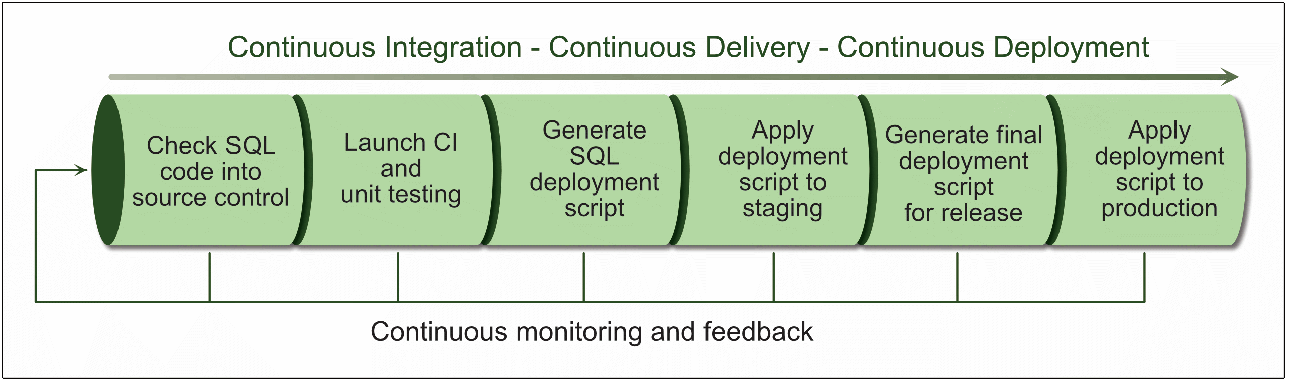
To make DevOps work, the database team must adopt the same principles and technologies as those used by the application team when delivering software. Figure 1 provides an overview of what the database DevOps process might look like when integrated into the application delivery pipeline.

Figure 1. Integrating database deployment into the DevOps process

The first step is to store all database code in source control (also referred to as version control). A source control solution provides the foundation on which all other DevOps operations are based.

With source control, every developer works from the one source of truth, resulting in fewer errors and code conflicts. Source control also tracks who made what changes and when those changes were made. In addition, source control maintains a version history of the files, making it possible to roll back changes to previous versions. Source control also makes it easier to repeatedly build and update a database in different environments, including QA and development.

Database teams should store all their database code in source control. This includes the scripts used to build the databases as well as the migration (change) scripts that modify the database or data. For example, source control should be used for scripts that create, alter, or drop database objects—such as tables, views, roles indexes, functions, or stored procedures—as well as any scripts that select, insert, update, or delete data. The teams should also store static data, such as data used to populate lookup tables, as well as configuration data, when appropriate.

Once all the code and data are in source control, the database deployment operations can be incorporated into the same DevOps continuous integration (CI) and continuous delivery processes used for application deployments. When a developer checks in database code, it triggers an automated build operation that runs alongside the application release process, making it easier to coordinate database and application deployments.

When code is checked into the source control repository, the CI service kicks in and runs a series of commands that carry out such tasks as compiling source code and running unit tests. If a database is part of the deployment, the CI service tests and updates the database—or alerts developers to errors. If problems are discovered, developers can fix them and resubmit the code, which relaunches the CI process.

To incorporate databases into CI, a team might turn to a tool such as Redgate’s SQL Change Automation, which can integrate with any CI server that supports PowerShell. Redgate also provides extensions for CI products such as Jenkins, TeamCity, or Azure DevOps for enabling database integration.

When the CI service processes the SQL code, it produces an artifact that includes the deployment script necessary to update the applicable database objects and static data. The artifact also contains details about the deployment process, including a diff report that shows what has changed in the database. The artifact represents a specific, validated version that can be used as a starting point for the database release process.

At this point, the artifact is deployed against a staging database that is ideally an exact copy of the production database. Here DBAs can verify and confirm the changes to ensure the staging database is production-ready. If necessary, they can also make additional changes. Out of this process, a final deployment script is generated, which can then be passed down the pipeline for deployment against the production database.

Not surprisingly, the exact approach to database delivery is much more involved than what I’ve described here, especially when it comes to migration script versioning, and that process can vary significantly depending on the tools being used and how those tools are configured.

What this does demonstrate is that database DevOps is indeed doable, providing database teams with a process that automates repetitive deployment and testing operations. With DevOps, teams can deliver smaller releases that are easier and faster to deploy, while having in place a consistent, steady mechanism for ongoing database deployments that work in conjunction with application delivery.

Testing and Monitoring

One of the most important aspects of the application delivery pipeline is ongoing testing. Changes to the database should undergo rigorous testing before the release reaches the staging environment. In this way, developers learn of problems quickly and early in the development process. When issues are discovered, they’re immediately alerted so they can check fixes into source control and keep the development effort moving forward.

Developers and DBAs should invest the time necessary to write comprehensive tests that provide for as many scenarios as possible. Many of these tests will be based on frameworks specific to database testing. For example, tSQLt is a popular open-source framework for SQL Server that lets you write unit tests in T-SQL. Regardless of the framework, the goal is the same: to identify as many issues as possible before database changes make it to production.

Unit tests offer your first line of defence against problem SQL code. Because they run when the code changes are checked into source control, they provide the fastest response to possible issues. A unit test is a quick verification of specific functionality or data, such as ensuring that a user-defined function returns the expected result. A unit test should be concise and run quickly, producing a single binary value—either pass or fail.

Also important to the application delivery pipeline is ongoing monitoring, which needs to be as comprehensive as the testing processes themselves. Monitoring can be divided into two broad categories: the feedback loop and system monitoring.

A DevOps application delivery pipeline includes a continuous feedback loop that provides participants with ongoing details about the delivery process. For example, when the CI service notifies developers about problems in their code, those alerts can be considered as part of the feedback loop. Development teams (application and database) should have complete visibility across the entire pipeline. Not only does this help identify issues with the application and database earlier in the delivery cycle, but it also helps to monitor the delivery process itself to find ways to improve and streamline operations.

System monitoring is more typical of what you’d expect of database operations. Once the changes have been deployed to production, you must closely monitor all related systems to check for unexpected issues and ensure that systems are running as they should, before users or data are seriously impacted. To this end, DBAs should monitor database systems for performance and compliance, taking into account regional differences and regulatory requirements. Developers and DBAs alike should have a real-time understanding of issues that might need immediate attention or those that should be addressed in the foreseeable future.

Testing and monitoring also play a critical role in ensuring a database’s overall security. Developers, IT administrators and DBAs must take into account security considerations throughout the entire application lifecycle, addressing issues that range from SQL coding to server security in order to ensure that data is protected at every stage of the application delivery process.

Proper testing and ongoing monitoring can go a long way in helping to enforce these protections. By using source control and automating the delivery process, organisations have a process that is more predictable and easier to manage, while providing an audit trail for tracking potential issues. Database teams still need to ensure proper configurations and secure environments, but an effective DevOps pipeline can also play an important role in your security strategy.

The New Era of Database DevOps

Database DevOps offers the promise of quicker, easier and more secure deployments while bringing application and database development efforts in line with one another. But DevOps is not a one-size-fits-all solution to application delivery, nor is it meant to be a developer-first strategy that leaves DBAs and IT administrators behind.

Developers, DBAs, and operation professionals must work together to implement an application delivery strategy that takes into account the needs of all participants, with the goal of delivering the best applications possible as efficiently as possible in the shortest amount of time. Anything less and your database DevOps efforts are destined to fail.


The post Introduction to DevOps: DevOps and the Database appeared first on Simple Talk.


from Simple Talk https://ift.tt/2YZPIGU
via

Saturday, August 3, 2019

Reporting Services Basics: Parameters

The series so far:

  1. Reporting Services Basics: Overview and Installation
  2. Reporting Services Basics: Creating Your First Report
  3. Reporting Services Basics: Data Sources and Datasets
  4. Reporting Services Basics: Parameters

Adding parameters is one of the essential skills to learn when you are new to SSRS. Parameters give end-users the ability to change the filter of the report on-the-fly. Imagine creating a separate report for every sales year or every department. Even worse, imagine creating a report for every combination of years and departments! With parameters, you can create one report that will work for any combination of these variables.

Starting with the Product List Report

To demonstrate parameters, this article will use the list of products found in the AdventureWorks database. To get started, create a new Report Server Project called Parameters with a shared data source. (See previous articles in this series if you need help understanding how to work with projects, data sources, or datasets.) Add a report named Product List with this embedded dataset:

SELECT P.ProductID, P.Name AS ProductName, P.Color, P.Size, 
   P.ListPrice, PC.Name AS Category, PS.Name AS SubCategory
FROM Production.Product AS P 
JOIN Production.ProductSubcategory AS PS 
  ON PS.ProductSubcategoryID = P.ProductSubcategoryID
JOIN Production.ProductCategory AS PC
  ON PC.ProductCategoryID = PS.ProductCategoryID;

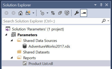
Your Solution Explorer should look like Figure 1.

Figure 1: The Solution Explorer

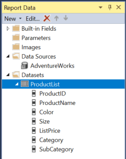
Your Report Data window should look like Figure 2.

Figure 2: The Report Data window

Add a Table control to the report’s canvas and add these fields to the Data row.

  • ProductID
  • ProductName
  • Color
  • Size
  • ListPrice

The table on the report will look like Figure 3.

Figure 3: The table

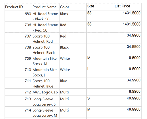
Preview the report to make sure it works at this point. It should look something like Figure 4.

Figure 4: The report in Preview mode

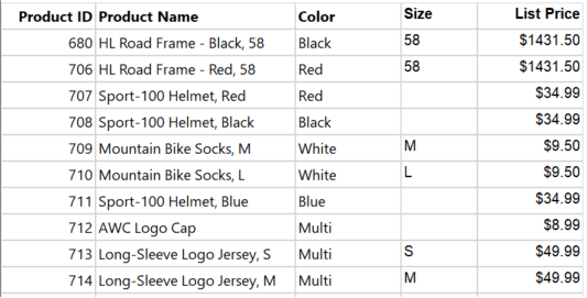
Spend some time formatting the report. This is not required for learning about parameters, but if you are like me, the unformatted report is quite annoying! Your report might look something like Figure 5 when you are done.

Figure 5: The formatted report

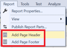
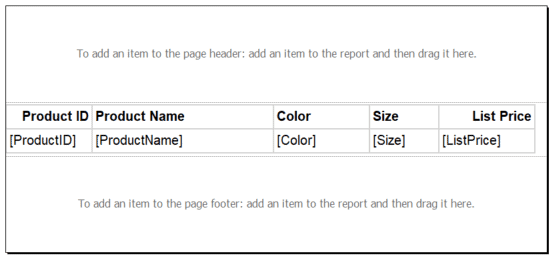
The wizard report from the first article had a header, but you didn’t learn how to add a header to a new report. To do so, make sure that the report is in Design view. Select the report canvas, which makes the Report menu show up in the menu bar. Select Report Add Page Header, as shown in Figure 6. Also, add a page footer.

Figure 6: Add a page header and footer

Move the table so that it is close to the header and the left of the page. Also, drag the top of the footer to the bottom of the table. Drag the right side of the canvas to the table. The canvas should look like Figure 7.

Figure 7: The canvas with header and footer

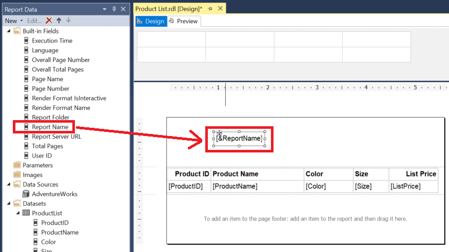
In the Report Data window, expand Built-in Fields. Drag the Report Name field into the page header, as shown in Figure 8.

Figure 8: Drag the Report Name

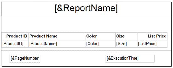
Expand the textbox width to the size of the canvas. Increase the font size to 22 and align the text in the centre. You can also drag Execution Time and Page Number to the footer. (Note that you may need to expand the are under the table where you can temporarily drag the first footer item before adding it to the footer.) The report canvas should now look like Figure 9.

Figure 9: Formatted header and footer

Adding Simple Parameters

SSRS will automatically add parameters to your report when you have variables in the WHERE clause of the query. In this case, you’ll add a parameter to filter on color. Double-click the dataset and change the query to this:

SELECT P.ProductID, P.Name AS ProductName, P.Color, P.Size, 
   P.ListPrice, PC.Name AS Category, PS.Name AS SubCategory
FROM Production.Product AS P 
JOIN Production.ProductSubcategory AS PS 
  ON PS.ProductSubcategoryID = P.ProductSubcategoryID
JOIN Production.ProductCategory AS PC
  ON PC.ProductCategoryID = PS.ProductCategoryID
WHERE P.Color = @color;

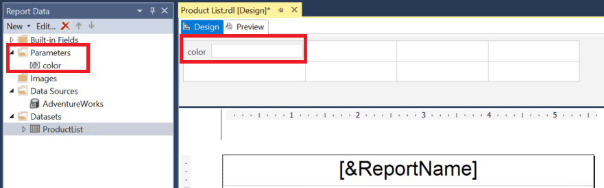
Click OK, and you’ll see the new parameter @color listed in the Parameters folder and the Parameters section of the report canvas, as shown in Figure 10.

Figure 10: The @color parameter

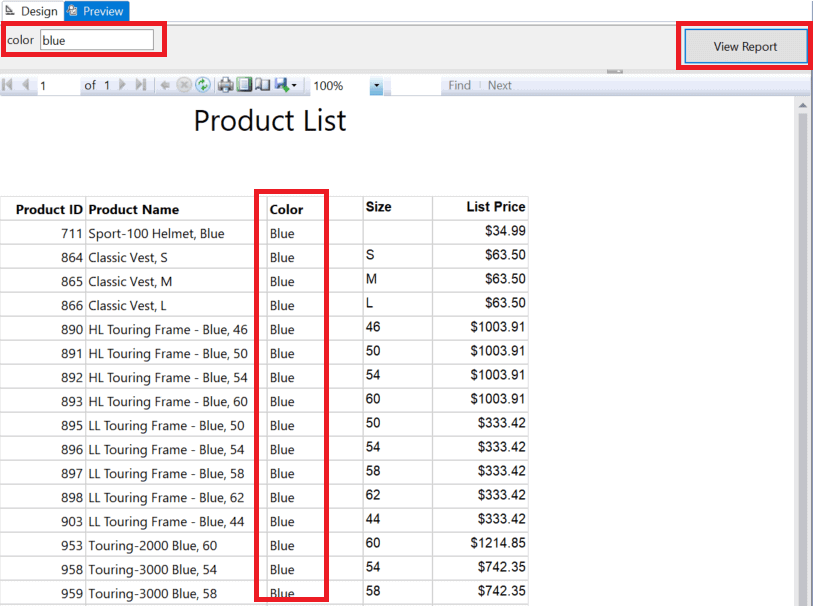
Preview the report. This time, it will not run automatically. Fill in the color “blue” and click View Report. The report should look like Figure 11 with only blue items displayed.

Figure 11: Filtered by blue

Right now, you must type in a valid color to get the report to return products. If you type in “purple,” for example, no products will be returned.

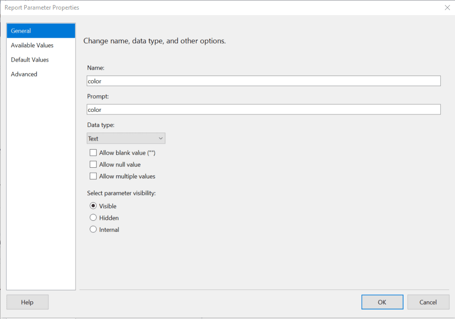
There are quite a few properties you can set to control the behaviour of parameters. You might allow a blank value, for example, or supply a list of values from which to choose. To see the properties, double-click the parameter. The Report Parameter Properties dialogue looks like Figure 12.

Figure 12: The parameter properties

There are a few interesting items to note on the General page. For example, what is the difference between Name and Prompt? The Name refers to the actual name of the parameter that is used in the SQL query. The Prompt is what the user will see. So, you might want to change the “c” in color to uppercase make it more user-friendly.

You can change the Data Type if you must restrict the type of values entered, such as numbers or dates. In fact, if you switch to date, the report will display a date picker control for the parameter when you run the report. There are three other options (Allow blank value, Allow null value, and Allow multiple values) that will be covered later in the article. And, finally, there is the visibility property of the parameter. Here is what each option means:

Visible: The parameter is shown to the end-user who can change the value

Hidden: The end-user is not prompted for the parameter, but the value is typically passed in from a calling report

Internal: The end-user is not prompted and cannot change the value. This might be used for passing in the user id to the server.

There are three more pages to this dialogue. This article will cover Available Values and Default Values. Now, you’ll learn how to provide a list of values for the parameter.

Adding a Parameter List

It can be difficult for the user to remember the valid values for a report, so report developers often provide lists of values from which to choose. To provide a list of colors, follow these steps.

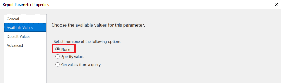
Switch to the parameter’s Available Values page. Currently, the option is set to None, as shown in Figure 13, which means that no list is provided.

Figure 13: The Available Values page

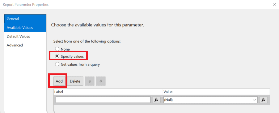
Switch to Specify values and click Add. You’ll now have a space to type in the first value, as shown in Figure 14.

Figure 14: Type in values

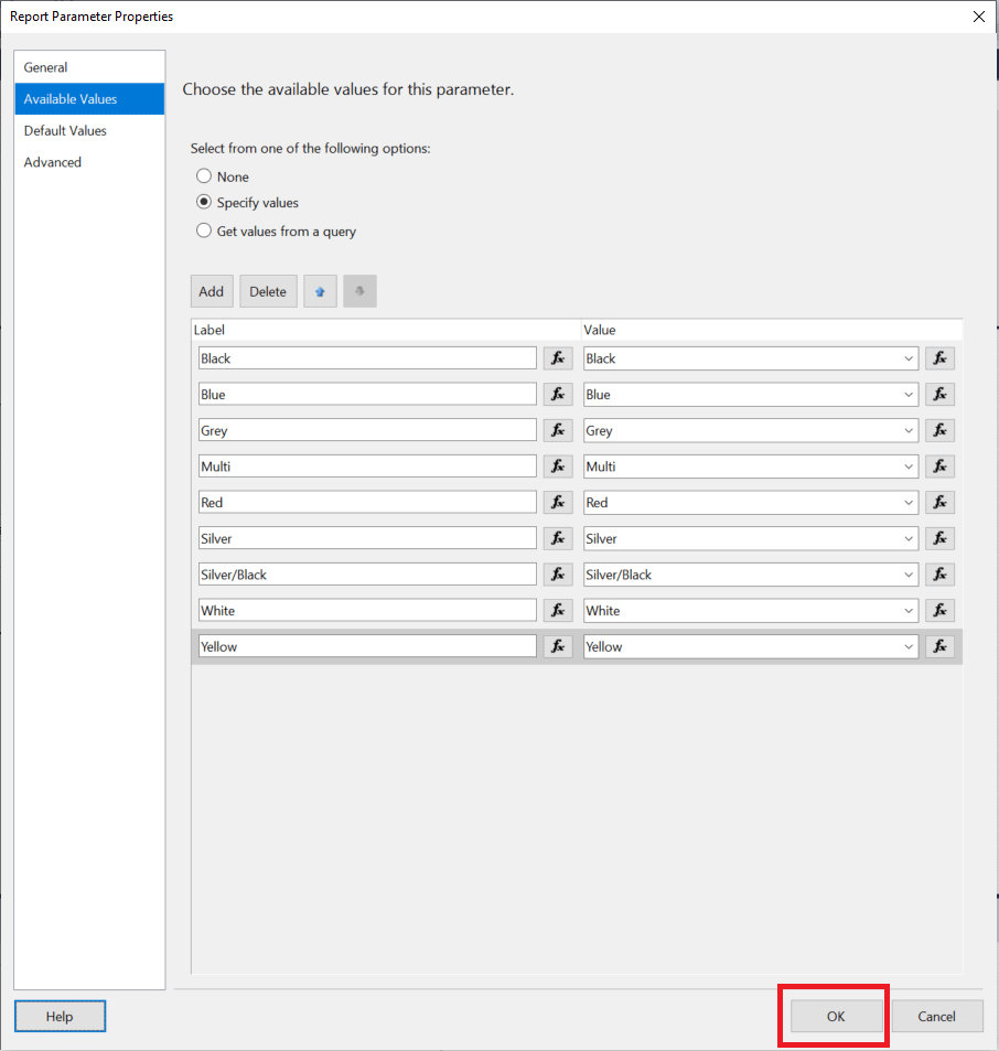
The Label is shown to the end-user, while the Value is passed to the SQL query. In this case, both values are the same. Enter the following list:

  • Black
  • Blue
  • Grey
  • Multi
  • Red
  • Silver
  • Silver/Black
  • White
  • Yellow

The screen should look like Figure 15 when you are done. Click OK to save the list.

Figure 15: The parameter list

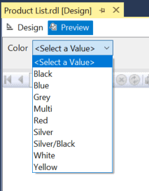
Now when you preview the report, you’ll see a list of colors from which to choose, as shown in Figure 16.

Figure 16: The parameter with the list

Try running the report multiple times, each time with a different color to verify that the report works as expected.

If you are familiar with this data, you’ll know that there are several products with no color (NULL). How can you allow a user to see those products? You’ll learn that next.

Searching for NULL values

You may recall that there is a parameter option to allow NULL (see Figure 12), but to use this option, you must make a change to your query that causes other complications later. It gets messy quickly, so I suggest substituting the NULLs instead.

To get started, add another item to the available values in the Color parameter, N/A for both Value and Label. Double-click the ProductList dataset and change the query to this:

SELECT P.ProductID, P.Name AS ProductName, P.Color, P.Size, 
   P.ListPrice, PC.Name AS Category, PS.Name AS SubCategory
FROM Production.Product AS P 
JOIN Production.ProductSubcategory AS PS 
  ON PS.ProductSubcategoryID = P.ProductSubcategoryID
JOIN Production.ProductCategory AS PC
  ON PC.ProductCategoryID = PS.ProductCategoryID
WHERE COALESCE(P.Color,'N/A') = @color;

When you rerun the report and select N/A, you should see all the items with no color. So far, you are working with a static parameter list. Now, you’ll learn how to create a dynamic list. Note that using a function like COALESCE on a column in the WHERE clause can often cause performance issues.

Using a Query for a Parameter List

What happens if AdventureWorks gets in a new purple or orange product? You would have to manually add those colors to keep the parameter list up to date. Instead, you might want to maintain the list using a query. To do so, switch back to Design view add a new Dataset called Colors to the report with this query that causes the N/A row to show up first.

SELECT DISTINCT COALESCE(Color,'N/A') AS Color, 
        CASE WHEN Color IS NULL THEN 0 ELSE 1 END AS SortOrder
FROM Production.Product AS P 
ORDER BY SortOrder, Color;

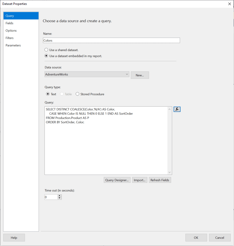
Figure 17 shows how the dataset should look.

Figure 17: The Colors dataset

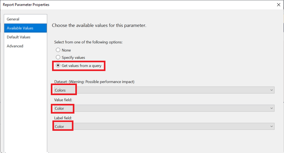
Click OK to create the dataset. Now open the parameter properties again and switch to the Available Values page. Select Get values from a query. Under Dataset, select Colors. In both the Values and Labels field, select Color. The properties should look like Figure 18.

Figure 18: Using a query for the parameter list

Click OK to save the change and be sure to test the report. If you don’t mind modifying a row of the Product table, run this update statement in SSMS or Azure Data Studio.

UPDATE Production.Product 
SET Color = 'Orange'
WHERE ProductID IN (802, 803);

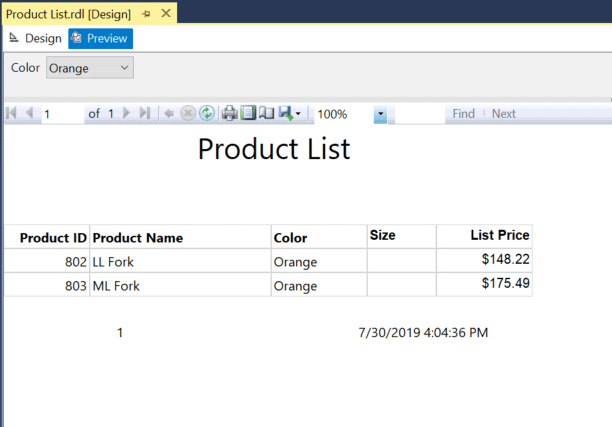
If you rerun the report, you should see Orange in the parameter list and the orange items in the results. Figure 19 shows the report.

Figure 19: The orange items

You might want to give the ability to select multiple items at once. The next section will show you how to do that.

Selecting Multiple Values

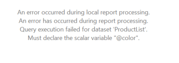
The person running your report might want to see more than one color at a time, maybe even all of them. There is a setting on the General page of the parameter properties (see Figure 12) that allows you to select more than one item. If you do this, however, your query will error, and the report will not run. Figure 20 shows the error message:

Figure 20: The error message after setting Allow multiple values.

The query sent to SQL Server uses = (equal to), but the variable holds a comma-delimited list of values. To fix this issue, you’ll need to modify the ProductList query to this:

SELECT P.ProductID, P.Name AS ProductName, P.Color, P.Size, 
   P.ListPrice, PC.Name AS Category, PS.Name AS SubCategory
FROM Production.Product AS P 
JOIN Production.ProductSubcategory AS PS 
  ON PS.ProductSubcategoryID = P.ProductSubcategoryID
JOIN Production.ProductCategory AS PC
  ON PC.ProductCategoryID = PS.ProductCategoryID
WHERE COALESCE(P.Color,'N/A') IN (@color);

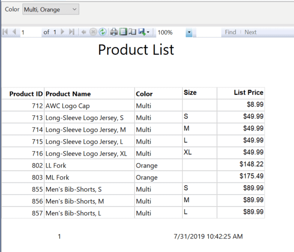
After running, the report should look something like Figure 21 when Multi and Orange are selected.

Figure 21: Selecting multiple values

So far, you have added just one parameter to the report. Many of the reports you run in the future will have more than that. Either the dataset will have multiple predicates in the WHERE clause, or you might also use parameters to control something about how the report looks. In the next section, you’ll learn how to control the value of a textbox in the report with a parameter.

Displaying Parameter Values on the Report

Parameters are the “workhorse” of SSRS. You can do so many things with them. In this section, you’ll learn that you can display the value or label of a parameter in a textbox.

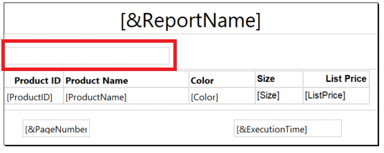
Back in Design view, add a Textbox to the header section of the report. Drag it to the left of the page and expand the width. It should look like Figure 22.

Figure 22: The new Textbox

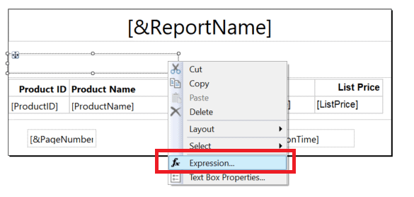
Right-click on the new Textbox and select Expression, as shown in Figure 23.

Figure 23: Select Expression

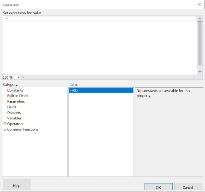
Just about any property in an SSRS report can be controlled with an Expression, i.e., a formula. You’ll learn much more about expressions throughout these articles, but this is a simple example to get you started. Once you select Expression in the menu, the Expression dialogue should pop up, as shown in Figure 24.

Figure 24: The Expression dialogue

Any expression begins with an equal to sign (=) similar to formulas in Excel. The Category area contains dozens of built-in fields and functions that you can use to build these expressions. Change the expression to

="Colors chosen: " +

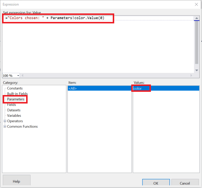
Then, make sure your cursor is to the right of the plus sign (+), click Parameters and double-click color in the Values window, as shown in Figure 25.

Figure 25: The expression

The final expression should be:

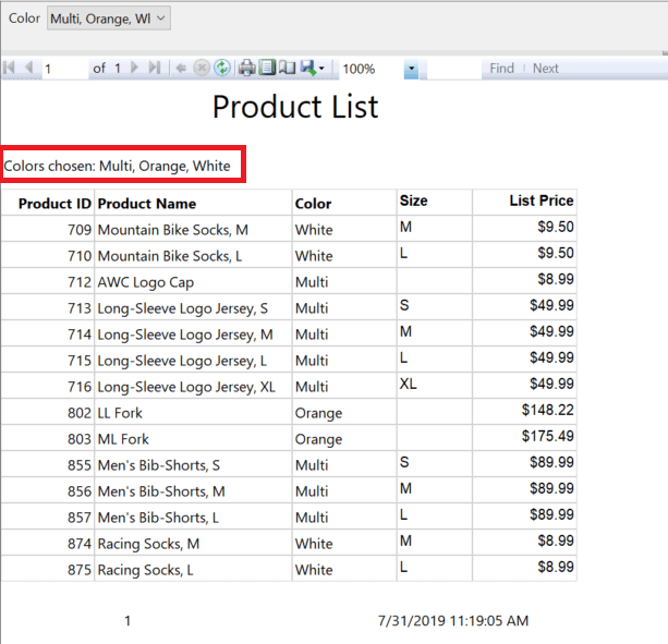
="Colors chosen: " + Parameters!color.Value(0)

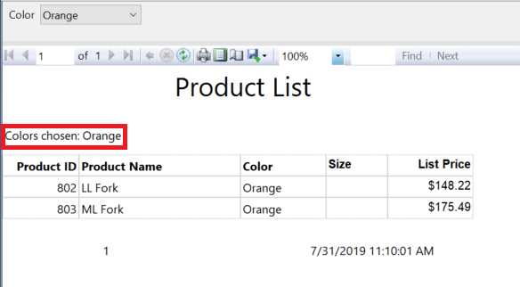
Click OK to save the expression. The Textbox will show <<Expr>> instead of a field name. Run the report but select only one color. The report should look like Figure 26 if you selected Orange. The value you chose is visible on the report.

Figure 26: The parameter value displayed

This works great, but it will only display one item. It’s possible that you are allowing multiple values to be selected. When you select more than one, only the first item is displayed. The reason is that the parameter values are held in an array of strings. Right now, the formula displays the first item in the array.

To display all the chosen values, go back to Design view and bring up the Expression dialogue again. Change the formula to this:

="Colors chosen: " + Join(Parameters!color.Value,", ")

Notice that the index of the array (0) was removed. The Join function builds a string from the array values. Now when you run the report, it will look something like Figure 27.

Figure 27: Displaying multiple values

In this example, the Values and Labels of the parameter are identical. In many cases, they are different. For example, the query might need an ID number while the person running the report might like to see the name. To get around this, change the formula so that the user-friendly label is used instead of the value:

="Colors chosen: " + Join(Parameters!color.Label,", ")

You can also use parameters to change the properties of objects on the report. You’ll learn how to do this next.

Using Parameters to Control Properties

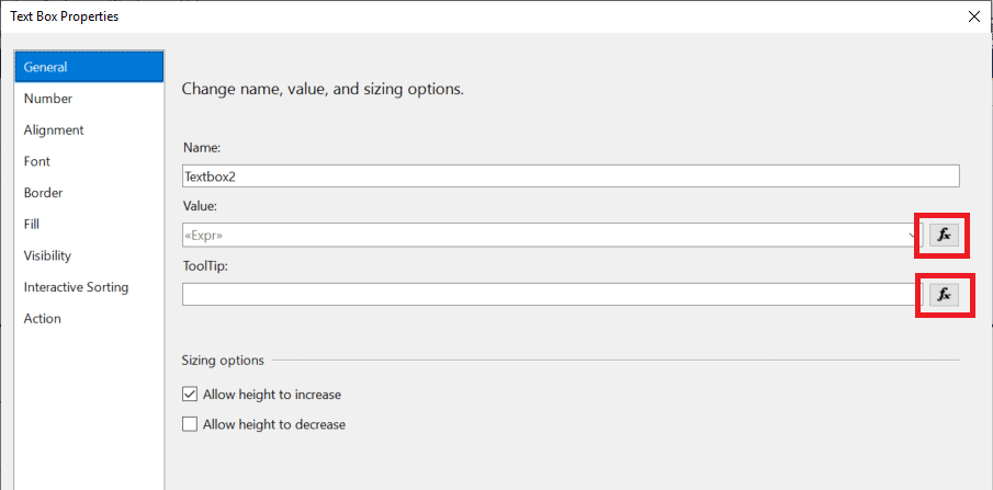
Just about any property in SSRS can be controlled with an expression. If you take a look at the Text Box Properties dialogue of the Textbox you created in the last section, you’ll see the fx symbol next to two properties, as shown in Figure 28.

Figure 28: The fx symbol

Clicking this symbol anywhere you see it brings up the Expression box to control the associated property. Before adding in an expression, cancel out of this dialogue. Create a new parameter called Background by right-clicking the Parameters folder and selecting Add Parameter. Add these values/labels on the Available Values page.

  • Yellow
  • LightBlue
  • Plum

Once all the parameter properties are in place, click OK. You’ll then see the second parameter in the list of parameters. Remember that this one isn’t connected to a dataset query; it will be used to control the background, or fill, color of the Textbox.

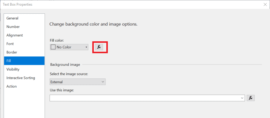
The next step is to connect the parameter to the Textbox. Right-click and select Text Box Properties. Select the Fill page. Click the fx symbol, as shown in Figure 29.

Figure 29: The Fill property

The initial expression is “No Color.” Replace it with this formula:

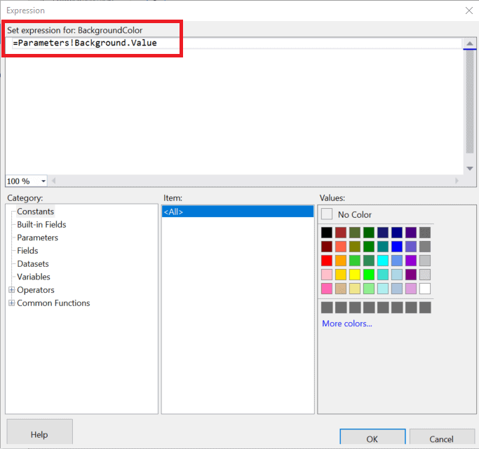
=Parameters!Background.Value

The Expression dialogue should look like Figure 30.

Figure 30: The background expression

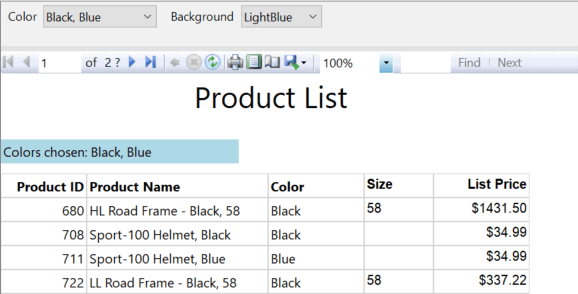
Click OK twice to save the property change. Now, try running the report. If you chose LightBlue, the report should look something like Figure 31.

Figure 31: The textbox with a blue background

This simple example demonstrated how powerful expressions and parameters are. Next, you’ll see how to set default values for parameters.

Using Default Parameters

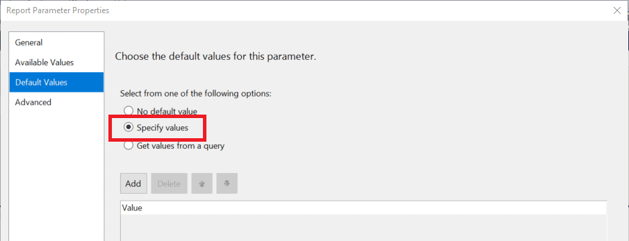
In some cases, the user is likely to select a specific value for a parameter and only rarely change it. To learn how to set up a default value for the parameter, open the properties of the Background parameter. Select the Default Values page and Specify values, as shown in Figure 32.

Figure 32: The Default Values page

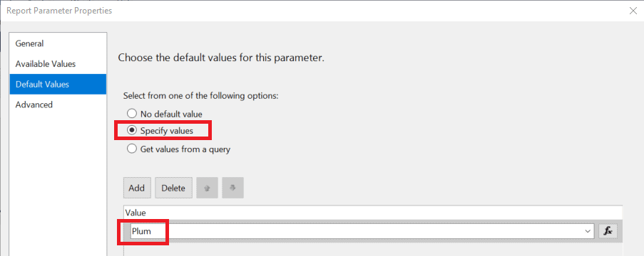
Click Add. Type in your favourite of the three colors, LightBlue, Plum, or Yellow. The property should look like Figure 33. Click OK to save the changes.

Figure 33: Filling in the default value

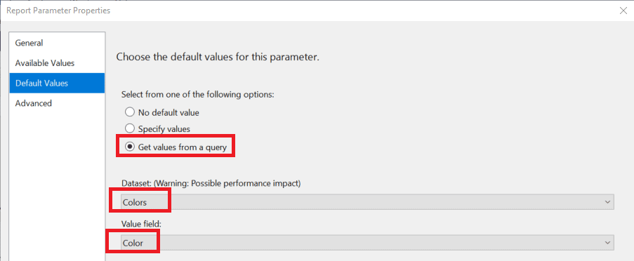
Now when you run the report, the background color will be automatically filled in. You can also get default values from a dataset. Open the Default Values properties of the color parameter. Select Get values from a query. Fill in the Colors Dataset and Color Value field. The properties should look like Figure 34.

Figure 34: The default values from a dataset

In this case, all colors will be selected when you run the report.

One of the most common requests is to make the selection of one parameter filter another one. You’ll learn how to do that next.

Creating Cascading Parameters

Each product belongs to a subcategory, and each subcategory belongs to a category. This is the type of hierarchical relationship that works well when parameters work together with what’s called Cascading Parameters. Figure 35 illustrates how this will work.

Figure 35: The product/category hierarchy

The first step is to modify the ProductList dataset query so that it prompts for the subcategory. Change the query to this:

SELECT P.ProductID, P.Name AS ProductName, P.Color, P.Size, 
   P.ListPrice, PC.Name AS Category, PS.Name AS SubCategory
FROM Production.Product AS P 
JOIN Production.ProductSubcategory AS PS 
  ON PS.ProductSubcategoryID = P.ProductSubcategoryID
JOIN Production.ProductCategory AS PC
  ON PC.ProductCategoryID = PS.ProductCategoryID
WHERE COALESCE(P.Color,'N/A') IN (@color)
  AND P.ProductSubcategoryID = @subcategory;

To make sure that the query works, add the SubCategory and Category fields to the report. Preview the report. Enter subcategory 31. The report should look something like Figure 36.

Figure 36: Filtering with subcategory

At this point, the products are being filtered by subcategory, but the ID must be typed in. To get around this issue, add a new dataset called Subcategory with this query:

SELECT PS.ProductSubcategoryID, PS.Name AS SubcategoryName
FROM Production.ProductSubcategory AS PS
ORDER BY SubcategoryName;

Connect the Subcategory dataset to the subcategory parameter. The Values field should be ProductSubcategoryID, and the Label field should be SubcategoryName. In this case, the query needs the ID while the user needs the name. The Available Values properties should look like Figure 37.

Figure 37: Connect the dataset to the parameter

If you review Figure 35, you’ll see that subcategories should be filtered by category. To do this, change the Subcategory dataset so that it’s filtered by category:

SELECT PS.ProductSubcategoryID, PS.Name AS SubcategoryName
FROM Production.ProductSubcategory AS PS
WHERE PS.ProductCategoryID = @category
ORDER BY SubcategoryName;

You now have four parameters in place. Notice that Category is listed before Subcategory in Figure 38. That’s because you must choose Category before Subcategory. In this parameter area, you can rearrange the parameters by dragging them around. The report will break if Category is not located before Subcategory!

Figure 38: The four parameters

The next logical step is to add a dataset for Category. Use this query:

SELECT PC.ProductCategoryID, PC.Name AS CategoryName
FROM Production.ProductCategory AS PC 
ORDER BY CategoryName;

Connect the dataset to the new Category parameter. You guessed it! The Value field is ProductCategoryID, and the Label field is CategoryName. The Available Values page should look like Figure 39.

Figure 39: The category Available Values

If you did everything correctly, the parameters should look like Figure 40 when you preview the report. Notice that the Subcategory parameter is greyed out until you select a Category.

Figure 40: The Subcategory parameter is not available

When you select a Category, the Subcategory parameter refreshes. For example, if you select Bikes, only the available bike subcategories show up. Figure 41 shows how this looks.

Figure 41: The filtered subcategory

Configuring Cascading Parameters is one of the most challenging things to understand in SSRS. Hopefully, I’ve shown that by breaking the steps down and completing them one at a time, it is doable.

Conclusion

Learning about parameters is critical for SSRS developers. In this article, you learned many ways in which parameters are used, including with a list of available values from a query, multiple selections, defaults, cascading, and more. In the next article, you’ll learn about more features that make SSRS reports dynamic.


The post Reporting Services Basics: Parameters appeared first on Simple Talk.


from Simple Talk https://ift.tt/2Kn1xgK
via