Using Calendars and Dates in Power BI

The series so far:

1. Creating Calculated Columns Using DAX
2. Creating Measures Using DAX
3. Using the DAX Calculate and Values Functions
4. Using the FILTER Function in DAX
5. Cracking DAX – the EARLIER and RANKX Functions
6. Using Calendars and Dates in Power BI

Creating and using a calendar table is pretty straightforward, but this article will explain not just how to create a table, but also why you should want to do this. The article will also answer questions such as: what happens if you have two or more dates in the same table that you want to reference? Or if you have another table which holds information at a different level of granularity? Or if you want to report sales by bank holidays? Read on for how to create a robust data model for handling time-based data!

Loading the Sample Data for this Article

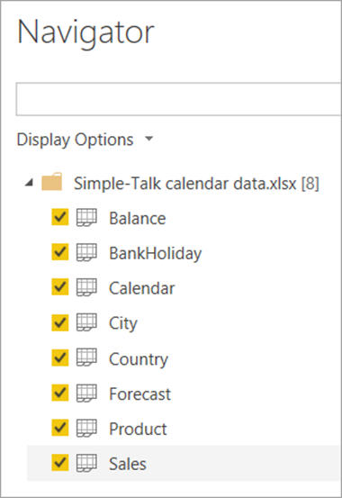
To work through the examples in this article, you’ll need to download the worksheets from this workbook. Tick all of the worksheets when you’re loading data into a new Power BI report:

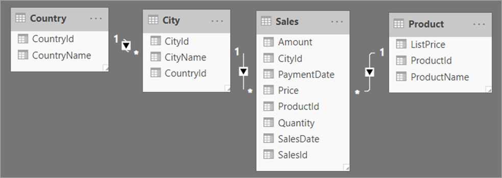
These tables will give you the following data model:

In addition, you should have the following four tables which aren’t linked:

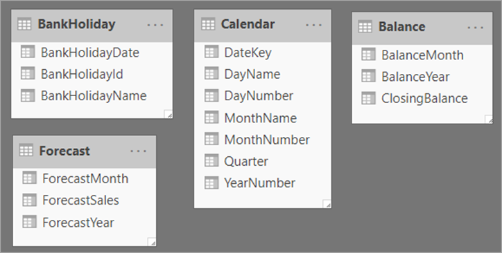
You’ll be using some of these tables in what follows, and some in the next article in the series.

Why Do You Need to Create a Calendar?

When I was first learning Power BI (actually, it was PowerPivot in those days, those many moons ago), I didn’t initially see the point of calendars. After all, Power BI allows you to include fields from date hierarchies which are created automatically for you:

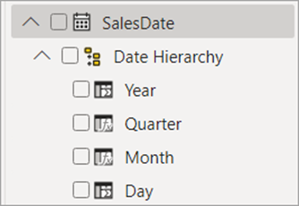
However, having a calendar table gives two big advantages:

• It allows you to aggregate data by non-standard columns (think your company’s financial year, or your timesheet weeks, or the Mayan calendar!).
• It gives you access to all of the wonderful time-intelligence functions in DAX, with names like TOTALYTD and CLOSINGBALANCE. Without a calendar table these won’t work.

Given that most people’s main interest in creating measures in DAX is to compare numbers across time periods, the second point is a bit of a clincher!

The Requirements for a Calendar

What should a calendar table in Power BI look like? Here’s an example:

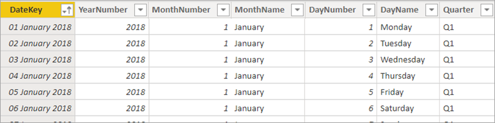
Thus, a calendar table should include one row for each date in your model in which you might be interested. In the example above, the table consists of all the dates in 2018, 2019 and 2020, since this is the lifespan of the transactions in the Sales worksheet. In addition, each date row should have a primary key (a unique field which tells you the date you’re looking at). This doesn’t have to be a date; you could use a separate numeric field instead. However, since dates are stored internally as numbers, I can’t see any reason not to use a date column as your primary key, as above.

Creating a Calendar in DAX

DAX contains a couple of functions which will auto-generate a calendar table for you (this sounds like a good idea, but probably isn’t – read on). One of these is the CALENDARAUTO function. To use this, click on the following tool found on the Modeling tab to create a new table:

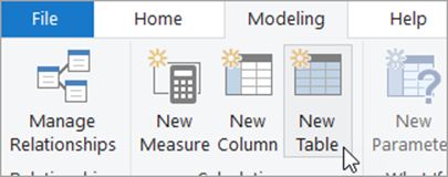
Type in a name for your table. Here I’ve called mine My calendar. Then use the CALENDARAUTO function to say what it will contain:

In this case, just assume that the fiscal year ends in December. You could leave out the argument 12, since December – month 12 – is the default anyway:

My calendar = CALENDARAUTO(12)

When you confirm, you’ll see that this formula Power BI will create a set of dates going from the first date it finds in your data model to the last. In this example the first date is 10^th February 2018 and the last date is 8^th January 2020. Because the financial year ends in December, the function will generate a table containing all the dates for the months January through to December for the years 2018, 2019 and 2020:

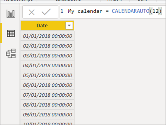
This was all very quick, but also not that useful, as you’re now going to have to add columns giving the year, month, quarter and so on for each date AND then do the same thing for each model that you create.

A variation of the above is the CALENDAR function, which lets you specify a start and end date:

This works in exactly the same way (and suffers from the same drawbacks), but it does at least give you more control over which dates are generated.

Creating a Calendar in Excel

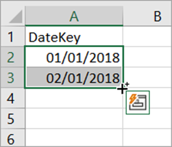
Another way to create a calendar is using an Excel spreadsheet. To do this, type in a column heading and the first couple of dates, and click and drag down using the black cross shown:

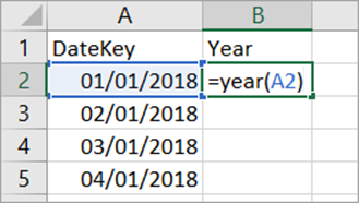
You can now add columns giving the year number, month number, etc. For example, for the year number:

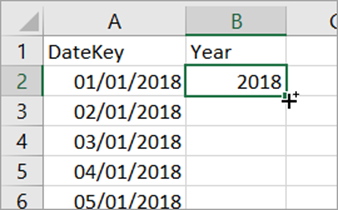
You could then double-click on this black cross to copy this formula down:

Here are some functions that you could use:

• =YEAR(A2) – to get the year number, as above
• =MONTH(A2) – to get the month number, as above
• =TEXT(A2,"mmmm") – to get the month name
• =TEXT(A2,"mm - mmmm") – to get the month number/name
• =DAY(A2) – to get the day number
• =TEXT(A2,"dddd") – to get the day name
• ="Q" & INT((MONTH(A2)+2)/3) – to get the quarter number

You could then save the Excel workbook (possibly pasting the formulae as values first) and use this as a source for your Power BI calendar table.

Creating a Calendar in SQL Server

If you’re using SQL Server, this is probably the best option. Here’s a sample procedure which you can adapt to generate one row for every date in a given range. It doesn’t claim to be that efficient (it uses cursors!), but you’re only going to have to run it once.

CREATE PROC spCreateCalendarTable (
        @StartDate datetime = '20180101',
        @EndDate datetime = '20201231'
) AS
-- create a table of dates for use in Power BI
-- first get rid of any old versions of table
DROP TABLE IF EXISTS tblCalendar
-- create the table of dates
CREATE TABLE tblCalendar(
        DateKey date PRIMARY KEY,
        YearNumber int,
        MonthNumber int,
        [MonthName] varchar(10),
        DayNumber int,
        [DayName] varchar(10),
        [Quarter] char(2)
)
-- now add one date at a time
DECLARE @i int = 0
DECLARE @curdate datetime = @StartDate
WHILE @curdate <= @EndDate
        BEGIN
        -- add a record for this date 
        --(could use FORMAT function if SQL Server 2012 or later)
        INSERT INTO tblCalendar (
                DateKey,
                YearNumber,
                MonthNumber,
                [MonthName],
                DayNumber,
                [DayName],
                [Quarter]
        ) VALUES (
                @curdate,
                Year(@curdate),
                Month(@curdate),
                DateName(m,@curdate),
                Day(@curdate),
                DateName(weekday,@curdate),
                -- the quarter number
                'Q' + CAST(floor((month(@curdate)+2)/3) AS char(1))
        )
        -- increase iteration count and current date
        SET @i += 1
        SET @curdate = DateAdd(day,1,@curdate)
END

Using a Calendar

Once you’ve created a calendar, here’s how to use it. First load it into your data model (in this case, it was loaded with the Excel data), then link it to a date column. Here I’ve assumed that you want to analyse sales by the sale date and not the payment date. Later in this article you’ll learn how to cope with the situation where you have two or more dates in a table.

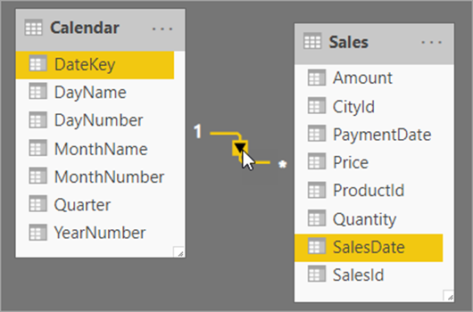
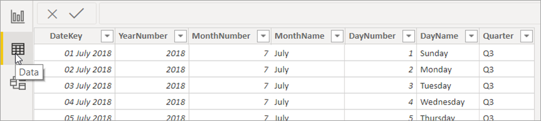
You now need to tell Power BI that the Calendar table is … a calendar table! To do this, make sure you’re looking at the calendar table in Data view:

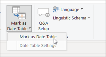
On the Modeling tab, choose to mark this as a calendar table:

Choose the column which uniquely identifies each date, then choose OK:

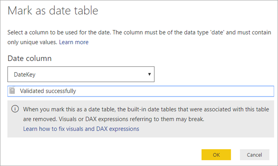
The only problem with all of this is that I’m not convinced it’s necessary! It certainly can’t do any harm, but my understanding is that if you’ve chosen a date column as your primary key, DAX time-intelligence functions will work even if you omit this step.

Fine-tuning Your Calendar Table

To see the Calendar table in action, create a matrix based upon your calendar, using these fields:

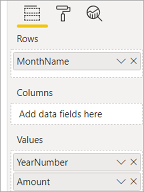
You’ll get something like this:

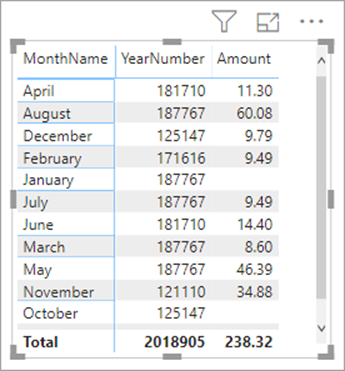
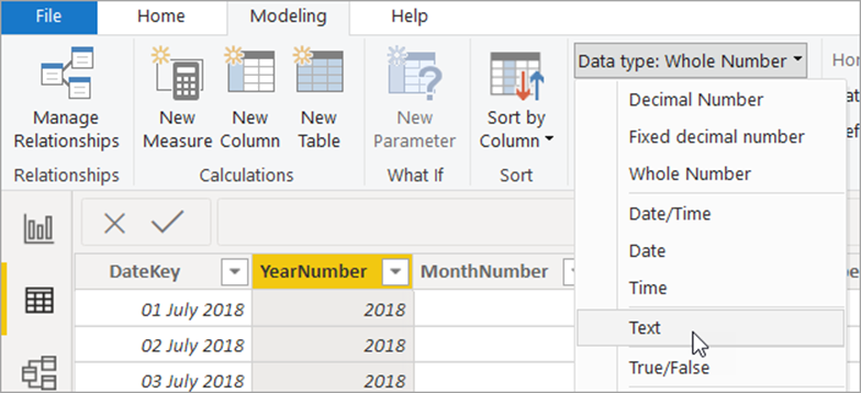
There are two problems here: Power BI has assumed that the year number is an integer which needs summing, and it has also assumed that the month name is text which can be sorted alphabetically. There are other solutions to both problems, but the simplest ones are as follows. First, change the year number to a text column:

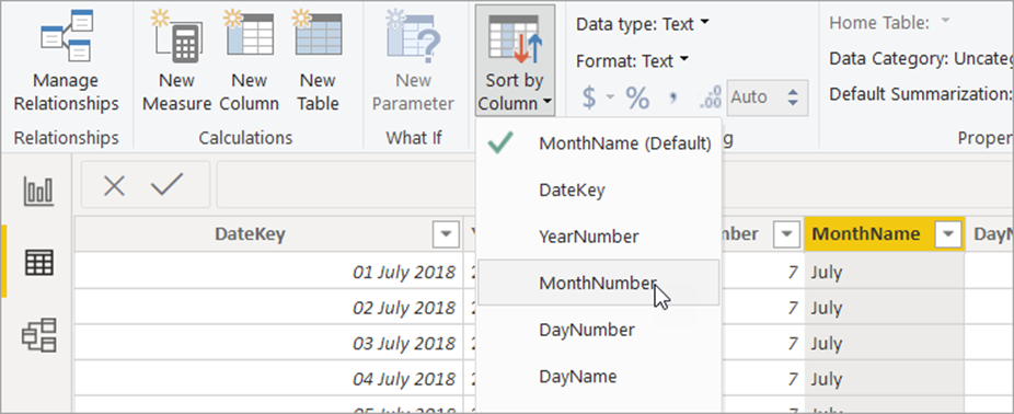
Secondly, with the month name column selected, choose to sort it by month number:

You can now create a matrix with these fields:

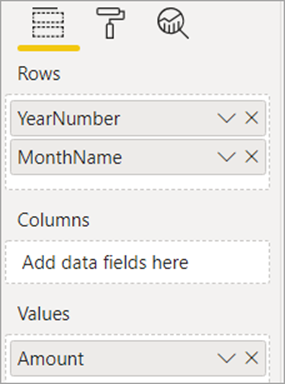
To get this visual:

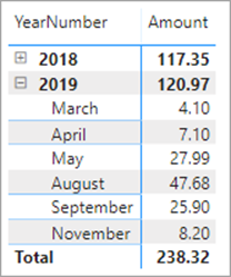
Note that instead of the visual shown above, you may get something like this one:

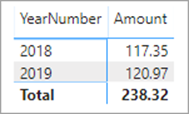
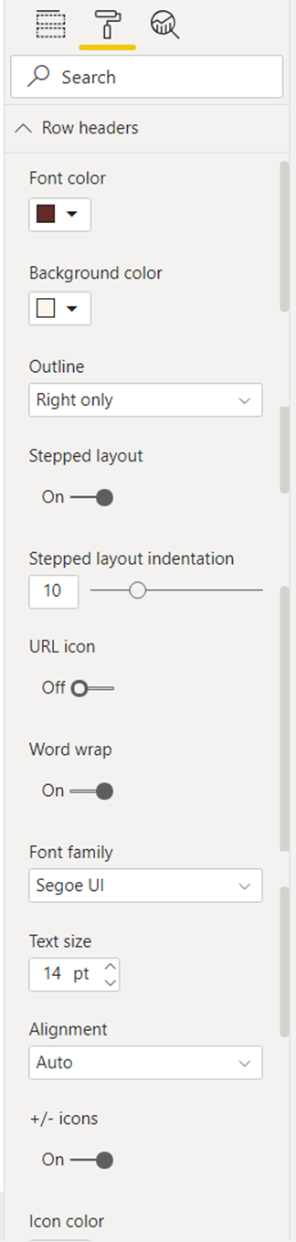
In this case, try finding and setting the +/-icons settings for your matrix in the Row headers card, to enable you to expand and collapse rows:

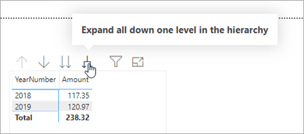
If you don’t have this property, it may be that you’re using an older version of Power BI, in which case, drill down to show all the levels of detail for your matrix:

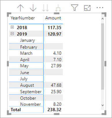
As one final touch, it would be nice to have all of the months appearing, so choose to show items with no date by clicking on the drop arrow next to the MonthName column:

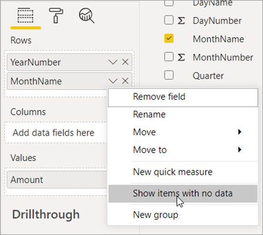
And finally, you’ll see the perfect matrix!

Dealing with Different Levels of Granularity

Suppose now that you want to compare actual and forecast sales which is a common enough requirement. This should be easy – you already have a table of monthly forecasts for sales:

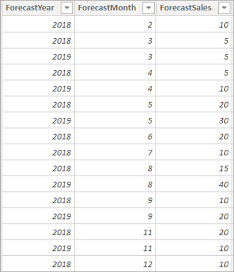
However, these forecasts are by month and the Calendar table is by date. The easiest solution is to create another column which arbitrarily assigns each forecast to the first day of the month in which it occurs:

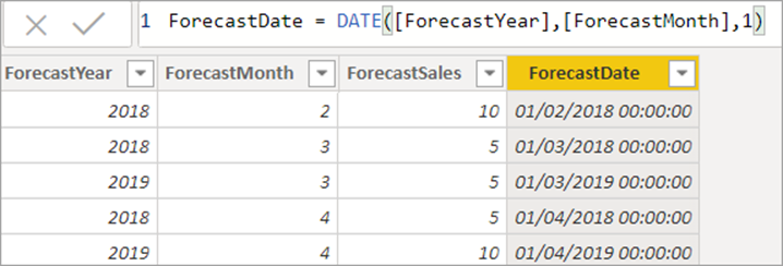
Here’s the formula used:

ForecastDate = DATE([ForecastYear],[ForecastMonth],1)

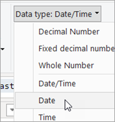
It’s probably a good idea to narrow the data type for this column from Date/Time to just Date:

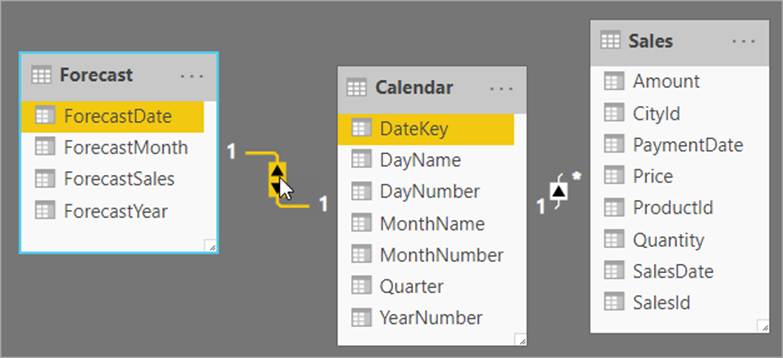
You can now create a relationship between this new forecast date column and the calendar’s date key column:

This will enable you to compare actual and forecast data at any level of granularity down to month:

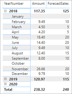
Note that you’ll obviously have to be careful not to drill down to day level, since the forecast sales have been arbitrarily assigned to the first day in each calendar month and the results would be misleading.

Creating New Aggregator Columns (Like Bank Holidays)

Readers outside the UK will need to know that a bank holiday is a day which is treated like a Saturday or Sunday (that is, you don’t have to go to work); there are about 10 of them each year, including Christmas Day, Boxing Day, New Year’s Day, etc. The solution divides sales into working and non-working days where a non-working day is either a Saturday, a Sunday or a bank holiday. To do this, create some new columns in the Calendar table.

Note that you can use this principle to report by any type of date: examples could include periods when you’re offering a discount to customers, timesheet weeks, times of the day when shops are open, etc.

Although you could just create a complicated single column, to make things easier to understand – and to work with – you’ll create three:

1. A column saying whether this is a weekend or not.
2. A column saying whether this is a bank holiday or not.
3. A column combining these two conditions.

To do the first, use the WEEKDAY function, but tweak the second argument so that it returns 6 for Saturday or 7 for Sunday:

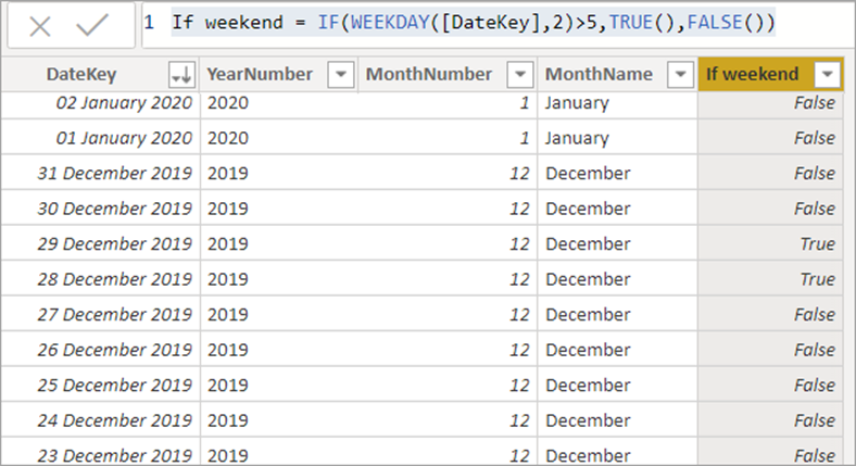
So the full calculated column will be:

If weekend = IF(WEEKDAY([DateKey],2)>5,TRUE(),FALSE())

You could use the shorter form, if you’re comfortable with Boolean algebra!

If weekend = (WEEKDAY([DateKey],2)>5)

This shows, for example, that Christmas Day 2019 was on a Wednesday (that is, 3 days before the next weekend started):

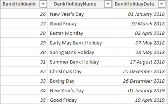
To say whether a day is a bank holiday, for example, you should first create and load a table of bank holidays (or use the one supplied in this article’s Excel workbook):

Now create a one-to-one relationship between the two tables:

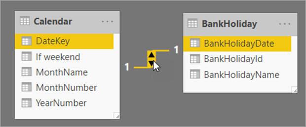
It’s created as one-to-one automatically because the DateKey is unique in the Calendar table, but the BankHolidayDate column is also unique in the bank holidays table too.

You can now create another calculated column in the Calendar table:

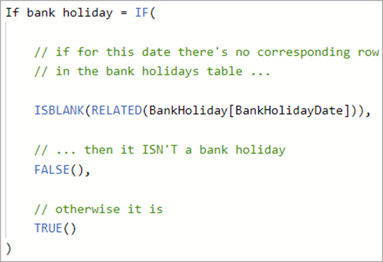
Here’s the code used, for copying:

If bank holiday = IF(
    
    // if for this date there's no corresponding row
    // in the bank holidays table ...
    ISBLANK(RELATED(BankHoliday[BankHolidayDate])),
    // ... then it ISN'T a bank holiday
    FALSE(),
    // otherwise it is
    TRUE()
)

This shows that Christmas Day 2019 was a bank holiday as expected:

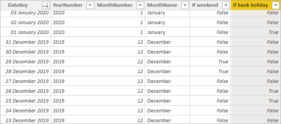
You could now combine the two conditions to get the status of any day:

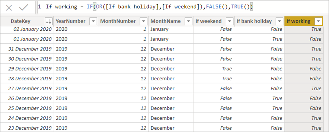
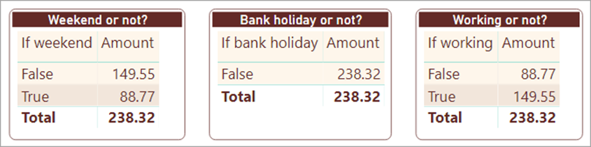
This method will allow you to create reports dividing sales into working and not-working days, although the results aren’t that exciting because as it happens no sales were made on a bank holiday:

Handling Multiple Dates

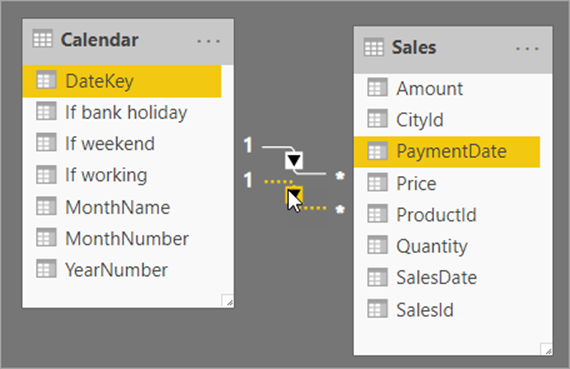
How do you cope when (as is nearly always the case in the real world) a table has two or more dates? For this example, how could you create a visual comparing the month of purchase with the month of payment? There are two ways. One way is to have multiple relationships between the same tables and specify in your measures which one you want to reference:

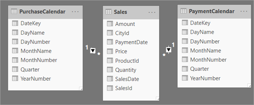
The second method is to use multiple versions of the calendar table:

Which solution you prefer will tell you a bit about what sort of person you are – think of it as a simple personality test. If you’re the sort of person who likes technology for its own sake, you’ll probably prefer the first solution: you’ll like the fact that you’re not storing the calendar table more than once, and you’ll be prepared to sacrifice a bit of ease of use. If on the other hand, you’re the sort of person who likes technology solely as a means to an end, you’ll probably prefer the second solution. Even though it involves holding multiple copies of the calendar table, the resulting model is easier to work with.

The Wise Owl Recommendation

If you’re interested, I prefer the second method (but then I do work for a training company, so by temperament am likely to want to make things as easy to use as possible). However, it doesn’t make you a bad person if you prefer the first method – just different to me.

Both methods are shown under separate headings below. I’ll begin with the multiple table approach since it’s easier to understand and is probably the one that most people will use.

Multiple Tables for Multiple Dates

For this method, start by renaming the first calendar table that you’ve imported. For the model below, the calendar table is linked to the SalesDate column (the date on which a purchase took place), so I’ve renamed the Calendar table to PurchaseCalendar to make it clear what’s going on. I’ve also removed some of the calendar columns to keep the table simple:

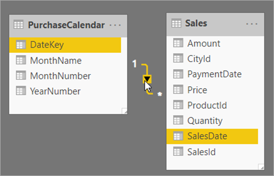
If you have the energy, it would probably be a good idea to rename each of the columns in this table too:

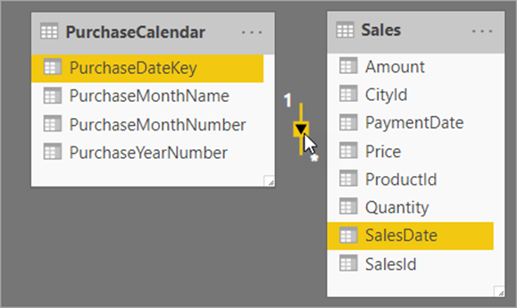
Now choose to load another version of the calendar table using your recent sources (the workbook or database from which you loaded the calendar table will be listed here):

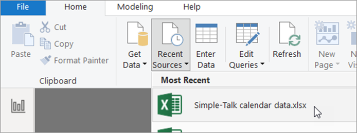
Choose to import another version of the calendar table:

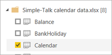
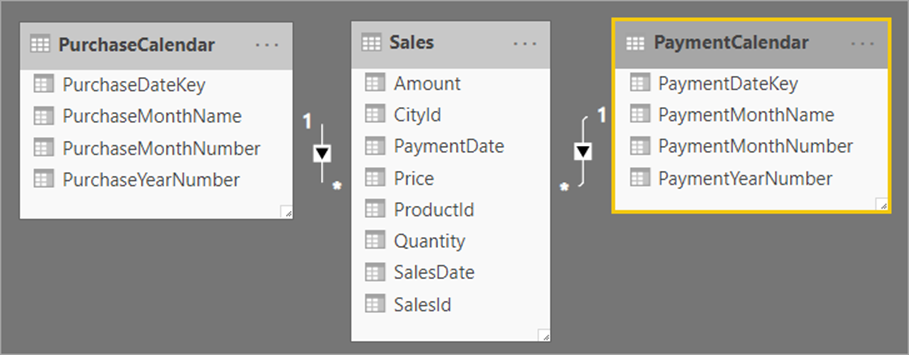
Drag this onto the same layout diagram, and create a relationship between the SalesData table and your recently loaded calendar table, but this time using the PaymentDate column as the link field:

Once again, you could now rename this version of the calendar table (and also rename the columns it contains) to make it clearer what’s what. In this example, I’ve also deleted some columns I don’t want:

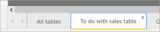
There are two arguments you could make against this approach: that it wastes memory, and that it clutters up your model. Both are true. But it doesn’t waste that much memory. Each table stores about 1,000 dates, which is peanuts in today’s memory terms. It doesn’t have to clutter up your model if you use different tabs like this (one tab for each table containing multiple dates):

Having loaded all of your calendar tables and created the necessary relationships, you could use your model to create a matrix like this, showing the lag between purchases made and payments received:

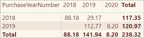
Here’s what the fields for this visual look like:

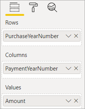
Although the extra table is a bit messy, it does mean that you don’t have to create any additional measures: you can just drag fields into the field well as usual.

Multiple Relationships for Multiple Dates

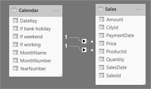
The alternative approach is to load one version of the calendar table, but create a second relationship:

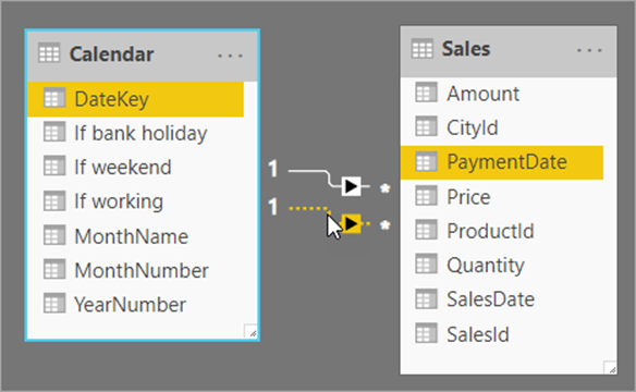
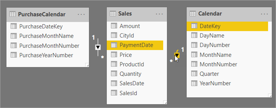
There are now two relationships:

• The active relationship (the one with the solid line) is between the DateKey column in the Calendar table and the SalesDate column in the Sales table
• The selected relationship above (the one with the dotted line) is between the DateKey column in the Calendar table and the PaymentDate column in the Sales table

You can change which is the active relationship by right-clicking on it and choosing to show its properties:

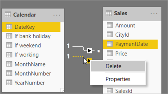
You can then tick the box to make a relationship the active one, but only after making all of the other relationships inactive first, as the following screenshot explains:

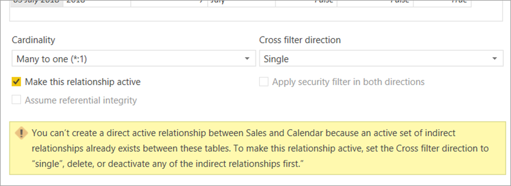
If you’re going to use multiple relationships, it may be a good idea to make all of them inactive. Then you won’t inadvertently create a measure referring to the wrong relationship by mistake:

What you now have to do is to create measures saying for any calculation to which table it should refer. For example, suppose you want to show for each year:

• The total sales made in that year; and
• The total sales paid for in that year.

To do this, create two measures using the USERELATIONSHIP function in each case. Here’s the first one:

Sales by date made = CALCULATE(
    SUM(Sales[Amount]),
    USERELATIONSHIP(
        'Calendar'[DateKey],
        Sales[SalesDate]
    )
)

And here’s the second:

Sales by date paid = CALCULATE(
    SUM(Sales[Amount]),
    USERELATIONSHIP(
        'Calendar'[DateKey],
        Sales[PaymentDate]
    )
)

These measures will allow you to show the required figures:

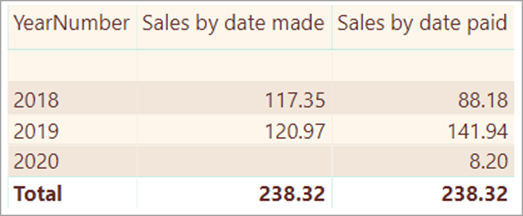
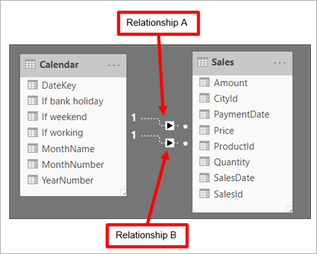
However, there’s no way that I can see to display an aged debtor matrix like the one created for the multiple table approach. It’s also a bit irritating that in the USERELATIONSHIP function that you have to specify the two columns that you’re joining together. It would be better if you could just specify which relationship you’re using. Something like this in fact:

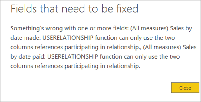
You might also expect that because you are referencing the start column and end column of the relationship, you don’t need the relationship to actually exist, but you’d be wrong, as this error message which appears if you delete the above relationships shows:

And with that mild bit of whingeing, that’s the end of this article!

Conclusion

In this article, you’ve learned how and why you might want to create a calendar table in Power BI, how to use it to report on figures at different levels of granularity, how to add additional aggregator columns to the table and two different ways to cope with the situation where you have more than one date column in the same table. In the next and final article of this series, I’ll show how to use the calendar(s) that you’ve created to show things like year-to-date figures, cross-period comparisons and moving averages.

The post Using Calendars and Dates in Power BI appeared first on Simple Talk.

from Simple Talk https://ift.tt/2ugvQ4s
via

Power BI and Excel

Power BI and Excel are tools so close to each other that Power BI was born inside Excel. Power Query, Power Pivot, Power View, they were all Excel plugins before being united and become Power BI.

The ability to build an ETL, design a model and generate reports and dashboards with great storytelling make Power BI a very powerful tool even beyond the self-service tool which initially was its purpose, but getting closer to an enterprise tool.

However, Excel still has a unique level of flexibility for data analysts. Pivot Tables allow the data analyst to have a view on the model and easily mix measures and dimensions to view a result, even easier then Power BI reports.

When Power BI was created, we easily mistake it as a visualization tool (some people still do this mistake). From that time, power bi has evolved to become very close to an enterprise-level tool.

Nowadays, we have the ability to build powerful ETL architectures building many re-usable dataflows, build models using the ETL as a source and make them re-usable as Datasets published in the portal and create many reports and dashboards from these models.

All these abilities still don’t replace the self-service capability in Excel Pivot Tables. Their flexibility for analysis is unique. So, it’s no surprise that on the way to becoming an enterprise tool Power BI offers Excel connections directly to its datasets.

There are two solutions to make this kind of connection, let’s try.

Analyze in Excel

The first option is the use of the instruction Analyze in Excel. You can find this option on the “…” menu item close to each dataset in the portal.

The idea behind this technique is simple: Power BI is built over the same engine than the tabular model in SSAS. Due to that, you can make a connection to Power BI datasets using Analysis Server as a source.

• When you click Analyse in Excel, the portal downloads to your machine an ODC file. The ODC extension means Office Data Connection, a file with information about how to connect to the dataset.
• Once in Excel, click the Data menu and click the button Existing Connections in the toolbox.

• In the Existing Connections window, click Browse for More button and select the ODC file you just downloaded
• In the Import Data window, select how and where you would like to see the data. For this example, I will use a PivotTable

• In the Import Data window, click Ok

 

The Pivot Table is created inside the worksheet and you will be able to see on the right side the data in your Power BI Dataset. You will also be able to choose the measures and dimensions to build your Pivot Table.

 

Power BI Publisher for Excel

Another option is the user of the Power BI Publisher for Excel. You can download this tool here: https://www.microsoft.com/en-us/download/details.aspx?id=50729

This tool will add a new menu to Excel called Power BI.

• Click on the Power BI menu in Excel
• Click on the button Connect to Data. It will request you to login to Power BI.

• In the window Connect to data in Power BI select the workspace you would like to connect on the dropdown.
• Select if you would like to connect to a Report or to a Dataset on the checkboxes
• Select the name of the Report or Dataset on the 2nd dropdown

 

• Click Connect

A new worksheet will be created with the pivot table, exactly as the previous example.

There are one problem and one advantage. The problem is that you are restricted to connect to classic workspaces. It’s not possible to see the upgraded workspaces. This tool is not updated since 2017 and, according to the official Power BI account on twitter, the upgraded workspaces are still in preview.

The advantage, on the other hand, is that you can also publish data back to power bi, use the option to pin your pivot table in a dashboard.

You can read more details about how to use this tool on this link: https://docs.microsoft.com/en-us/power-bi/publisher-for-excel

Conclusion

The ability to allow self-service BI using Excel puts Power BI closer to the status of enterprise tool, going to one day replace Azure Analysis Services

The post Power BI and Excel appeared first on Simple Talk.

from Simple Talk https://ift.tt/2tny3uw
via

Introduction to Gaps and Islands Analysis

One of the most significant challenges we face when analyzing data is pattern recognition. We seek to find ways in which our data deviates from the norm or conforms to a given norm. The goal is to identify tools that can be used to predict future behavior and make sense out of large volumes of data.

Understanding boundaries and where a pattern begins or ends allows us to draw meaningful conclusions regarding our data. In terms of data, boundaries are more often seen as gaps or islands within any data set. Being able to efficiently locate gaps and islands enables us to use this data to gain meaningful insight into a system. We can identify winning and losing streaks, measure the strength of a system over time, find missing or duplicate data, and a variety of other interesting metrics.

Defining Gaps and Islands

Within a data set, an island of data is any ordered sequence where each row is in close proximity to the rows around it. For some data types and analysis, “close proximity” will mean consecutive. Dates, integers, and letters of the alphabet can be ordered sequentially where two adjacent values will not be able to have additional values in between them.

For example, there are no dates between October 23rd and October 24^th. Similarly, there are no integers between 17 and 18 and no English letters between E and F. For these examples, an island of data could be defined as a sequence of consecutive values. A gap can be defined as a sequence of missing values.

Without rounding or data modification, there are many data types for which “consecutive” has no meaning. Decimals can be ordered, but more can always be placed in between. 12.4 comes before 12.5, but the value 12.45 can be inserted in between. 5:25 occurs after 5:24, but there are many more granular times in between.

In theory, we can use the limits of precision on a data type to define what consecutive means, but this is typically impractical. More realistically, we will consider data points that are close together as sequential for the purposes of analysis. For example, two events that occur at 5:24 and 5:25 may be close enough in proximity that we may wish to highlight them as related. With knowledge of our data and how it works, we can easily make and test rules such as these.

A gap is defined as an absence of data in between islands. Gaps require islands and islands require gaps. For example, if we were evaluating a set of letters of the alphabet and found E, M, and P missing, we could structure a set of islands of this data as follows:

1. A-D
2. F-L
3. N-O
4. Q-Z

The alphabet has been divided up into 4 islands of data. The gaps (all comprised of single letters) are as follows:

1. E
2. M
3. P

A data set with N islands of data must have N-1 gaps in between them. We will typically ignore the edges of the data set and not consider them gaps, even if there are missing values. Testing for specific missing values is a different exercise and not a part of gaps/islands analysis.

A key component to gaps/islands analysis is that the result set is dynamic. Mathematically, we are applying a clustering algorithm to our data, and for any data set, we may end up with a wide variety of results that range anywhere from:

• One giant island with no gaps.
• Lots of small islands surrounded by gaps.
• No islands, and one giant gap (an empty set).

If the list of gaps or islands is our result set, then its size and contents will vary organically based on the data we apply our analysis to. This provides flexibility and insight that may not be available via more rigid analysis.

Grouping Integers

The simplest example of what gaps and islands are is to create a list of sequential, nonrepeating integers:

When we consider this list, we note the numbers range from 1 to 15 and that there are no missing integers. These fifteen integers comprise one big island with zero gaps. Let’s remove some of the numbers from the data set above:

We have removed the numbers 3, 7, 8, and 13 from the list. If we were to perform a gaps/islands analysis on this data, we would find the following islands:

1. 1-2
2. 4-6
3. 9-12
4. 14-15

In between those islands would be the following gaps:

1. 3
2. 7-8
3. 13

How do we solve this problem programmatically? We can model this simple data set in SQL Server like this:

CREATE TABLE dbo.integers
    (integer_id INT NOT NULL);
INSERT INTO dbo.integers
    (integer_id)
VALUES
    (1), (2), (4), (5), (6), (9), (10), (11), (12), (14), (15);

One way to identify gaps is to observe the overall row count and compare it to the expected row count, assuming no gaps existed. Consider the following query and results:

SELECT
    integer_id,
    ROW_NUMBER() OVER (ORDER BY integer_id) AS rownum
FROM dbo.integers;

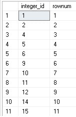
Note that the first column contains what should be an unbroken list of integers, assuming none are missing. The second column contains the row number, also ordered by the integer ID. The result is that we can compare the left column to the right and in any scenario in which the row number falls further behind our ID column, we know another value is missing. The details of what we do with the above numbers as as follows:

1. When integer_id increases by more than rownum, that provides the start of an island.
2. The prior row to the missing values is the end of the previous island.
3. Add 1 to the end of the previous island to obtain the start of the gap.
4. Subtract 1 from the start of the next island to obtain the end of the gap.

We can then use T-SQL to demonstrate how we can crunch the data above into a set of gaps or islands:

WITH CTE_ISLANDS AS (
    SELECT
        integer_id,
        integer_id - ROW_NUMBER() 
            OVER (ORDER BY integer_id) AS island_quantity
    FROM dbo.integers)
SELECT
    MIN(integer_id) AS island_start,
    MAX(integer_id) AS island_end
FROM CTE_ISLANDS
GROUP BY island_quantity;

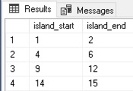
When we execute the above code, we get the following results:

By subtracting the row number from the integer ID, we were able to determine the difference and knew that whenever that number increments, a new gap has been passed in the data set. The ROW_NUMBER window function provides a sequential numbering for our integer list, ranging from 1 to the number of integers in our list (11).

We can calculate gaps using the LEAD window function:

WITH CTE_GAPS AS (
    SELECT
        integer_id,
        LEAD(integer_id) 
            OVER (ORDER BY integer_id) as next_integer
    FROM dbo.integers
)
SELECT
    integer_id + 1 AS gap_start,
    next_integer - 1 AS gap_end
FROM CTE_GAPS
WHERE next_integer <> integer_id + 1;

By comparing the next expected integer ID with the actual next integer ID, we can determine when a gap will start and end. If the current integer is 6 and the next is 9, we immediately know that 7 and 8 are skipped and that there is an upcoming gap comprised of those two numbers.

There are many ways to calculate gaps and islands using a variety of window functions, subqueries, and CTE structures. Our goal in this article is to keep the T-SQL as simple as possible and avoid obfuscated or overly long code.

Managing Duplicates

Consider the following alteration to our data set above:

INSERT INTO dbo.integers
    (integer_id)
VALUES
    (2), (12), (12), (13);

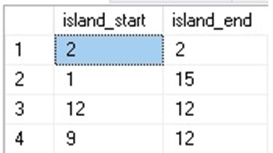
If we run our islands query from earlier, we get the following results:

These results are nonsense, and we can see that the discrepancies introduced by duplicate values need to be dealt with in order to get meaningful results. The ROW_NUMBER window function is useful, but it counts each row as a new value, even if they are the same. Ideally, we would see multiple rows for the same integer as one and the same, and be assigned a single row number, rather than multiple.

The DENSE_RANK window function provides exactly what we are looking for. This function will rank each row in a data set based on the number of distinct values prior to the current row. As a result, duplicates will not impact the results. We can adjust our query from earlier by replacing ROW_NUMBER with DENSE_RANK:

WITH CTE_ISLANDS AS (
    SELECT
        integer_id,
        integer_id - 
        DENSE_RANK() OVER 
           (ORDER BY integer_id) AS island_quantity
    FROM dbo.integers)
SELECT
    MIN(integer_id) AS island_start,
    MAX(integer_id) AS island_end
FROM CTE_ISLANDS
GROUP BY island_quantity;

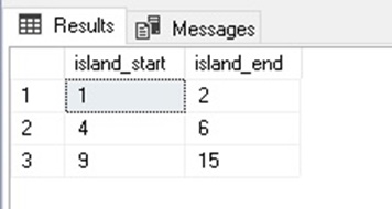
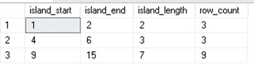
The results are as follows:

After inserting four additional values, the result was to repeat three existing values, as well as introduce a new integer that was previously missing. One less gap means one less island. If we were interested in how many values (duplicate or not) were within each range, we could add that using an added COUNT:

WITH CTE_ISLANDS AS (
    SELECT
        integer_id,
        integer_id - DENSE_RANK() 
            OVER (ORDER BY integer_id) AS island_quantity
    FROM dbo.integers)
SELECT
    MIN(integer_id) AS island_start,
    MAX(integer_id) AS island_end,
    MAX(integer_id) - MIN(integer_id) + 1 AS island_length,
    COUNT(*) AS row_count
FROM CTE_ISLANDS
GROUP BY island_quantity;

The row_count column tells us how many rows are included within each island, including duplicates, which allows us to better understand how prevalent duplicates are within our data set. Island_length was also added as a measure of how many consecutive and unique values exist within each island.

Finding Islands Within Decimal Data Sets

The world is rarely composed of a nice, neat set of consecutive, nonzero, non-NULL integers. Most real data is large, complicated, and ever-changing. Islands can be found within any data set. The key to doing this is establishing rules as to how data relates and is significant. These rules establish two key parameters for analysis:

• Proximity
• Boundaries

Proximity allows us to correlate data to itself, resulting in groups of data. When data transitions from being correlated to uncorrelated, boundaries are created that represent the ends of each island and the ends of its corresponding gaps.

Let’s create a sample data set similar to earlier, but this time using decimals, rather than integers:

CREATE TABLE dbo.decimals
    (decimal_id DECIMAL(14,8) NOT NULL);
INSERT INTO dbo.decimals
    (decimal_id)
VALUES
    (-9999.9999), (-17.9597), (-17.9596), (-17.953), (-17.825), 
    (-5.6), (-5.2), (-4), (-2.68741), (-0.0000001), (0), 
    (1.00056), (2.6), (2.77777), (26.948), (27.1), (17000.17);

This data set has a wide variety of values that includes positive, negative, decimal, and whole numbers. To define islands over this data, we need to establish rules that guide adjacency and create correlated data points that comprise those islands. The simplest and most common rule to apply to data like this would be to consider any two rows where the values of decimal_id are within some arbitrary amount.

For testing, let’s define a rule that all rows where decimal_id is within 1 unit of each other are related and comprise an island. Our T-SQL is going to have to evolve to manage data that is no longer consecutive. From this point on, we will use multiple CTEs to accomplish each task needed to crunch this data:

WITH CTE_DECIMAL_DATA AS (
    SELECT
        decimal_id,
        LAG(decimal_id) OVER 
            (ORDER BY decimal_id) AS previous_decimal_id,
        LEAD(decimal_id) OVER 
            (ORDER BY decimal_id) AS next_decimal_id,
        ROW_NUMBER() OVER 
            (ORDER BY decimals.decimal_id) AS island_location
    FROM dbo.decimals),
CTE_ISLAND_START AS (
    SELECT
        ROW_NUMBER() OVER (ORDER BY decimal_id) AS island_number,
        decimal_id AS island_start_decimal_id,
        island_location AS island_start_location
    FROM CTE_DECIMAL_DATA
    WHERE decimal_id - previous_decimal_id > 1
        OR CTE_DECIMAL_DATA.previous_decimal_id IS NULL),
CTE_ISLAND_END AS (
    SELECT
        ROW_NUMBER() 
             OVER (ORDER BY decimal_id) AS island_number,
        decimal_id AS island_end_decimal_id,
        island_location AS island_end_location
    FROM CTE_DECIMAL_DATA
    WHERE next_decimal_id - decimal_id > 1
        OR CTE_DECIMAL_DATA.next_decimal_id IS NULL)
SELECT
    CTE_ISLAND_START.island_start_decimal_id,
    CTE_ISLAND_END.island_end_decimal_id,
    (SELECT COUNT(*) 
     FROM CTE_DECIMAL_DATA 
     WHERE CTE_DECIMAL_DATA.decimal_id BETWEEN 
        CTE_ISLAND_START.island_start_decimal_id 
        AND CTE_ISLAND_END.island_end_decimal_id) 
     AS island_row_count
FROM CTE_ISLAND_START
INNER JOIN CTE_ISLAND_END
ON CTE_ISLAND_END.island_number = CTE_ISLAND_START.island_number;

This T-SQL can be broken into 4 steps:

1. Collect the data to be processed. In this example, it is in CTE_DECIMAL_DATA.
2. Find all island starting points based on lack of proximity to a previous row. In this example, it is in CTE_ISLAND_START.
3. Find all island ending points based on lack of proximity to a next row. In this example, it is in CTE_ISLAND_END.
4. Join island starting points to island ending points and report on the results.

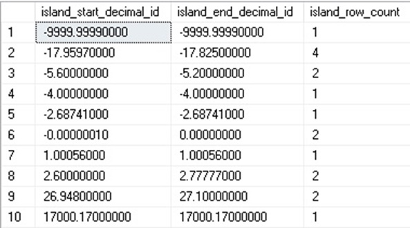
Since the number of island starting points is guaranteed to match ending points, we know that we will get a clean join at the end of our T-SQL. The results of this query are as follows:

Our set of 17 decimals has been crunched down into ten islands containing anywhere from one to four rows. An island can span more than 1 unit if each consecutive row happens to fall within one unit of the next. For example, consider the following number sequence:

1…1.5…2.25…3…4…5…6

Apply our algorithm to these numbers, and we will get a single island with all seven numbers in it as each decimal is within one unit of the next one. What if we add some duplicate values into our table:

INSERT INTO dbo.decimals
    (decimal_id)
VALUES
    (-9999.9999), (-17.825), (0), (27.1);

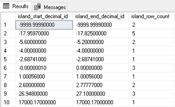
When we run our analysis query, we get the following results:

Our new algorithm protects us against bad/nonsensical data resulting from duplicate values. Either a decimal has a value within one unit of it, or it does not. The count at the end of the query will include any number of contained values, regardless of their frequency. While this T-SQL is longer than what we used previously, we will use it going forward in our analysis for several reasons:

1. Each CTE is relatively simple and easy to understand and modify.
2. We can copy and paste the syntax for other types of data with few modifications.
3. The final join will always be the same for any data type.
4. Adding metrics via subselects, CTEs, or other added queries is easy.

This is a scenario where longer and more explicit code is beneficial and will buy us scalability for future queries we write.

The benefit of this sort of analysis, in general, is that it allows us to crunch together rows of data into groupings based on any metric. While we started with integers and expanded into decimals, we could very easily apply the latest query to any other data type that we dream up.

Finding Islands in Date/Time Data

The most practical application of gaps/islands analysis is to apply it to dates and times. We often want to know if events are related to each other, and one of the top ways they may be related is if they occur near each other in time. Consider some of these scenarios:

• Marketing campaigns send our advertisements regularly. People view and may click on these ads. Were clicks and purchases based on the ads or not?
• A development team manages a variety of servers that support an application. If apps, services, or hardware fails in sequence, were those outages related?
• The CDC tracks search terms, looking for internet searches that involve medical symptoms, such as a runny nose, headache, or muscle pain. The CDC also tracks occurrences of infectious diseases. When are symptom searches and disease incidences close enough to be related?
• When is a stock investment team on a winning streak? How many consecutive trades resulted in more than a specified amount of gains?
• In sports, what qualifies as a winning streak? Can we measure streaks in other metrics, such as ice time in hockey, at-bats in baseball, or shots in basketball? What if we filter by metrics to look for patterns based on details, such as handedness, time of day, location, temperature, and more…?

This is a rabbit hole that can take us down a significant analytics journey. Let’s take our previous query and extend it to time data:

CREATE TABLE dbo.datetimes
    (datetime_data DATETIME2(3) NOT NULL);
INSERT INTO dbo.datetimes
    (datetime_data)
VALUES
    ('7/17/2019 00:05:00.157'), ('7/17/2019 00:07:25.000'), 
    ('7/17/2019 00:30:00.777'), ('7/18/2019 12:00:00.565'), 
    ('7/19/2019 12:00:00.980'), ('7/20/2019 12:00:00.098'),
    ('7/21/2019 12:00:00.332'), ('7/15/2019 21:46:15.197'), 
    ('7/15/2019 21:42:00.000'), ('7/1/2019 14:12:06.674'),      
    ('7/1/2019 14:12:06.986'),  ('7/3/2019 01:11:02.001'), 
    ('7/6/2019 09:58:58.840'), ('7/10/2019 16:33:00.702'), 
    ('7/12/2019 23:19:00.411');

This table contains fifteen datetime values with precision up to 3 decimal places. Let’s say we are looking at software exceptions and want to group together any events that occur close together as potentially related. We decide that any events that occur within 5 minutes of another event are related. Using this single rule, we can modify our T-SQL used for decimals to analyze this data as well:

WITH CTE_DATETIME_DATA AS (
    SELECT
        datetime_data,
        LAG(datetime_data) 
            OVER (ORDER BY datetime_data) AS previous_datetime,
        LEAD(datetime_data) 
            OVER (ORDER BY datetime_data) AS next_datetime,
        ROW_NUMBER() OVER (ORDER BY datetimes.datetime_data) 
        AS island_location 
    FROM dbo.datetimes),
CTE_ISLAND_START AS (
    SELECT
        ROW_NUMBER() OVER (ORDER BY datetime_data) AS island_number,
        datetime_data AS island_start_datetime,
        island_location AS island_start_location
    FROM CTE_DATETIME_DATA
    WHERE DATEDIFF(MINUTE, previous_datetime, datetime_data) > 5
        OR CTE_DATETIME_DATA.previous_datetime IS NULL),
CTE_ISLAND_END AS (
    SELECT
        ROW_NUMBER() 
            OVER (ORDER BY datetime_data) AS island_number,
        datetime_data AS island_end_datetime,
        island_location AS island_end_location
    FROM CTE_DATETIME_DATA
    WHERE DATEDIFF(MINUTE, datetime_data, next_datetime) > 5
        OR CTE_DATETIME_DATA.next_datetime IS NULL)
SELECT
    CTE_ISLAND_START.island_start_datetime,
    CTE_ISLAND_END.island_end_datetime,
    (SELECT COUNT(*) 
     FROM CTE_DATETIME_DATA 
     WHERE CTE_DATETIME_DATA.datetime_data BETWEEN 
        CTE_ISLAND_START.island_start_datetime AND 
        CTE_ISLAND_END.island_end_datetime) 
    AS island_row_count
FROM CTE_ISLAND_START
INNER JOIN CTE_ISLAND_END
ON CTE_ISLAND_END.island_number = CTE_ISLAND_START.island_number;

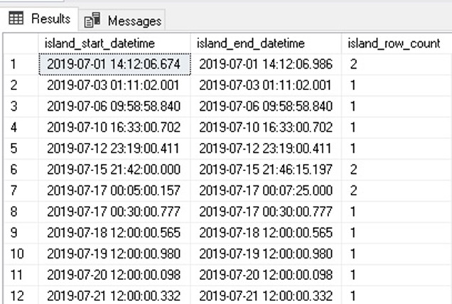
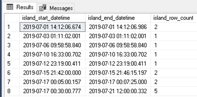
Our syntax is identical to earlier with the sole exception of our island definition. Here, an island boundary is defined by a row in which the previous or next datetime value is more than five minutes away from it. The results are as follows:

The results show pairs of related events, with the rest appearing farther apart than the allotted window of 5 minutes. We note in the results that some times were repeated often, for example, there were four days in a row with events at about 12:00.

Islands analysis specifically is not built to capture these, though if we knew with certainty that these were singular events daily, we could adjust our query to look at islands as defined by events that are a day apart, but at similar times of the day (within a 5 minute rolling window):

WITH CTE_DATETIME_DATA AS (
    SELECT
    datetime_data,
    LAG(datetime_data) 
        OVER (ORDER BY datetime_data) AS previous_datetime,
    LEAD(datetime_data) 
        OVER (ORDER BY datetime_data) AS next_datetime,
    ROW_NUMBER() OVER 
        (ORDER BY datetimes.datetime_data) AS island_location
    FROM dbo.datetimes),
CTE_ISLAND_START AS (
    SELECT
        ROW_NUMBER() 
            OVER (ORDER BY datetime_data) AS island_number,
        datetime_data AS island_start_datetime,
        island_location AS island_start_location
    FROM CTE_DATETIME_DATA
    WHERE DATEDIFF(MINUTE, previous_datetime, datetime_data) > 5 
        AND DATEDIFF(DAY, previous_datetime, datetime_data) <> 1
        OR CTE_DATETIME_DATA.previous_datetime IS NULL),
CTE_ISLAND_END AS (
    SELECT
        ROW_NUMBER() OVER (ORDER BY datetime_data) AS island_number,
        datetime_data AS island_end_datetime,
        island_location AS island_end_location
    FROM CTE_DATETIME_DATA
    WHERE DATEDIFF(MINUTE, datetime_data, next_datetime) > 5 
        AND DATEDIFF(DAY, datetime_data, next_datetime) <> 1
        OR CTE_DATETIME_DATA.next_datetime IS NULL)
SELECT
    CTE_ISLAND_START.island_start_datetime,
    CTE_ISLAND_END.island_end_datetime,
    (SELECT COUNT(*) 
     FROM CTE_DATETIME_DATA 
     WHERE CTE_DATETIME_DATA.datetime_data 
         BETWEEN CTE_ISLAND_START.island_start_datetime AND 
         CTE_ISLAND_END.island_end_datetime) 
     AS island_row_count
FROM CTE_ISLAND_START
INNER JOIN CTE_ISLAND_END
ON CTE_ISLAND_END.island_number = CTE_ISLAND_START.island_number;

This is a far more customized query that will group either by events that are within 5 minutes of each other or those that are a day apart and also within 5 minutes:

The results allow us to focus also on those scenarios where the same alerts occurred day after day at similar times. A query like this shows that we can easily tailor our analysis to unusual scenarios. An island of data is defined by the filters used to determine the starting points and endpoints. These filters can be simple or wildly complex, depending on how detailed our use-cases are.

Conclusion

Gaps and islands analysis allows us to crunch data based on proximity rather than fixed groupings. This provides greater flexibility and the ability to generate result sets that otherwise could be exceptionally challenging to create.

The basic concept of a data island can be extended from integers to other data types, such as strings, decimals, dates, and times. The T-SQL syntax used can be reused for each iteration of our work with only minimal changes to the details of how it works. This allows for maintainable code that can be reliably implemented and reused as needed.

Ultimately, these analytics allow us to group data organically to identify patterns or related events. These insights can be used for monitoring, alerting, or further analytics and decision-making processes.

 

The post Introduction to Gaps and Islands Analysis appeared first on Simple Talk.

from Simple Talk https://ift.tt/39BOaW2
via

Happy New Year’s Resolutions

This has been quite a year, which is why this year’s resolutions are not in October as had been my previous practice. This year for me has been defined by three major things:

1. Knee replacement – Having had one of my hips replaced twice, I figured I had this knocked out cold and would actually get more work done than normal. The doctor made me think it was to be extremely awful, but it actually never was that bad in terms of pain. It did however require a lot more time exercising, and still does. I generally spend 1.5 hours a day at the gym (including 5 mile round trip) every day the gym is open and I am not doing some other physical task, but the aches and pains just take longer to recover from than normal.
2. Book project – I am on the verge of completing my part of a large SQL Server 2019 book, revising 2 chapters and tech editing 10 others. It started way before my surgery in May and has been quite a lot of work that has yet to be completed. It is coming to an end in the near future, and I am definitely ready to do the next thing!
3. Being on program committees – I worked on SQL Saturday Chattanooga, Music City Data, and the PASS Summit; all working with others shaping the data content for these conferences. Some weeks had 3+ hours of meetings, and some extra tasks to do for the upcoming conferences. While it is very hard work, I am really quite proud how these conferences turned out, and the small part I played in that process.

These three ongoing things really highlighted a problem that I have, in that I tend to only work on one thing at a time unless forced. So if I have to work on the book, even if I am caught up at one point in time, I don’t want to write another blog or article.  If deadlines start accumulating, I will certainly start working on that next thing, but then I get stuck on that task, and so forth. On whatever task I have going I get obsessive and start getting up early, staying up late (those do not go together as you get a bit more age on you), and thinking about it all of the time. 

To start this year out, I am going to focus on making one really major life change, that isn’t about diet and exercise. I am going to work on managing my life in a preemptive multitasking manner rather than cooperative multitasking. In cooperative multitasking, the process that has control of the processor must give up control voluntarily. But in preemptive multitasking the algorithm makes sure every task gets a slice of time to work. If you used early versions of Windows you may remember the pain when a task went nuts and held on to the CPU forever, this sort of describes my life. (SQL Server uses cooperative multitasking in its operating system too). Instead of letting one task take over my life, I will try to make sure I have time for everything, and do my best to really use time slices wisely (because I have 3 weeks of vacations already planned, and now that Disney+ is out, I also have plenty of TV to watch as well).

There are plenty of tasks to give time slices to. For this year, we have just started the SQL Saturday Chattanooga process in earnest, and PASS Summit tasks ramp up after the first of the year too. Music City Data work is not far away from kicking off either. I am also scheduled to start working on the 6th edition of my database design book this year (to which I really need to learn more about graph and microservices before I start). What should help this year, is that I won’t be getting my knee replaced again (barring the new one failing, I suppose,) and I am told that my knee should be healed by July!

Recapping last year’s resolutions and making less crazy promises for next

In terms of last year’s resolutions, I did okay. When the year started I did not realize I would be able to get the knee done, and it changed my trajectory completely. 

Keep Learning: SQL Server 2019 has a lot of great new stuff in it, and I really want to get a handle on using containers for SQL Server. The PASS Summit challenged me to learn more about database design (it really was just one session that got me thinking, but it was big.) Not so much that the basics of what makes a great relational database have (or will) change, but patterns of development are changing. This year, my goal is to make sure I really understand the common patterns that people are using, beyond what I actually use myself. Not that I am definitely going to change my mind or recommendations, but I go into the process with an open mind.

Keep Writing:  While I didn’t do enough writing this year, specifically on this blog, I did contribute to SQL Server 2019 Administration Inside Out book, wrote several articles for Red-Gate, and other places. My big desire this year is to write more articles about Red-Gate products, for two reasons, the second of which is that I enjoy writing learning new technology that pertains to my life’s work, and then writing about it. Their tools are ones we use in our company for all of our SQL development, and learning more about how they work can be good for me and my coworkers.

Keep Speaking: I am scheduled to speak at SQL Saturday Nashville in early January, as well as Richmond and Virginia Beach user groups very late in the year. I hope to pick up 3-5 SQL Saturdays and user groups over the upcoming year as well. Speaking for me is like the gym. It makes me better in so many ways, but if I ever actually stop doing it for more than surgery recovery (which kind of forces you to stop going, then forces you to start back), I would have a hard time resuming. Both are scary, time consuming and hard, so the further away you are from success, the harder to go back.

Keep Involved: I have no plans to stop being involved with the three conferences I have already mentioned, along with the Chattanooga User Group. It is a lot of work, but it is rather rewarding too.

Keep Exercising: As I sat writing this, I am getting ready to head out the gym, and as I am editing it, I am just back from another day at the gym, and while I am doing my final edit, I am thinking about what to do for exercise today because the gym is closed for New Year’s day. This is near the bottom of the list because it isn’t SQL related, but really it is at the top of the list. I have weight loss goals this year, which I am going to make a concerted effort to really go through with. 

Keep Having Fun: SQL Server is still my #1 hobby along with being my #1 and #2 careers, doing it for my day job, as a side job, and honestly, for fun. Ok, so some days it isn’t fun, exactly, but on the whole, I look forward to putting out interesting code, interesting samples, and interacting with the community.

If it says anything about my weird priorities, my #2 and #3 hobbies are Disney World and Dollywood. I spend approximately 1 month of the year at one of the two places (plus any other theme parks that I come across in my travels!) If I get tired of my SQL Server sideline work, I have other places to spend my time. I just usually choose my database work because, beyond loving it, I believe it helps people to progress in their careers (which I then hope gives them enough disposable income to visit my favorite theme parks!)

The post Happy New Year’s Resolutions appeared first on Simple Talk.

from Simple Talk https://ift.tt/2QvRUPO
via

Why the Database Must be Part of DevOps

According to Microsoft, DevOps is “the union of people, process, and products to enable continuous delivery of value to our end users.” The definition doesn’t mention any frameworks or specific tools, and it’s more about communication and culture than any technology. That said, automation and tooling are critical components of DevOps as it helps organizations improve delivery of software. Unfortunately, in many organizations, changes to the databases are still made outside of the DevOps pipeline.

In the 2019 State of Database DevOps survey, 85% of respondents reported that they had already adopted a DevOps approach or planned to in the next two years, and only 34% include the database as part of an automated build and deployment process. (The results from the 2020 survey will be available soon!) When the database is not included, features that depend on database changes will be delayed.

Organizations are embracing DevOps, but it’s more difficult to bring the database along. While there are exceptions, you can’t just delete a production database and replace it with a fresh copy. It’s much easier to replace a service or executable file than it is to make database changes, and extra care must be taken to avoid data loss and corruption.

The classic way of implementing database changes is by providing a lengthy script to the DBA and expecting them to quickly validate it and deploy it. Deploying massive database changes to production a few times a year is both risky and difficult. One of the tenets of DevOps is to release small changes frequently. Small database changes should still be validated by a DBA, but they will also be tested earlier and automatically in the pipeline during the build, unit testing, staging, and QA processes. Many steps in the pipeline require realistic copies of the database with all sensitive data masked. The right tools can make this possible.

Historically, database administrators have been accountable for stability and, therefore, resist changes while developers are expected to quickly provide new features that often require database changes. These expectations are diametrically opposed. In a successful DevOps organization, all teams share responsibility for the end goal instead of their own isolated areas or “technical silos” to be successful.

DevOps culture tears down technical silos by improving communication between teams. The first step to accomplishing this could mean creating cross-platform teams or embedding DBAs in the dev teams on occasion, for example. Breaking down these silos means moving away from the “us vs them” mentality and the “blame game” when issues come up.

DevOps is not something you can buy or implement by flipping a switch. It’s a gradual process starting with culture. To truly implement DevOps, the database must be included.

 

 

The post Why the Database Must be Part of DevOps appeared first on Simple Talk.

from Simple Talk https://ift.tt/2ZJ2qaA
via