Monday, February 3, 2020

Saving Game Data with Unity

Back in the day, many games had little need for saving data since you could finish a game in about an hour. At best, a game would save a high score and leave it at that. But it didn’t take long for technology to improve, and thus games got longer and more complex. The need for saving all kinds of data, ranging from how much progress the player made in-game or their character’s statistics, became universal whether the game be a simple, linear adventure from beginning to end or it consists of a huge open world. Many games require multiple play sessions to see to the end, and it’s now expected that developers include ways to save the game and come back later. Only when a game is short enough that it can be completed in a single session does the need for saving data diminish, but even in those scenarios, the feature can be very handy.

Unity provides two ways to save a game’s data. They can be quickly described as “the easy way” and “the not so easy way.” The easy way involves Unity’s built-in PlayerPrefs system. Give a value to a key, call Save, and you’re done. On the other hand, the not so easy way involves serializing data and writing to a file for later use. Both methods have their pros and cons, which will be covered as the practices are explored.

There’s minimal setup involved in testing these out. You just need a project and a couple of scripts. For this project, you will want to use the 2D template for the easiest setup as shown in Figure 1.
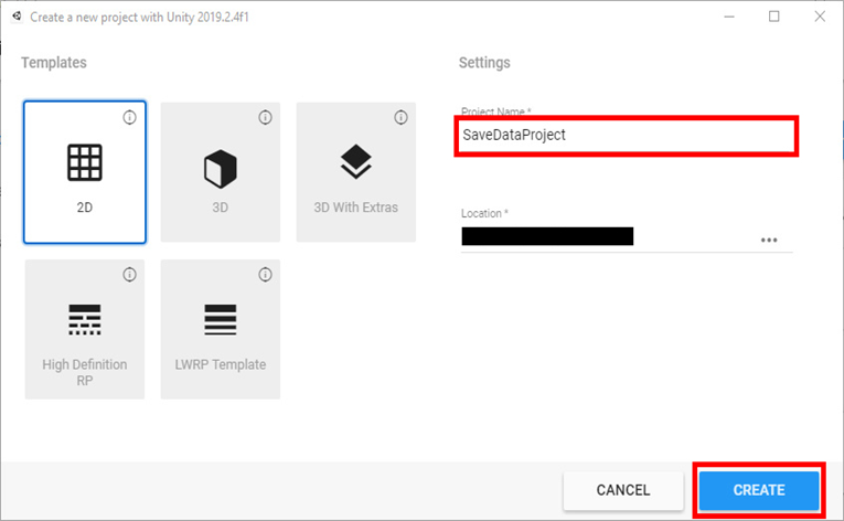
Figure 1: Project creation

Once you create the project, you’ll need two scripts. You create scripts by right-clicking in the Assets window and selecting Create->C# Script as shown in Figure 2. Call these scripts SavePrefs and SaveSerial.
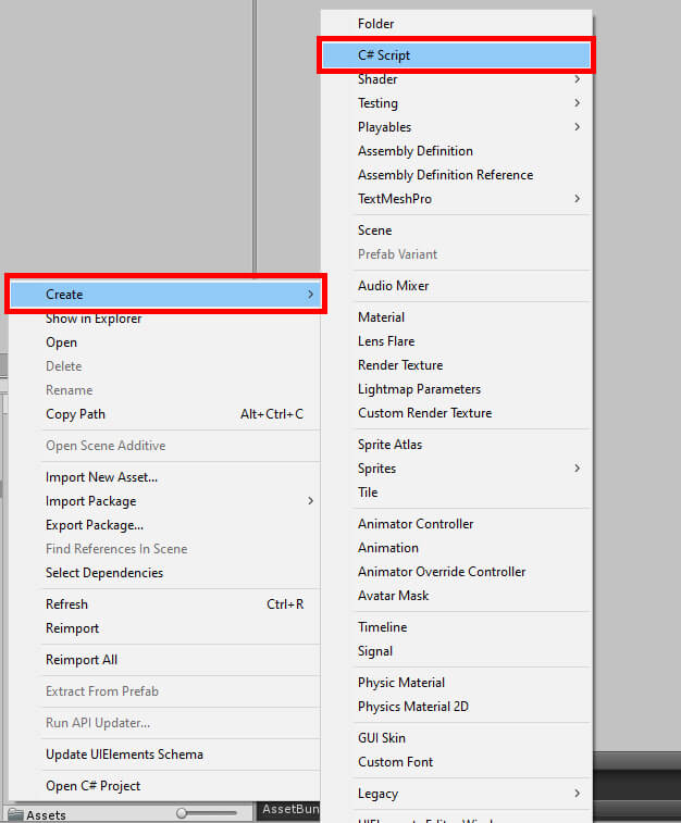
Figure 2: Script creation

To see what saving a game entails, start with the SavePrefs script. Double-click the script to open Visual Studio.

PlayerPrefs – The Easy Way

To begin, the Start and Update methods can be commented out or deleted as they will not be used to demonstrate the save functionality. Next, some variables to hold the values to save will be needed.

int intToSave;
float floatToSave;
string stringToSave = "";

Next, the OnGui method will create a Graphical User Interface (GUI) from code to manipulate these values. Two buttons created in the method will increase intToSave and floatToSave, and a text field will be made for stringToSave. The code will also create a few labels made to show the current values of these variables. Finally, three more buttons will be made that save, load, and reset data.

void OnGUI()
{
        if (GUI.Button(new Rect(0, 0, 125, 50), "Raise Integer"))
                intToSave++;
        if (GUI.Button(new Rect(0, 100, 125, 50), "Raise Float"))
                floatToSave += 0.1f;
        stringToSave = GUI.TextField(new Rect(0, 200, 125, 25), 
               stringToSave, 15);
        GUI.Label(new Rect(375, 0, 125, 50), "Integer value is " 
               + intToSave);
        GUI.Label(new Rect(375, 100, 125, 50), "Float value is " 
               + floatToSave.ToString("F1"));
        GUI.Label(new Rect(375, 200, 125, 50), "String value is " 
              + stringToSave);
        if (GUI.Button(new Rect(750, 0, 125, 50), "Save Your Game"))
                SaveGame();
        if (GUI.Button(new Rect(750, 100, 125, 50), 
                "Load Your Game"))
                LoadGame();
        if (GUI.Button(new Rect(750, 200, 125, 50), 
                "Reset Save Data"))
                ResetData();
}

The last three buttons all call methods whenever they are clicked, but those methods have not been defined yet. This will be fixed now, starting with the SaveGame method.

void SaveGame()
{
        PlayerPrefs.SetInt("SavedInteger", intToSave);
        PlayerPrefs.SetFloat("SavedFloat", floatToSave);
        PlayerPrefs.SetString("SavedString", stringToSave);
        PlayerPrefs.Save();
        Debug.Log("Game data saved!");
}

No, your eyes do not deceive you. The actual act of saving your game takes only a few lines of code. So, what’s happening? Well, as promised, PlayerPrefs saves the player’s game. First, you must set some variables for PlayerPrefs to save. As seen above, three variables were set, all of them given a name, or key, followed by the variable to save. Once PlayerPrefs is given all its information, Save is called and, as you may have guessed, saves the data. A message is also printed to Unity’s debug console as a little note to the developer saying the save was successful.

You may be wondering where this save data is on the computer. On Windows, PlayerPrefs can be found in the Registry under HKEY_CURRENT_USER\Software\Unity\UnityEditor\[company name]\[project name] (Figure 3), where company name and project name are names set up in the project settings. Bear in mind this is the location for when the game was run from the editor. In an exe they can be found at HKEY_CURRENT_USER\Software\[company name]\[project name]. On Mac OS, according to the Unity documentation, the PlayerPrefs is found at ~/Library/Preferences folder, in a file named unity.[company name].[product name].plist.
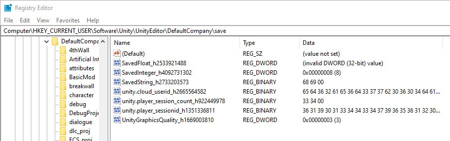
Figure 3: PlayerPrefs variables in the Windows Registry

Loading data is essentially saving data done in reverse. You set your variables of choice to whatever is in PlayerPrefs, and you’re good to go. A good practice is to make sure that the PlayerPrefs for your game has at least one of the keys you’re looking for. In other words, you’re checking that there’s any save data to be found. The code sample below uses HasKey to search for one of the keys declared in the SaveGame method, those keys being SavedInteger, SavedFloat, and SavedString. Looking for just one will be sufficient. So long as PlayerPrefs has one of those, it’s safe to assume it will have the remaining data. Otherwise, it will print an error to the Unity console.

void LoadGame()
{
        if (PlayerPrefs.HasKey("SavedInteger"))
        {
                intToSave = PlayerPrefs.GetInt("SavedInteger");
                floatToSave = PlayerPrefs.GetFloat("SavedFloat");
                stringToSave = PlayerPrefs.GetString("SavedString");
                Debug.Log("Game data loaded!");
        }
        else
                Debug.LogError("There is no save data!");
}

Finally, if you wish to remove the save data stored in PlayerPrefs, all you need to call is PlayerPrefs.DeleteAll and the work is complete. In the following method, DeleteAll is put to use along with resetting the variables and ending by printing a message to the debug console.

void ResetData()
{
        PlayerPrefs.DeleteAll();
        intToSave = 0;
        floatToSave = 0.0f;
        stringToSave = "";
        Debug.Log("Data reset complete");
}

To try it out in-game, save your code and return to the Unity editor. Attach the SavePrefs script to an object, such as Main Camera as shown in Figure 4.
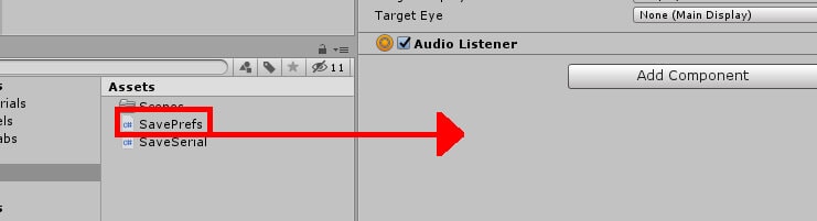
Figure 4: Attaching the SavePrefs script.

Begin playing the game and tinkering with the GUI on-screen, changing variables to whatever you wish. When ready, save your game. Then try stopping and replaying the game, this time clicking the Load Your Game button. Provided everything works correctly, you should see the variables immediately change to whatever was saved to PlayerPrefs. In addition, you can wipe PlayerPrefs clean by clicking the Reset Save Data button. Figure 5 shows the game in action.
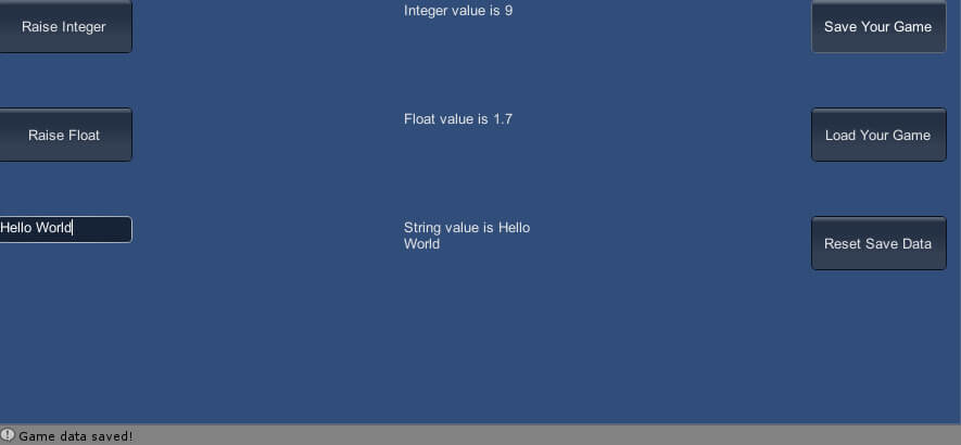
Figure 5: The project in action, using PlayerPrefs

This method seems simple and effective, so why wouldn’t you use PlayerPrefs all the time? Well, PlayerPrefs is one of the least secure ways to save your data, and thus you wouldn’t want to save anything in PlayerPrefs that you absolutely do not want a potential player tampering with. This could be things like how much in-game currency the player currently possesses or stats in a role-playing game. As the name implies, best practices for PlayerPrefs is typically storing a player’s preferences and other trivial data. For example, if you’re letting the user customize the look and size of the game’s UI, PlayerPrefs would be an excellent way to store those preferences.

There’s also the issue of flexibility. The project’s SaveGame method saves an int, float, and string. These are all the data types you can save to PlayerPrefs, so if you wish to save variables of other types, you may be out of luck. Fortunately, there is the “not so easy way” of doing things that allows more flexibility in what you can save, not to mention a little extra security.

Serialization – The Not So Easy Way

Open up the SaveSerial script to begin trying out the next method. Much of the code will be the same as the last script with some minor differences to prove certain points. Here’s the variables and OnGUI method that will be used. All remaining methods will be different.

int intToSave;
float floatToSave;
bool boolToSave;
void OnGUI()
{
        if (GUI.Button(new Rect(0, 0, 125, 50), "Raise Integer"))
                intToSave++;
        if (GUI.Button(new Rect(0, 100, 125, 50), "Raise Float"))
                floatToSave += 0.1f;
        if (GUI.Button(new Rect(0, 200, 125, 50), "Change Bool"))
                boolToSave = boolToSave ? boolToSave 
                       = false : boolToSave = true;
        GUI.Label(new Rect(375, 0, 125, 50), "Integer value is " 
                + intToSave);
        GUI.Label(new Rect(375, 100, 125, 50), "Float value is " 
                + floatToSave.ToString("F1"));
        GUI.Label(new Rect(375, 200, 125, 50), "Bool value is " 
                + boolToSave);
        if (GUI.Button(new Rect(750, 0, 125, 50), "Save Your Game"))
                SaveGame();
        if (GUI.Button(new Rect(750, 100, 125, 50), 
                "Load Your Game"))
                LoadGame();
        if (GUI.Button(new Rect(750, 200, 125, 50), 
                "Reset Save Data"))
                ResetData();
}

To start, a few using statements will be needed to save data using serialization.

using System;
using System.Runtime.Serialization.Formatters.Binary;
using System.IO;

Next, in order to save data, a new class within this script will be created. This class will be made serializable and will consist of the data to be saved.

[Serializable]
class SaveData
{
    public int savedInt;
    public float savedFloat;
    public bool savedBool;
}

I’ve included a screenshot (Figure 6) here to make it easier to understand where this code will go:
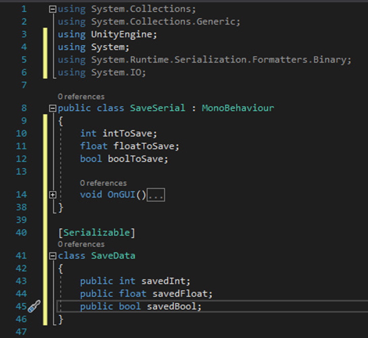
Figure 6: SaveSerial script

The goal now is to create the remaining methods that will allow you to save, load, and reset save data. You might notice that the three variables in the SaveData class correspond with the three variables in SaveSerial. Saving data will work by passing SaveSerial's variable values into SaveData and then serializing the SaveData class itself. Returning to the SaveSerial class, create the following method under the OnGUI method.

void SaveGame()
{
        BinaryFormatter bf = new BinaryFormatter(); 
        FileStream file = File.Create(Application.persistentDataPath 
                 + "/MySaveData.dat"); 
        SaveData data = new SaveData();
        data.savedInt = intToSave;
        data.savedFloat = floatToSave;
        data.savedBool = boolToSave;
        bf.Serialize(file, data);
        file.Close();
        Debug.Log("Game data saved!");
}

The BinaryFormatter is used to perform the act of serialization and deserialization. When serializing the data, BinaryFormatter is responsible for converting the information to a stream of 1s and 0s. FileStream and File are used to create a save file with the dat extension under the application’s “persistent data path” followed by any remaining path you wish to make. The persistent data path is C:\Users\[user]\AppData\LocalLow\[company name].

A new instance of SaveData is created, and the variables within SaveData are given the variables in SaveSerial. The BinaryFormatter serializes that data to the file defined in the FileStream. The file is then closed, and a message is printed to the debug console saying the data was saved. Like before, the LoadGame method is very much the same but in reverse.

void LoadGame()
{
        if (File.Exists(Application.persistentDataPath 
                   + "/MySaveData.dat"))
        {
                BinaryFormatter bf = new BinaryFormatter();
                FileStream file = 
                   File.Open(Application.persistentDataPath 
                   + "/MySaveData.dat", FileMode.Open);
                SaveData data = (SaveData)bf.Deserialize(file);
                file.Close();
                intToSave = data.savedInt;
                floatToSave = data.savedFloat;
                boolToSave = data.savedBool;
                Debug.Log("Game data loaded!");
        }
        else
                Debug.LogError("There is no save data!");
}

Your save file by the name of MySaveData.dat is searched for in the same path given in the SaveGame method. Assuming it’s found, it will open the file and deserialize it using BinaryFormatter. Then the variables found in the save file will be fed into SaveSerial's variables. At the end, a message is printed to the debug console saying the load was performed successfully. If there is no file found at the file path, an error message will display instead.

Finally, there’s the act of deleting and resetting save data. This is extremely similar to the PlayerPrefs method but with a couple of extra steps. Unity will first check to make sure there’s a file at the save location before attempting any deleting of files. Assuming there is a file to delete, the variables in this script will also be reset to some default values and a message printed to the console. Like within the LoadGame method, an error message will be printed to the console if there is no file to be found.

void ResetData()
{
        if (File.Exists(Application.persistentDataPath 
                  + "/MySaveData.dat"))
        {
                File.Delete(Application.persistentDataPath 
                          + "/MySaveData.dat");
                intToSave = 0;
                floatToSave = 0.0f;
                boolToSave = false;
                Debug.Log("Data reset complete!");
        }
        else
                Debug.LogError("No save data to delete.");
}

This concludes this script showcasing saving via serialization. Once again, save the code and go back to Unity. Attach SaveSerial to the same object as before and disable the SavePrefs script component.
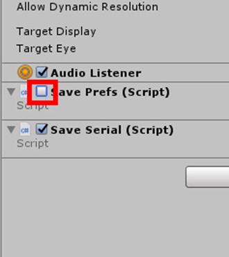
Figure 7: Disabling the Save Prefs component.

When you run the game, the same UI from earlier appears with some alterations. Tinker with the variables like last time and try saving the game. This time a file is saved to the “persistent data path” of the game, which can be found at C:\Users\username\AppData\LocalLow\project name on Windows and ~/Library/Application Support/companyname/productname on Mac, according to the Unity documentation. Close and reopen the game, then click the load button to bring those values back into the game. And of course, you can delete the saved data entirely if you so desire.
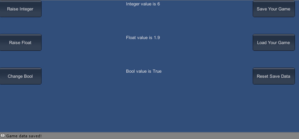
Figure 8: The project in action, using serialization

Conclusion

Barring some very specific exceptions, such as games designed around short play sessions or “perma-death” (perma-death is a game mechanic where once the player loses the game they have to start completely over and everything resets), saving data will be crucial for user retention. Even in those aforementioned examples, most games will at least save a high score or an achievement. What data is saved and how you save that data is down to you and your project’s needs.

Though less secure and limited in what it can save, PlayerPrefs can be helpful for saving a player’s in-game preferences or for games where it doesn’t matter much if the user tinkers with the variables outside the game. In addition, it’s very simple to use which can help save some development time. Meanwhile, serializing data to a file is more complicated but in return, you can save many other types of data and have more security. Like many things in game development, the tools available to you can be utilized in a variety of ways. However, you choose to save your game’s data, there will be options available to you. In the end, the best method is the one that helps you and your project the most.


The post Saving Game Data with Unity appeared first on Simple Talk.


from Simple Talk https://ift.tt/2Ongmmp
via

Saturday, February 1, 2020

Copying of all data between SQL Server databases and servers

This script will copy out all the tables from one version of a database as native BCP format, and  place them in a directory of your choice, (defaulting to your user area in a  directory called BCPFiles). They are placed in sub directories based on your server name and database name, just to keep things neat. It will then if you wish, copy it out to a target server.  On first glance, this routine may seem over-complicated but it is designed to be able to perform this task for a list of these pairs of source & target databases for multi-database  applications if you feel bold. it will allow you to copy the files out just once, and then copy them out to a number of target databases on different servers subsequently. (you determine whether a source or target server is used simply by assigning a $null to $DataSource or $DataTarget when you don’t want the operation to happen).

The script then will transfer this data to an empty version of the same database (same meaning with the same table schema) with no data in it.  If the two versions have a different table structure you’ll get an error. If you use this system and you change the table structure, or constraints, you run your migration code on the source until it is the same as the target.

BCP needs to be installed to run this. This comes with SSMS so you probably have it already. Sometimes you need to create an alias for BCP but I think that problem has gone away

To get started, fill in the connection string for your source of data $datasource and $dataTarget. You also need to fill in an array of objects, each of which define your source and target databases, so you can do a whole list of databases. If you have to use credentials rather than integrated windows security, you add the userID but not the password. You will be asked the first  time you run the routine for your password and this is then stored as an encrypted string in a file in your user area protected by NTFS security. Be warned, though, that you shouldn’t allow anyone else to run this using  your PC, logged in with your credentials. If you don’t want to copy data out of the database into the directory, then set $datasource to $null. Likewise, If you don’t want to copy data in to the target , then set $datatarget to $null. 

This script uses SMO in order to get the list of tables from the database and command-line BCP to do the copying of the data. I’ve published other ways of doing this over the years.

$Filepath = "$env:USERPROFILE\BCPFiles" # local directory to save build-scripts to
$DataSource = @{ 'ConnectionString' = 'Server=MySourceServer;Persist Security Info=False' }; # server name and instance
$DataTarget = @{ 'ConnectionString' = 'Server=MyTargetServer;User Id=sa;Persist Security Info=False' }; # server name and instance

$FileSourceDirectory = 'MyServer'<#if you are reading files in only, the script
needs to know the subdirectory of your root directory to use to get the right files#>

if ($DataSource -eq $null -and $FileSourceDirectory -eq $null)
{ write-error 'the script needs to know the subdirectory of your root directory to use' break; }


$Databases = @(@{ 'source' = 'MyDatabase'; 'target' = 'MyNewDatabase' })
$slash = '+' #the string that you want to replace for the 'slash' in an instance name for files etc

# set "Option Explicit" to catch subtle errors
set-psdebug -strict
$ErrorActionPreference = "stop" # you can opt to stagger on, bleeding, if an error occurs
#load the sqlserver module
$popVerbosity = $VerbosePreference
$VerbosePreference = "Silentlycontinue"
# the import process can be very noisy if you are in verbose mode
Import-Module sqlserver -DisableNameChecking #load the SQLPS functionality
$VerbosePreference = $popVerbosity

if (!(Test-Path -path $Filepath -PathType Container))
{ $null = New-Item -ItemType directory -Path $Filepath }


@($DataSource, $DataTarget) | where { $_ -ne $null } | foreach {
        $csb = New-Object System.Data.Common.DbConnectionStringBuilder
        $csb.set_ConnectionString($_.ConnectionString)
        if ($csb.'user id' -ne '') #then it is using SQL Server Credentials
        { <# Oh dear, we need to get the password, if we don't already know it #>
                $SqlEncryptedPasswordFile = `
                "$env:USERPROFILE\$($csb.'user id')-$($csb.server.Replace('\', $slash)).xml"
                # test to see if we know about the password in a secure string stored in the user area
                if (Test-Path -path $SqlEncryptedPasswordFile -PathType leaf)
                {
                        #has already got this set for this login so fetch it
                        $SqlCredentials = Import-CliXml $SqlEncryptedPasswordFile
                        
                }
                else #then we have to ask the user for it (once only)
                {
                        #hasn't got this set for this login
                        $SqlCredentials = get-credential -Credential $csb.'user id'
                        $SqlCredentials | Export-CliXml -Path $SqlEncryptedPasswordFile
                }
                $_.ServerConnection =
                new-object `
                                   "Microsoft.SqlServer.Management.Common.ServerConnection"`
                ($csb.server, $SqlCredentials.UserName, $SqlCredentials.GetNetworkCredential().password)
                $csb.Add('password', $SqlCredentials.GetNetworkCredential().password)
        }
        else
        {
                $_.ServerConnection =
                new-object `
                                   "Microsoft.SqlServer.Management.Common.ServerConnection" `
                ($csb.server)
        }
        $_.csb = $csb
        try # now we make an SMO connection to the server, using the connection string
        {
                $_.srv = new-object ("Microsoft.SqlServer.Management.Smo.Server") $_.ServerConnection
        }
        catch
        {
                Write-error "Could not connect to SQL Server instance $($DataSource.csb.server) $($error[0]). Script is aborted"
                exit -1
        }
} <# all this work just to maintain passwords ! #>
if ($DataSource -ne $null)
{
        $DirectoryToSaveTo = $DataSource.csb.server.Replace('\', $slash)
        if ($DataSource.srv.Version -eq $null) { Throw "Can't find the instance $($DataSource.csb.server)" }
        Write-verbose "writing data out to $directoryToSaveTo"
        $DataSource.srv.Databases[$Databases.source].Tables | Select Name, Schema |
        foreach{
    <# calculate where it should be saved #>
                $directory = "$($FilePath)\$($DirectoryToSaveTo)\$($Databases.Source)\Data"
    <# check that the directory exists #>
                if (-not (Test-Path -PathType Container $directory))
                {
      <# we create the  directory if it doesn't already exist #>
                        $null = New-Item -ItemType Directory -Force -Path $directory;
                }
                $filename = "$($_.Schema)_$($_.Name)" -replace '[\\\/\:\.]', '-'
                Write-Verbose "Writing out $($_.Schema).$($_.Name) t0 $($directory)\$filename.bcp"
                If ($DataSource.csb.'user id' -eq '')<# OK. Easy, a trusted connection #>
                {
                        #native format -n, Trusted connection -T
                        $Progress = BCP "$($_.Schema).$($_.Name)"  out  "$($directory)\$filename.bcp"   `
                                                        -n -T "-d$($Databases.source)"  "-S$($DataSource.csb.server)"
                }
                else <# if not a trusted connection we need to provide a userid and password #>
                {
                        
                        $Progress = BCP "$($_.Schema).$($_.Name)"  out  "$($directory)\$($_.Schema)_$($_.Name).bcp"  `
                                                        -n "-d$($Databases.source)"  "-S$($DataSource.csb.server)"  `
                                                        "-U$($DataSource.csb.'user id')" "-P$($DataSource.csb.password)"
                }
                
                if (-not ($?) -or $Progress -like '*Error*') # if there was an error
                {
                        throw ("Error with data export of $($directory)\$($_.Schema)_$($_.Name).bcp - $Progress");
                }
        }
}
if ($DataTarget -ne $null)
{
        if ($DataSource -ne $null) { $DirectoryToLoadFrom = $DataSource.csb.server.Replace('\', $slash) }
        else { $DirectoryToLoadFrom = $FileSourceDirectory }
        if ($DataTarget.srv.Version -eq $null) { Throw "Can't find the instance $($DataTarget.csb.server)" }
        If ($DataTarget.srv.Databases[$Databases.target] -eq $null)
        { Throw "Can't find the database $($Databases.target) on instance $($DataTarget.csb.server)" }
        Write-verbose "Reading data in from $DirectoryToLoadFrom"
        
        $DataTarget.srv.Databases[$Databases.target].Tables | Select Name, Schema |
        foreach {
                # calculate where it gotten from #
                $directory = "$($FilePath)\$($DirectoryToLoadFrom)\$($Databases.Source)\Data"
                $filename = "$($_.Schema)_$($_.Name)" -replace '[\\\/\:\.]', '-'
                $progress = '';
                Write-Verbose "Reading in $($_.Schema).$($_.Name) from $($directory)\$filename.bcp"
                if ($DataTarget.csb.'user id' -ne '')
                {
                        $Progress = BCP "$($Databases.target).$($_.Schema).$($_.Name)" in "$($directory)\$filename.bcp" -q -N -E `
                                                        "-U$($DataTarget.csb.'user id')"  "-P$($DataTarget.csb.password)" "-S$($DataTarget.csb.server)"
                }
                else
                {
                        $Progress = BCP "$($Databases.target).$($_.Schema).$($_.Name)" in `
                                                        "$($directory)\$filename.bcp" -q -N -T -E `
                                                        "-S$($DataTarget.csb.server)"
                }
                if (-not ($?) -or $Progress -like '*Error*') # if there was an error
                {
                        throw ("Error with data import  of $($directory)\$($_.Schema)_$($_.Name).bcp - $Progress ");
                }
        }
        try # now we make an SMO connection to the server, using the connection string
        {
                $DataTarget.srv.ConnectionContext.ExecuteNonQuery(" use [$($Databases.target)]   EXEC sp_msforeachtable 'ALTER TABLE ? WITH CHECK CHECK CONSTRAINT all'")
        }
        catch
        {
                Write-error "there was a constraint error!  Script is aborted"
                exit -1
        }
}


The post Copying of all data between SQL Server databases and servers appeared first on Simple Talk.


from Simple Talk https://ift.tt/38UdCES
via

Wednesday, January 22, 2020

Storage 101: The Language of Storage

The series so far:

Storage drives come in many shapes and sizes, and it can be difficult to distinguish one from the other beyond their appearances because vendor-supplied information is sometimes confusing and obscure. Although the material has gotten better over the years, it can still be unclear. Yet understanding this information is essential to knowing how well a drive will perform, how much data it will hold, its expected lifespan, and other important features.

In the first article in this series, I introduced you to a number of storage-related concepts, all of which can play an important role in determining what each drive offers and how they differ. For example, a solid-state drive (SSD) that uses the Peripheral Component Interconnect Express (PCIe) interface will typically perform better than one that uses the Serial Advanced Technology Attachment (SATA) interface, and a SATA-based SSD will likely perform better than a SATA-based hard-disk-drive (HDD).

But the interface and drive type are only part of the equation when it comes to choosing storage media. You must also take into account latencies, input/output operations per second (IOPS), throughput, effective and usable capacities, data transfer size or I/O size, endurance, and other factors. Unfortunately, it’s no small matter trying to make sense of all these variables, especially with the inconsistencies among storage vendors in how they present information about their products.

In this article, I dig into concepts commonly used to describe storage media to help make sense of the information you’ll encounter when evaluating HDDs or SSDs for your organization. Many of the concepts are specific to performance, but I also discuss issues related to capacity and lifespan, particularly in how they differ between HDDs and SSDs.

Making Sense of Performance Metrics

When architecting storage solutions to meet enterprise requirements such as performance, you should identify the workloads that the devices must support. To this end, you must understand data access patterns such as read operations versus writes, random operations versus sequential, and block transfer size.

In this regard, storage operations can be divided into four types: random reads, random writes, sequential reads, and sequential writes. In some cases, these operations can be further divided by the block transfer size (small versus large), which depends on the application. Many workloads use a mix of two or more of these types, although they might favor one over the others. Common data access patterns include:

  • Random read/write, small block: A wide variety of applications such as transactional business applications and associated databases.
  • Sequential write, large block: Loading media, loading data warehouse.
  • Sequential read, large block: Reading media, data warehouse aggregations and reporting.
  • Sequential write, small block: Database log writes.
  • Mixed: Any combination of the above. Note that, when multiple sequential workloads are active concurrently, the workload becomes randomized.

When shopping for storage, you’ll encounter an assortment of metrics that describe how well a drive is expected to perform. Understanding these metrics is essential to ensuring that you’re using the right drives to support your specific workloads.

Latency refers to a drive’s response time, that is, how long it takes for an I/O operation to complete. From an application’s perspective, latency is the time between issuing a request and receiving a response. From a user perspective, latency is the only metric that matters.

Vendors list latency in milliseconds (ms) or microseconds (µs). The lower the number, the shorter the wait times. However, the rate can quickly increase as individual I/O requests start piling up, the I/O sizes increase (which typically range between 4 KB to 512 KB), or the nature of the workload changes, such as changing from read-only to read/write or from sequential to random. For example, a drive’s latency might be listed as 20ms, but if the drive is supporting concurrent read operations, I/O requests could end up in a long queue, causing a dramatic increase in latency.

Latency is nearly always a useful metric when shopping for drives and should be considered in conjunction with IOPS. For example, a storage solution that provides 185 IOPS with an average latency of 5ms might deliver better application performance than a drive that offers 440 IOPS but with 30ms latency. It all depends on the workloads that the drives will need to support.

Another common metric is IOPS, which indicates the maximum number of I/O operations per second that the drive is expected to support. An I/O operation is the transfer of data to or from the drive. The higher the number of supported IOPS, the better the performance—at least according to conventional wisdom. In truth, IOPS tells only part of the story and should be considered along with other important factors, such as latency and I/O size. IOPs is most relevant for random data access patterns (and far less important for sequential workloads).

Another important metric is throughput, which measures the amount of data that can be written to or read from a storage drive within a given timeframe. Some resources may refer instead to data transfer rate or simply transfer rate, sometimes according to drive type. For example, you might see transfer rate used more often with HDDs and throughput associated with SSDs. Like other performance metrics, throughput is dictated by the nature of the workload. Throughput is most relevant for sequential data access patterns (and far less relevant for random workloads).

The distinction between sequential and random is particularly important for HDDs because of how data is stored on the platters, although it can also play a role in SSD performance. In fact, there are other differences between the two drive types that you need to understand when evaluating storage. Discussions of device capacity and endurance also follow.

What Sets HDDs Apart

Data is written to an HDD in blocks that are stored sequentially or scattered randomly across a platter. Enterprise drives contain multiple platters with coordinated actuator arms and read/write heads that move across the platters (a topic I’ll be covering more in-depth later in the series).

Whenever an application tries to access the data, the platter’s actuator arm must move the head to the correct track and the platter must be rotated to the correct sector. The time required to do so is referred to as the seek time. The time it takes for the platter to rotate to the correct sector is referred to as the rotational latency.

The duration of an I/O operation depends on the location of the head and platter prior to the request. When the data blocks are saved sequentially on the disk, an application can read and write data in relatively short order, reducing seek times and rotational latencies to practically nothing. If the blocks are strewn randomly across the platters, every operation requires the actuator to move the head to a different area on the platter, resulting in rotational latency and seek time, and therefore slower performance.

Because of these differences, it is essential to evaluate HDDs in terms of the workloads you plan to support, taking into account such factors as file size, concurrency, and data access patterns (random vs. sequential, read vs. write, big block vs. small block, and mixed). By taking your workloads into account, you’ll have a better sense of how to select the right drives for the workloads demanded by your organization’s applications.

For example, Dell offers a 12-TB SATA drive that supports up to 118 IOPS for random reads and 148 IOPS for random operations that include 70% reads and 30% writes at a given latency. Whereas the same drive offers a throughput of 228 MB/s for sequential read and write operations. From these metrics, you can start getting a sense of whether the drive can meet the needs of your anticipated workloads.

Suppose you’re looking for a storage solution to support a set of read-intensive web applications whose storage access pattern is primarily random reads, as opposed to sequential reads. You would want to compare the Dell drive against other drives to determine which one might offer the best IOPS, with less emphasis placed on the other types of access patterns.

One characteristic driving HDD performance is revolutions per minute (RPM), that is, the number of times the drive’s platters rotates within a minute. The higher the number of RPMs, the faster the data can be accessed, leading to lower latency rates and higher performance. Enterprise-class HDDs typically support 10,000 or 15,000 RPMs, often written as simply 10K or 15K RPMs.

You must also take into account a drive’s available capacity, keeping in mind that you never load an HDD anything close to its physical capacity.

A drive’s anticipated lifespan is indicated by the mean time between failures (MTBF) rating, the number of operating hours expected before failure. For example, Dell offers several 14-TB and 16-TB drives with MTBF ratings of 2,500,000 hours, which comes to over 285 years. Such ratings are common, yet in reality drives fail far more frequently than high MTBF suggests. MTBF is only a small part of the reliability equation. Enterprise solutions demand the identification and elimination of single points of failure and redundancies across components, starting at the drive level.

By looking at the various metrics, you have a foundation to begin comparing drives. Historically, marketing considerations—trying to present their drives in the best light—resulted in presenting performance specs in a way that made comparisons across vendors challenging. Today’s specifications are generally more consistent, at least enough to make reasonable apples-to-apples comparisons. Some vendors also provide insights beyond the basics, for example, providing performance metrics featuring a mix of workloads, such as 70% reads and 30% writes at a given latency.

What Sets SSDs Apart

Consumer and enterprise SSDs are based on NAND flash technologies, a type of nonvolatile memory in which data is stored by programming integrated circuit chips, rather than manipulating magnetic properties, as with an HDD. Also unlike the HDD, the SSD has no moving parts, which makes reading and writing data much faster operations.

If you’re relatively new to enterprise SSDs, the terminology that surrounds these drives can be confusing. Yet the fundamental performance considerations are exactly the same: latency, IOPs, throughput, capacity, and endurance .

As with an HDD, capacity in an SSD refers to the amount of data it can hold. With SSDs, however, vendors often toss around multiple terms related to capacity and do so inconsistently, so it’s not always clear what each one means. For example, some vendors list a drive’s total capacity as raw capacity or just capacity, both of which refer to the same thing—the maximum amount of raw data that the drive can hold.

Not all of the drive’s raw capacity is available for storing data. The drive must be able to accommodate the system overhead required to support various internal SSD operations. For this reason, the amount of available capacity is always less than the amount of raw capacity. Vendors often refer to available capacity as usable capacity.

Conceptually, raw capacity and usable capacity are similar between HDDs and SSDs. For example, when calculating capacities, you should take into account that some of that space must be available for system data, as well as for recovery configurations such as RAID.

Another characteristic that sets the SSD apart is the way in which bits are stored in the flash memory cells. Today’s SSDs can store up to four bits per cell, with talk of five bits in the wings. Vendors often reference the bit-level in the drive’s specifications. For example, a drive that supports three bits per cell is referred to as triple-level cell (TLC) flash, and a drive that supports four bits per cell is referred to as quad-level cell (QLC) flash.

In addition to squeezing more bits into a cell, vendors are also trying to get more cells onto a NAND chip. The more bits the chip can support, the greater the data density.

As with HDDs, SSD endurance refers to the drive’s longevity or lifespan; however, it’s measured differently. SSD drive endurance is based on the number of program/erase cycles (P/E cycles) it will support. NAND cells can tolerate only a limited number of P/E cycles. The higher that number, the greater the endurance. A drive’s endurance is measured by its write operations because read operations have minimal impact on an SSD. Whereas the HDD endurance metric is MTBF, vendors report an SSD’s endurance by providing the number of drive writes per day (DWPD), terabytes written (TBW), or both. The DWPD metric refers to the number of times you can completely overwrite the drive’s capacity each day during its warranted lifespan. The TBW metric indicates the total number of write operations that the drive will support over its lifetime. The DWPD and TBW are quite useful for comparing drives.

As vendors squeeze more bits into each cell and more cells into each chip, SSD vendors incorporate sophisticated technologies to mitigate the challenges of maintaining data integrity concomitant with higher data densities. For example, all SSDs employ wear leveling, over-provisioning, garbage collection, and error correction code (ECC) to extend the drive’s life, all of which I’ll be covering in more detail later in the series.

Moving toward a better understanding of storage

You should use the vendors’ published information only as a starting point for evaluating drives and identifying candidates. Consider additional research such as community reviews, benchmarks, or other resources to give you a realistic understanding of a drive’s capabilities. Your goal is to get as complete a picture as possible before investing in and testing solutions.

In addition, when comparing storage solutions, be sure to take into account the effective capacity, which is the amount of storage available to a drive after applying data-reduction technologies such as deduplication and compression. Such data-reduction strategies make it possible for the drive to store much more data. For example, IBM offers a flash-based storage system that provides 36.9 TB of raw capacity but supports up to 110 TB of effective capacity

Clearly, you need to understand a wide range of concepts to determine what types of storage will best support your workloads. Not only must you choose between HDDs and SSDs, but you must also select from within these categories, while taking into account such factors as latency, IOPs, throughput, densities, and numerous others considerations.

In the articles to follow, I’ll be digging into HDDs and SSDs more deeply so you can better understand their architectures and how they differ in terms of capacity, performance, and endurance. With this foundation, you’ll be better equipped to determine what storage solutions you might need for your organization, based on your applications and workloads.

The post Storage 101: The Language of Storage appeared first on Simple Talk.


from Simple Talk https://ift.tt/2NMYsJh
via

Tuesday, January 21, 2020

Managing SQL Server Docker containers in macOS

In the first part of this article series, you learned the basics of SQL Server containers for macOS, starting with a brief definition of what Docker is, how it works (architecture) and how to install it on macOS. Finally, I gave you a quick example on how to pull a Docker image from Microsoft Container registry to create a SQL Server container using the Docker command line client.

In this second part, you will learn in detail about the Docker command line client. My goal is to help you understand how all these commands can help you to manage your SQL Server container through its life cycle.

Container Life Cycle

You may have heard these words before: Containers are ephemeral. Let me tell you, that phrase is absolutely true. Containers are created one day for a specific task and the next day stopped or even deleted to be rebuilt from a recent version of the image that includes minimal changes in the configuration or functionality of the containerized application. That is why you want to become very familiar with the Docker command line client. The better you learn and understand all the command line client instructions to interact with the Docker daemon, the faster you will start developing, shipping and running containerized applications. In this specific case, we are looking forward to becoming proficient managing SQL Server containers.

The life cycle of a container starts by identifying the base image version you want to use for the containerized application. In the previous article, I explained the meaning of the SQL Server image tag (SQL Server Version – build number – operating system). This is the first thing you want to look for when choosing the image from Microsoft Container Registry repository.

Then, the next step is to create the container using the docker run command (see part 1). The problem comes when you don’t want to keep this container up and running all the time. You need to learn how to stop it, modify it or even delete it.

In summary, the container life cycle is basically performing some or all of the following actions:

  • Stop
  • Start
  • Delete

Take a look at how Docker client can help perform all of these container life cycle actions.

Docker Container Management

At this point you should understand that a Docker image is required to create a container. When working with containers, it is pretty common to end up with multiple local copies of Docker images laying around in the local image repository. Probably, these images are from previous test efforts performed using different versions of the same application. SQL Server is not an exception to this problem; you can have multiple images of SQL Server 2017 from the RTM version to the latest CU.

Listing Images

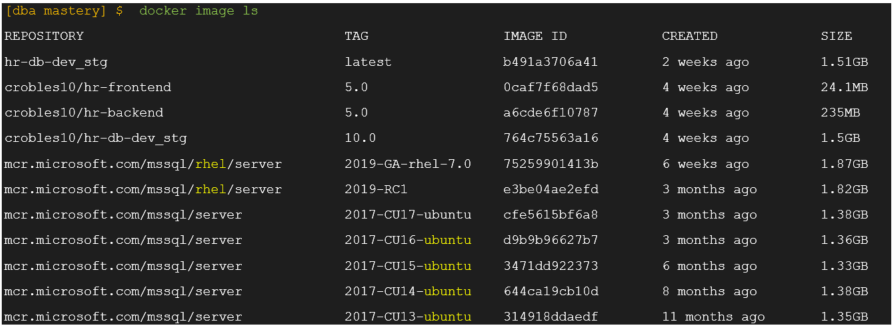
The best way to understand what images are available in the local repository, is using the docker image ls command. This command simply lists all existing images including the repository where it came from, the tag, image ID and its size.

$ docker Image ls

Here is what the output looks like:

As you can see, I have a significant number of images in my local repository, probably because I have been testing several versions of SQL Server 2017 and 2019. If you look closely, you will note I have different images for different operating systems (Ubuntu & RedHat).

Deleting Images

At the time I’m writing this article, SQL Server 2019 is already in GA (General availability), so there is no point for me to keep using the “2019-RC1” (Release candidate) in my local repository. Therefore, for this example I will proceed to remove that image from my local repository.

I need to use the docker image rmi command to help me with this container management action. A requirement for this container management action is to know the docker image ID beforehand, and I already have this information from the previous example:

$ docker image ls

Using the highlighted image ID above, I will proceed to remove the image as follows:

$ docker image rmi e3be04ae2efd

As you can see from the output, the image ID e3be04ae2efd (2019-RC1) was deleted and untagged from my local image repository.

Checking the Container Status

The Docker client provides many ways to check the status of a container. You can easily find the current state of a container and understand what is going on from within the container by checking the logs or simply learn about its CPU and memory utilization.

Now it’s time to put all these theories in practice using the Docker client commands.

docker ps

The docker ps command is a great way to find the current state of all your containers; however, you need to understand how to make the most of it. For example, if this command is executed without any options, it only shows running containers by default.

$ docker ps

The output provides the following information:

  • Container ID
  • Image
  • Command (Last command executed when this container started)
  • Creation date
  • Status
  • Ports
  • Container name

This is a good starting point; however, what happens if you want to learn more about all the other containers that are not actually running? Or filter by name or status? Don’t worry, the docker ps command provides that information and many options more.

Speaking about options, I will focus just in two:

Option name

Command

All

docker ps -a

Filter

docker ps -f

There are many more options of course; however, the two options listed above are the most useful for finding the status of the container quickly and easy.

All (docker ps -a)

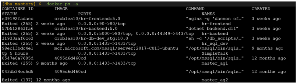
This command requires to combine the docker ps command with the -a option. It will list all containers regardless of their states (running | paused | stopped). This is better than just running the docker ps command without any options, so take a look at the output:

$ docker ps -a

As you can see, the command returns too much information. You may be asking yourself if there is a way to see this output cleaner or make it readable for everybody.



Many Docker client commands have an additional argument called --format just for this purpose. The format must be specified using the “Go” language which is translated to a JSON object to produce the desired output.

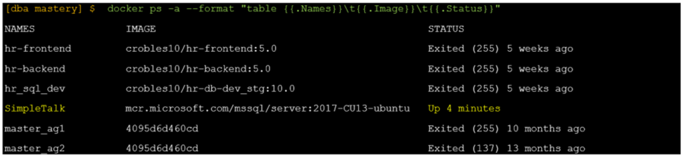
Imagine you want to know more about all your containers, but you are interested to see a customized output including just the container name, the image and the last known status. Here is an example based on this need, where the output will be displayed as a tabbed table displaying just the columns included in JSON format:

docker ps -a --format "table \t\t"

095d6d460cd Exited (255) 9 months ago

master_ag2 4095d6d460cd (137) 12 months ago

This customized output looks way better than the default one, the three columns , and are tab (\t) separated making the text clean and easy to read.

Of course, this is just an example. You are free to customize this output the way you like as this is at least a good starting point.

Filter (docker ps -f)

The filter option is just like a WHERE clause for a query; it will look up a key value to be paired with one of the supported filters:

Filter

Description

id

Container’s ID

name

Container’s name

label

An arbitrary string representing either a key or a key-value pair

status

One of created, restarting, running, removing, paused, exited, or dead

In simple terms, it allows you to search for all those containers with certain ID, name, label or even status.

Here are a few examples of the use of the filter option for different scenarios.

Filtering by Name

Imagine you want to list all those containers that start with the word “Simple.” We add the filter key name to the docker ps -f command assigning the lookup value. Let’s see how it works:

$ docker ps -f "name=Simple"

The output returned is just what I expected. I can see a container with name “SimpleTalk” is listed, which by the way is in “running” status. Note that I didn’t have to specify the exact name; it just found a name that matches with the specified pattern.

Filtering by Name Regardless of the Status

The previous example works well; however, there is a problem with this filter. The results are being limited by the docker ps command because it will list only active (running) containers. In case you want to make sure all containers are listed regardless of the status, you must add the “-a” option to the previous example. This is how it works:

$ docker ps -a -f "name=master"

Note that all the containers with the name “master” are listed. This is good but not quite perfect yet. What about combining everything learned so far? I mean, listing all containers regardless of the state filtered by name and limiting the output to show just the container name, image, port number and status in a tabbed table form.

Here is the command:

$ docker ps -a  -f “name=master” --format "table \t\t"

The output looks good now, clean and easy to read. Importantly, it lists all containers with the word “master” in the name, regardless of its status.

Stopping the Container

The docker stop command is what you want to use to stop one or more containers; you just need to specify the container name. This is very similar to the previous example; however, there is something else that you need to understand, especially when stopping a SQL Server container.

There are multiple termination signals in Linux, used for slightly different purposes. Docker containers uses the SIGTERM and SIGKILL termination signals, but what they are?

SIGTERM

This is a generic signal to terminate a program, it is the traditional way to ask a program to terminate its process.

SIGKILL

This signal causes the immediate termination of a program. This signal cannot be blocked or ignored; it simply kills the program.

Putting all this together means: When the docker stop command is issued, the main process of the container in question–in this case SQL Server–will receive a SIGTERM, giving the program enough time to gracefully shutdown. After this grace period finishes (10 seconds by default), the container will receive a SIGKILL to immediately terminate SQL Server.

Run this command to stop the container:

$ docker stop SimpleTalk

How cool is that! Using just a single line of code you can stop a SQL Server instance. You don’t need to worry about stopping the services anymore when using containers because everything is handled by Docker using the SIGTERM and SIGKILL signals as explained before.

Starting the Container

Booting up a VM or waiting for all the SQL Server services to be started is something from the past. Trust me, containers really change the way to ship and develop applications because of its simplicity. If you are one of those people that likes to get things done quickly and efficiently, you are going to love the container technology.
Starting up a container, requires running the docker start command followed by the name of the container. That’s so simple, right? Take a look at how it works in practice:

$ docker start SimpleTalk

The command returns the name of the container as an indicator that the container called “SimpleTalk” was successfully started.

Deleting the Container

This is the last step in container management, and the obvious step when you are done with the life cycle of your container. The docker rm command has a few options It can remove a container regardless of its status (stopped | running), and it can also remove all containers including its volume.

I will focus on the traditional way, removing a container regardless of its status. Combining the docker rm with the --force option will send a SIGKILL then the container will be immediately removed.

First, check the status of the “SimpleTalk” container:

$ docker ps -a --format "table \t\t"

As you can from the output above, this container has been up and running for the last 4 minutes. Now delete it using the docker rm --force command:

$ docker rm --force SimpleTalk

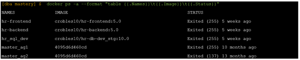
The command returned just the name of the removed container. To make sure it happened correctly, check the status of all the containers again:

The “SimpleTalk” container is gone from the list, which means this container was successfully removed.

Conclusion

Understanding the container life cycle is important, it really helps you to understand better what exactly you are doing when interacting with the Docker daemon through the Docker client commands.

At this point, you should be able to perform all the following actions using Docker for macOS:

  • Pull an image
  • Create a container
  • Check the status of a container
  • Stop, start and delete a container

Please join me in the next article series, where I will focus on examining the Docker container to learn more about its metadata and to connect using a database productivity tool like SQLCMD or Azure Data Studio for macOS.


The post Managing SQL Server Docker containers in macOS appeared first on Simple Talk.


from Simple Talk https://ift.tt/2Gd49fD
via

How to Create an Ubuntu PowerShell Development Environment – Part 1

Microsoft has made great effort over the last few years toward multi-platform compatibility. A large part of the IT world runs on Linux. Microsoft recognizes this and has been deploying a lot of their software to now run on the Linux platform. Visual Studio Code, PowerShell, even SQL Server can now run on Linux. As such, it can be beneficial to create your own Linux development environment on your desktop, whether for doing work or just for learning.

While it would be nice to have a computer to install Linux and our other tools directly on, often referred to as a “bare metal” install, most people don’t have extra computers laying around. The solution to this is the use of a virtual machine. In this article, part 1 of 2, I’ll show you how to setup a virtual machine, often referred to as a VM.

Into that VM, you’ll install a Linux distribution, often referred to as a “distro” in the Linux community. It’s important to understand that Linux is the core of the operating system, often called the kernel. Around this kernel people have developed many server and desktop environments. This article will demonstrate use of the most popular ones, Ubuntu, specifically the 19.10 version.

Part 2 of this series will demonstrate how to install PowerShell, Visual Studio Code, and other tools into the Ubuntu VM.

This will create a foundation for a future article, in which you’ll see how to install Docker, then SQL Server into the VM. You’ll then see how to use PowerShell to work with SQL Server as it runs in the Docker container.

VirtualBox

The first thing you need is virtualization software, this is the software that will host and run the virtual machine. Hyper-V is one choice, and if you have it and are comfortable with it, you are welcome to use it for this project.

Hyper-V does require you to have Windows 10 Pro. Many people, especially those at home, may not have the Pro version. For this article then I will be using VirtualBox.

VirtualBox is free, and easy to use. It is also multi-platform, it will run on Windows, Linux, macOS, and Solaris. This article will cover running it on Windows. Do be aware you cannot run VirtualBox and Hyper-V on the same machine, as they both need exclusive access to the same system resources.

You can obtain VirtualBox by going to their website, https://www.virtualbox.org/ and downloading it. Installation is extremely simple, there are almost no options. You can take the defaults for an easy install.

Ubuntu 19.10

After getting VirtualBox installed, you will need a copy of the Ubuntu 19.10 ISO image. The ISO is a file that can be used to install operating systems. ISOs can be written to a USB key or DVD and used to boot a computer, or in this case as a source for VirtualBox.

Getting the ISO is easy, just go to https://ubuntu.com/ . On the front page in the title bar is a Download link. Clicking on it will take you to the downloads page for 19.10, where you will want to download the desktop version of Ubuntu.

From the downloads, simply save the ISO file to your hard drive. Note if you want to experiment with other versions of Ubuntu, simply go to the Downloads link in the upper right and you’ll find other versions you can experiment with.

Creating the Ubuntu Virtual Machine

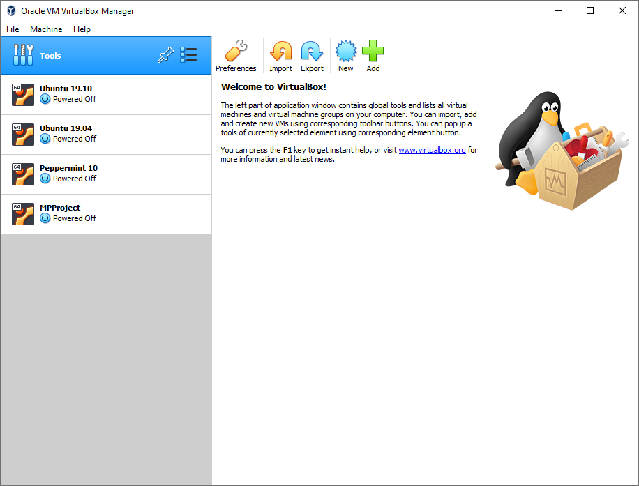
Now you’re ready to take the first step and create the virtual machine. Open VirtualBox, and you’ll see the following screen. In this shot, on the left you will note a list of VMs that I have from other projects, your area will be empty initially but will soon be populated with your own virtual machines.

Setting the VM Name and Type

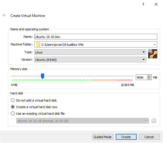
Start by clicking the big New button in the toolbar to begin the process of creating our VM. When you do, the following dialog in appears. Click Expert Mode to see all the options instead of a wizard.

Here you can see I’ve filled out the basic information needed to create the VM. First, I gave it a good name. I took the default for the Machine Folder, that is the path where the virtual machine information will be stored. Note this is for the VM metadata but does not include the location of the virtual hard drive, which will be set in a moment.

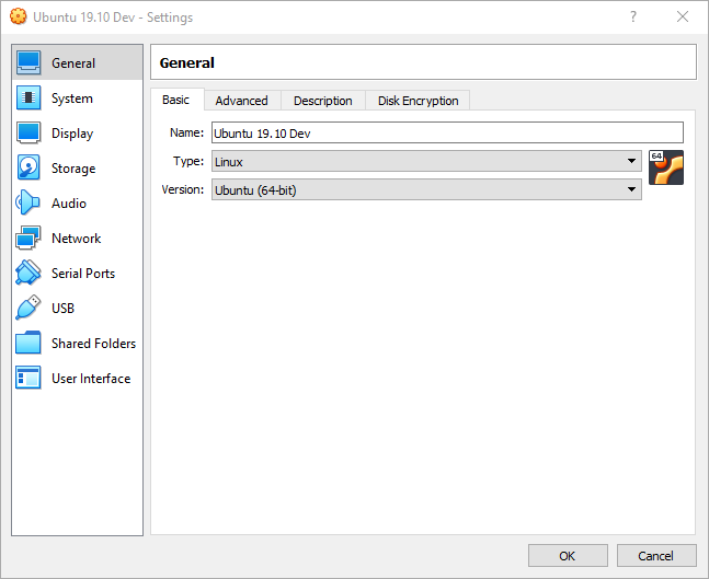
I’ve made sure to set the Type to Linux, and the version to Ubuntu (64 bit). The next setting, Memory size, will be somewhat dependent on the computer you are using. Typically for this type of application you want at least 4 gigabytes, or 4096 megabytes, which is what I have set here.

Finally, make sure the Create a virtual hard disk now is selected the click the Create button.

VM Hard Disk Options

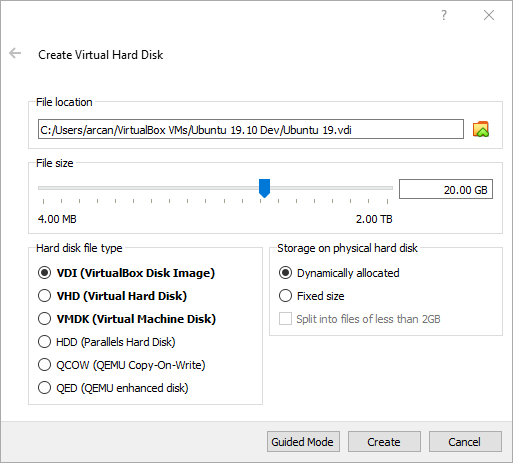
On the next screen you are presented with options about the virtual hard drive that will be created. Here is the screen all filled out.

You can store the virtual hard drive in a different location than the rest of the VM’s data. The File location box is used to indicate that location. A helpful hint, often you can get a performance boost by storing your virtual hard drives on a different physical hard drive than the one of the host operating system. Commonly, the operating system running on the computer itself is referred to as the host operating system. Any virtual machines are known as the guest operating system.

Next up is the File size. Because you will be working with SQL Server, you may need extra space, so initially I recommend setting this to 20 GB. You can do so by using the slider bar, or simply typing into the box to the left of the slider.

On the lower left is the file type, and there are multiple choices. VDI is the native type for VirtualBox, and what will be used for this article. However, VirtualBox also supports types may other types from other virtualization software. VHD is the format for Hyper-V, VMDK for VMWare, and so on. Typically, you would not create a full OS drive in another file type, however this capability may be used later to attach files from other virtualization software to read their data.

Finally, on the lower right, you’ll see the Storage on physical hard disk options. With the Dynamically allocated option, VirtualBox will only take as much space as it needs for the drive, up to the maximum indicated in the file size area (in this case, 20 GB). The second option, Fixed size, will create the virtual disk at its maximum size of 20 GB. Fixed size can perform a bit better as it does not need to worry about checking for disk size and expanding on the fly, it also takes up disk space that may not be needed much of the time. For this article go with the dynamic option and click Create.

Setting Additional VM Options

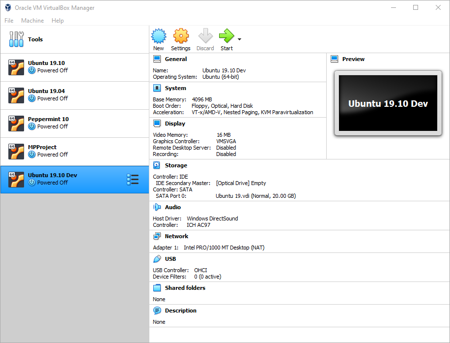
When you create the VM, it now appears in the list on the left. On the right are the machine options.

General Settings

Before you can launch your new VM, there are some settings you need to update. Do note though, if you go into the settings of a running VM many options will be disabled, and this holds true regardless of what virtualization software you are using. You can change the majority of settings only when the VM is shutdown. You won’t have that issue quite yet as you haven’t installed Ubuntu in the VM yet, but it’s something to be aware of for your future use.

Start by clicking on the gold Settings gear icon in the toolbar. As you can see, the dialog that appears allows you to change many options.

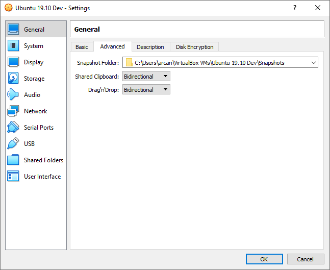
While still on the General settings page, click on the Advanced tab.

On this tab, change the Shared Clipboard and Drag’n’Drop to Bidirectional, as you see above. This will allow you to cut and paste to and from the virtual machine. Likewise, you can copy files into the VM using drag and drop. This is entirely optional, of course, but will make it much easier to work with the VM. Do note that if you are doing security testing of some type, you will wish to alter these settings to either Disabled, or just allow pasting into the VM by picking Host to Guest. However, this is a simple development box so having bidirectional copy/paste will be fine.

System Settings

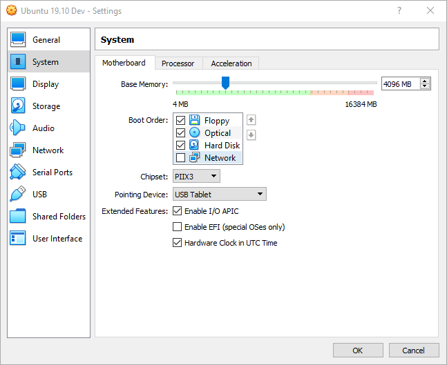
Next, click on the System page on the left to bring up the system settings.

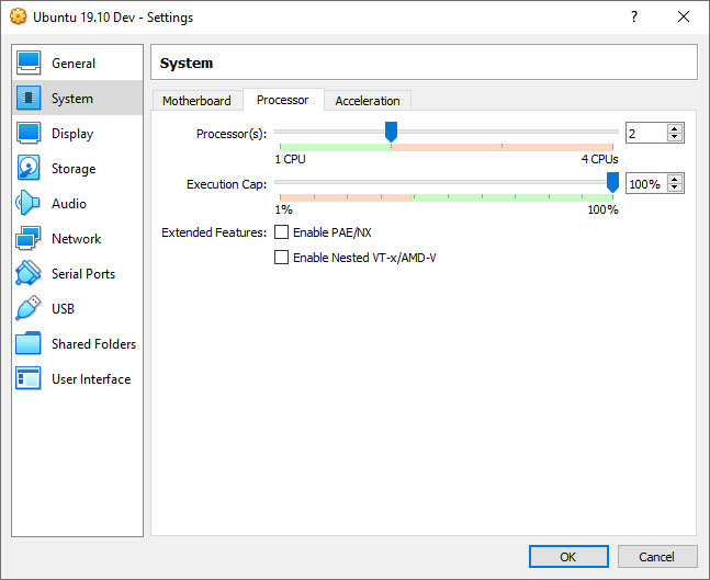
The first tab is the Motherboard; it is on this page where you can change the amount of ram for example. Don’t change anything on this tab, but it very useful to know where to come should you later decide you need to change the amount of ram or any of the other motherboard settings. Take a look at the Processor tab next.

By default, VirtualBox set up this VM with 1 CPU. The computer I’m writing this on has 4 CPUs, so I have opted to increase the CPU count to 2, as you see in the above image. Ultimately this is something you’ll have to determine based on the physical characteristics of your host computer, as well as the demands you’ll be placing on the VM. In my case, I only plan to run one VM at a time, and I won’t be using many resources in the host computer while I am working in the virtual machine.

Now it’s time to move on; click on the Display option on the left.

Display Settings

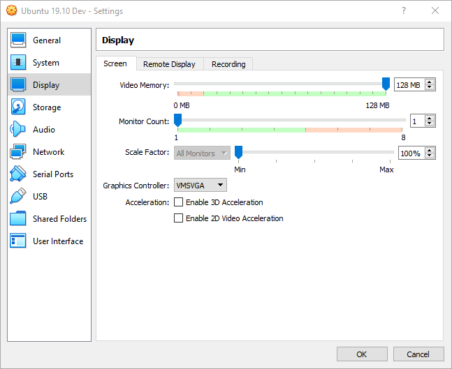
There are a few changes on the Screen tab you should make here to increase performance.

First is the Video Memory. By default, it is at 16MB. I suggest maxing it out to the full 128MB. If you discover later this provides too negative of an impact to your system you can always adjust it to a lower value.

I want to call your attention to the next item, Monitor Count. VirtualBox will let you create multiple virtual monitors, a very helpful utility when you have multiple physical monitors on your host computer. When I first setup a new virtual machine, I always leave this to 1, as you see here. Once I have the VM up and running, I can return here later and add monitors if needed. For example, at home with my laptop hooked to its docking station, I will open the settings and adjust this to 3. Later, when I take my laptop out of the house, I will adjust this back down to 1.

Scaling Factor works just like it does in Windows, it will magnify certain graphical elements in the guest operating system while leaving the resolution alone. I typically leave this set to the default.

The last item of note is the Graphics Controller. We suggest you set to VMSVGA. This setting should allow you to resize the window of your VM, and the VM will then adjust its resolution to fit that of the resized window. However, not all graphics cards respond the same, so you may need to return later and try some of the other settings. Once a virtual machine is created, you can easily go back later and edit things like the graphics controller.

Also be aware some guest operating systems may not support this feature, although the Ubuntu 19.10 used in this article does.

There is one last thing to update, and it is the most important to getting our VM up and running. Click on the Storage icon on the left.

Storage Settings

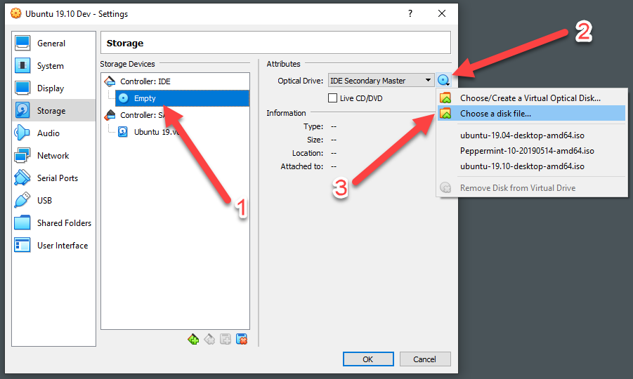
In order to install the Ubuntu, you need to insert the Ubuntu ISO image into the VM’s virtual CD/DVD drive. It is in this step you will accomplish this.

Start by clicking on the Empty label, pointed to by number 1 in the above image.

To the right of the Optical Drive is an icon of a DVD (pointed at by number 2). Click on it to expand the menu.

Now click on Choose a disk file…, indicated by number 3 in the above graphic. Note that if you have installed other VMs in the past, the most recent three ISOs used will appear in the menu. If one of these is the operating system you want to install, you can simply pick it. In this case, navigate to the ISO you downloaded from the Ubuntu site.

Other Settings

There are no more modifications to make in order to proceed. You are free of course to explore the other setting pages. I do want to call your attention to the Shared Folders page. With Shared Folders, you designate a folder location in your host operating system. That folder will then appear inside the file manager inside your guest operating system. This makes it very easy to copy files in and out of your virtual machine.

Just click the big OK button to save your configuration settings and proceed to the next step.

Installing Ubuntu 19.04

Now that you have the machine configured it’s time to get started installing Ubuntu. Make sure the new Ubuntu 19.10 Dev VM is selected in the list of VMs on the left, then click the green Start arrow in the toolbar above the VM settings.

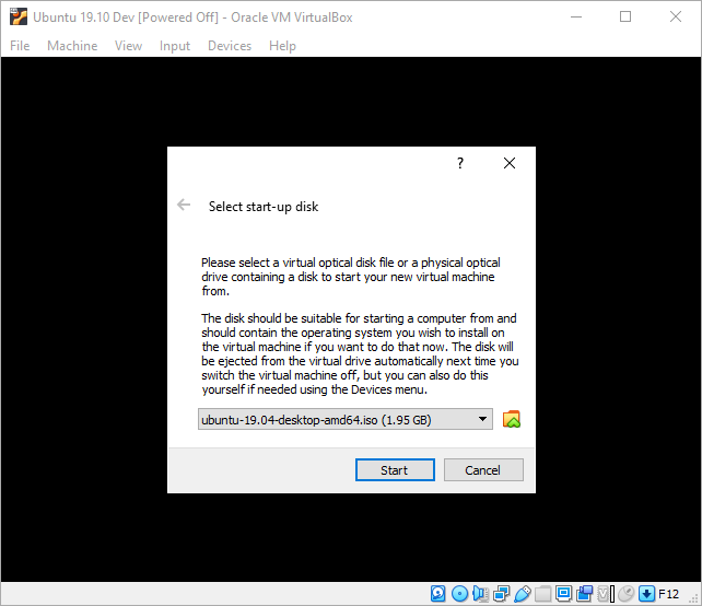
If you forgot to attach the ISO in the previous step, when the machine launches, VirtualBox detects there is no operating system installed. Here it is prompting you for the ISO image to use.

If you remembered to connect it, you’ll skip the above screen. It’s a common mistake to miss attaching the ISO so we wanted to make sure to mention it.

Because you had loaded the Ubuntu ISO in the Storage settings in the previous section, it defaults to it. Just click Start to run the machine with this ISO.

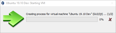
If you are running on a slower machine, you may see the following dialog.

At this point VirtualBox has begun the processes of setting up the VM. Just sit back and wait. The amount of time it will take depends on your computer, so be patient. If you computer is fast enough, you may not see the above dialog box at all.

You will soon see a new window open, with the Ubuntu Virtual Machine. It will take it a little time to spin up, don’t be surprised if you see a blank screen for a little bit. Eventually you will see the Ubuntu installer appear.

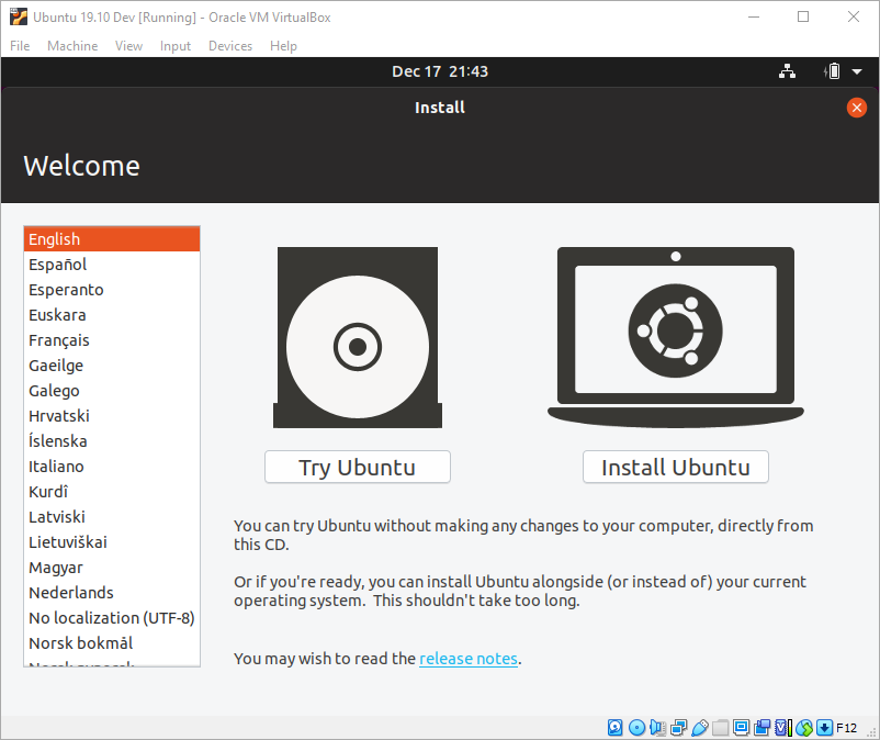
Here you have two choices, Try Ubuntu or Install Ubutnu. Ubuntu is distributed as a Live DVD. In Live mode, you could use a tool to create a bootable USB stick, then boot your physical computer to the USB stick instead of your hard drive. Using the Try option would let you experiment with Ubuntu without making changes to your computer. (If you decide you want to try this for yourself, I recommend the balenaEtcher tool, available at https://www.balena.io/etcher/ ).

In this case you are installing in a virtual machine, with no risk to the host operating system, so after verifying the correct language is selected on the left, click the Install Ubuntu option.

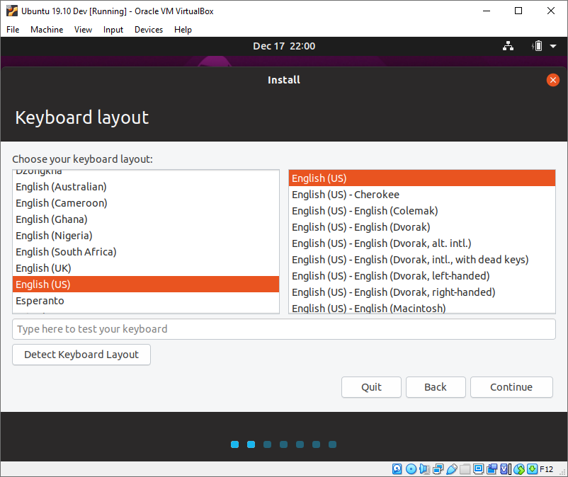
The first thing you are asked is to confirm your keyboard layout. Ubuntu does a good job of figuring it out and picking it automatically, but if you would like to pick something different this is the time to change it. If you are happy, then just click the Continue button.

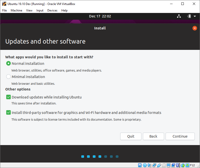
In the next screen, you are given some options. First, it wants to know if you want a normal install or minimal. With minimal, only the web browser and a few basic tools are installed. In normal mode, it will also install office software, media players, and more. I suggest using the Normal Installation option, as it’s often useful to have some of the office tools in your VM. Don’t worry though, if you go with a minimal install, you can easily install other things from the Ubuntu software store that is built into the Ubuntu operating system.

Under the other options, the Download updates… is checked on by default. While you can install updates after installation, it makes it easy to just go ahead and download them now. It will add a bit of time to the setup operation, but if you have a decent internet connection this will be minimal.

The last option, Install third-party software… is unchecked by default. Some Linux users are “purists” and will only use open source software. Others are more pragmatic and are willing to use software that may be closed source or proprietary, such as video and other hardware drivers. I personally fall into the “pragmatic” camp and check this on, as I’ve done here. This is a choice you will have to make, but for this article I suggest checking it on as shown in the above image and click Continue.

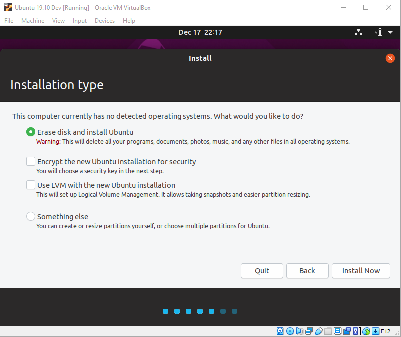
In the next step, you are asked about the installation type. Since the virtual disk is empty, go with the default option of Erase disk and install Ubuntu. The other options are geared toward installation on a physical computer, or into a machine that you want to install Ubuntu side by side with another operating system.

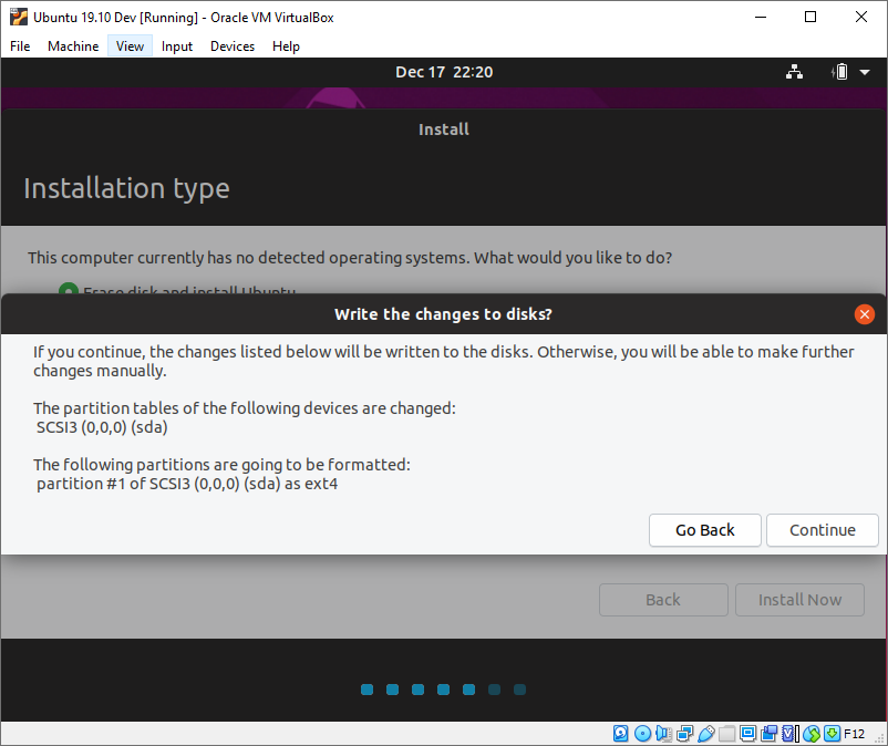
At this point you are ready to begin the installation, so simply click the Install Now button. Because you picked the erase disk option, you are given a warning that you are about to create changes to the target drive.

This is OK, it’s what you want, so just click the Continue button.

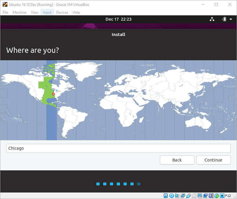
Next, you are asked what time zone you are in. VirtualBox will provide the current date/time info from the host operating system to Ubuntu, and it will default to that time zone. If you need to use another time zone though, this is a good time to change it.

In my case, I am in the Chicago (Central US) time zone, so I will just click Continue.

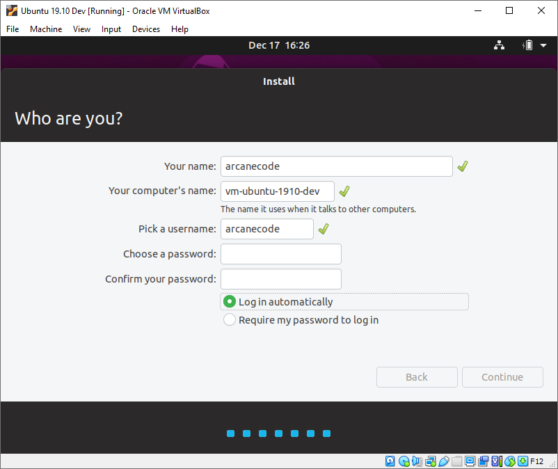
In this next screen, you are asked for some information about your user ID in this virtual machine. Your name is up to you. Typically, you might enter your full name, such as Robert Cain. When it comes to VMs though, I generally use the same information here as my username. For the computer name, I usually begin my virtual machines with vm- in case I am using a network tool. It will be clear this is one of my virtual machines and not a physical computer. After this I’ve added the same information as the name it was given in VirtualBox.

Next up is the username, this is a choice for you to make. Below it you will enter the password to use. Be aware this password is used for more than just logging in. Whenever you install software or alter other system settings, Ubuntu will prompt you for this password as a security measure, to confirm you have permission to make these changes. As a result, you should select a password that is complex enough to be secure, but easy to type and remember as you will be entering it a lot. Note in the above image I haven’t entered the password, when you do it will appear as dots. After entering a password you’ll need to re-enter it in the confirmation box.

The last option is in regard to logging in. The default will be Require my password to login. If you are installing Ubuntu on a physical computer, or in a user testing / production situation, then I highly advise taking this option. In this case, you are creating a machine for simple development and learning so you might want to change it Log in automatically. If this makes you uncomfortable or violates a corporate policy, then by all means go with the default.

Once you are ready, click Continue.

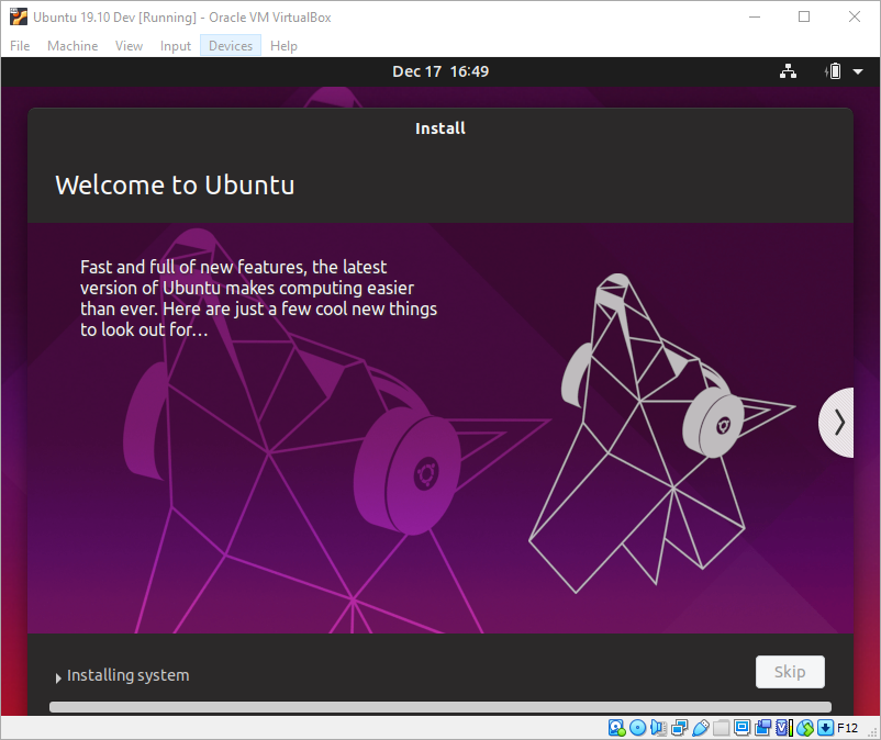
At this point Ubuntu begins installing.

Here you see the progress bar. As it proceeds you will see the display update with helpful tips and tricks. Take a look at them as the install proceeds, it includes some helpful information.

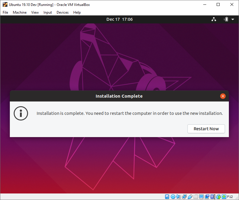
When the installation completes, you will be prompted to restart. Simply click the Restart Now button.

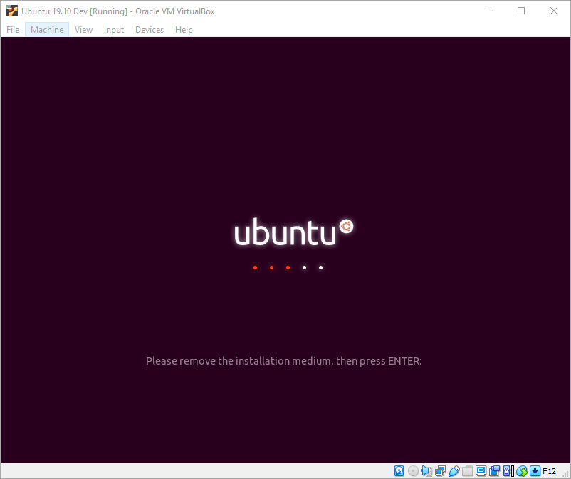
After it reboots, you will be prompted to remove the installation medium then press Enter.

In this case VirtualBox has already taken care of this for you, so all you have to do is click the mouse inside the VM window (so it gets the focus) and press the Enter key.

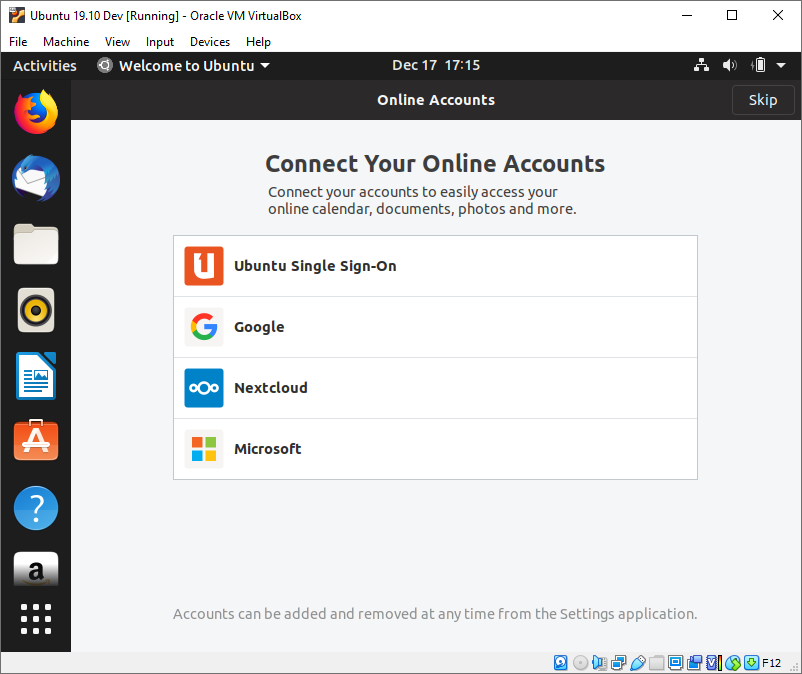
Once Ubuntu restarts again, you will be prompted to connect your online accounts.

Since this is a virtual machine for doing development, I usually skip this step by clicking the Skip button in the upper right.

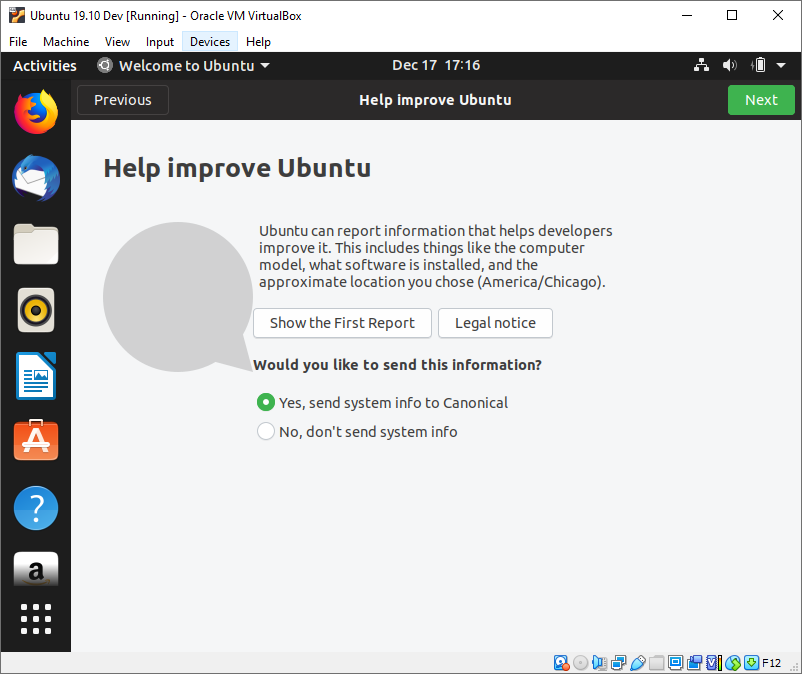
In the next step you are prompted to send system reports to Canonical, the makers of Ubuntu. I usually leave this at the default, but some companies have policies that state you should not share this information. Other people are not comfortable with sharing, so take which ever option you wish and click the Next button in the upper right.

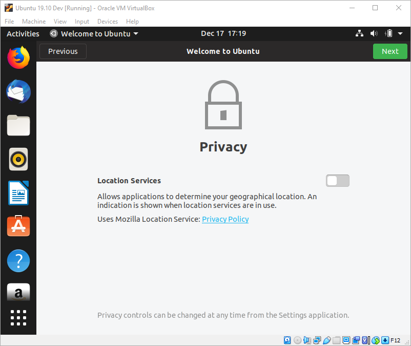
Next Ubuntu wants to know if it can activate Location services. These services are used for things like mapping websites, or when you go to an online store. By default, it is off, and as this isn’t overly useful in a virtual machine (unless you are developing software that needs these services) just take the default and click Next.

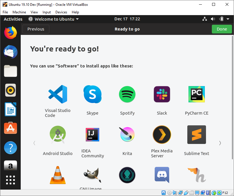
Finally, you’re done! You’ve installed and configured your Ubuntu VM. You can now click Done to close out the window and begin the next steps, updating Ubuntu and installing the software you’ll need.

Updating Ubuntu

In the next article, I’ll go through the process of installing PowerShell, Visual Studio Code (also known as VSCode), and Azure Data Studio. Before that, there are some updates as well as install a few small utilities that will make life easier. You may not use all of them in the next few articles, but as you move forward with your Linux experience, they will become handy to have.

The first thing you’ll find is Ubuntu has a very low timeout before it goes into lock screen mode. In my opinion, when running as a virtual machine, this is unnecessary. Your host system should be set to lock automatically after a set time, or when you choose to lock it manually. Having your virtual machine auto lock as well can get annoying. This first step is optional, but I think you’ll find the short timeout annoying as well, so here’s how to disable it, or if you prefer to extend the time before the VM auto locks.

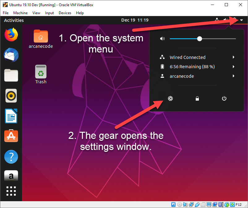
In the upper right corner, next to the battery icon, is a drop-down arrow. Clicking it will bring up a menu.

In the menu, click on the gear icon to bring up the settings window. If you are new to Ubuntu, I’ll mention a few other things. The lock icon in the middle will lock your virtual machine. Getting your machine out of the lock state is a bit odd in that you have to press a key on the keyboard to bring up the password entry dialog. Mouse clicking has no effect.

Next to the lock is the power button, which will give you options to shut down, reboot, and so on.

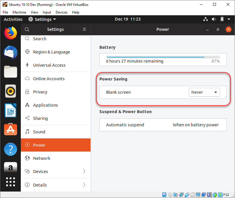
Go ahead and click on the gear. The settings window will now appear. On the left side is a list of settings categories. Scroll down and click on the Power settings.

In the middle is the Power Saving area (highlighted by the orange rectangle in the above graphic). Use the drop-down to change the setting to Never, or to another setting you are comfortable with. There’s no need to press any kind of a save button; when you make a change Ubuntu automatically applies it. Just click the orange X in the upper right corner to close this window.

Opening the Terminal

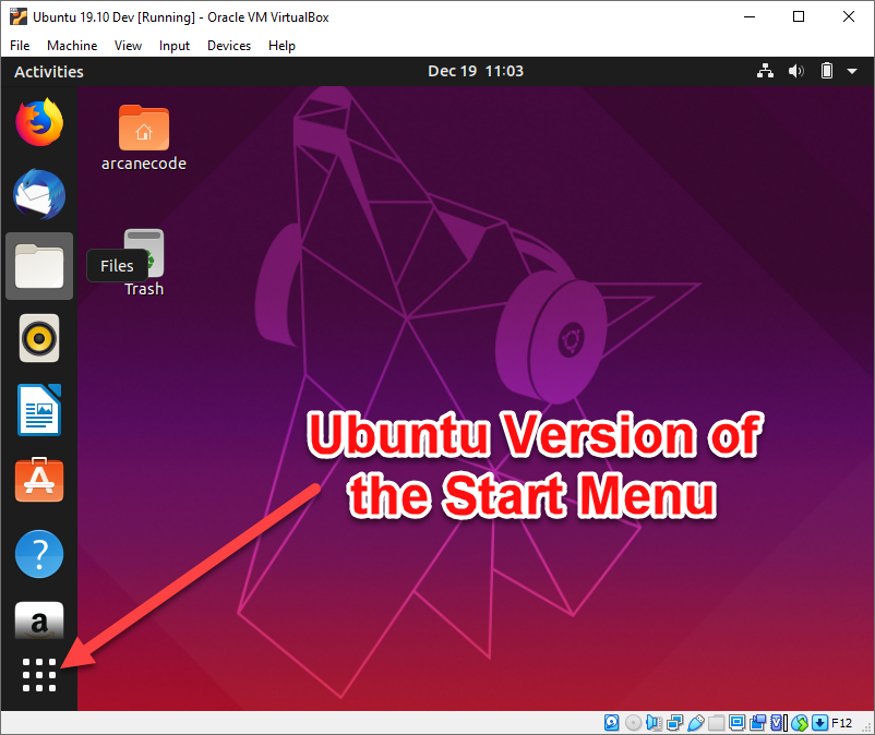
Now that you VM won’t time out on you, you’ll do a general update to Ubuntu itself. You’ll be doing a lot of this through the terminal, so go ahead and open a terminal window. The 9 dot grid in the bottom left of the Ubuntu desktop is similar to the start menu in Windows. Click on it to bring up your installed applications.

After clicking on the “start menu” the screen updates to show all your apps.

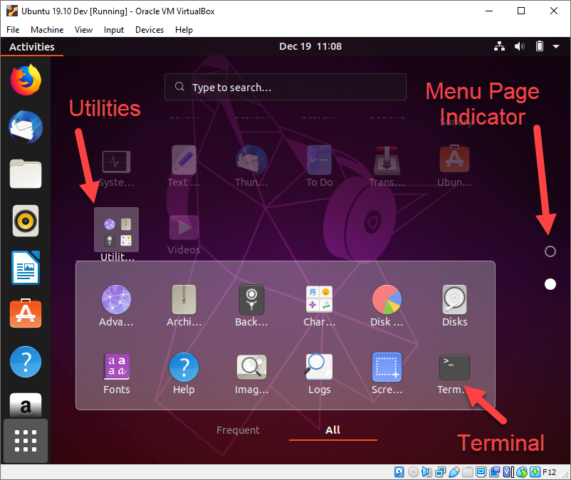
Over to the right is the Menu Page Indicator. The number of menu pages is dependent upon how many applications you have installed and the size of your screen. In the above screenshot the Menu Page Indicator shows I have two pages of menus; there will be a dot for each page and the solid dot indicates I am on the second page.

To get to the terminal, find the box labeled Utilities. This is a submenu, when you click on it the Utilities expands, and in it you’ll find the icon for the Terminal.

There is a second method for getting to the terminal that you could use. Many Linux distros have a built-in keyboard shortcut to launch the terminal, in Ubuntu CTRL+ALT+T will launch a new terminal window. Other distros use the Superkey+T shortcut, where superkey would be the Windows key on many keyboards. No matter which way you choose, it’s now time to open up a terminal window and continue our setup of Ubuntu.

Apply Updates

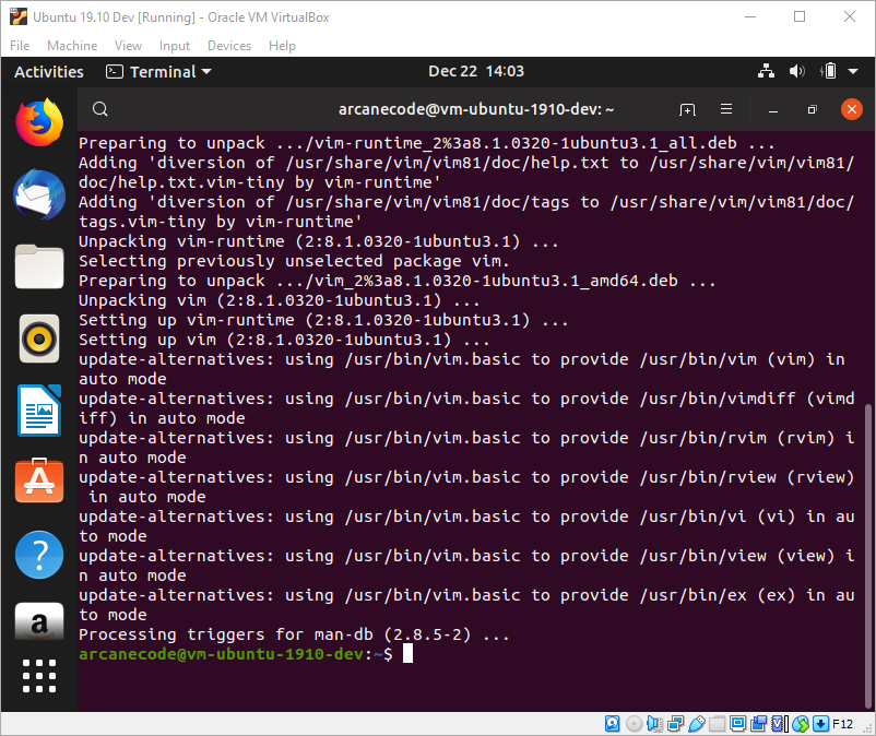
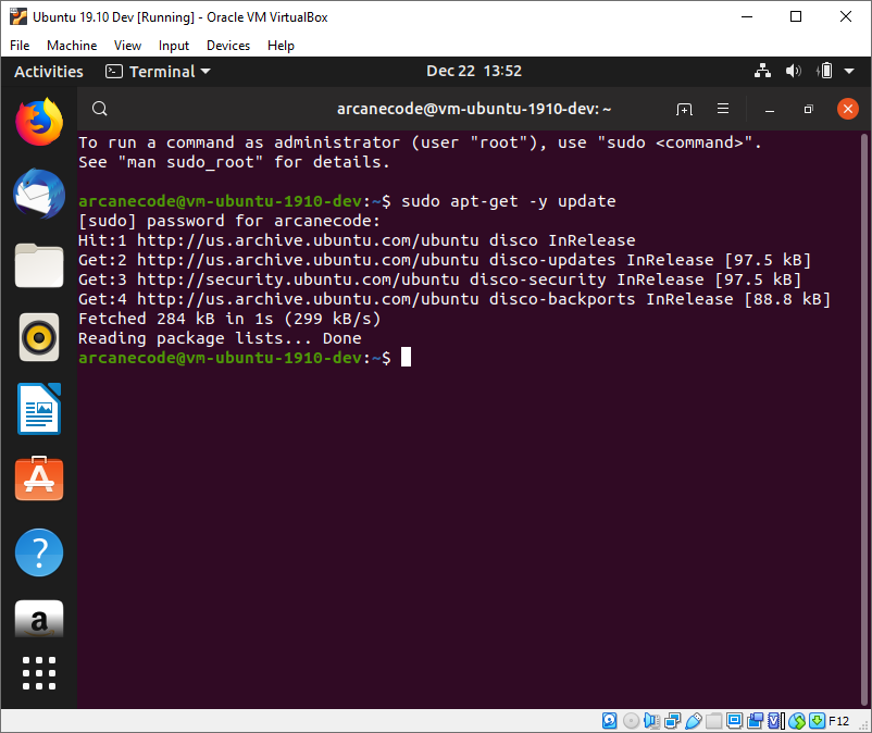
Before proceeding, you should first apply any new updates. Doing so is very easy, at the terminal window enter the following command.

sudo apt-get -y update

The sudo command is short for Super User DO; it is the equivalent of “Run as Administrator” in Windows. When you enter a command using sudo you’ll be prompted for your password. If you enter more sudo commands, Linux will remember your recently entered password for a brief time so you don’t have to keep reentering it.

The apt in apt-get stands for Advanced Package Tool. It, as well as the apt command you’ll see in a moment, is part of a suite of tools used to install new applications or keep your system up to date. In order to understand how this works, you need to understand how Linux manages packages. Each Linux distro maintains its own set of package repositories. Think of it as a sophisticated lookup tool. When you issue an apt command to go get application “X”, your operating system looks in its library for “X”. It has an entry to go to a specific location on the internet, where application “X” can be downloaded, along with any special instructions for installation. Note the apt commands can also be used for more than just applications. It may also be used to install operating system updates, as in the above example, or to upgrade your operating system to a more recent version.

It is also possible to add additional repositories to your distro. Many companies provide their own set of package repositories with which you can use the apt commands to install and update their specific applications.

Returning to the syntax of the command, the -y tells the apt-get command to automatically reply yes to any “are you sure” style prompts. Finally, the update tells apt-get to make sure all operating system components and applications are up to date.

Now that you understand the basic syntax of the command, enter it and press enter. You’ll be prompted to enter your password, do so and the update process will begin.

Install Additional Utilities

There are a few utilities that you may need as you work with Ubuntu over time. While you won’t necessarily use these during this course of articles, they are common to many developer installs. As you read through other tutorials here on Red Gate’s Simple Talk site as well as other locations, it will be assumed you have these already installed. As such, I go ahead and install these as part of my developer installs and suggest you do so, too.

VIM

First, install a basic text editor called VIM. VIM works in the terminal and makes it easy to edit text files. To do so, use the apt command just discussed.

sudo apt -y install vim

Note this code is using only the apt command, not apt-get. It’s also using install to indicate you are installing a new application, and vim is the name of the application to install.

This would be an opportune time to mention that Linux is case sensitive. If I had used VIM instead of vim in the above example, the apt command would have failed.

This also applies to file and directory names. For example, myfilename.txt, MYFILENAME.TXT, and MyFileName.txt refer to three different files, and all three could exist in the same folder.

net-tools

Having a set of network tools can be handy to do things such as discover your network status and information. Those are found in a suite of tools called net-tools. To install, use the following command.

sudo apt -y install net-tools

Once it has installed, you can use the command ifconfig to test it, ifconfig will display your network configuration.

As you can see, ifconfig returns quite a bit of useful information about our machine’s network info.

Git

Many developers use a code repository to store the source code to their applications. A code repository is a bit different than the Linux repositories you’ve seen so far in this article. Those repositories are used to hold installable applications. The git repositories are used to hold the source code needed to build those applications.

Git is one flavor of a repository. It can be hosted locally, within your own company, or on a platform. GitHub is probably the most popular of these and can host both public and private repositories for free. As it is used so much, I go ahead and install in every developer system I set up.

sudo apt -y install git-all

By now most of this command should be familiar to you, git-all is the application name that will install all the git components.

Once installed, you can enter the command git to confirm it was installed. It will show you the basic help for the git application.

Snap

The apt command is not the only method by which you can download and install applications. The two most popular in the Linux community are flatpacks and snaps. Ubuntu favors the snap method, and the most recent versions of Ubuntu already have the snap application installed. To see if you have it, simply enter the command snap in the terminal and press enter.

Should you get the error message that snap was not found, you can install it by using apt.

sudo apt -y install snapd

Two things to note, first that is not a misspelling in the command, snapd is the name of the application to use. Second, snaps are only supported on Ubuntu versions 18.04 and later.

Conclusion

This article covered the first steps in setting up a development environment for developing PowerShell Core scripts in a Linux environment, specifically Ubuntu. It described using VirtualBox as the virtual machine manager, downloaded Ubuntu, and configured VirtualBox for a new Ubuntu install. With minor modifications, you could have also adopted the instructions for Hyper-V, or set up an empty PC with Ubuntu running “bare metal”, right on the computer itself.

It then covered installing Ubuntu 19.10, stepping through each screen in the installation process and discussing the options, allowing for choices when installing in a virtual machine versus a real computer. After installing, you logged in, updated Ubuntu, and then added several small utilities such as VIM and the networking tools.

In part 2 of this series, I’ll demonstrate installing PowerShell Core and Visual Studio Code. In addition, you will learn how to install Azure Data Studio to prepare for future database work. I’ll wrap up part 2 by automating the update to the favorites bar, configuring it for a development centric environment.

This foundation is a good position for growth. I’ll expand on the base created in parts 1 and 2 in future articles, including one on installing SQL Server in a Docker container on Linux.

The post How to Create an Ubuntu PowerShell Development Environment – Part 1 appeared first on Simple Talk.


from Simple Talk https://ift.tt/2ugK2um
via