Monday, February 10, 2020

Why Empathy is Not Enough in Tech

In 2020, my main personal goal is to reduce doing harm, and this has been mainly inspired by the work of Kim Crayton and the #causeascene Guiding Principles. Kim is a business strategist, tech leader coach, professional educator, and founder of the #causeascene movement.

Tech is not neutral.

Actually, it has never been neutral, nor has it been apolitical. While we, as developers, want to believe differently, the news is full of examples of how tech has been and is continuously used to harm people, especially the ones that are already most vulnerable:

  • Careless or intentionally malicious handling of private data (Facebook)
  • Nonconsensual use of Profile picture to use as (flawed and insecure) face recognition (AirBnB)
  • Tech companies using their products to spy on employees and shut down protests (Google)
  • Racism and sexism built directly into AI algorithms (Amazon)
  • Social Media being used to harass and shutdown members of marginalized groups, spread fake-news and amplify hate

But it doesn’t stop at the big tech companies; harm is being done on all levels, be it the language used by technologists (“If you don’t get this, you have no business in coding”, “Problem exists between keyboard and chair”), the bias in hiring process (“Not a culture fit”) or the use of racist terms and “jokes” under the coat of freedom of speech.

These harmful actions, processes, and policies have come at great cost for teams, the trade as such, and also its products.

It has led to an artificially narrowed pool of “talent” and therefore also a narrowed viewpoint, rendering many tech companies unable to predict the potential harm their products and services are causing.

Luckily, there’s empathy and compassion – let’s assume we have good intentions, and if we try hard enough to walk in each other’s shoes, we’ll be able to solve all the problems we don’t even know exist. How hard can it be to imagine how a black woman in her 50s from the other side of the globe will use our software. As a white man in my 30s, I just must be empathetic enough, right?

In fact, we’re not even able to be empathetic enough to create soap dispensers or fitness trackers that work on non-white skin tones.

Don’t get me wrong – empathy is a great skill to develop, but it can never be a replacement for authentic lived experience. The only chance to really broaden our views is to introduce diversity into our teams, and to be able to do so, we need to become inclusive. Focusing on being compassionate won’t do it if we don’t develop a clear strategy.

“The road to hell is paved with good intentions”

If we want to stop doing harm, we need to create strategies that allow us to focus on the impact of our actions. We need strategies that allow us to learn what impact our actions have on people different than us, what (unintended) side-effects our actions have, how our work can be used in ways we don’t wan,t and how we can learn and improve from mistakes we made.

Commentary Competition

Enjoyed the topic? Have a relevant anecdote? Disagree with the author? Leave your two cents on this post in the comments below, and our favourite response will win a $50 Amazon gift card. The competition closes two weeks from the date of publication, and the winner will be announced in the next Simple Talk newsletter.


The post Why Empathy is Not Enough in Tech appeared first on Simple Talk.


from Simple Talk https://ift.tt/2w7JZSv
via

But the Database Worked in Development! Checking for Duplicates

The series so far:

Like all grownup database developers, you will do your best to ensure that there are unique constraints and unique indexes in place to prevent duplicates ever getting into the database. These checks are essential, and the RDBMS requires very little effort to make the check when data is inserted. Unless you are working with a very good business analyst, you’ll always miss a few when you create a database, so the addition or alteration of these duplicate checks are an essential part of database maintenance.

Where you were able to do development work on the actual production database, you could check and remove existing duplicates, before you added these constraints, and then provide a data-migration script to go with the deployment. Nowadays, it is more awkward. You’ll probably be required to work on masked data or entirely generated data. You cannot check data if it isn’t exactly what is on production, and it is difficult to predict what could be lurking in the production data.

Now, you have to do all your development work on the constraints and rely on someone else to run the code to remove the duplicates. This is potentially awkward, unless you change your habits to allow easier cooperation between teams. You can, however, very easily generate the code to do these checks, and, even if someone else runs the code, have enough detail about the offending rows to be able to correct the data in a migration script, which can be tested by Ops people on staging.

The same applies to an automated build process. When you’re building a database and then loading in data, it’s much better to check a dataset before constraints are enabled. Once again, what you need is a test script that runs the checks and reports on all the offending rows and only enables constraints if there is no data that would cause an error.

The first article in the series went over the principles of how you might do this as part of a deployment process, with check constraints. Now we move on to checking for duplicates, as defined by your unique indexes.

Reporting on what must be unique in a database

To determine what is defined as being unique in a database, you need to look at both unique constraints that cause a unique index to be created automatically, and unique indexes that are declared directly and explicitly. (All code samples in this series can be found on GitHub.)

DROP PROCEDURE IF EXISTS #ListAllUniqueIndexes
GO
CREATE PROCEDURE #ListAllUniqueIndexes
/**
Summary: >
  This creates a JSON list of all the unique indexes in the database. 
  This includes indexes in the database that have been explicitly 
  declared as well as those that have been automatically created 
  to enforce UNIQUE or PRIMARY KEY constraints
Author: Phil Factor
Date: 12/12/2019
Example:
   - DECLARE @OurListOfUniqueIndexes  NVARCHAR(MAX)
     EXECUTE #ListAllUniqueIndexes 
            @TheJsonList=@OurListOfUniqueIndexes OUTPUT
     SELECT @OurListOfUniqueIndexes AS theUniqueIndexes
   - DECLARE @OurListOfUniqueIndexes  NVARCHAR(MAX)
     EXECUTE #ListAllUniqueIndexes 
            @TheJsonList=@OurListOfUniqueIndexes OUTPUT
     SELECT * FROM OpenJson( @OurListOfUniqueIndexes) 
     WITH (columncount INT, indexname sysname, 
           thetable sysname, columnlist NVARCHAR(4000)
           ,delimitedlist nvarchar(4000))
Returns: >
  the JSON as an output variable
**/
@TheJSONList NVARCHAR(MAX) OUTPUT
AS 
SELECT @TheJSONList=
 (SELECT Count(*) AS columncount, IX.name AS indexname,
        QuoteName(Object_Schema_Name(IX.object_id)) + '.'
        + QuoteName(Object_Name(IX.object_id)) AS thetable,
        String_Agg(QuoteName(col.name), ',') AS columnlist,
        ''''+String_Agg(Replace(col.name,'''',''''''),''',''')+'''' 
               AS delimitedlist
        FROM sys.tables AS tabs
          INNER JOIN sys.indexes AS IX
            ON IX.object_id = tabs.object_id
          INNER JOIN sys.index_columns AS IC
            ON IC.index_id = IX.index_id AND IC.object_id = IX.object_id
          INNER JOIN sys.columns AS col
            ON col.column_id = IC.column_id 
            AND col.object_id = IC.object_id
        WHERE is_unique = 1 -- we only need the ones that 
        --force uniqueness we've chosen to test both the enabled 
        --ones and the disabled ones
        --AND Is_disabled=0
        GROUP BY IX.index_id, IX.object_id, IX.name FOR JSON AUTO)
GO
We can then execute it like this:
DECLARE @OurListOfUniqueIndexes NVARCHAR(MAX);
EXECUTE #ListAllUniqueIndexes 
       @TheJSONList = @OurListOfUniqueIndexes OUTPUT;
SELECT @OurListOfUniqueIndexes;

Note that we’ve chosen to comment out the line that delivers just the enabled constraints. It is a matter of choice, but if an index is there and disabled, I regard it with a certain suspicion.

This will produce a JSON report like this (I’ve just included a few rows):

[
 {
  "columncount": 1,
  "indexname": "PK_SalesTaxRate_SalesTaxRateID",
  "thetable": "[Sales].[SalesTaxRate]",
  "columnlist": "[SalesTaxRateID]",
  "delimitedlist": "'SalesTaxRateID'"
 },
 {
  "columncount": 2,
  "indexname": "AK_SalesTaxRate_StateProvinceID_TaxType",
  "thetable": "[Sales].[SalesTaxRate]",
  "columnlist": "[StateProvinceID],[TaxType]",
  "delimitedlist": "'StateProvinceID','TaxType'"
 },
 {
  "columncount": 1,
  "indexname": "AK_SalesTaxRate_rowguid",
  "thetable": "[Sales].[SalesTaxRate]",
  "columnlist": "[rowguid]",
  "delimitedlist": "'rowguid'"
 },
 {
  "columncount": 2,
  "indexname": "PK_PersonCreditCard_BusinessEntityID_CreditCardID",
  "thetable": "[Sales].[PersonCreditCard]",
  "columnlist": "[BusinessEntityID],[CreditCardID]",
  "delimitedlist": "'BusinessEntityID','CreditCardID'"
 },
 {
  "columncount": 3,
  "indexname": 
       "PK_PersonPhone_BusinessEntityID_PhoneNumber_PhoneNumberTypeID",
  "thetable": "[Person].[PersonPhone]",
  "columnlist": "[BusinessEntityID],[PhoneNumber],[PhoneNumberTypeID]",
  "delimitedlist": "'BusinessEntityID','PhoneNumber'
        ,'PhoneNumberTypeID'"
 }
]

This is one of the reports that I do routinely after a successful build and before data is loaded. This JSON file will usually become part of the build package during deployment. In a sense, it is part of the documentation of the database.

We need to check the data, and report on all the tables and their duplicate rows. We do this after it is loaded and before constraints are enabled. If we are doing a release by synchronizing with an existing version of the data, it is done by synchronizing with a version of the database that has its constraints disabled, and before a post-deployment script enables them.

We can, of course, generate the report and then use it immediately. We do this if we have built the database, ensured that constraints are disabled and then loaded the data.

Here is a batch that produces a JSON report. The batch not only checks for duplicates in the data but also checks that the table and columns mentioned in the constraint exist. If it can’t run the test because the columns aren’t there, then it reports the fact. It makes as few assumptions as possible.

Note that this script must be checked with your security team because actual data for the relevant columns of duplicate rows is stored in the resulting report. There is no way around this, but the risks of ‘leakage’ are low, and you get to be able to keep almost all sensitive data at arm’s length.

I’ve now got this all wrapped up in a temporary stored procedure TestAllUniqueIndexes.sql which is available on Github.

DECLARE @OurListOfUniqueIndexes NVARCHAR(MAX);
EXECUTE #ListAllUniqueIndexes 
        @TheJSONList = @OurListOfUniqueIndexes OUTPUT;
DECLARE @TheUniqueIndexes TABLE --the list of unique 
    --indexes in the database
  (
  TheOrder INT IDENTITY PRIMARY KEY,--needed to iterate 
         --through the table
  ColumnCount INT, --the number of columns used in the index
  IndexName sysname, --the name of the index
  TheTable sysname, --the quoted name of the table with the schema
  ColumnList NVARCHAR(4000), --the list of columns in the index
  DelimitedList NVARCHAR(4000) --the list of columns in the index
 );
INSERT INTO @TheUniqueIndexes (ColumnCount, IndexName, 
        TheTable, ColumnList, DelimitedList)
  SELECT * FROM OpenJson(@OurListOfUniqueIndexes)
  WITH
    (columncount INT, indexname sysname, 
     thetable sysname, columnlist NVARCHAR(4000)
     ,delimitedlist nvarchar(4000)
  );
DECLARE @Breakers TABLE (TheObject NVARCHAR(MAX));
DECLARE @Errors TABLE ([Description] NVARCHAR(MAX));
DECLARE @Duplicates NVARCHAR(MAX); ---list of duplicate rows 
DECLARE @ExecString NVARCHAR(MAX); --The string for that finds 
                                   --the duplicates
DECLARE @indexName sysname; --to hold the value when iterating 
                            --through the result
DECLARE @tablename sysname; --to hold the value when iterating 
                            --through the result
DECLARE @CheckExecString NVARCHAR(MAX); --The string for that 
                                        --checks the cols exist
DECLARE @columnList NVARCHAR(4000); --to hold the value when iterating 
                                    --through the result
DECLARE @columnDuplicates NVARCHAR(MAX);--the duplicate indexes
DECLARE @AllColumnsAndTableThere int
DECLARE @iiMax INT = @@RowCount;
DECLARE @ii INT = 1;
WHILE (@ii <= @iiMax)
  BEGIN
    SELECT @CheckExecString ='SELECT @AllColumnsThere =
  CASE WHEN '+Convert(varchar(3),ColumnCount)+' =
  (
  SELECT Count(*) FROM sys.columns AS c
    WHERE c.name IN ('+delimitedList+')
      AND Object_Id('''+TheTable+''') = c.object_id
  ) THEN 1 ELSE 0 END;
', @ExecString =
      N'SET @duplicates=(SELECT top 50 Count(*) AS duplicatecount, '
      + ColumnList + N' FROM ' + TheTable + N' GROUP BY ' + ColumnList
      + N' HAVING Count(*) >1 FOR JSON auto)', @indexName = IndexName,
      @tablename = TheTable, @columnList = ColumnList
      FROM @TheUniqueIndexes
      WHERE TheOrder = @ii;
    EXECUTE sp_executesql @CheckExecString, 
              N'@AllColumnsThere int output',
      @AllColumnsThere = @AllColumnsAndTableThere OUTPUT;
    if @AllColumnsAndTableThere=1
      BEGIN
      EXECUTE sp_executesql @ExecString, 
              N'@duplicates NVARCHAR(MAX) output',
        @duplicates = @columnDuplicates OUTPUT;
       IF @columnDuplicates IS NOT NULL
        INSERT INTO @Breakers (TheObject)
          SELECT
            (
            SELECT @indexName AS indexName, 
              @tablename AS tablename,
              @columnList AS columnlist, 
              Json_Query(@columnDuplicates) AS duplicates
            FOR JSON PATH, WITHOUT_ARRAY_WRAPPER
            );
      END
    ELSE
       INSERT INTO @errors(description) 
         SELECT 'Table' + @Tablename
                +'either didn''nt exist or didn''t have the column(s)' 
                +@columnlist+ 'so index '+@Indexname+' was untested'
    SELECT @ii = @ii + 1; --do the next unique index in the list
  END;
SELECT (SELECT Json_Query(TheObject) AS duplicated 
        FROM @Breakers FOR  JSON auto) AS duplicatelist,
       (SELECT description FROM @Errors FOR JSON auto) AS errors 
       FOR JSON path;

Testing it out: finding duplicate rows in AdventureWorks

Well, this is all pretty straightforward, but we need to be able to test it. We’ll take poor old AdventureWorks2016, which has some tables that are very handy for the purpose. The Sales.SalesTaxRate table has two unique indexes on top of its surrogate primary key. One of them, AK_SalesTaxRate_rowguid , ensures that the rowguid is unique: The other one, AK_SalesTaxRate_StateProvinceID_TaxType, ensures that there is only one tax rate for any Sales Tax rate, tax type and location. We can try introducing a duplicate:

--disable all constraints
ALTER TABLE Sales.SalesTaxRate NOCHECK CONSTRAINT ALL;
--disable the unique constraints that aren't used as a primary key
ALTER INDEX AK_SalesTaxRate_StateProvinceID_TaxType 
      ON Sales.SalesTaxRate DISABLE;
ALTER INDEX AK_SalesTaxRate_rowguid ON Sales.SalesTaxRate DISABLE;
--deliberately create a duplicate 
INSERT INTO Sales.SalesTaxRate (StateProvinceID, TaxType, TaxRate, 
      Name, rowguid, ModifiedDate)
  SELECT StateProvinceID, TaxType, TaxRate, Name, rowguid, ModifiedDate 
  FROM Sales.SalesTaxRate
  WHERE SalesTaxRateID = 1;

This works because we’ve deliberately disabled the checks before we introduced a duplicate. We can test this by enabling the indexes:

--enable the unique indexes
ALTER INDEX ALL ON Sales.SalesTaxRate REBUILD;
--at this point there is an error
/*
Msg 1505, Level 16, State 1
The CREATE UNIQUE INDEX statement terminated because a duplicate key 
was found for the object name 'Sales.SalesTaxRate' and the index name 
'AK_SalesTaxRate_StateProvinceID_TaxType'. 
The duplicate key value is (1, 1).
*/

So, we’ve now confirmed that this data will trigger an error in a build if we enable the unique constraints and indexes. We can now run the code to check all the tables in the database. Before we do this, however, here’s the code you can run after your tests to return AdventureWorks to its former state:

--we can do this to recover the table
DELETE FROM [Sales].[SalesTaxRate] WHERE SalesTaXrateID>29
--enable the unique indexes
ALTER INDEX ALL ON Sales.SalesTaxRate REBUILD;
--enable constraints
ALTER TABLE Sales.SalesTaxRate WITH CHECK CHECK CONSTRAINT ALL;

Running TestAllUniqueIndexes.sql produces a JSON report that tells us how to fix the problem.

[
  {
    "duplicatelist": [
      {
        "duplicated": {
          "indexName": "AK_SalesTaxRate_StateProvinceID_TaxType",
          "tablename": "[Sales].[SalesTaxRate]",
          "columnlist": "[StateProvinceID],[TaxType]",
          "duplicates": [
            {
              "duplicatecount": 2,
              "StateProvinceID": 1,
              "TaxType": 1
            }
          ]
        }
      },
      {
        "duplicated": {
          "indexName": "AK_SalesTaxRate_rowguid",
          "tablename": "[Sales].[SalesTaxRate]",
          "columnlist": "[rowguid]",
          "duplicates": [
            {
              "duplicatecount": 2,
              "rowguid": "683DE5DD-521A-47D4-A573-06A3CDB1BC5D"
            }
          ]
        }
      }
    ]
  }
]

This JSON report has two parts, the duplicate list and the errors. We can breathe a sigh of relief that there is no error list, which would mean that the database has changed enough that either columns or tables have changed their name. There are two duplications in the list, because two unique indexes have been compromised by the row we inserted. The report tells you what values were duplicates from the perspective of the unique constraint being checked

This information is intended to give the developer enough information to provide a script that corrects the data, but it will need to be tested on a database that has a good realistic generation of data so you can run tests that ensure that only the duplicate rows are affected by your corrections.

Automating the process

Because we’ve kicked into touch the problem of inputs and outputs from procedures by using JSON, we can simplify the process. I’ve designed a process that does as many setup and tear-down SQL files as you need, and which will do the following three essential processes:

  1. Check the new database after loading the data, but before the constraints and indexes are enabled. This runs a check that will tell you what you need to fix and put these into a report, for every database you specify on every server you specify. I realise that things start with just one database on one server but tend to escalate.
  2. Report on the constraints of a database. Check constraints, unique constraints and foreign key constraints are all reported on separately, in a file. The most important message was whether everything was OK, but all potential breaches of the proposed constraint are reported along with errors in the process
  3. Use the report on the constraints to run checks on the data in the specified database.

Logically speaking, processes 2 and 3 are components of process 1. However, you are not always lucky enough, as a developer, to be in charge of loading and checking the data all in one process. Having them as two different processes gives you more flexibility to fit in with the deployment regime.

What we’ve done is to design stored procedures for testing, or gathering data for, the various constraints. Because they all take JSON input and JSON output, we can radically simplify the PowerShell script we use to do the checks. We must keep with a common convention for alerting the user to the presence of rows that would trigger constraint errors if constraints were enabled, and we need a common way of advising if we can’t even run the test.

Because there are a lot of files and code, I’ve created a GitHub site with all the code in it here.

Summary

There are two points in any build, test or deployment where you can get into difficulties with your data because you have duplicates, bad data or data that has lost its relational integrity. Firstly, when you do a build, disable constraints temporarily and Load (BCP) in the data, and secondly, when you synchronize with a version of the database that does more checking of the data. If you have existing bad data, you need a way of fixing it. To do that, you need to know about the data that would fail the constraint tests that your constraints would use if they were enabled.

We need a slightly different ways of testing Check constraints (bad data checks), Unique Constraints (duplicate checks) and Foreign Key constraints (relational integrity checks). We can store the list of constraints from the source database as a JSON file, and we can take this list as a source and store the result of our tests in a JSON report file

To run all these tests in a flexible way that fits in with a wide range in methods of deployment, I’ve devised a general-purpose data-driven way of running these tests and reports in PowerShell.

In my final article I’ll describe how to check foreign key constraints


The post But the Database Worked in Development! Checking for Duplicates appeared first on Simple Talk.


from Simple Talk https://ift.tt/2upTWKE
via

Tuesday, February 4, 2020

Key Findings from the 2020 Database DevOps Survey

Each year Redgate Software runs a survey to learn more about how organizations practice DevOps, especially when it relates to the database. This year, over 2000 individuals responded, and they are from diverse industries and company sizes.

The key findings in the report are:

  • Frequent database deployments are increasing: 49% of respondents now report they deploy database changes to production weekly or more frequently.
  • Frequent deployers who use version control report lower production defect rates.
  • Respondents who report that it is easy to get a code review for database changes report lower production defect rates and lower lead time for change deployment.
  • Although 38% of responders report the use of Change Approval Boards, we see no evidence that Change Approval Boards lower code defect rates, only that they increase lead time for changes.
  • Respondents who reported that all or nearly all their database deployments take place with the system online also reported lower lead time for changes and lower defect rates.
  • 60% of Enterprise respondents believe the move from traditional database development to a fully automated process for deployment can be achieved in a year or less. 66% in non-Enterprises believe this can be accomplished.

As I read through the report, one thing stood out to me: organizations who deploy more frequently have lower defect rates. In fact, “37% of those who have adopted DevOps across all projects report that 1% or less of their deployments introduce code defects which require hotfixes, compared to 30% for all other groups.”

When there is a defect in software, it’s usually easy to rollback changes. Maybe services must be reconfigured, or files replaced. Deployment issues with databases are much more critical and difficult to resolve. Typically, you can’t just do a restore of production because of data loss, and the database will not be available during the restore.

Instead of massive changes every few weeks or months, small changes are deployed frequently with DevOps. Frequent database changes do sound intimidating, but because these are small changes, there is less of an impact on stability. And that reported decrease in defect rates from 30% to 1% is impressive!

Even if your company is not “all in” yet, there are things you can do. Make sure that you are using source control to keep track of database changes. Begin automating database deployments to dev and other non-production environments. Make an effort to communicate with other teams to break down those silos.

There’s a lot to learn from the report, and I hope you take a look and consider participating in next year’s survey.

Commentary Competition

Enjoyed the topic? Have a relevant anecdote? Disagree with the author? Leave your two cents on this post in the comments below, and our favourite response will win a $50 Amazon gift card. The competition closes two weeks from the date of publication, and the winner will be announced in the next Simple Talk newsletter.


The post Key Findings from the 2020 Database DevOps Survey appeared first on Simple Talk.


from Simple Talk https://ift.tt/393ZKb7
via

Monday, February 3, 2020

Text Mining and Sentiment Analysis: Introduction

Text Mining and Sentiment Analysis can provide interesting insights when used to analyze free form text like social media posts, customer reviews, feedback comments, and survey responses. Key phrases extracted from these text sources are useful to identify trends and popular topics and themes. Sentiment scores provide a way to perform quantitative analysis on text data. Combining these techniques, using visually engaging dashboards will help unlock the value of your text data.

This three-article series about Text Mining and Sentiment Analysis will start with exploring Azure Cognitive Services -Text Analytics APIs. In the second article, I’ll discuss various qualitative and quantitative techniques to analyze the data and create compelling visualizations in Power BI. The third and final article of this series will show how to use R to generate a Word Cloud, sentiment scores and NRC sentiment.

NOTE:These articles assume basic familiarity with Power BI and Azure.

Introduction

Have you looked at social media posts, customer reviews and feedback, survey responses to open-ended questions, or pretty much any free form text and wondered about analyzing that data? Maybe you have tried analyzing this type of data with R or Python and wondered if you are using the right lexicon or library for the task. Have you wondered about how to visualize the outcome of such analysis, create Dashboards and share it with relevant people in your company? You can use Power BI and Azure Cognitive services, to perform these tasks – no advance programming expertise or guru level of technical knowledge needed!

The Text Analytics API is a part of Azure Cognitive Services, a collection of machine learning and AI algorithms in the cloud. It provides advanced natural language processing of raw text, and includes four types of analysis:

Sentiment analysis returns a sentiment score between 0 and 1 for each set of text, where 1 is the most positive and 0 is the most negative score. It is useful to find out what customers think of your brand or topic by analyzing raw text for clues about positive or negative sentiment. The analysis models are pretrained using an extensive body of text and natural language technologies from Microsoft. For selected languages, the API can analyze and score any raw text that you provide, directly returning results to the calling application.

Key phrase extraction – extracts a list of important words and phrases, for each document and is used to identify the main points, themes, and topics in your text. For example, for the input text “I had a wonderful trip to Seattle for a conference”, the API returns the main talking points: “wonderful trip”, “Seattle” and “conference”.

Language detection – can recognize a wide range of languages, variants, dialects, and some regional/cultural languages. It detects the language of the input text and returns a single language code (paired with a score indicating the level of confidence) for every document submitted on the request

Named Entity recognition – identifies and categorized various entities in the input text as places, people, organizations, currencies, date/time, etc. Well-known entities are recognized and linked to more information on the web.

Each of these operations may work with different languages. While the services support English for all operations, you will find a full and updated list of languages supported for various Text Analytics operations here.

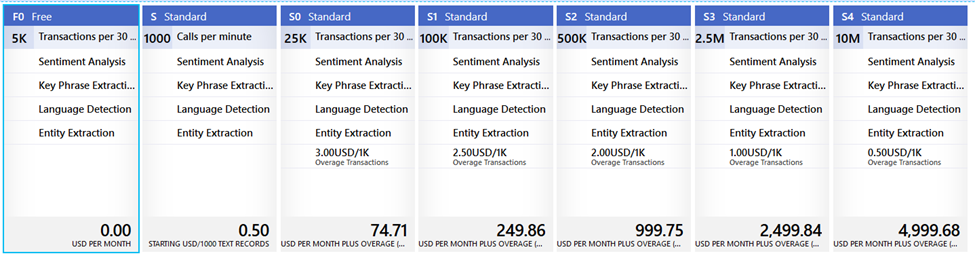
All Text Analytics API Endpoints (operations) accept raw text data, commonly referred to as a document. The current size limit for each document is 5,120 characters, so you must break down any larger documents into smaller chunks for analysis. The number of requests processed per second or minute (rate limit) depends on your pricing tier. These pricing tiers start from the F0 Free tier (which allows five thousand transactions per month at no cost), going up to the S4 Standard tier (which allows ten million transactions per month for about 5,000 USD and charges 0.50 USD per one thousand transactions over that limit).

A picture containing screenshot, wall Description automatically generated

Figure 1. Azure Text Analytics pricing tiers

Please note that your bill will depend on your actual usage, in addition to the selected pricing tier. You can find additional details about Cognitive Services pricing here and details about the data limits for each pricing tier here.

Text Analytics Containers (these are standard Docker containers) allow you to run the Text Analytic APIs in your own environment, to meet your specific security and data governance requirements. These containers will not send any customer data to Microsoft. Only billing information is sent to Azure, using a Text Analytics resource on your Azure account.

Key Phrases and Sentiment Scores

Key Phrases and Sentiment Scores allow performing both qualitative and quantitative analysis on this data. Qualitative data consists of text – words and narratives. Analysis of this data includes extraction of key phrases and counting word frequency, identifying themes and highlighting concepts. While qualitative data analysis can be time-consuming and somewhat subjective, it can help provide a nuanced understanding of the survey participants perspectives. Word Cloud is one of the most popular ways to visualize Key Phrase frequency analysis. The next article in the series will explore the Word Cloud in detail.

Numeric Sentiment Scores are quantitative data points, extracted from the text. Quantitative data is numeric, and the numbers are clear and specific. You can easily aggregate them, apply filters, make charts and graphs and apply statistical techniques to analyze them. You’ll learn how to create several charts using the sentiment scores in the next article of this series. A combination of qualitative and quantitative techniques is quite useful with a well-rounded analysis and visualization of text data coming from Surveys.

Several options are available for using the Text Analytics APIs;

  • Evaluate Azure Cognitive services for free, as a Guest with a 7 Day Trial
  • Use Azure Cognitive Services for non-production workloads, through your free Azure Account
  • Use Azure Cognitive Services for Production workloads, through your existing enterprise Azure account

You can always give it a try from your browser, using this link.

The following four easy steps will help you get set up for using the Text Analytics APIs to generate key Phrases and Sentiment Scores. The data from the Team Health Survey Results from a fictional company will be analyzed in this article

Step One – Set up an Azure Cognitive Services Resource

Assuming you have an Azure subscription/Account, set up Cognitive Services resource using the Azure Portal.

  1. Sign in to the Azure portal, click +Create a resource. Use the search bar to find text analytics.
  2. Select Text Analytics from the search results and hit the Create button.
  3. On the Create screen, enter the required details (please review the pricing details to choose a pricing tier that best fits your needs) and hit the Create button.
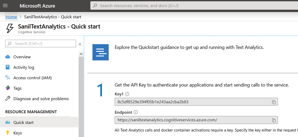
  4. Your deployment will begin and may take a few seconds to complete. Once it’s ready, click to open it and make a note of the Endpoint as well as the Access Keys. You will need them to Integrate Power BI with the Text Analytics Cognitive Service.

Please note that the subscriptions keys are used to access your Azure Cognitive service API and should be treated with the same precautions as you would take for your passwords. Store them securely and do not share them. Azure recommends regenerating these keys regularly for security (like changing your passwords at regular intervals).

A screenshot of a social media post Description automatically generated

Figure 2. Endpoint and Text Analytics API

Step Two – Loading Data into Power BI Desktop

The Team Health Survey data is in an Excel spreadsheet and has four fields:

  • Period (Year & Quarter number)
  • Manager (Name)
  • Team (Name)
  • Response (the free form text responses from the Survey, to the question – How do you feel about your team’s health in this recent quarter)

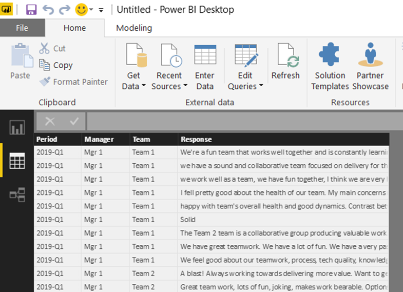
Here’s a sample of the first few rows:

Figure 3. Raw data sample

Launch Power BI Desktop and navigate to the Get Data menu to load the Excel spreadsheet. At this time, you can also perform transformations like changing data types, lengths, precisions, etc. Power BI gives you a preview, using a small sample of the data set. Once loading is complete, you can see the loaded data by clicking on the Data View button on the left edge of the Power BI workspace. If you would like to remove all the extraneous columns, select the four with data, right-click and choose Remove Other Columns.

Figure 4. The loaded data

Step Three – Creating Custom Functions in Power BI

In this scenario, no other data preparation/transformation is needed, so the next step is creating the custom functions that will integrate Power BI and Text Analytics. The function receives the text to be processed as a parameter. It converts data to and from the required JSON format and makes the HTTP request to the Text Analytics API. The function then parses the response from the API and returns a response. Power BI Desktop custom functions are written in the Power Query M formula language, “M” for short. You can learn more about it here.

The solution required two functions:

  1. Key Phrases – which returns a string that contains a comma-separated list of the extracted key phrases.
  2. Sentiment Score – which returns a numeric score ranging from 0 to 1.

In Power BI Desktop, open the Power Query Editor window by clicking Edit Queries on the Home ribbon. Then click New Source Blank Query found on the Home ribbon. A new query will appear in the list – rename it KeyPhrases.

Open the Advanced Editor found in the Query group of the Home ribbon and replace any existing text with the following code. Remember to use your own API Key and Endpoint.

// Returns key phrases from the text in a comma-separated list
(text) => let
    apikey      = "YOUR_API_KEY_HERE",
    endpoint    = "YOUR_ENDPOINT_HERE/text/analytics/v2.1/keyPhrases",
    jsontext    = Text.FromBinary(Json.FromValue(Text.Start(Text.Trim(text), 5000))),
    jsonbody    = "{ documents: [ { language: ""en"", id: ""0"", text: " & jsontext & " } ] }",
    bytesbody   = Text.ToBinary(jsonbody),
    headers     = [#"Ocp-Apim-Subscription-Key" = apikey],
    bytesresp   = Web.Contents(endpoint, [Headers=headers, Content=bytesbody]),
    jsonresp    = Json.Document(bytesresp),
    keyphrases  = Text.Lower(Text.Combine(jsonresp[documents]{0}[keyPhrases], ", "))
in  keyphrases

After saving the KeyPhrases function, follow the same steps and create a SentimentScore function, using the following code in the Advanced Editor window

// Returns the sentiment score of the text, from 0.0 (least favorable) to 1.0 (most favorable)
(text) => let
    apikey      = "YOUR_API_KEY_HERE",
    endpoint    = " YOUR_ENDPOINT_HERE/text/analytics/v2.1/sentiment",
    jsontext    = Text.FromBinary(Json.FromValue(Text.Start(Text.Trim(text), 5000))),
    jsonbody    = "{ documents: [ { language: ""en"", id: ""0"", text: " & jsontext & " } ] }",
    bytesbody   = Text.ToBinary(jsonbody),
    headers     = [#"Ocp-Apim-Subscription-Key" = apikey],
    bytesresp   = Web.Contents(endpoint, [Headers=headers, Content=bytesbody]),
    jsonresp    = Json.Document(bytesresp),
    sentiment   = jsonresp[documents]{0}[score]
in  sentiment

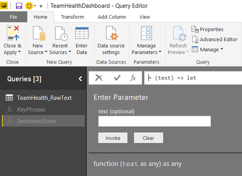
You should now see both custom functions, under Queries on the left-hand side.

Figure 5. Custom Functions in Query Editor Window

Step Four – Invoking the Newly Created Custom Functions

You can now use these custom functions to extract key Phrases and generate a Sentiment Score for each of the text responses and store them as new columns in the Table.

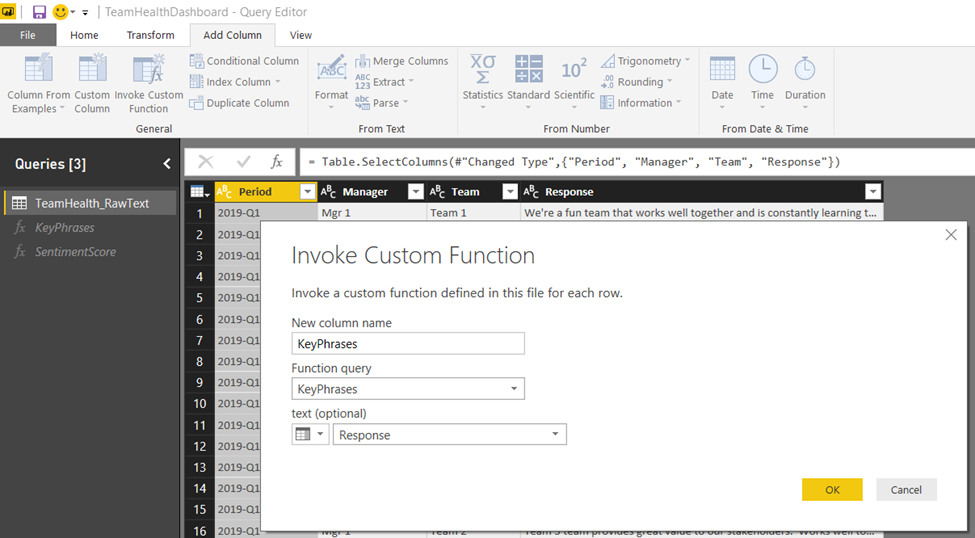
In Power BI Desktop Query Editor window, switch to the TeamHealth_RawText Query and select the Add Column ribbon, then click Invoke Custom Function. The Invoke Custom Function dialog appears. For New column name, enter KeyPhrases. For Function query, select the custom function you created, KeyPhrases. A new field appears in the dialog, text (optional), asking which column to provide as input values for the text parameter of the API. Select Responses from the drop-down menu and click OK.

Figure 6. Invoking the KeyPhrases custom function

After you close the Invoke Custom Function dialog, a banner may appear asking you to specify how to connect to the Key Phrases API. Click Edit Credentials, make sure Anonymous is selected in the dialog, then click Connect. Another banner may appear asking you to provide information about your data sources’ privacy. Click Continue and choose Public for each of the data sources in the dialog and Save. Now Repeat these Invoke Custom Function steps for loading another new column: SentimentScore.

You may want to limit the SentimentScore field to two decimal places. Right-click the column and choose Change Type Decimal Number. Then right-click the column and select Transform Round Round… Specify 2 decimal places.

After closing all the dialog boxes, go to the Home ribbon and click Close & Apply. Power BI will need a few minutes to process these queries.

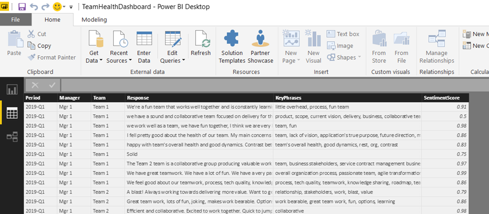
Once all the processing is complete, your Data View will now show the table has been updated with two new fields, that are loaded with KeyPhrases and SentimentScore for each Response text.

Figure 7. Power PI Data View with KeyPhrases and SentimentScore fields loaded

The data table now updated with KeyPhrases and Sentiment scores is ready for use in further analysis and create impactful visualizations in Power BI.

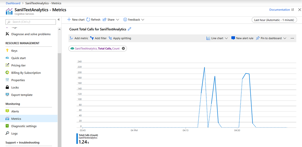
At this time, you can log into the Azure Portal and review the utilization metrics of your Text Analytics Service. You should see a spike in the chart for Total Calls, around the time Power BI was processing your data by invoking the Text Analytics API.

Figure 8. Azure Portal – Utilization Metrics for your Text Analytics Service

Conclusion

This article demonstrated how to do a sentiment analysis using Power BI and Azure Text Analytics. The next article of this three-part series looks at qualitative and quantitative analysis techniques for this data in Power BI. It demonstrates how to create a word cloud, and several statistical charts to help with analyzing this data, extract business value and use Power BI visualizations to narrate a meaningful story about this data.

References:

  • Qualitative or Quantitative Data – https://ift.tt/2GRqOOY
  • Quantitative Data Analysis – https://ift.tt/2UmXVSO
  • Azure Cognitive Services Text Analytics – https://ift.tt/2SdzcNT
  • Power BI Desktop – https://ift.tt/1T1D80M
  • Text Analytics with Power BI – https://ift.tt/2OppRkS


The post Text Mining and Sentiment Analysis: Introduction appeared first on Simple Talk.


from Simple Talk https://ift.tt/2UjXvMT
via

Saving Game Data with Unity

Back in the day, many games had little need for saving data since you could finish a game in about an hour. At best, a game would save a high score and leave it at that. But it didn’t take long for technology to improve, and thus games got longer and more complex. The need for saving all kinds of data, ranging from how much progress the player made in-game or their character’s statistics, became universal whether the game be a simple, linear adventure from beginning to end or it consists of a huge open world. Many games require multiple play sessions to see to the end, and it’s now expected that developers include ways to save the game and come back later. Only when a game is short enough that it can be completed in a single session does the need for saving data diminish, but even in those scenarios, the feature can be very handy.

Unity provides two ways to save a game’s data. They can be quickly described as “the easy way” and “the not so easy way.” The easy way involves Unity’s built-in PlayerPrefs system. Give a value to a key, call Save, and you’re done. On the other hand, the not so easy way involves serializing data and writing to a file for later use. Both methods have their pros and cons, which will be covered as the practices are explored.

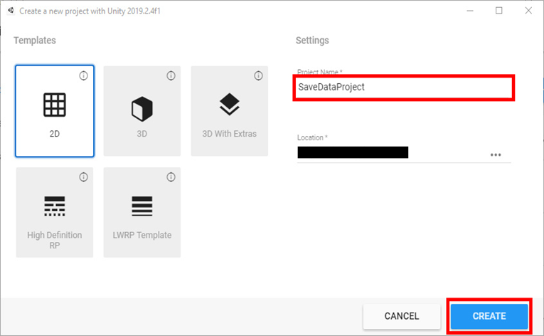
There’s minimal setup involved in testing these out. You just need a project and a couple of scripts. For this project, you will want to use the 2D template for the easiest setup as shown in Figure 1.

Figure 1: Project creation

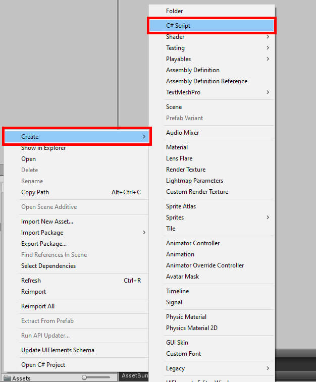
Once you create the project, you’ll need two scripts. You create scripts by right-clicking in the Assets window and selecting Create->C# Script as shown in Figure 2. Call these scripts SavePrefs and SaveSerial.

Figure 2: Script creation

To see what saving a game entails, start with the SavePrefs script. Double-click the script to open Visual Studio.

PlayerPrefs – The Easy Way

To begin, the Start and Update methods can be commented out or deleted as they will not be used to demonstrate the save functionality. Next, some variables to hold the values to save will be needed.

int intToSave;
float floatToSave;
string stringToSave = "";

Next, the OnGui method will create a Graphical User Interface (GUI) from code to manipulate these values. Two buttons created in the method will increase intToSave and floatToSave, and a text field will be made for stringToSave. The code will also create a few labels made to show the current values of these variables. Finally, three more buttons will be made that save, load, and reset data.

void OnGUI()
{
        if (GUI.Button(new Rect(0, 0, 125, 50), "Raise Integer"))
                intToSave++;
        if (GUI.Button(new Rect(0, 100, 125, 50), "Raise Float"))
                floatToSave += 0.1f;
        stringToSave = GUI.TextField(new Rect(0, 200, 125, 25), 
               stringToSave, 15);
        GUI.Label(new Rect(375, 0, 125, 50), "Integer value is " 
               + intToSave);
        GUI.Label(new Rect(375, 100, 125, 50), "Float value is " 
               + floatToSave.ToString("F1"));
        GUI.Label(new Rect(375, 200, 125, 50), "String value is " 
              + stringToSave);
        if (GUI.Button(new Rect(750, 0, 125, 50), "Save Your Game"))
                SaveGame();
        if (GUI.Button(new Rect(750, 100, 125, 50), 
                "Load Your Game"))
                LoadGame();
        if (GUI.Button(new Rect(750, 200, 125, 50), 
                "Reset Save Data"))
                ResetData();
}

The last three buttons all call methods whenever they are clicked, but those methods have not been defined yet. This will be fixed now, starting with the SaveGame method.

void SaveGame()
{
        PlayerPrefs.SetInt("SavedInteger", intToSave);
        PlayerPrefs.SetFloat("SavedFloat", floatToSave);
        PlayerPrefs.SetString("SavedString", stringToSave);
        PlayerPrefs.Save();
        Debug.Log("Game data saved!");
}

No, your eyes do not deceive you. The actual act of saving your game takes only a few lines of code. So, what’s happening? Well, as promised, PlayerPrefs saves the player’s game. First, you must set some variables for PlayerPrefs to save. As seen above, three variables were set, all of them given a name, or key, followed by the variable to save. Once PlayerPrefs is given all its information, Save is called and, as you may have guessed, saves the data. A message is also printed to Unity’s debug console as a little note to the developer saying the save was successful.

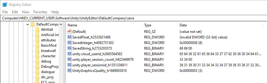
You may be wondering where this save data is on the computer. On Windows, PlayerPrefs can be found in the Registry under HKEY_CURRENT_USER\Software\Unity\UnityEditor\[company name]\[project name] (Figure 3), where company name and project name are names set up in the project settings. Bear in mind this is the location for when the game was run from the editor. In an exe they can be found at HKEY_CURRENT_USER\Software\[company name]\[project name]. On Mac OS, according to the Unity documentation, the PlayerPrefs is found at ~/Library/Preferences folder, in a file named unity.[company name].[product name].plist.

Figure 3: PlayerPrefs variables in the Windows Registry

Loading data is essentially saving data done in reverse. You set your variables of choice to whatever is in PlayerPrefs, and you’re good to go. A good practice is to make sure that the PlayerPrefs for your game has at least one of the keys you’re looking for. In other words, you’re checking that there’s any save data to be found. The code sample below uses HasKey to search for one of the keys declared in the SaveGame method, those keys being SavedInteger, SavedFloat, and SavedString. Looking for just one will be sufficient. So long as PlayerPrefs has one of those, it’s safe to assume it will have the remaining data. Otherwise, it will print an error to the Unity console.

void LoadGame()
{
        if (PlayerPrefs.HasKey("SavedInteger"))
        {
                intToSave = PlayerPrefs.GetInt("SavedInteger");
                floatToSave = PlayerPrefs.GetFloat("SavedFloat");
                stringToSave = PlayerPrefs.GetString("SavedString");
                Debug.Log("Game data loaded!");
        }
        else
                Debug.LogError("There is no save data!");
}

Finally, if you wish to remove the save data stored in PlayerPrefs, all you need to call is PlayerPrefs.DeleteAll and the work is complete. In the following method, DeleteAll is put to use along with resetting the variables and ending by printing a message to the debug console.

void ResetData()
{
        PlayerPrefs.DeleteAll();
        intToSave = 0;
        floatToSave = 0.0f;
        stringToSave = "";
        Debug.Log("Data reset complete");
}

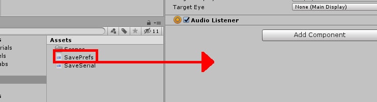
To try it out in-game, save your code and return to the Unity editor. Attach the SavePrefs script to an object, such as Main Camera as shown in Figure 4.

Figure 4: Attaching the SavePrefs script.

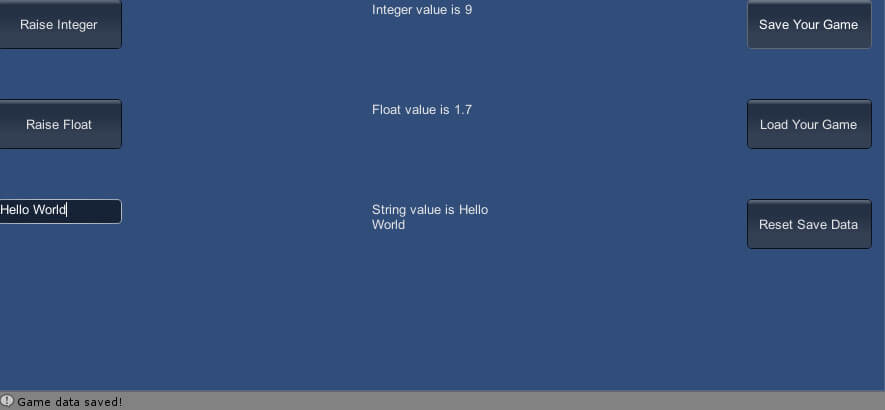
Begin playing the game and tinkering with the GUI on-screen, changing variables to whatever you wish. When ready, save your game. Then try stopping and replaying the game, this time clicking the Load Your Game button. Provided everything works correctly, you should see the variables immediately change to whatever was saved to PlayerPrefs. In addition, you can wipe PlayerPrefs clean by clicking the Reset Save Data button. Figure 5 shows the game in action.

Figure 5: The project in action, using PlayerPrefs

This method seems simple and effective, so why wouldn’t you use PlayerPrefs all the time? Well, PlayerPrefs is one of the least secure ways to save your data, and thus you wouldn’t want to save anything in PlayerPrefs that you absolutely do not want a potential player tampering with. This could be things like how much in-game currency the player currently possesses or stats in a role-playing game. As the name implies, best practices for PlayerPrefs is typically storing a player’s preferences and other trivial data. For example, if you’re letting the user customize the look and size of the game’s UI, PlayerPrefs would be an excellent way to store those preferences.

There’s also the issue of flexibility. The project’s SaveGame method saves an int, float, and string. These are all the data types you can save to PlayerPrefs, so if you wish to save variables of other types, you may be out of luck. Fortunately, there is the “not so easy way” of doing things that allows more flexibility in what you can save, not to mention a little extra security.

Serialization – The Not So Easy Way

Open up the SaveSerial script to begin trying out the next method. Much of the code will be the same as the last script with some minor differences to prove certain points. Here’s the variables and OnGUI method that will be used. All remaining methods will be different.

int intToSave;
float floatToSave;
bool boolToSave;
void OnGUI()
{
        if (GUI.Button(new Rect(0, 0, 125, 50), "Raise Integer"))
                intToSave++;
        if (GUI.Button(new Rect(0, 100, 125, 50), "Raise Float"))
                floatToSave += 0.1f;
        if (GUI.Button(new Rect(0, 200, 125, 50), "Change Bool"))
                boolToSave = boolToSave ? boolToSave 
                       = false : boolToSave = true;
        GUI.Label(new Rect(375, 0, 125, 50), "Integer value is " 
                + intToSave);
        GUI.Label(new Rect(375, 100, 125, 50), "Float value is " 
                + floatToSave.ToString("F1"));
        GUI.Label(new Rect(375, 200, 125, 50), "Bool value is " 
                + boolToSave);
        if (GUI.Button(new Rect(750, 0, 125, 50), "Save Your Game"))
                SaveGame();
        if (GUI.Button(new Rect(750, 100, 125, 50), 
                "Load Your Game"))
                LoadGame();
        if (GUI.Button(new Rect(750, 200, 125, 50), 
                "Reset Save Data"))
                ResetData();
}

To start, a few using statements will be needed to save data using serialization.

using System;
using System.Runtime.Serialization.Formatters.Binary;
using System.IO;

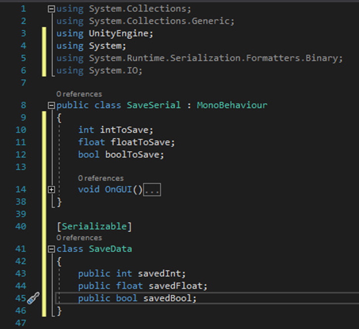
Next, in order to save data, a new class within this script will be created. This class will be made serializable and will consist of the data to be saved.

[Serializable]
class SaveData
{
    public int savedInt;
    public float savedFloat;
    public bool savedBool;
}

I’ve included a screenshot (Figure 6) here to make it easier to understand where this code will go:

Figure 6: SaveSerial script

The goal now is to create the remaining methods that will allow you to save, load, and reset save data. You might notice that the three variables in the SaveData class correspond with the three variables in SaveSerial. Saving data will work by passing SaveSerial's variable values into SaveData and then serializing the SaveData class itself. Returning to the SaveSerial class, create the following method under the OnGUI method.

void SaveGame()
{
        BinaryFormatter bf = new BinaryFormatter(); 
        FileStream file = File.Create(Application.persistentDataPath 
                 + "/MySaveData.dat"); 
        SaveData data = new SaveData();
        data.savedInt = intToSave;
        data.savedFloat = floatToSave;
        data.savedBool = boolToSave;
        bf.Serialize(file, data);
        file.Close();
        Debug.Log("Game data saved!");
}

The BinaryFormatter is used to perform the act of serialization and deserialization. When serializing the data, BinaryFormatter is responsible for converting the information to a stream of 1s and 0s. FileStream and File are used to create a save file with the dat extension under the application’s “persistent data path” followed by any remaining path you wish to make. The persistent data path is C:\Users\[user]\AppData\LocalLow\[company name].

A new instance of SaveData is created, and the variables within SaveData are given the variables in SaveSerial. The BinaryFormatter serializes that data to the file defined in the FileStream. The file is then closed, and a message is printed to the debug console saying the data was saved. Like before, the LoadGame method is very much the same but in reverse.

void LoadGame()
{
        if (File.Exists(Application.persistentDataPath 
                   + "/MySaveData.dat"))
        {
                BinaryFormatter bf = new BinaryFormatter();
                FileStream file = 
                   File.Open(Application.persistentDataPath 
                   + "/MySaveData.dat", FileMode.Open);
                SaveData data = (SaveData)bf.Deserialize(file);
                file.Close();
                intToSave = data.savedInt;
                floatToSave = data.savedFloat;
                boolToSave = data.savedBool;
                Debug.Log("Game data loaded!");
        }
        else
                Debug.LogError("There is no save data!");
}

Your save file by the name of MySaveData.dat is searched for in the same path given in the SaveGame method. Assuming it’s found, it will open the file and deserialize it using BinaryFormatter. Then the variables found in the save file will be fed into SaveSerial's variables. At the end, a message is printed to the debug console saying the load was performed successfully. If there is no file found at the file path, an error message will display instead.

Finally, there’s the act of deleting and resetting save data. This is extremely similar to the PlayerPrefs method but with a couple of extra steps. Unity will first check to make sure there’s a file at the save location before attempting any deleting of files. Assuming there is a file to delete, the variables in this script will also be reset to some default values and a message printed to the console. Like within the LoadGame method, an error message will be printed to the console if there is no file to be found.

void ResetData()
{
        if (File.Exists(Application.persistentDataPath 
                  + "/MySaveData.dat"))
        {
                File.Delete(Application.persistentDataPath 
                          + "/MySaveData.dat");
                intToSave = 0;
                floatToSave = 0.0f;
                boolToSave = false;
                Debug.Log("Data reset complete!");
        }
        else
                Debug.LogError("No save data to delete.");
}

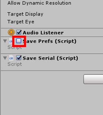
This concludes this script showcasing saving via serialization. Once again, save the code and go back to Unity. Attach SaveSerial to the same object as before and disable the SavePrefs script component.

Figure 7: Disabling the Save Prefs component.

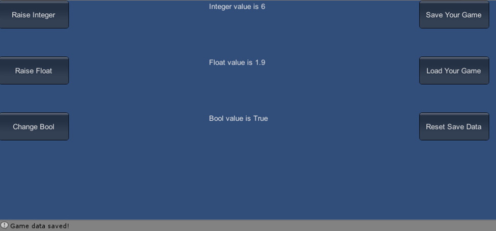
When you run the game, the same UI from earlier appears with some alterations. Tinker with the variables like last time and try saving the game. This time a file is saved to the “persistent data path” of the game, which can be found at C:\Users\username\AppData\LocalLow\project name on Windows and ~/Library/Application Support/companyname/productname on Mac, according to the Unity documentation. Close and reopen the game, then click the load button to bring those values back into the game. And of course, you can delete the saved data entirely if you so desire.

Figure 8: The project in action, using serialization

Conclusion

Barring some very specific exceptions, such as games designed around short play sessions or “perma-death” (perma-death is a game mechanic where once the player loses the game they have to start completely over and everything resets), saving data will be crucial for user retention. Even in those aforementioned examples, most games will at least save a high score or an achievement. What data is saved and how you save that data is down to you and your project’s needs.

Though less secure and limited in what it can save, PlayerPrefs can be helpful for saving a player’s in-game preferences or for games where it doesn’t matter much if the user tinkers with the variables outside the game. In addition, it’s very simple to use which can help save some development time. Meanwhile, serializing data to a file is more complicated but in return, you can save many other types of data and have more security. Like many things in game development, the tools available to you can be utilized in a variety of ways. However, you choose to save your game’s data, there will be options available to you. In the end, the best method is the one that helps you and your project the most.


The post Saving Game Data with Unity appeared first on Simple Talk.


from Simple Talk https://ift.tt/2Ongmmp
via

Saturday, February 1, 2020

Copying of all data between SQL Server databases and servers

This script will copy out all the tables from one version of a database as native BCP format, and  place them in a directory of your choice, (defaulting to your user area in a  directory called BCPFiles). They are placed in sub directories based on your server name and database name, just to keep things neat. It will then if you wish, copy it out to a target server.  On first glance, this routine may seem over-complicated but it is designed to be able to perform this task for a list of these pairs of source & target databases for multi-database  applications if you feel bold. it will allow you to copy the files out just once, and then copy them out to a number of target databases on different servers subsequently. (you determine whether a source or target server is used simply by assigning a $null to $DataSource or $DataTarget when you don’t want the operation to happen).

The script then will transfer this data to an empty version of the same database (same meaning with the same table schema) with no data in it.  If the two versions have a different table structure you’ll get an error. If you use this system and you change the table structure, or constraints, you run your migration code on the source until it is the same as the target.

BCP needs to be installed to run this. This comes with SSMS so you probably have it already. Sometimes you need to create an alias for BCP but I think that problem has gone away

To get started, fill in the connection string for your source of data $datasource and $dataTarget. You also need to fill in an array of objects, each of which define your source and target databases, so you can do a whole list of databases. If you have to use credentials rather than integrated windows security, you add the userID but not the password. You will be asked the first  time you run the routine for your password and this is then stored as an encrypted string in a file in your user area protected by NTFS security. Be warned, though, that you shouldn’t allow anyone else to run this using  your PC, logged in with your credentials. If you don’t want to copy data out of the database into the directory, then set $datasource to $null. Likewise, If you don’t want to copy data in to the target , then set $datatarget to $null. 

This script uses SMO in order to get the list of tables from the database and command-line BCP to do the copying of the data. I’ve published other ways of doing this over the years.

$Filepath = "$env:USERPROFILE\BCPFiles" # local directory to save build-scripts to
$DataSource = @{ 'ConnectionString' = 'Server=MySourceServer;Persist Security Info=False' }; # server name and instance
$DataTarget = @{ 'ConnectionString' = 'Server=MyTargetServer;User Id=sa;Persist Security Info=False' }; # server name and instance

$FileSourceDirectory = 'MyServer'<#if you are reading files in only, the script
needs to know the subdirectory of your root directory to use to get the right files#>

if ($DataSource -eq $null -and $FileSourceDirectory -eq $null)
{ write-error 'the script needs to know the subdirectory of your root directory to use' break; }


$Databases = @(@{ 'source' = 'MyDatabase'; 'target' = 'MyNewDatabase' })
$slash = '+' #the string that you want to replace for the 'slash' in an instance name for files etc

# set "Option Explicit" to catch subtle errors
set-psdebug -strict
$ErrorActionPreference = "stop" # you can opt to stagger on, bleeding, if an error occurs
#load the sqlserver module
$popVerbosity = $VerbosePreference
$VerbosePreference = "Silentlycontinue"
# the import process can be very noisy if you are in verbose mode
Import-Module sqlserver -DisableNameChecking #load the SQLPS functionality
$VerbosePreference = $popVerbosity

if (!(Test-Path -path $Filepath -PathType Container))
{ $null = New-Item -ItemType directory -Path $Filepath }


@($DataSource, $DataTarget) | where { $_ -ne $null } | foreach {
        $csb = New-Object System.Data.Common.DbConnectionStringBuilder
        $csb.set_ConnectionString($_.ConnectionString)
        if ($csb.'user id' -ne '') #then it is using SQL Server Credentials
        { <# Oh dear, we need to get the password, if we don't already know it #>
                $SqlEncryptedPasswordFile = `
                "$env:USERPROFILE\$($csb.'user id')-$($csb.server.Replace('\', $slash)).xml"
                # test to see if we know about the password in a secure string stored in the user area
                if (Test-Path -path $SqlEncryptedPasswordFile -PathType leaf)
                {
                        #has already got this set for this login so fetch it
                        $SqlCredentials = Import-CliXml $SqlEncryptedPasswordFile
                        
                }
                else #then we have to ask the user for it (once only)
                {
                        #hasn't got this set for this login
                        $SqlCredentials = get-credential -Credential $csb.'user id'
                        $SqlCredentials | Export-CliXml -Path $SqlEncryptedPasswordFile
                }
                $_.ServerConnection =
                new-object `
                                   "Microsoft.SqlServer.Management.Common.ServerConnection"`
                ($csb.server, $SqlCredentials.UserName, $SqlCredentials.GetNetworkCredential().password)
                $csb.Add('password', $SqlCredentials.GetNetworkCredential().password)
        }
        else
        {
                $_.ServerConnection =
                new-object `
                                   "Microsoft.SqlServer.Management.Common.ServerConnection" `
                ($csb.server)
        }
        $_.csb = $csb
        try # now we make an SMO connection to the server, using the connection string
        {
                $_.srv = new-object ("Microsoft.SqlServer.Management.Smo.Server") $_.ServerConnection
        }
        catch
        {
                Write-error "Could not connect to SQL Server instance $($DataSource.csb.server) $($error[0]). Script is aborted"
                exit -1
        }
} <# all this work just to maintain passwords ! #>
if ($DataSource -ne $null)
{
        $DirectoryToSaveTo = $DataSource.csb.server.Replace('\', $slash)
        if ($DataSource.srv.Version -eq $null) { Throw "Can't find the instance $($DataSource.csb.server)" }
        Write-verbose "writing data out to $directoryToSaveTo"
        $DataSource.srv.Databases[$Databases.source].Tables | Select Name, Schema |
        foreach{
    <# calculate where it should be saved #>
                $directory = "$($FilePath)\$($DirectoryToSaveTo)\$($Databases.Source)\Data"
    <# check that the directory exists #>
                if (-not (Test-Path -PathType Container $directory))
                {
      <# we create the  directory if it doesn't already exist #>
                        $null = New-Item -ItemType Directory -Force -Path $directory;
                }
                $filename = "$($_.Schema)_$($_.Name)" -replace '[\\\/\:\.]', '-'
                Write-Verbose "Writing out $($_.Schema).$($_.Name) t0 $($directory)\$filename.bcp"
                If ($DataSource.csb.'user id' -eq '')<# OK. Easy, a trusted connection #>
                {
                        #native format -n, Trusted connection -T
                        $Progress = BCP "$($_.Schema).$($_.Name)"  out  "$($directory)\$filename.bcp"   `
                                                        -n -T "-d$($Databases.source)"  "-S$($DataSource.csb.server)"
                }
                else <# if not a trusted connection we need to provide a userid and password #>
                {
                        
                        $Progress = BCP "$($_.Schema).$($_.Name)"  out  "$($directory)\$($_.Schema)_$($_.Name).bcp"  `
                                                        -n "-d$($Databases.source)"  "-S$($DataSource.csb.server)"  `
                                                        "-U$($DataSource.csb.'user id')" "-P$($DataSource.csb.password)"
                }
                
                if (-not ($?) -or $Progress -like '*Error*') # if there was an error
                {
                        throw ("Error with data export of $($directory)\$($_.Schema)_$($_.Name).bcp - $Progress");
                }
        }
}
if ($DataTarget -ne $null)
{
        if ($DataSource -ne $null) { $DirectoryToLoadFrom = $DataSource.csb.server.Replace('\', $slash) }
        else { $DirectoryToLoadFrom = $FileSourceDirectory }
        if ($DataTarget.srv.Version -eq $null) { Throw "Can't find the instance $($DataTarget.csb.server)" }
        If ($DataTarget.srv.Databases[$Databases.target] -eq $null)
        { Throw "Can't find the database $($Databases.target) on instance $($DataTarget.csb.server)" }
        Write-verbose "Reading data in from $DirectoryToLoadFrom"
        
        $DataTarget.srv.Databases[$Databases.target].Tables | Select Name, Schema |
        foreach {
                # calculate where it gotten from #
                $directory = "$($FilePath)\$($DirectoryToLoadFrom)\$($Databases.Source)\Data"
                $filename = "$($_.Schema)_$($_.Name)" -replace '[\\\/\:\.]', '-'
                $progress = '';
                Write-Verbose "Reading in $($_.Schema).$($_.Name) from $($directory)\$filename.bcp"
                if ($DataTarget.csb.'user id' -ne '')
                {
                        $Progress = BCP "$($Databases.target).$($_.Schema).$($_.Name)" in "$($directory)\$filename.bcp" -q -N -E `
                                                        "-U$($DataTarget.csb.'user id')"  "-P$($DataTarget.csb.password)" "-S$($DataTarget.csb.server)"
                }
                else
                {
                        $Progress = BCP "$($Databases.target).$($_.Schema).$($_.Name)" in `
                                                        "$($directory)\$filename.bcp" -q -N -T -E `
                                                        "-S$($DataTarget.csb.server)"
                }
                if (-not ($?) -or $Progress -like '*Error*') # if there was an error
                {
                        throw ("Error with data import  of $($directory)\$($_.Schema)_$($_.Name).bcp - $Progress ");
                }
        }
        try # now we make an SMO connection to the server, using the connection string
        {
                $DataTarget.srv.ConnectionContext.ExecuteNonQuery(" use [$($Databases.target)]   EXEC sp_msforeachtable 'ALTER TABLE ? WITH CHECK CHECK CONSTRAINT all'")
        }
        catch
        {
                Write-error "there was a constraint error!  Script is aborted"
                exit -1
        }
}


The post Copying of all data between SQL Server databases and servers appeared first on Simple Talk.


from Simple Talk https://ift.tt/38UdCES
via

Wednesday, January 22, 2020

Storage 101: The Language of Storage

The series so far:

Storage drives come in many shapes and sizes, and it can be difficult to distinguish one from the other beyond their appearances because vendor-supplied information is sometimes confusing and obscure. Although the material has gotten better over the years, it can still be unclear. Yet understanding this information is essential to knowing how well a drive will perform, how much data it will hold, its expected lifespan, and other important features.

In the first article in this series, I introduced you to a number of storage-related concepts, all of which can play an important role in determining what each drive offers and how they differ. For example, a solid-state drive (SSD) that uses the Peripheral Component Interconnect Express (PCIe) interface will typically perform better than one that uses the Serial Advanced Technology Attachment (SATA) interface, and a SATA-based SSD will likely perform better than a SATA-based hard-disk-drive (HDD).

But the interface and drive type are only part of the equation when it comes to choosing storage media. You must also take into account latencies, input/output operations per second (IOPS), throughput, effective and usable capacities, data transfer size or I/O size, endurance, and other factors. Unfortunately, it’s no small matter trying to make sense of all these variables, especially with the inconsistencies among storage vendors in how they present information about their products.

In this article, I dig into concepts commonly used to describe storage media to help make sense of the information you’ll encounter when evaluating HDDs or SSDs for your organization. Many of the concepts are specific to performance, but I also discuss issues related to capacity and lifespan, particularly in how they differ between HDDs and SSDs.

Making Sense of Performance Metrics

When architecting storage solutions to meet enterprise requirements such as performance, you should identify the workloads that the devices must support. To this end, you must understand data access patterns such as read operations versus writes, random operations versus sequential, and block transfer size.

In this regard, storage operations can be divided into four types: random reads, random writes, sequential reads, and sequential writes. In some cases, these operations can be further divided by the block transfer size (small versus large), which depends on the application. Many workloads use a mix of two or more of these types, although they might favor one over the others. Common data access patterns include:

  • Random read/write, small block: A wide variety of applications such as transactional business applications and associated databases.
  • Sequential write, large block: Loading media, loading data warehouse.
  • Sequential read, large block: Reading media, data warehouse aggregations and reporting.
  • Sequential write, small block: Database log writes.
  • Mixed: Any combination of the above. Note that, when multiple sequential workloads are active concurrently, the workload becomes randomized.

When shopping for storage, you’ll encounter an assortment of metrics that describe how well a drive is expected to perform. Understanding these metrics is essential to ensuring that you’re using the right drives to support your specific workloads.

Latency refers to a drive’s response time, that is, how long it takes for an I/O operation to complete. From an application’s perspective, latency is the time between issuing a request and receiving a response. From a user perspective, latency is the only metric that matters.

Vendors list latency in milliseconds (ms) or microseconds (µs). The lower the number, the shorter the wait times. However, the rate can quickly increase as individual I/O requests start piling up, the I/O sizes increase (which typically range between 4 KB to 512 KB), or the nature of the workload changes, such as changing from read-only to read/write or from sequential to random. For example, a drive’s latency might be listed as 20ms, but if the drive is supporting concurrent read operations, I/O requests could end up in a long queue, causing a dramatic increase in latency.

Latency is nearly always a useful metric when shopping for drives and should be considered in conjunction with IOPS. For example, a storage solution that provides 185 IOPS with an average latency of 5ms might deliver better application performance than a drive that offers 440 IOPS but with 30ms latency. It all depends on the workloads that the drives will need to support.

Another common metric is IOPS, which indicates the maximum number of I/O operations per second that the drive is expected to support. An I/O operation is the transfer of data to or from the drive. The higher the number of supported IOPS, the better the performance—at least according to conventional wisdom. In truth, IOPS tells only part of the story and should be considered along with other important factors, such as latency and I/O size. IOPs is most relevant for random data access patterns (and far less important for sequential workloads).

Another important metric is throughput, which measures the amount of data that can be written to or read from a storage drive within a given timeframe. Some resources may refer instead to data transfer rate or simply transfer rate, sometimes according to drive type. For example, you might see transfer rate used more often with HDDs and throughput associated with SSDs. Like other performance metrics, throughput is dictated by the nature of the workload. Throughput is most relevant for sequential data access patterns (and far less relevant for random workloads).

The distinction between sequential and random is particularly important for HDDs because of how data is stored on the platters, although it can also play a role in SSD performance. In fact, there are other differences between the two drive types that you need to understand when evaluating storage. Discussions of device capacity and endurance also follow.

What Sets HDDs Apart

Data is written to an HDD in blocks that are stored sequentially or scattered randomly across a platter. Enterprise drives contain multiple platters with coordinated actuator arms and read/write heads that move across the platters (a topic I’ll be covering more in-depth later in the series).

Whenever an application tries to access the data, the platter’s actuator arm must move the head to the correct track and the platter must be rotated to the correct sector. The time required to do so is referred to as the seek time. The time it takes for the platter to rotate to the correct sector is referred to as the rotational latency.

The duration of an I/O operation depends on the location of the head and platter prior to the request. When the data blocks are saved sequentially on the disk, an application can read and write data in relatively short order, reducing seek times and rotational latencies to practically nothing. If the blocks are strewn randomly across the platters, every operation requires the actuator to move the head to a different area on the platter, resulting in rotational latency and seek time, and therefore slower performance.

Because of these differences, it is essential to evaluate HDDs in terms of the workloads you plan to support, taking into account such factors as file size, concurrency, and data access patterns (random vs. sequential, read vs. write, big block vs. small block, and mixed). By taking your workloads into account, you’ll have a better sense of how to select the right drives for the workloads demanded by your organization’s applications.

For example, Dell offers a 12-TB SATA drive that supports up to 118 IOPS for random reads and 148 IOPS for random operations that include 70% reads and 30% writes at a given latency. Whereas the same drive offers a throughput of 228 MB/s for sequential read and write operations. From these metrics, you can start getting a sense of whether the drive can meet the needs of your anticipated workloads.

Suppose you’re looking for a storage solution to support a set of read-intensive web applications whose storage access pattern is primarily random reads, as opposed to sequential reads. You would want to compare the Dell drive against other drives to determine which one might offer the best IOPS, with less emphasis placed on the other types of access patterns.

One characteristic driving HDD performance is revolutions per minute (RPM), that is, the number of times the drive’s platters rotates within a minute. The higher the number of RPMs, the faster the data can be accessed, leading to lower latency rates and higher performance. Enterprise-class HDDs typically support 10,000 or 15,000 RPMs, often written as simply 10K or 15K RPMs.

You must also take into account a drive’s available capacity, keeping in mind that you never load an HDD anything close to its physical capacity.

A drive’s anticipated lifespan is indicated by the mean time between failures (MTBF) rating, the number of operating hours expected before failure. For example, Dell offers several 14-TB and 16-TB drives with MTBF ratings of 2,500,000 hours, which comes to over 285 years. Such ratings are common, yet in reality drives fail far more frequently than high MTBF suggests. MTBF is only a small part of the reliability equation. Enterprise solutions demand the identification and elimination of single points of failure and redundancies across components, starting at the drive level.

By looking at the various metrics, you have a foundation to begin comparing drives. Historically, marketing considerations—trying to present their drives in the best light—resulted in presenting performance specs in a way that made comparisons across vendors challenging. Today’s specifications are generally more consistent, at least enough to make reasonable apples-to-apples comparisons. Some vendors also provide insights beyond the basics, for example, providing performance metrics featuring a mix of workloads, such as 70% reads and 30% writes at a given latency.

What Sets SSDs Apart

Consumer and enterprise SSDs are based on NAND flash technologies, a type of nonvolatile memory in which data is stored by programming integrated circuit chips, rather than manipulating magnetic properties, as with an HDD. Also unlike the HDD, the SSD has no moving parts, which makes reading and writing data much faster operations.

If you’re relatively new to enterprise SSDs, the terminology that surrounds these drives can be confusing. Yet the fundamental performance considerations are exactly the same: latency, IOPs, throughput, capacity, and endurance .

As with an HDD, capacity in an SSD refers to the amount of data it can hold. With SSDs, however, vendors often toss around multiple terms related to capacity and do so inconsistently, so it’s not always clear what each one means. For example, some vendors list a drive’s total capacity as raw capacity or just capacity, both of which refer to the same thing—the maximum amount of raw data that the drive can hold.

Not all of the drive’s raw capacity is available for storing data. The drive must be able to accommodate the system overhead required to support various internal SSD operations. For this reason, the amount of available capacity is always less than the amount of raw capacity. Vendors often refer to available capacity as usable capacity.

Conceptually, raw capacity and usable capacity are similar between HDDs and SSDs. For example, when calculating capacities, you should take into account that some of that space must be available for system data, as well as for recovery configurations such as RAID.

Another characteristic that sets the SSD apart is the way in which bits are stored in the flash memory cells. Today’s SSDs can store up to four bits per cell, with talk of five bits in the wings. Vendors often reference the bit-level in the drive’s specifications. For example, a drive that supports three bits per cell is referred to as triple-level cell (TLC) flash, and a drive that supports four bits per cell is referred to as quad-level cell (QLC) flash.

In addition to squeezing more bits into a cell, vendors are also trying to get more cells onto a NAND chip. The more bits the chip can support, the greater the data density.

As with HDDs, SSD endurance refers to the drive’s longevity or lifespan; however, it’s measured differently. SSD drive endurance is based on the number of program/erase cycles (P/E cycles) it will support. NAND cells can tolerate only a limited number of P/E cycles. The higher that number, the greater the endurance. A drive’s endurance is measured by its write operations because read operations have minimal impact on an SSD. Whereas the HDD endurance metric is MTBF, vendors report an SSD’s endurance by providing the number of drive writes per day (DWPD), terabytes written (TBW), or both. The DWPD metric refers to the number of times you can completely overwrite the drive’s capacity each day during its warranted lifespan. The TBW metric indicates the total number of write operations that the drive will support over its lifetime. The DWPD and TBW are quite useful for comparing drives.

As vendors squeeze more bits into each cell and more cells into each chip, SSD vendors incorporate sophisticated technologies to mitigate the challenges of maintaining data integrity concomitant with higher data densities. For example, all SSDs employ wear leveling, over-provisioning, garbage collection, and error correction code (ECC) to extend the drive’s life, all of which I’ll be covering in more detail later in the series.

Moving toward a better understanding of storage

You should use the vendors’ published information only as a starting point for evaluating drives and identifying candidates. Consider additional research such as community reviews, benchmarks, or other resources to give you a realistic understanding of a drive’s capabilities. Your goal is to get as complete a picture as possible before investing in and testing solutions.

In addition, when comparing storage solutions, be sure to take into account the effective capacity, which is the amount of storage available to a drive after applying data-reduction technologies such as deduplication and compression. Such data-reduction strategies make it possible for the drive to store much more data. For example, IBM offers a flash-based storage system that provides 36.9 TB of raw capacity but supports up to 110 TB of effective capacity

Clearly, you need to understand a wide range of concepts to determine what types of storage will best support your workloads. Not only must you choose between HDDs and SSDs, but you must also select from within these categories, while taking into account such factors as latency, IOPs, throughput, densities, and numerous others considerations.

In the articles to follow, I’ll be digging into HDDs and SSDs more deeply so you can better understand their architectures and how they differ in terms of capacity, performance, and endurance. With this foundation, you’ll be better equipped to determine what storage solutions you might need for your organization, based on your applications and workloads.

The post Storage 101: The Language of Storage appeared first on Simple Talk.


from Simple Talk https://ift.tt/2NMYsJh
via