SQL Developer – A great tool and better ways to use it

SQL Developer is a free tool provided by Oracle. It has a wide variety of options and utilities to help in day to day development or support activities. Some of the key features are discussed here to help navigate the tool and better understand it. Compared to other tools for Oracle database, this comes in handy for database development and support tasks.

Schema Browser – Scan the database

The database connections can be easily set up using a TNS name file or keying in all the connection details. Any person who connects to a schema would like to check its contents and browse through it. Schema Browser helps to review the existing objects in the schema. To open, right-click on the connection name and select Schema Browser. It also helps to browse through other schemas based on the permissions granted in the database.

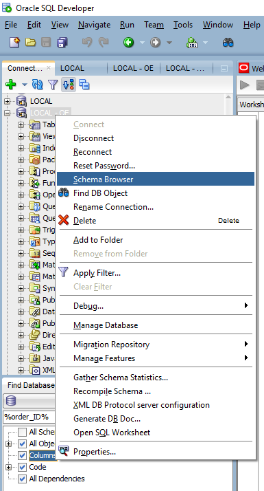
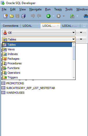
The schema browser shows Tables, Views, Indexes, Packages, Procedures, Functions, Operators, Triggers, Types, Sequences, Materialized Views, Synonyms, and few other object types for the selected schema.

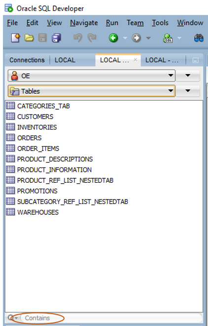
One other option is to search the objects by name in the selected type. To do this, type the search string in the contains area.

 

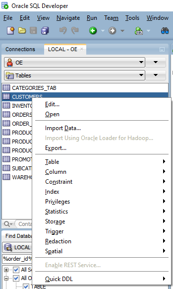
From here, based on the object type, all its related operations can be performed at ease. By right-clicking on the object, it can be viewed, edited, recompiled, or executed. The below figure shows the whole range of operations available for table oe.customers.

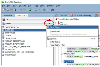
By clicking the down arrow next to Tables, New Table can be created by just filling in the values without writing the DDL statement.

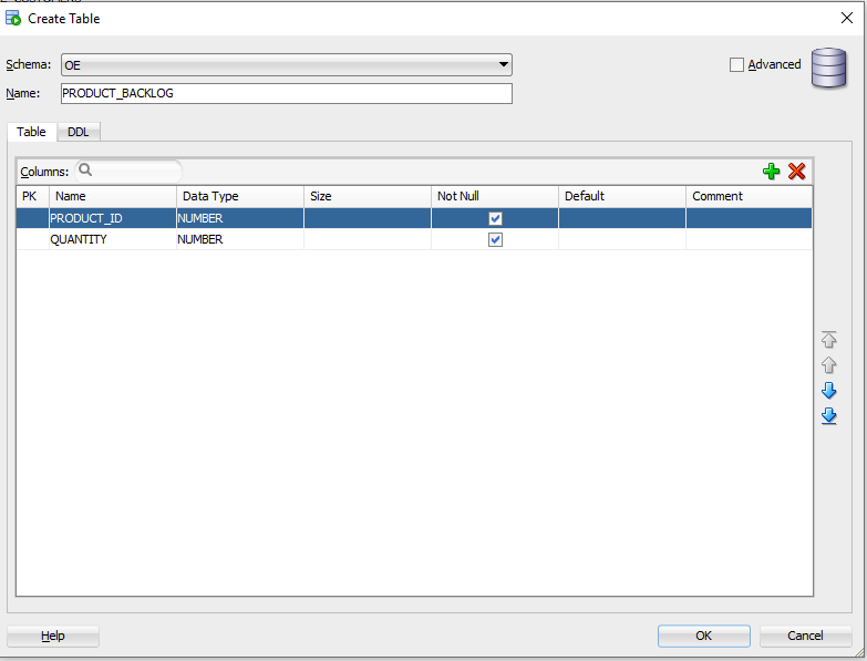
You can enter the table name, column name, data type, and all other parameters here.

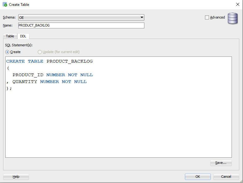
After keying in the values, the DDL tab provides the corresponding SQL statement to prepare any deployment scripts.

 

Unshared SQL worksheet and SQL History – A multi-tasker with a good memory

SQL worksheets are commonly used to run queries and to execute any PL SQL process. By default, the sheets open in shared mode. When running SQL statements in multiple sheets, the SQL statements run based on the execution order. A process run in one worksheet has to be completed for the next one to kick off.

One unique feature available in SQL Developer is to open up SQL worksheets in unshared mode. Click the Unshared SQL Worksheet icon or use the shortcut is CTRL + SHIFT + N. to open it.

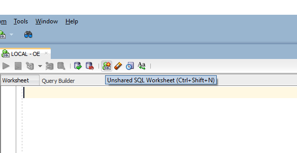
Unshared SQL worksheet helps to execute different queries or processes in parallel. Each of these sheets acts as a separate database connection. This will save a considerable amount of development time as multiple tasks can be done in parallel, like fetching data from two different views, validating more than one process, etc. The unshared SQL worksheets contain a * icon in the sheet name.

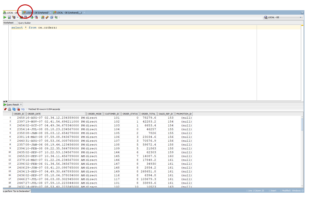
These unshared SQL worksheets work as independent sessions, and so a DML operation performed on one worksheet does not reflect on the other until it is committed. The update statement executed in sheet LOCAL – OE (Unshared) does not reflect in the data used in other worksheets without running a commit.

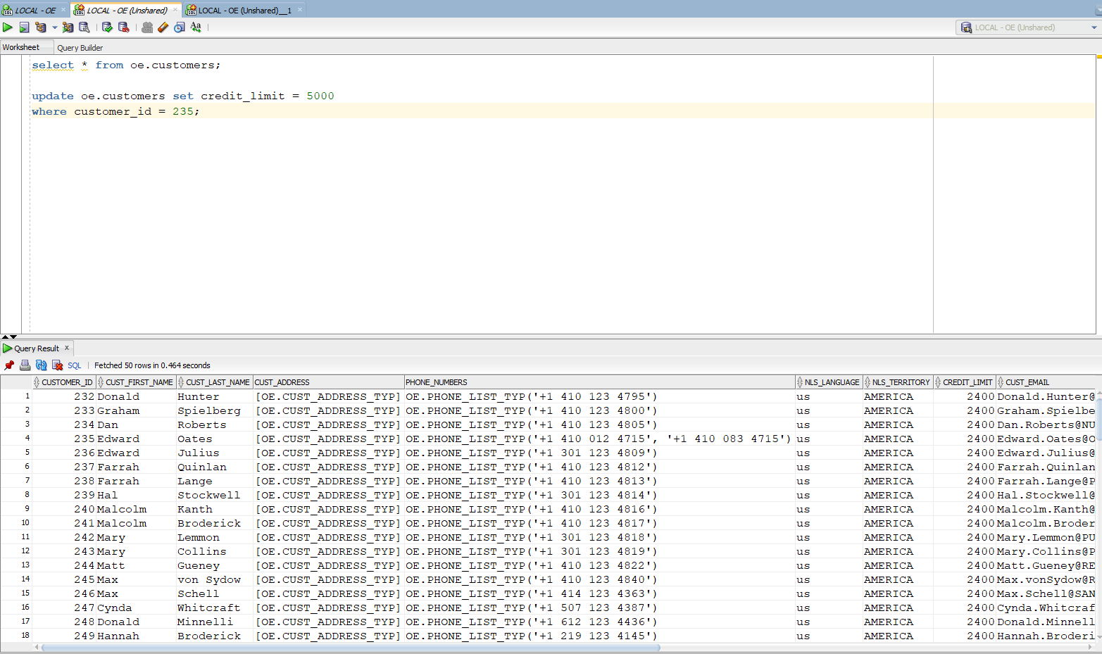
Also, any number of repeated rollbacks can be performed without impacting data on other sessions. This provides the flexibility of handling data in two or more ways simultaneously for any specific testing. Multiple unshared SQL worksheets can be opened up from each database connection.

If the sessions disconnect for any reason, the tool automatically reconnects when a SQL is executed in this sheet. A good practice would be to limit the number of unshared worksheets to two or three, as it would be hard to keep track of what operations are performed in each of the sheets.

The SQL history option would be your savior if you forgot to store your recently executed SQL statements or PL SQL process. Go to Tools -> Preferences -> Environment -> Local history to enable history or modify settings, and by default, this option will be enabled.

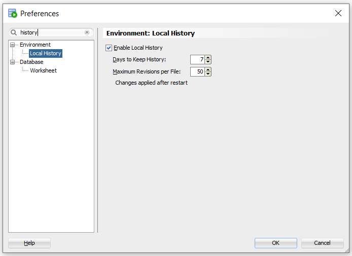
This saves the history of executed SQL statements in the current SQL Developer session. With this, you can pull most of the recently executed SQL with a single click. It is also helpful when you keep enhancing a SQL statement and later refer back to its previous versions.

To open up the history, hit the F8 key or right-click and choose SQL history on any SQL worksheet.

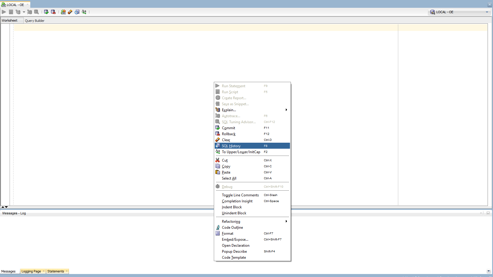
The SQL history opens up at the bottom and now, choose the required SQL statements. Click the to append the selected statements to the existing SQL worksheet. You can highlight multiple SQL statements and copy all of them to the worksheet at once.

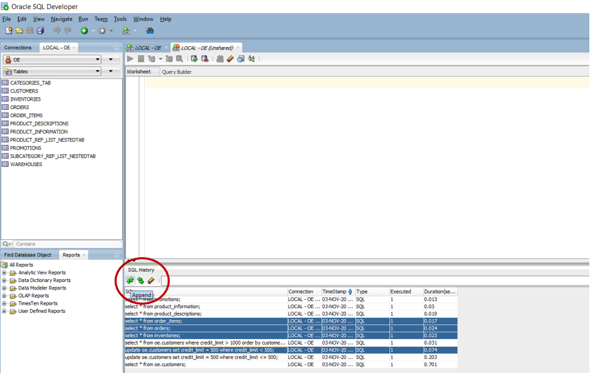
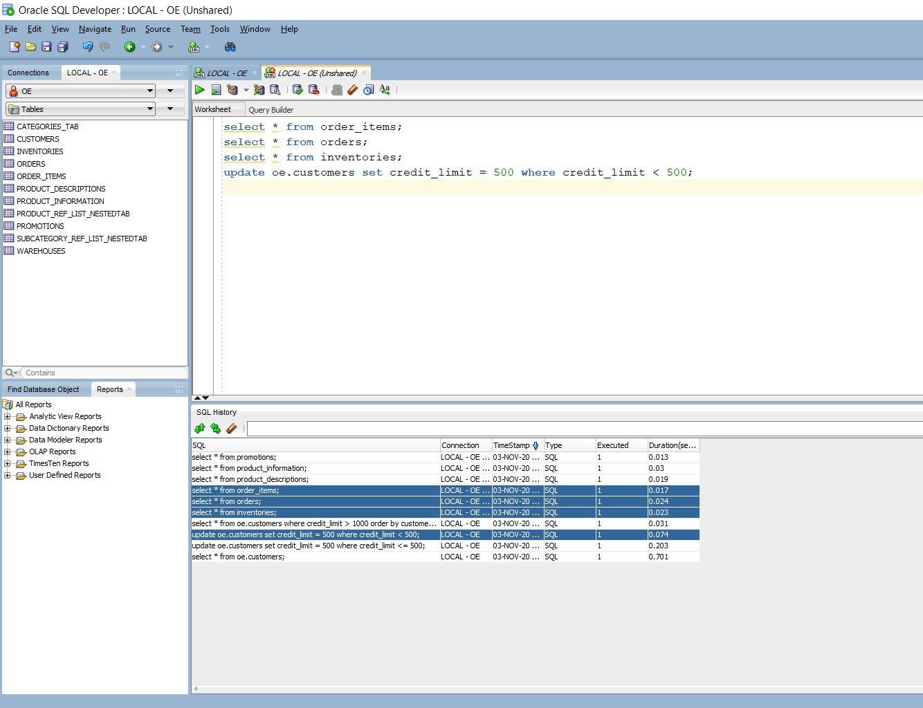
The highlighted SQL statements got added to the SQL worksheet in one shot.

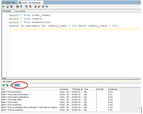
There is also a search option with this window. This helps to narrow down the SQL statements based on an object name, SQL functions used, or any other specific detail from the SQL statement. The keyword select is entered in the search box to filter only SQL statements containing select.

Find DB object – Catch me if you can

This search feature is great to perform impact analysis across the database. It helps to identify the dependencies and directly look into the code segment containing the object name or literals or any other search string. Go to View -> Find DB object to open up the window.

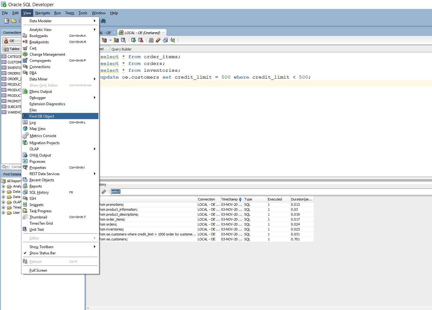
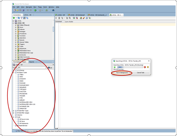
You can customize the search by selecting the required schemas, object types, or include/exclude source code. If a search is going to take a long time, it can be run in the background as well; this allows you to work on other items when the search is running.

The various objects using the searched string are shown.

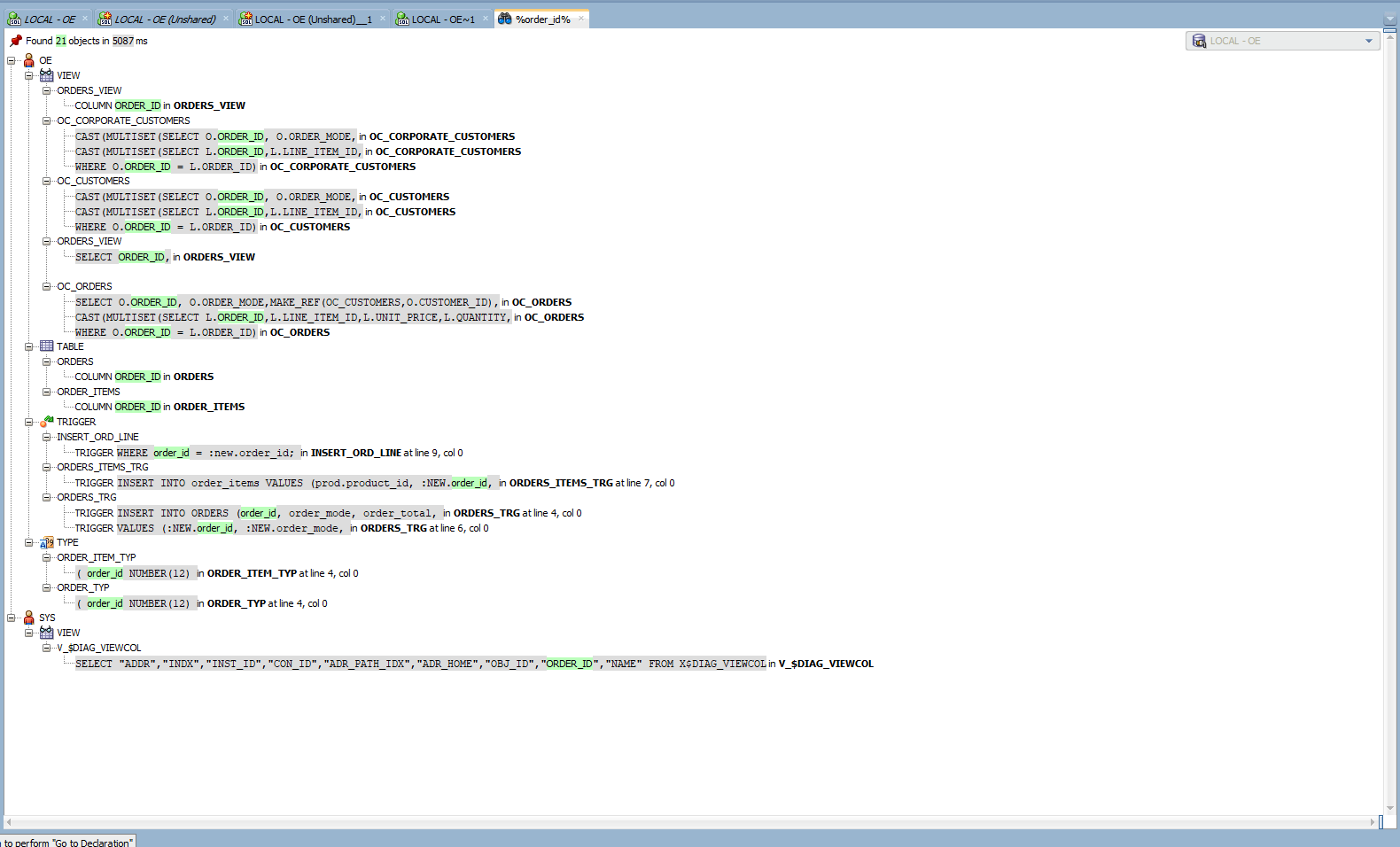
By clicking the line of code from the search results, the respective object opens up. With this, you can quickly look into all the impacted objects and save many clicks in individually opening them through a schema browser.

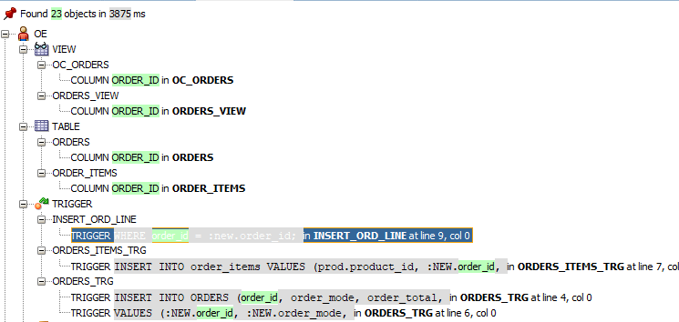
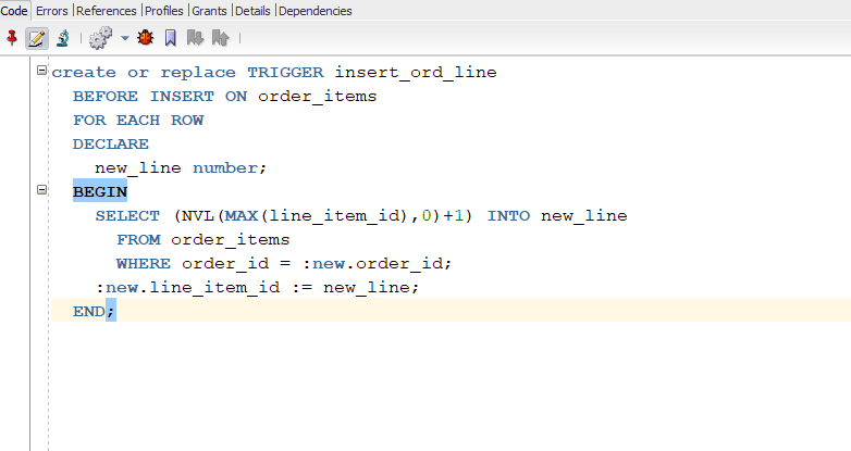
The trigger INSERT_ORD_LINE opens up after clicking it from the search results, as shown below.

Search results can also be collapsed or expanded at the schema level.

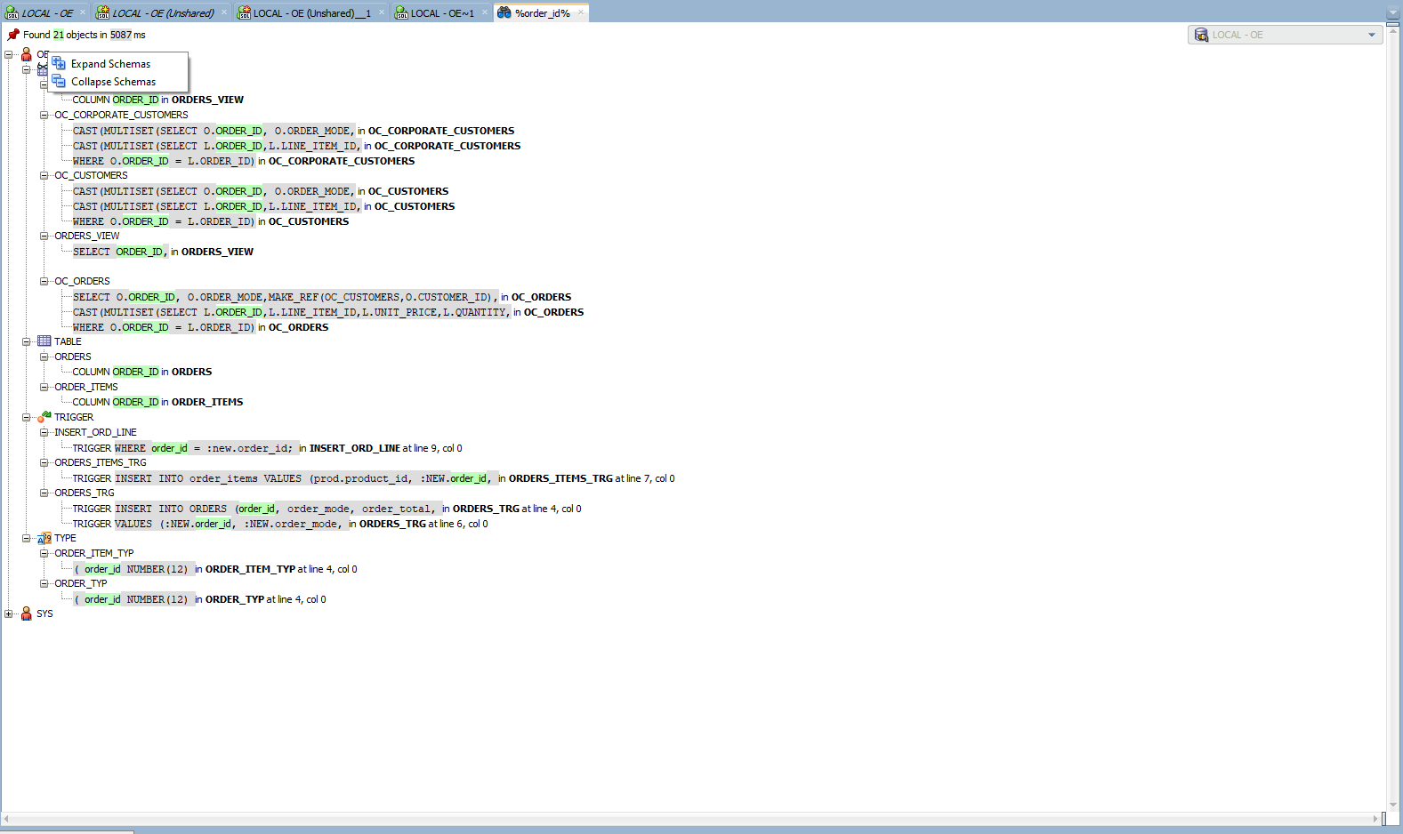
There is a limitation in the output; only up to 500 records are displayed on this search screen. For any extensive searches, one approach would be to break it down into multiple searches restricting into limited schemas.

Database compare – Catch the difference

This option helps to compare two schemas, usually between different databases. Navigate to Tools -> Database Diff to access it. After refreshing the database or post-deployment, you can run this process to ensure the required objects are available or to check if the migration is successful.

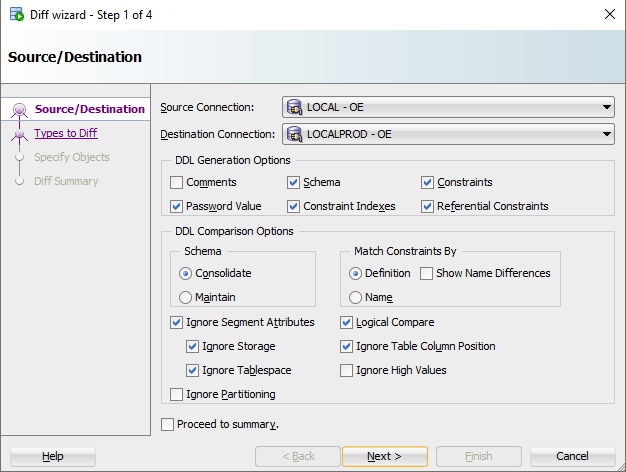
After clicking Database Diff, choose the database connections and various other comparison options in Step 1 of 4.

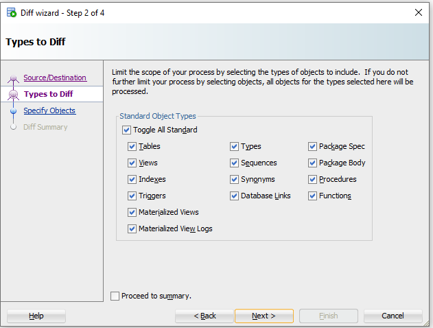
Choose the object types to be compared between the selected schemas in Step 2 of 4.

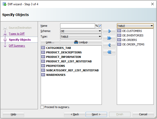
In Step 3 of 4, you have an option to run the comparison for a specific set of objects. To do that, select the schema, type, and click . The list of all items is shown; choose the required ones, click to finalize. To include all objects, just hit Next and move on.

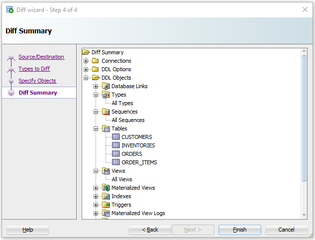
In Step 4 of 4, the summary of the comparison performed is shown. Click Finish to generate the report. As you can see, for tables, only the identified ones from Step 3 are included.

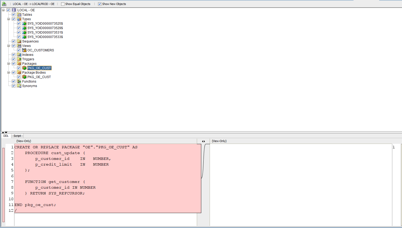
The summary of the comparison is shown below. Any objects available in one schema but not in another is highlighted in green. You can see the details by clicking the item. PKG_OE_CUST is available in the LOCAL_OE Database and not available in LOCAL_PROD database.

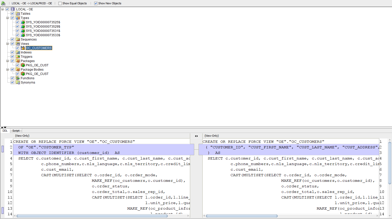
Similarly, a warning sign is used to highlight any difference in the objects between the two schemas. Click the item and view the differences.

This process also can be executed in the background to gain some productivity.

Reports – Tell me about everything

SQL Developer contains standard reports which help to quickly browse through the contents and save time compared to manually running the queries required to get those data. This option is available from View -> Reports. This will open a window listing all the available reports

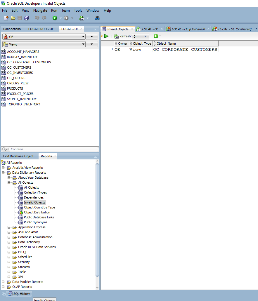
Invalid objects – This report provides a list of all invalid objects and can be run before and after deployments to ensure no new invalid objects are created.

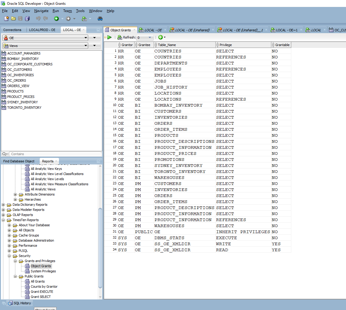
Object Grants report – This provides the overall view of grants assigned to the individual schemas.

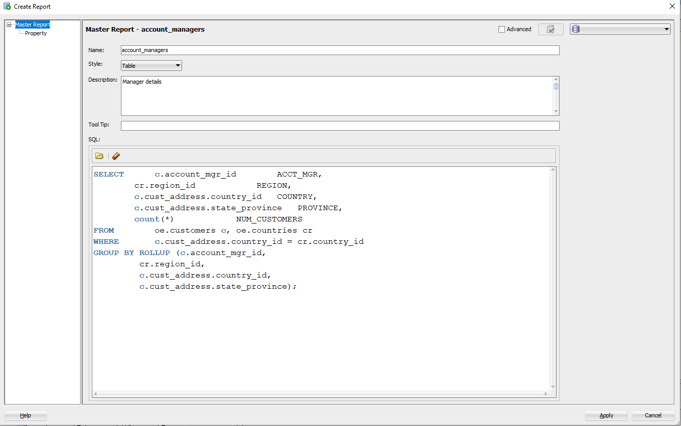
Custom reports are also available in SQL Developer under Reports -> User Defined Reports. By right-clicking on User Defined Report and choosing New report, the below screen opens up. You can save any frequently used report or SQL with a report name.

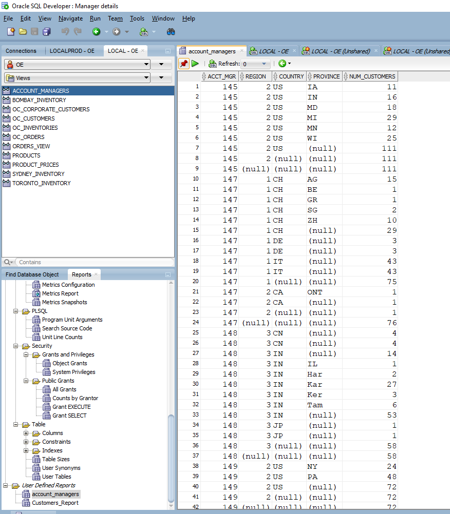
Click on the report name to view the results from the newly created report.

Pinning – Stay where you are

This is a minuscule item but saves many repeated clicks, especially if you are new to SQL Developer. When you open a new object, SQL Developer automatically closes the tab for certain object types. When I open the oe.customers table to view it and then open the oe.oc_inventories table, it closes the oe.customers window. In a way, it helps avoid accumulating a lot of tabs to browse through back and forth. But if you would like to keep the tab open, then it can be pinned.

You can pin the window with the universal icon , and it is always on the top left corner of the window. Any pinned tabs must be manually closed.

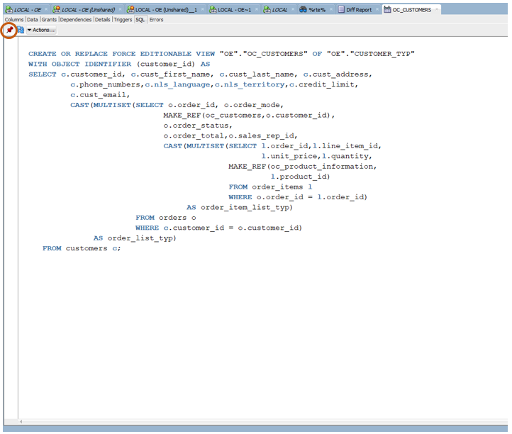
In PL SQL packages, procedures, functions, and few other object types, the windows are automatically pinned, which means opening another package does not close the existing package.

Format and Explain Plan – Make it legible

After developing a PL SQL object, the code can be formatted using the format option (ctrl + F7) or right-clicking on the SQL worksheet and choosing Format. The settings related to the format can be controlled in the preferences section (Tools -> Preferences -> Code Editor -> Format). The formatter settings can be auto-detected as well.

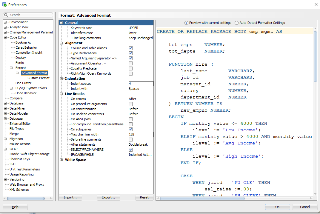
A common standard can be created across the team, which would help maintain the same code format and easier maintenance. Selected pieces of code can also be formatted by highlighting only the required portion and formatting it.

The explain plan option helps evaluate the cost and the sequence of operations performed in the SQL statement. This is available from the SQL worksheet and can be viewed by hitting the F10 key or right-clicking and choosing Explain Plan. The cost and cardinality for the SQL statement are shown.

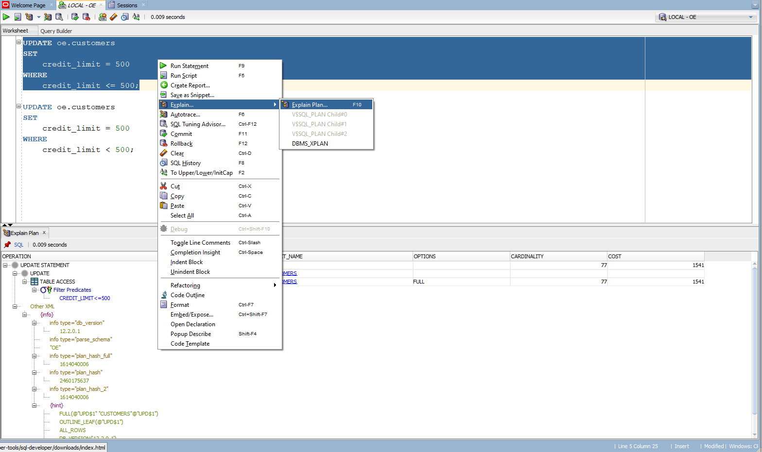
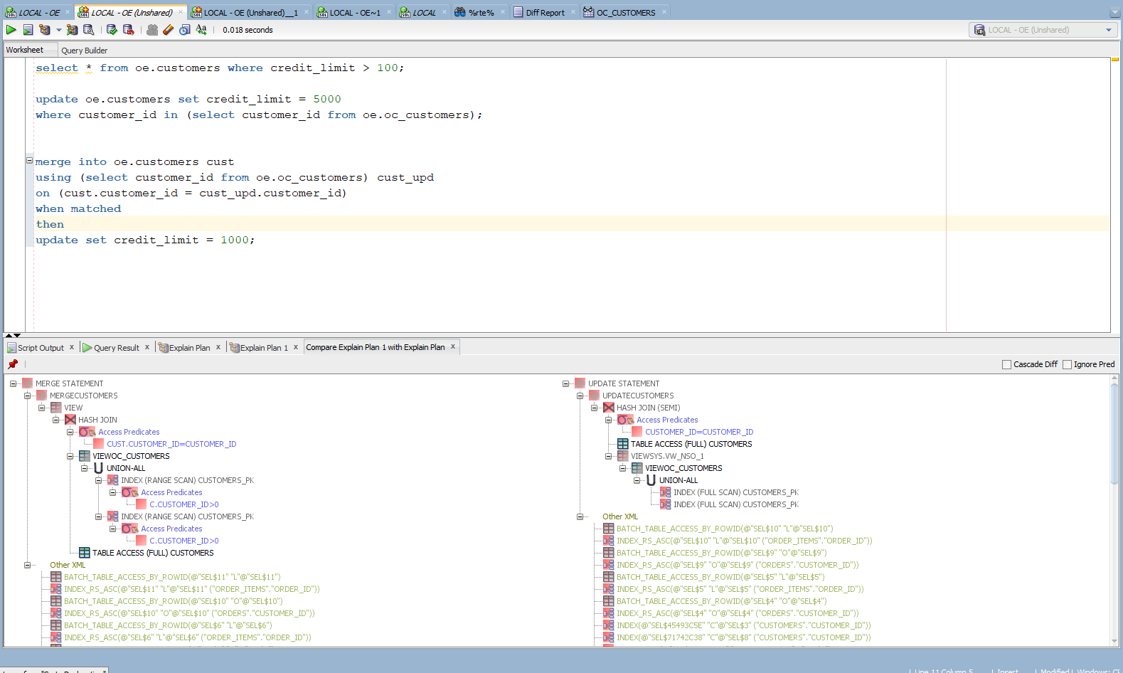
Two different explain plans can be compared to see the difference in steps. Usually, this is done when tuning queries to look for any improvements. Generate the explain plan for the first statement and remember to pin it.

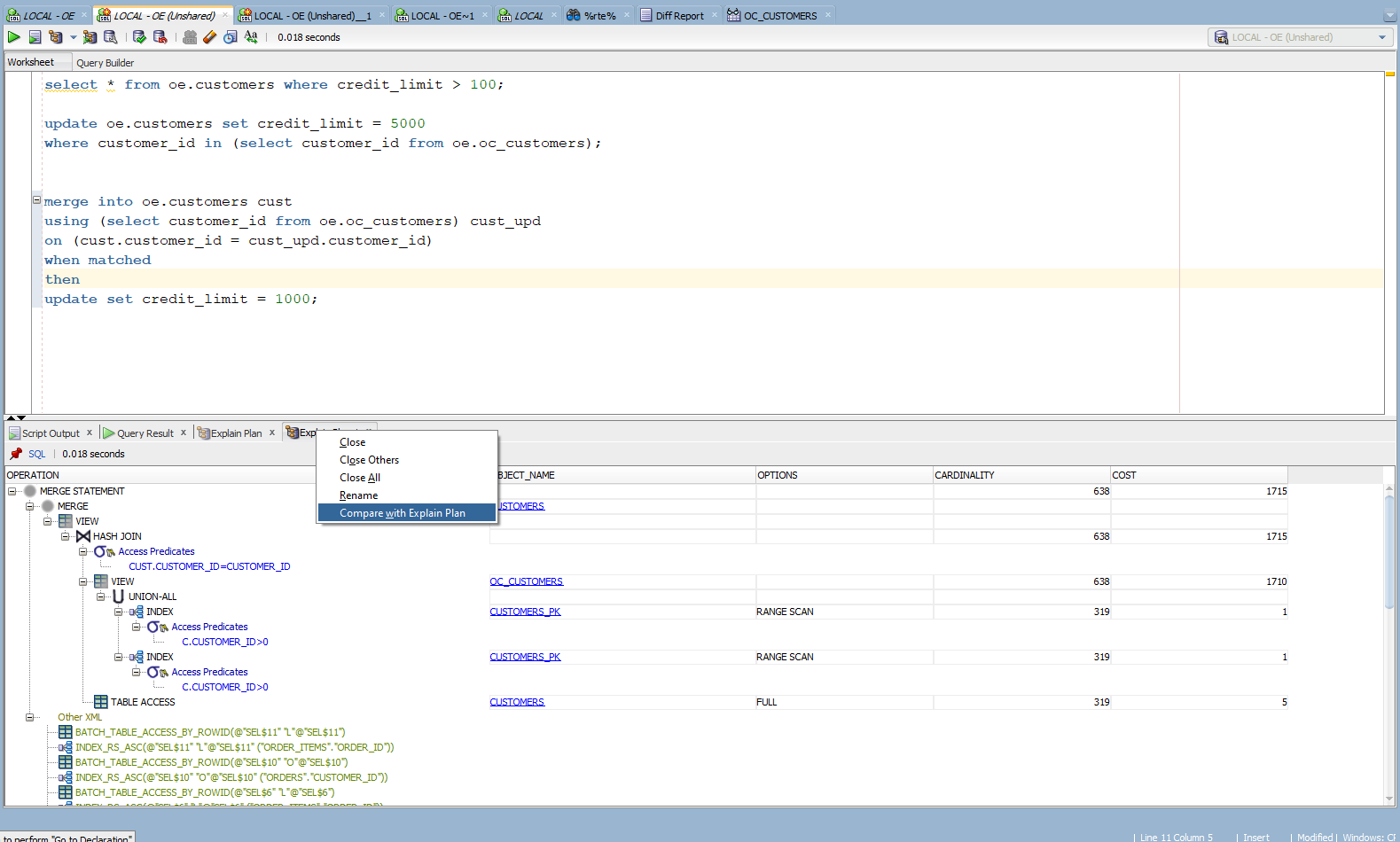
Now, generate for the next statement and right-click on the second explain plan tab to compare with the first one. This helps to compare the plans side by side.

Debugging – A blessing for every developer

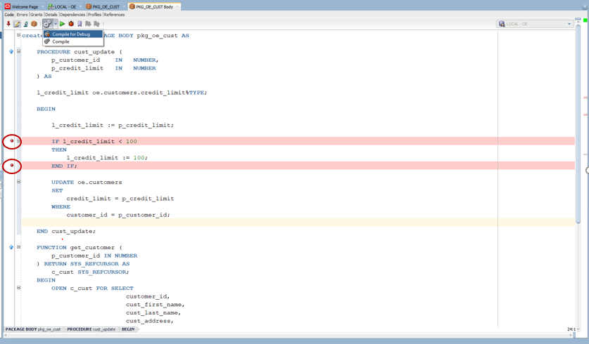
SQL Developer has a debugging feature for the PL SQL programs. A specific procedure, function, or package can be debugged with breakpoints, and the value of the variables can be observed during the execution. To set a breakpoint, click on the desired line of code on its left side and compile it with the debug option.

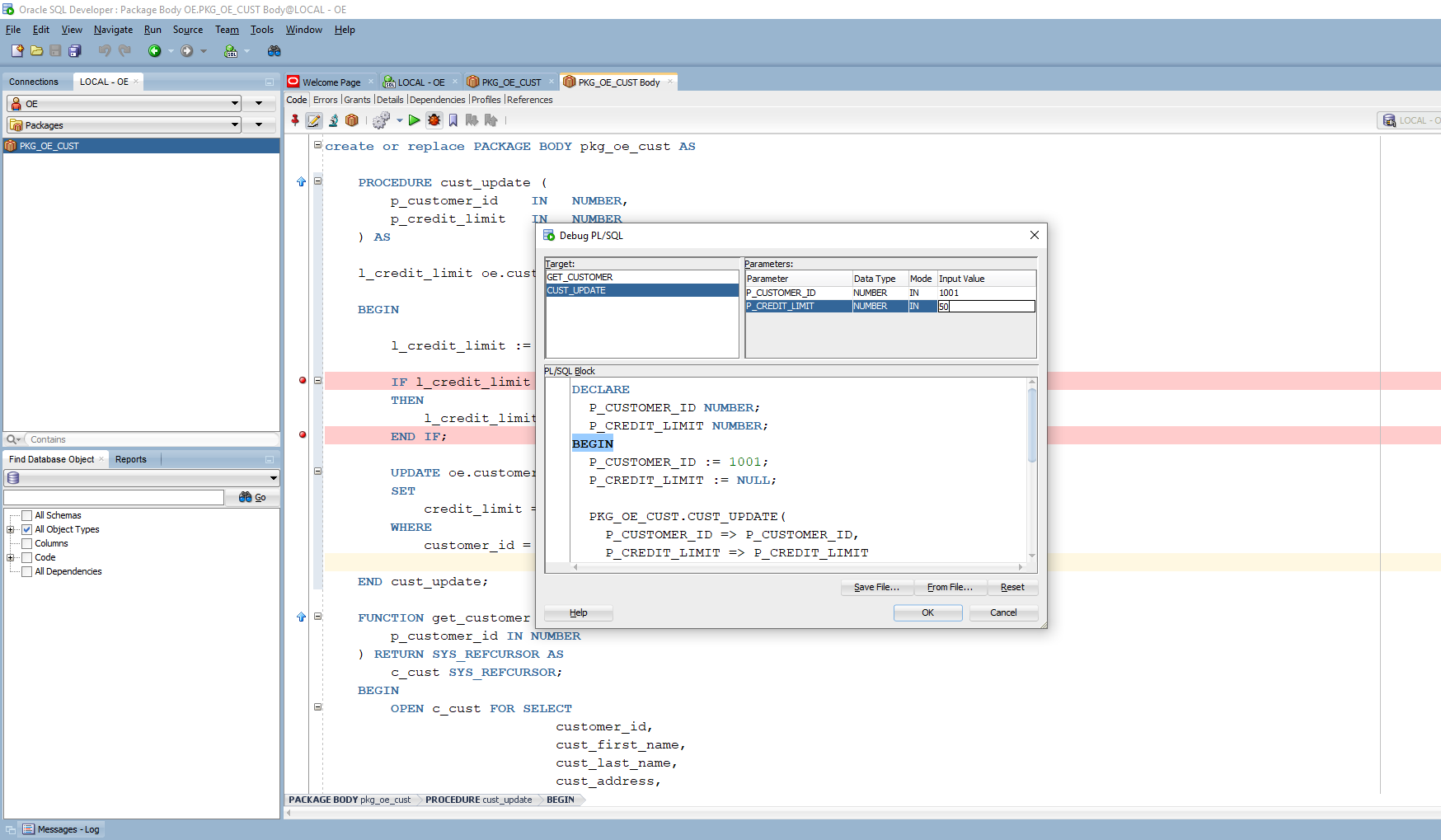
Click the icon to start the debug process. The input values to be provided during execution can be keyed in the parameters section. The program gets executed after clicking OK. I have provided an input value of 1001 to p_customer_id and 50 to p_credit_limit.

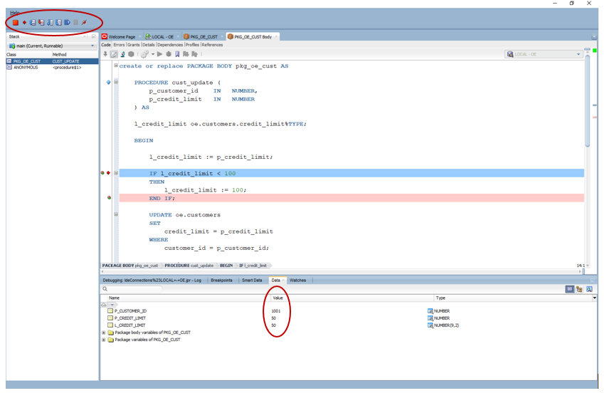
Now, the process has stopped at the breakpoint. Here, a whole range of operations can be performed. Under the Data tab, the values of the variables can be observed as the process gets executed. With the icons on the top, the debugging process can be stopped, resumed, moved into another subprogram, etc.

Under the Data tab, you can observe that l_credit_limit is set to 50 before entering the IF clause.

After hitting or F9 to resume, the process stops at the next breakpoint. Here, you can observe, the l_credit_limit value is updated to 100.

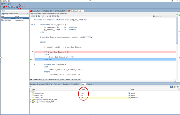
Hitting or F9 to resume will complete the execution of the cust_update procedure, as there are no more breakpoints.

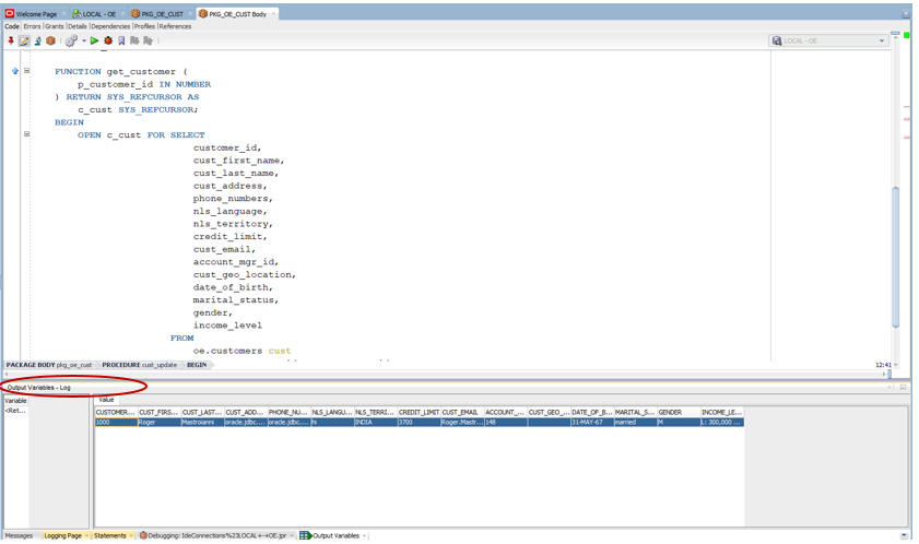
If there are output cursors returned as part of a function, the cursors’ dataset can be viewed as well. The procedure get_customers returns a cursor to view the customer details for an input customer. The process is executed by clicking , entering 1000 for p_customer_id under the parameters section, and clicking OK.

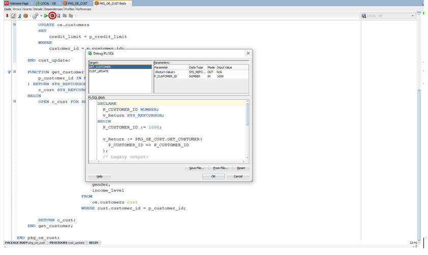
After running the function, the cursor’s output value is shown under the Output Variables – Log section.

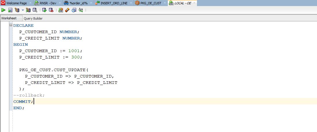
In some instances, the code block to execute the procedure or function can be copied to a SQL worksheet and executed from there. This helps to quickly set up the parameters when running these processes from a worksheet. The p_customer_id is set to 1001 and p_credit_limit to 300. This process can be executed several times for different values directly from this SQL worksheet by clicking on the top left.

Sessions monitor – What’s going on

The sessions monitor screen identifies the active sessions currently executed in the database with details like SQL Id, SID, execution time, OS user, client identifier, and many others. It can be opened up from Tools -> Monitor Sessions. If you have any long-running processes, those can be identified here and you can monitor the batch processes.

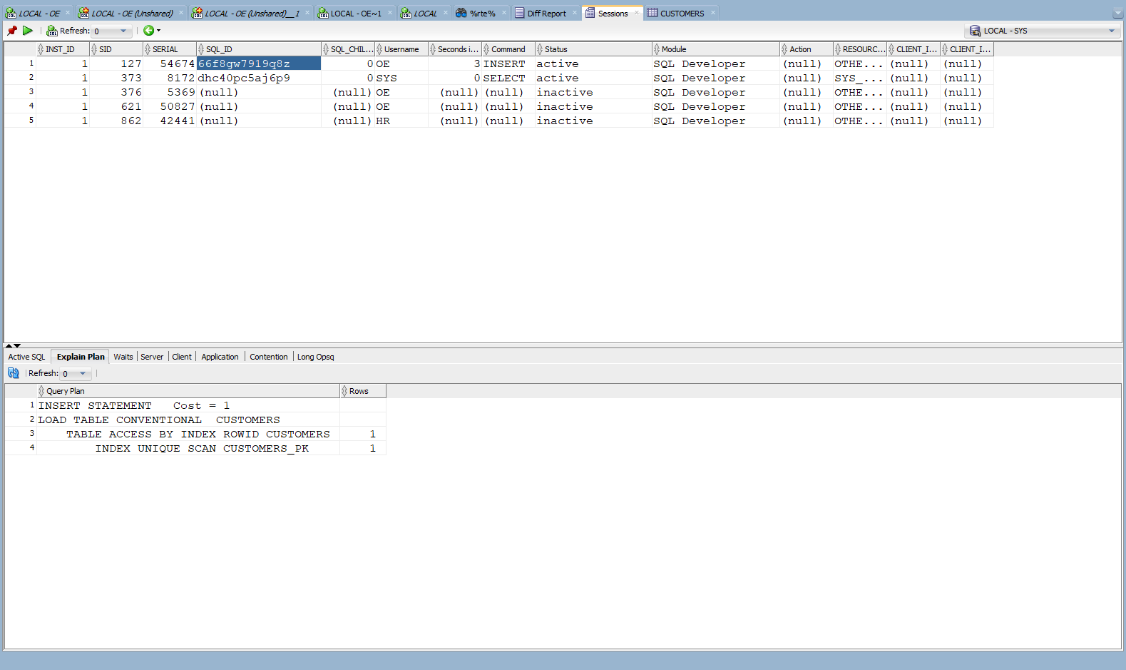
There is a refresh timer at the top, which can be set for an automatic refresh of the screen. Filters can be applied at the top of each column to look for sessions only under a particular schema, specific OS user, or only active sessions.

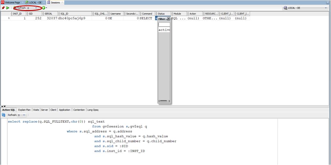
It would be hard to capture any process which takes less than a few seconds here, and a better approach would always be creating debug logs for such processes. In the case of SQL statements with bind variables, this does not show the bind values; rather only displays them as bind variables.

The wait tab at the bottom shows any session waits caused due to object locks or resource availability. The Active SQL tab displays the exact statement currently executed by the process, and the Explain Plan tab shows the cost associated with the statement and execution plan.

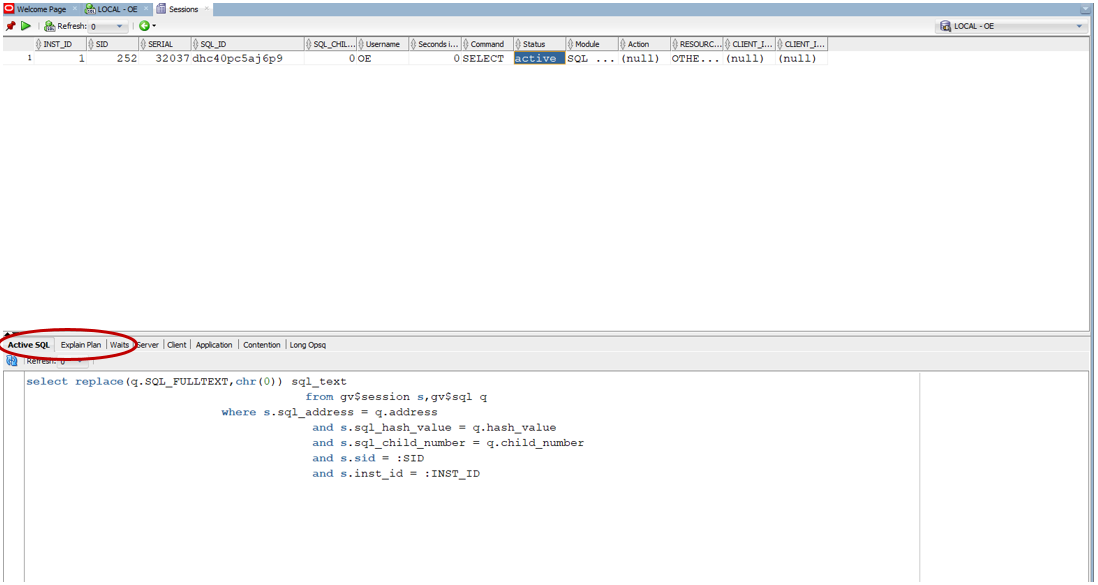
These features help to quickly get a grasp of the current processes executed in the database.

Database Design diagram – A must-have artifact

A data model diagram of the database assists in understanding the relationships between the objects. The option is available under File -> Data Modeler -> Import -> Data Dictionary. After choosing the connection to log in, the list of schemas can be selected.

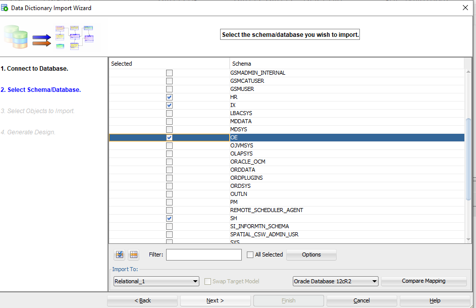
Following that would be a screen to select tables, views, and any other objects. After choosing those, hit finish. To select all the tables, use the check all icon at the bottom left.

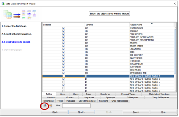
The data model diagram showing the relationships between the objects and keys, indices, and many other details is provided. These details are entirely customizable, and the diagram can be saved as a PDF or Image file by right-clicking and choosing Print Diagram -> To image file / To PDF file.

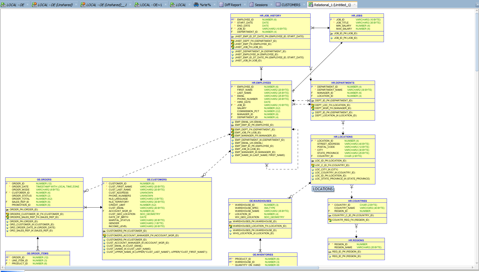
This is one of the essential artifacts maintained for the database, and it also helps to perform the impact analysis at a high level.

Get the most from SQL Developer

Just like any other tool, you get used to this and discovery new functionality as you start working in it. The tool is easy to set it up and does not require the Oracle client to be installed. There are a lot more features and utilities available in this tool apart from the items discussed here. Give SQL Developer a try and improve your skills.

Use the links below to download the SQL Developer and the documentation to explore further.

https://www.oracle.com/tools/downloads/sqldev-downloads.html

https://docs.oracle.com/en/database/oracle/sql-developer/20.2/books.html

 

The post SQL Developer – A great tool and better ways to use it appeared first on Simple Talk.

from Simple Talk https://ift.tt/3nG4Sti
via

Database DevOps Considerations for SQL Server Availability Groups

One question which comes up periodically from our Microsoft Data Platform customers is whether there is anything special that they need to do when implementing version control, continuous integration, and automated deployments for a production database which is a member of a SQL Server Availability Group. 

The good news is that deployments are quite straightforward. You’ve most likely already configured a listener for your applications to connect to the Availability Group and automatically find the writeable database. To do a deployment, you simply need to connect to the listener as well.

There are a few other considerations which are helpful to think about when building your approach to database DevOps, however.

A migrations approach gives you needed flexibility for Availability Groups

Managing Availability Groups can be quite tricky. This is especially true if you have large databases, or if you sometimes experience latency to some of your secondary databases.

For example, operations like creating an index may generate a large amount of log data which needs to be transferred to your secondaries. If you need to do this in a deployment, you may wish to customize the deployment by adding a command to wait for a period of time after doing the operation. 

A ‘migrations’ approach to database deployment — for example what we have in Redgate Deploy’s SQL Change Automation, which automatically generates code for you at the time of development — gives you the ability to easily customize your deployment scripts in any way you like. You might even choose to write a  wait for statement which uses SQL Server’s dynamic management views to check log queue sizes for your secondaries and act accordingly. 

As a contrast, with a ‘state’ based approach to database deployment — for example what we have in SQL Source Control — schema changes are automatically generated by an automated comparison process at the time of deployment. While this is convenient, it doesn’t have the flexibility which is helpful for more complex environments such as Availability Groups. With this approach, you will likely want to isolate longer running commands into their own deployments.

SQL Agent jobs need special handling

If you have SQL Agent jobs related to your database, you can add these into source control if you wish. 

SQL Agent jobs are a bit special, as the code for these jobs doesn’t reside in user databases. Instead, the code for all the jobs resides in the msdb system database. 

In an Availability Group scenario, typically there is a desire to have SQL Server Agent Jobs configured on all members of the Availability Group, and to use conditional logic within the job to determine if the job should run or not.

If this is the case for you, it probably means that you want to deploy code for your jobs to all nodes in the Availability Group cluster — not only to a single “writeable” primary database.

I think the easiest way to manage this is to create and version control a user database for administrative purposes, perhaps named Admin or DBA. This database and repository can contain code for both instance level objects (SQL Agent Jobs, Linked Servers, etc.) as well as other helpful objects that you may use for administration on the instance, such as the free community sp_WhoIsActive procedure.

If you are using the ‘state’ based approach (SQL Source Control or a similar solution), you will need to store the code for instance-level objects in a post-deployment script, as the code needs to run in another database. This is an optional choice with the migrations-based approach of SQL Change Automation, but it is convenient there as well.

Consider having a staging environment with Availability Groups in your pipeline

In my experience, Availability Groups are complex enough that it makes sense to have a staging environment for them. This means having full-sized production like datasets, configured in the same AG topology that you have in production. 

This is valuable as it can help you identify changes which make take a long time to execute and/or generate significant amounts of log. 

This also means that you don’t necessarily have to configure all your development environments as Availability Groups. Because most features of AGs tend to be transparent, I’ve found that having AGs in all environments hampers development more than helps it.

 

 

The post Database DevOps Considerations for SQL Server Availability Groups appeared first on Simple Talk.

from Simple Talk https://ift.tt/36I2KdC
via

Three ways that taking the State of Database DevOps Survey helps the community

Redgate has recently opened the 2021 State of Database DevOps Survey.

Whether or not your organization does DevOps, I would love for you to take the survey. The survey will require around 15 minutes of your time, but I think it’s a great investment as it will benefit the whole community of database administrators, developers, and leaders in IT and development.

Here’s how it helps:

1. The survey helps you and others drive change in your organizations
I hear from loads of DBAs and developers that they have a hard time making a case to modernize their infrastructure and processes. Research like the State of Database DevOps report is a major help to data professionals in this area: when making a business case, this research gives you real-world insights and data to reference. The survey is not specific to any specific database platform or vendor (including Redgate), so the Report and findings can be useful to you no matter what tech stack you are using.

2. The survey helps everyone understand how IT is shifting for databases
Redgate has been running the State of Database DevOps survey for years, which allows us to see insights in how the software development lifecycle is shifting for databases.

While there are other surveys on IT and DevOps, this is largest, longest running survey on databases. This means that the survey can uniquely help the community understand how database development and operations are changing over time.

3. Redgate gives back for each survey response
For each submission we receive for the survey, Redgate will donate $1 to the World Health Organizations COVID-19 Solidarity Response Fund. And there could be something for you directly too — you have the option to enter and win a $500 Amazon Voucher, should you like.

I hope that you’ll take the survey today, and also share it with your colleagues.

The post Three ways that taking the State of Database DevOps Survey helps the community appeared first on Simple Talk.

from Simple Talk https://ift.tt/36D0TXC
via

DBA in training: Backups, SLAs, and restore strategies

The series so far:

1. DBA in training: So, you want to be a DBA...
2. DBA in training: Preparing for interviews
3. DBA in training: Know your environment(s)
4. DBA in training: Security
5. DBA in training: Backups, SLAs, and restore strategies

A DBA’s job is getting the right data to the right people as quickly as possible.

Consider that first part – getting the right data. How do you do that? By having the data in the first place. The best way to ensure that you have the data is to look at your company’s needs, recommend availability options, and most importantly, do backups. Few things will get a DBA fired more quickly than not having backups available when they are needed. It may be years before you ever have to restore a database from a backup, but the backups had better be there when you need to do one.

Conference sessions and books have been written on the subjects of backup/restores, SLAs, and availability options, and they are so good that I’ll just give you a brief overview here. You’ll gravitate to your need-to-learns soon enough.

As soon as you have a list of the SQL Server instances you will be managing, you need to understand three acronyms thoroughly:

• SLA
• RPO
• RTO

Did you just read those sets of three letters and wonder what I’m talking about? Don’t worry; I will explain.

Service Level Agreements (SLA)

Service Level Agreements (SLA) are a set of agreements between you and the business. Among other points (which may vary by the organization), they cover RPOs and RTOs.

Recovery Point Objective (RPO)

RPO is broadly defined as “how much data can you afford to lose if the data has to be recovered”.

Recovery Time Objective (RTO)

If RPO is a measure of how much data can be lost, RTO is a measure of how much time the business can afford to be down if data recovery becomes necessary. In other words, how long until you are back online and ready to go?

Ask to read over the SLA – in particular, the RPO and RTO. If there isn’t one, then find out what would need to be done to put one in place. Then, determine whether anyone has ever tested the numbers to ensure that they are possible.

Finally, try doing some tests yourself (not on Production!). In particular, try implementing some database restore strategies in test and see how long they take. If the numbers in the SLA appear too low or inconsistent with what your tests are showing, now is the time to note that and to consider alternatives to recommend. There are high availability options that can greatly improve your downtime if your instances are on-premises, and if your company uses a cloud option, RPO and RTO are configurable there as well. However, your restores are another matter. If your restores are taking too long no matter what you do, or you think the numbers in the SLA are unachievable for some other reason, your test results might help to facilitate the discussion of what revisions need to be made to the agreement, and what the costs of those changes will be for the company.

Backup and Restore Strategies

You may use options to increase the availability of your databases, but it would be a mistake to assume that having an availability strategy by itself guarantees the safety of your company’s data. You may, for instance, have Always On availability groups. These are groups of one or more databases that are copied out to at least one other location. If something would happen to the primary instance, the database administrator has the option to either manually or automatically “failover” to the other location with a minimum of downtime. Availability groups can have issues or fail outright. Worse, you may find yourself in a situation where a data entry mistake occurs. Maybe someone did a data update (or worse, a delete) with an incorrect or absent WHERE clause, for instance. That is when the phone starts ringing, and the incidents come in.

What, you have no backups? Houston, we have a problem. The best availability insurance you can provide for your company is to have tested, proven backups, and a layered practiced restore strategy.

Okay, you may think. I know I need to take backups, no matter what, but how do I test and prove them? Why do I need to practice restoring them?

The answer is simple: Because things go wrong with backups, too, and if you haven’t even tested them, you could be putting your business at risk of data loss. Make sure to do everything possible to ensure that doesn’t happen to you. I will start from the beginning by talking about recovery models and backup/restore strategies.

Recovery Models

Whenever you are asked to create a new database (or if one is created during a deployment) one of your first questions should be centered around what recovery model the data owner needs. Here are your options:

FULL recovery

This is used for point-in-time restores – for example, a business user might request that you restore the database to a week ago at 7:15 in the morning. Point-in-time restores allow you to restore your database to any point in time, rather than just the time the backup was taken. If your data changes frequently, this is probably the option you need.

With FULL recovery, everything that happens on the database is recorded to the transaction log. That means that the log now has enough detail to go back to a moment in time and put the data to the exact state it was then – which affords you that point-in-time flexibility. It is important to understand that though you may take a full backup, your transaction log won’t be cleared until you do a log backup. If you forget to set up transaction log backups on this recovery model, the transaction log will balloon like a kinked water hose until eventually, it brings database activity to a screaming halt.

BULK-LOGGED recovery

You would use this primarily when you are loading a good amount of data into some tables. The load will be minimally logged, affording it speed and efficiency, but losing the detailed playback mechanism that makes point-in-time possible.

Not every operation qualifies for minimal logging. Some operations that do are:

• Bulk INSERT and SELECT
• SELECT INTO
• Creating indexes
• TRUNCATING tables
• Partition switching

The BULK-LOGGED recovery model is intended for temporary situations. However, there is a catch with point-in-time restores. The point-in-time capability is lost for any transaction log backups that contain bulk operations, along with tail log backups. Once the bulk operation is complete, switch the recovery model back and perform a FULL backup to start another chain.

SIMPLE recovery 

Use this if you don’t need point-in-time recovery, because you won’t be able to do log backups with this. This is a great recovery model if your data changes infrequently. The transaction log will checkpoint periodically, which means that it writes any dirty pages and log records to disk. This prevents the log from becoming bloated.

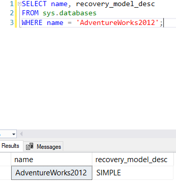
How do you figure out your recovery model? There are a couple of easy ways. The first is just to use TSQL:

SELECT name, recovery_model_desc
FROM sys.databases
WHERE name = 'AdventureWork2012';

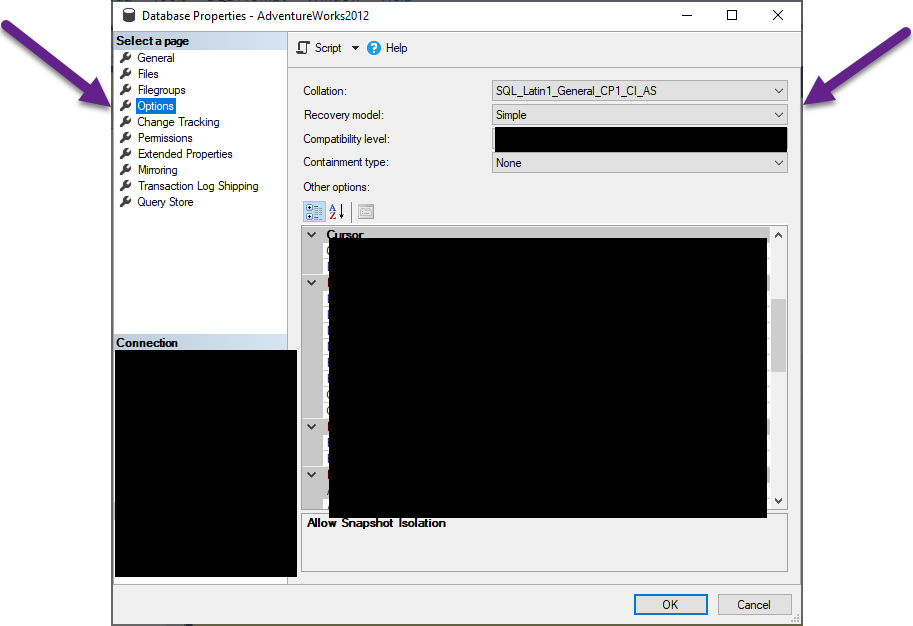
You could also just right-click on the database in the question and go to the Options window:

Backup Strategies

Once you have determined your recovery model, you can begin to think about backup strategies. How do you formulate a backup strategy? You think about how it is going to meet your RPO and RTO numbers. There are a number of ways to do this, but one of the most common starting points is to choose a combination of backup types and practice some restores to see if it is going to meet your goals.

What do I mean? When you are starting to look at backup strategies, begin with these options:

FULL backups

A FULL backup does just that – it backs up the database. It is your first step for all things backup-related, as it establishes the backup chain. In other words, the other backup types I am going to tell you about are tied to this one. You will use FULL backups no matter what the recovery model is. How frequently you use FULL backups will depend on the size of the database and your restore strategy. Most of the databases that I have worked with have received a FULL backup daily, but they could be once every few days, or even once a week.

You may find that when you start at a company, you have backup software such as Redgate’s SQL Backup or SQL Agent jobs already in place to manage your backups. You, however, should know how to do backups yourself. To do a FULL backup, I’ll pretend to do a backup of the AdventureWorks2012 database.

Using TSQL:

BACKUP DATABASE [AdventureWorks2012] 
TO  DISK = N'<location\filename here>'
WITH NOFORMAT,
                INIT,
                NAME = N'AdventureWorks2012-Full Database Backup',
                SKIP,
                NOREWIND,
                NOUNLOAD,
                COMPRESSION,
                STATS = 10,
                CHECKSUM;
GO
DECLARE @backupSetId AS INT;
SELECT @backupSetId = position
FROM msdb..backupset
WHERE database_name = N'AdventureWorks2012'
                AND backup_set_id =
                (
                        SELECT MAX(backup_set_id)
                        FROM msdb..backupset
                        WHERE database_name = N'AdventureWorks2012'
                );
IF @backupSetId IS NULL
BEGIN
RAISERROR(N'Verify failed. Backup information for database ''AdventureWorks2012'' not found.', 16, 1);
END;
RESTORE VERIFYONLY
FROM DISK = N'<location\filename here>'
WITH FILE = @backupSetId,
                NOUNLOAD,
                NOREWIND;
GO

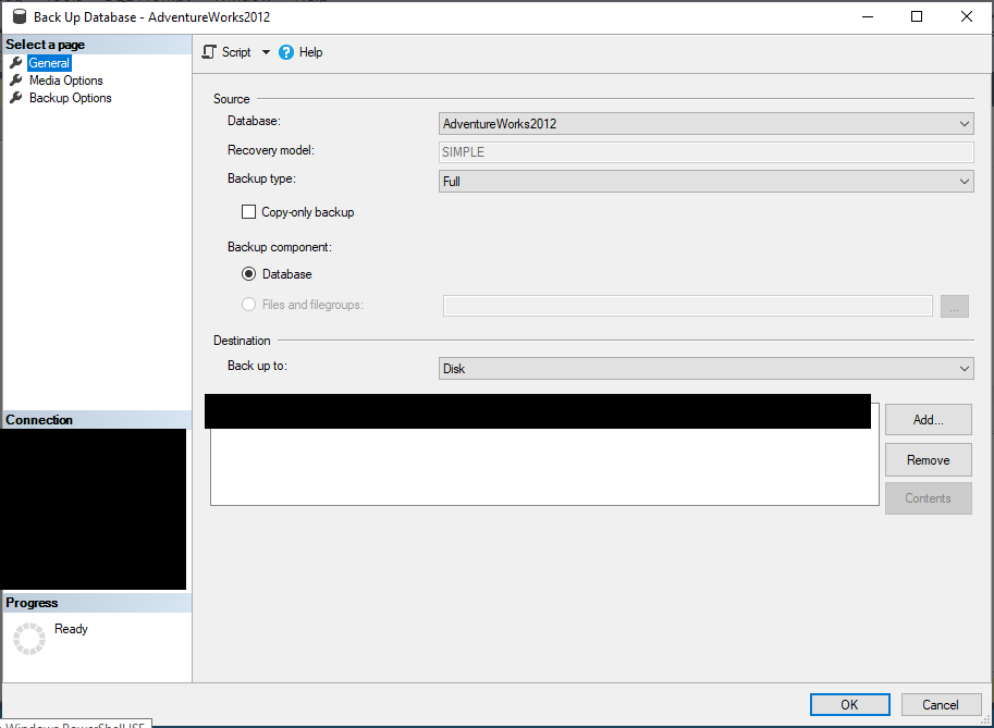
To do a FULL backup using the GUI (right-click the database, go to Tasks, then Select Backup…). Then match your screen to this on the General tab:

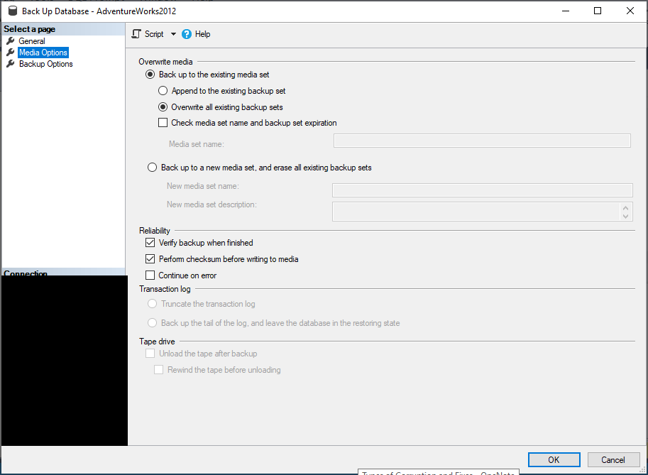
Fill in media options here:

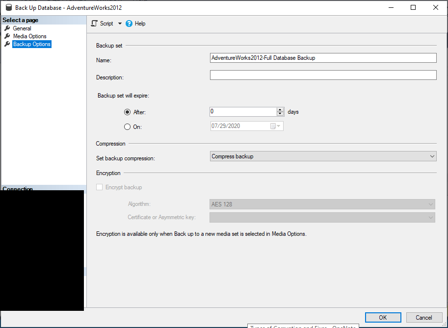
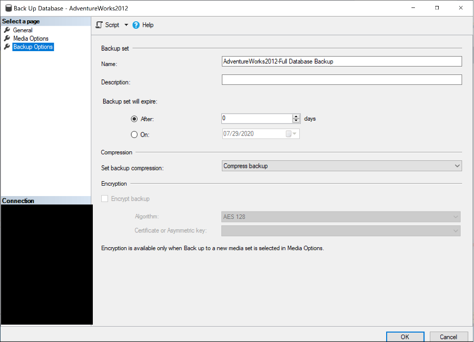
Fill in backup properties here:

There is a special option with FULLs called WITH COPY_ONLY that allows you to take a FULL backup without breaking your existing backup chain.

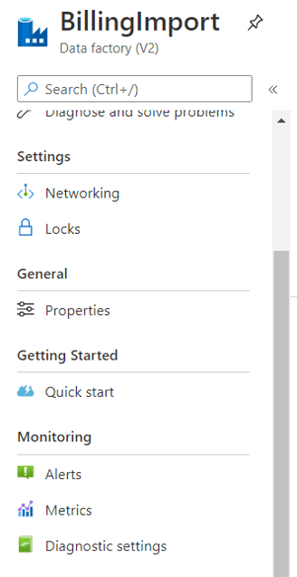
To do the COPY_ONLY backup, just add that option after the WITH clause (when using TSQL) or check the Copy-only backup box on the General window of the GUI.

DIFFERENTIAL backups

The differential backup (or “diff”) is an optional (but useful) part of the backup chain. It covers all the changes since the last full backup. These restores from these backups tend to be much faster than restores from FULL backups, so taking diffs can save you some restore time. Because it covers all the changes since the last full, it can give you some extra flexibility – although not point-in-time recoverability – and it will be important for your business users to understand that.

How many diffs do you do? The company you work for probably has an established backup schedule which includes how many differential backups it does a day per server, so you won’t need to customize to an individual database. If you find that there is no automated backup strategy and it falls to you to determine to set the schedule, start with diffs every six hours and see where that gets you with your practice restores. If you find that differential backups aren’t being done, suggest them! Differential backups lend efficiency, flexibility, and speed to your backup and restore strategies.

To do a differential backup:

Using TSQL:

BACKUP DATABASE [AdventureWorks2012]
TO  DISK = N'<filename, backup name here>'
WITH DIFFERENTIAL,
        NOFORMAT,
        INIT,
        NAME = N'AdventureWorks2012-Differential Database Backup',
        SKIP,
        NOREWIND,
        NOUNLOAD,
        COMPRESSION,
        STATS = 10,
        CHECKSUM;
GO
DECLARE @backupSetId AS INT;
SELECT @backupSetId = position
FROM msdb..backupset
WHERE database_name = N'AdventureWorks2012'
        AND backup_set_id =
                (
                        SELECT MAX(backup_set_id)
                        FROM msdb..backupset
                        WHERE database_name = N'AdventureWorks2012'
                );
IF @backupSetId IS NULL
BEGIN
RAISERROR(N'Verify failed. Backup information for database ''AdventureWorks2012'' not found.', 16, 1);
END;
RESTORE VERIFYONLY
FROM DISK = N'<filename, backup name here>'
WITH FILE = @backupSetId,
        NOUNLOAD,
        NOREWIND;
GO

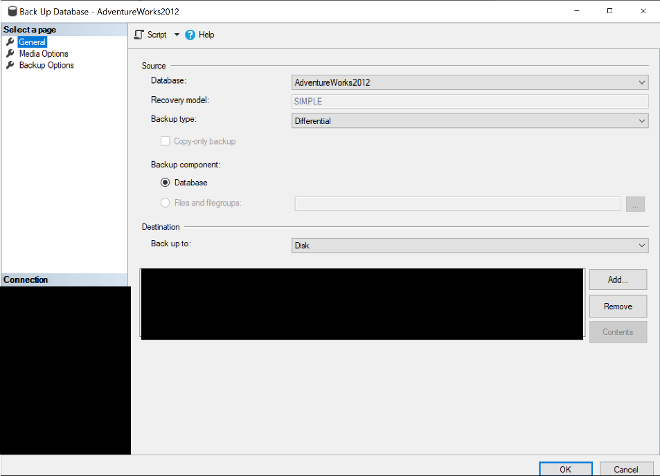
Using the GUI, right-click the database, go to Tasks, then choose Select Backup… For Backup Type, select Differential.

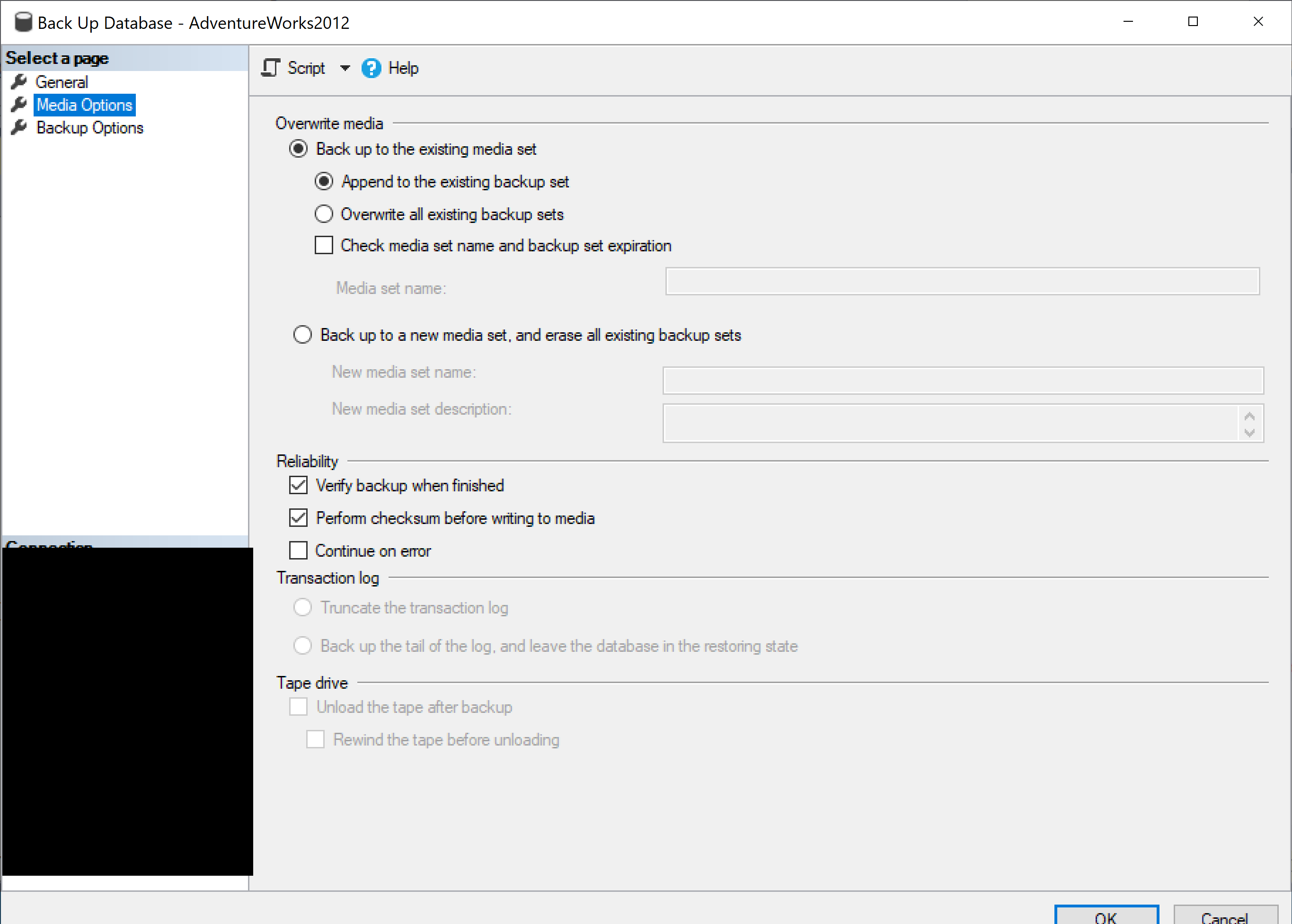
Fill out the Media Details as shown.

Change the expiration compression properties on the Backup options page.

TRANSACTION LOG backups

This is the magic behind the point-in-time restore option. This does just what you probably think it does – it backs up the transaction log (or “log”). It also clears the log (which prevents that log bloat that I spoke about before).

You may have thought that a FULL backup clears the transaction log and are wondering why it doesn’t. A FULL backup will take enough of the log to keep the database transactionally consistent, but SQL Server doesn’t know at that point if your database is in FULL recovery or SIMPLE. The recovery mode takes care of whether the transaction log undergoes CHECKPOINT, not the backups.

Using TSQL to do a log backup (Note: To do a log backup on AdventureWorks2012, which is in SIMPLE recovery, I had to put it into FULL recovery.).

BACKUP LOG [AdventureWorks2012]
TO  DISK = N'<filelocation, backup name>'
WITH NOFORMAT,
                        INIT,
                        NAME = N'AdventureWorks2012-Log Backup',
                        SKIP,
                        NOREWIND,
                        NOUNLOAD,
                        COMPRESSION,
                        STATS = 10;
GO
DECLARE @backupSetId AS INT;
SELECT @backupSetId = position
FROM msdb..backupset
WHERE database_name = N'AdventureWorks2012'
                        AND backup_set_id =
                (
                        SELECT MAX(backup_set_id)
                        FROM msdb..backupset
                        WHERE database_name = N'AdventureWorks2012'
                );
IF @backupSetId IS NULL
BEGIN
RAISERROR(N'Verify failed. Backup information for database ''AdventureWorks2012'' not found.', 16, 1);
END;
RESTORE VERIFYONLY
FROM DISK = N'<filelocation, backup name>'
WITH FILE = @backupSetId,
                NOUNLOAD,
                NOREWIND;
GO

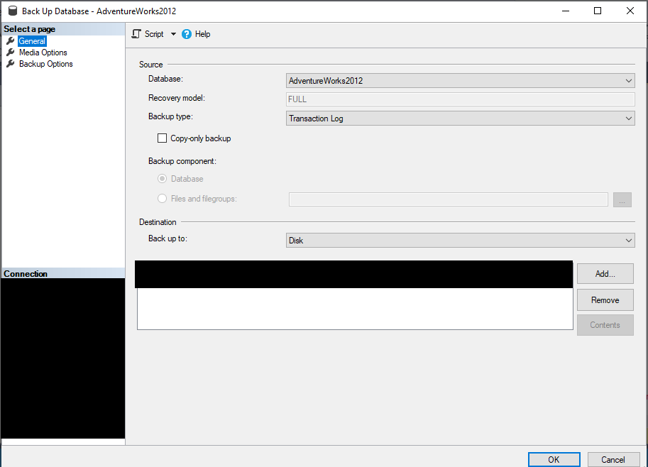
Using the GUI, launch the backup dialog as before, but this time, select Transaction Log as the backup type.

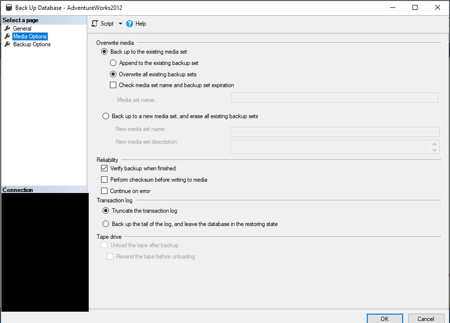
Change the Media Options as shown.

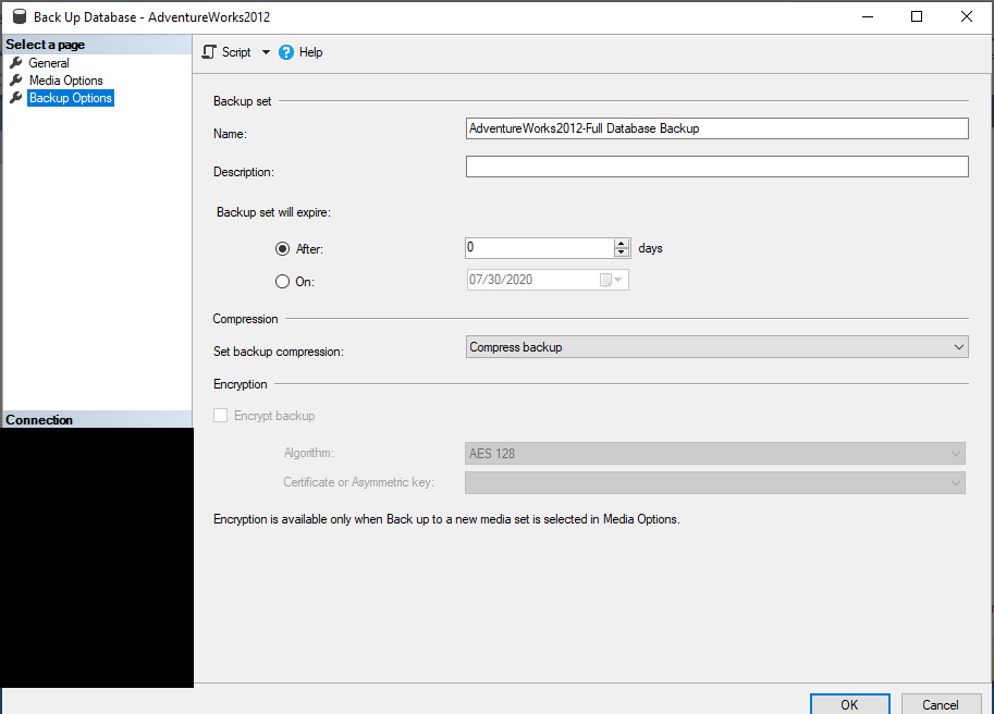
Change the backup options as necessary.

There are other backup/restore options, such as striped backups, filegroup backups, file backups, and partial backups (to name a few) which can help facilitate speedy restores in certain cases. I would recommend getting very comfortable with the basics first. Not sure where to look? Books Online has very good documentation, and there are other sites, such as Simple Talk and SQLSkills, that will help fill in the holes and answer questions as they occur.

Restore Strategies

You do backups in case you ever need to restore them. If you are a DBA for long enough, you’ll likely have to do this. I am only going to cover basic restores here; Books Online can walk you through more specialized restore options, such as filegroup, piecemeal and page restores.

FULL Restores

A full restore is the one that will take the longest, but it is the easiest to do. Just restore the closest FULL backup to your restore point. If you are only taking FULLs, you will only have one restore to do, so I will start with that.

Using TSQL, a basic FULL restore with no other backups involved would look like this:

USE [master];
RESTORE DATABASE [AdventureWorks2012]
FROM DISK = N'<location, name here>';
GO

Alternatively, you can use the GUI by right-clicking the database, then going to Tasks > Restore > Database, and clicking through the screens as you fill them in.

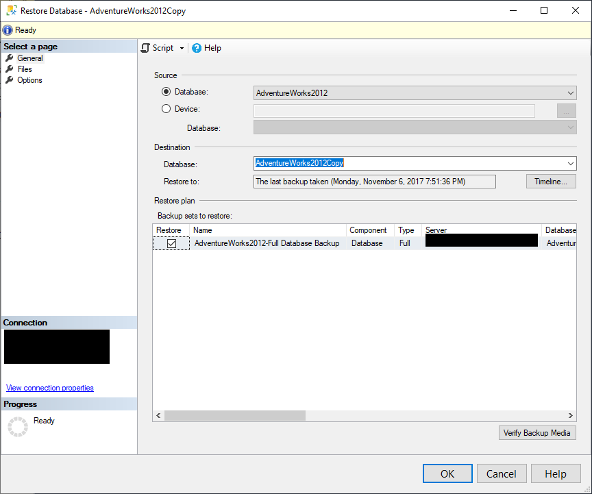
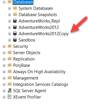
The GUI also makes it easy to make copies of the database. Returning to the Restore Database GUI, this time, I’ll make a copy of the AdventureWorks2012 database called AdventureWorks2012Copy by modifying the name in the Destination Database window:

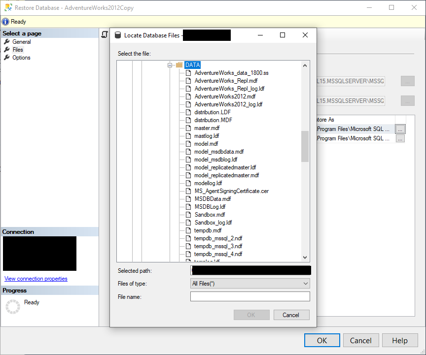
I could change the file locations if needed as well by going to the Files tab and clicking the ellipses next to the file names in the Restore As windows:

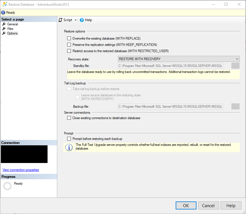
Finally, here is the Options tab:

Since this is a new database, I won’t be overwriting.

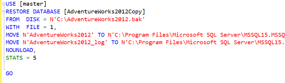
And, of course, by hitting the Script button at the top, SQL Server will make the script for me, which is convenient for documenting tickets, or better learning the syntax.

What does all of this code mean? It means that you are restoring a database called AdventureWorks2012Copy. FROM DISK shows the location. WITH FILE shows there is 1 file. MOVE shows where the files for the new database will wind up. NOUNLOAD is an old argument that just means that if the restore is happening from tape, the tape won’t be unloaded from the drive once you are done. The STATS argument is there to show your progress. In this case, it will update the messages tab for every five percent of the restore.

And here are the results.

I will edit some of the output for brevity, but it looks something like this:

5 percent processed.

10 percent processed.

15 percent processed.

20 percent processed.

…

95 percent processed.

100 percent processed.

Processed 24184 pages for database ‘AdventureWorks2012Copy’, file ‘AdventureWorks2012’ on file 1.

Processed 2 pages for database ‘AdventureWorks2012Copy’, file ‘AdventureWorks2012_log’ on file 1.

Converting database ‘AdventureWorks2012Copy’ from version 706 to the current version 904.

Database ‘AdventureWorks2012Copy’ running the upgrade step from version 706 to version 770.

RESTORE DATABASE successfully processed 24186 pages in 0.637 seconds (296.620 MB/sec).

Completion time: 2020-10-23T14:54:57.2214045-05:00

Notice the five percent stats and also the other messages. It shows the number of pages processed for the data and transaction log files, any upgrade conversions it does, and at what rate.

Restores with FULL and Differential Backups

Chances are you will need to have more than just a FULL backup restored. You are more likely to have backup chains involved, with a combination of FULL, differential, and log backups. These restores look a little different. To start as simply as possible, with a database that only uses a FULL and differential backup. One of the main things you want to keep in mind is that you have to tell SQL Server when it is done restoring. That is where the NORECOVERY/RECOVERY keywords come in. Using WITH NORECOVERY is like telling SQL Server, “Yes, restore that, but you are not done – there’s more!” The RECOVERY keyword tells SQL Server to finalize the restore. Here is an example of what that might look like:

USE [master];
RESTORE DATABASE [AdventureWorks2012]
FROM DISK = N'<location, name here>'
WITH NORECOVERY; --but wait, there is at least one more backup coming!
RESTORE DATABASE [AdventureWorks2012]
FROM DISK = N'<location, name here>'
WITH FILE = 2,
RECOVERY; -- Okay, you’re all done.

If you have a database in FULL recovery, using differential backups can dramatically cut down on the number of transaction log backups you need to restore. When practicing restores using diffs, you start with restoring the last FULL and then skip to the most recent diff to the restore point you have been given. For example, say you have a backup strategy of one FULL backup every day at 6 PM, differential backups every four hours round the clock, and transaction log backups every ten minutes. You are asked to restore a database to yesterday at 8 AM. You would go to the night before yesterday and find that 6 PM FULL backup. Then go to the 8 AM differential backup. That’s it. You don’t need any log backups; the diff will get you there all on its own. In this scenario, you’re done, saving you the pain of assembling a long chain of log backups!

To use another example, if you have a backup strategy of one daily FULL backup, diffs every six hours, and log backups every 15 minutes, then you could save up to 24 log backup restores by using a differential backup. The benefit of not having to restore the extra log backups is not primarily in time saved because log backups are generally pretty fast. Nor is the biggest benefit not having to assemble the log restore chain in the first place (although that is not to be underestimated). The big benefit is in reduced risk; if anything happened to go wrong with one of those extra log backups, you lose the data from that point on.

Restores with FULL, Differential, and Transaction Logs

When practicing your restores, a restore strategy for the log backups will look like this:

• Closest FULL backup before the restore time specified
• Closest DIFF backup to the restore time
• Every LOG backup between the DIFF and the end time. To get your point-in-time, simply use the WITH STOPAT command and specify a time.

This code uses TSQL to restore a FULL, a diff, and two log backups:

USE [master];
RESTORE DATABASE [AdventureWorks2012]
FROM DISK = N'<location, name here>'
WITH NORECOVERY;
GO
RESTORE DATABASE [AdventureWorks2012]
FROM DISK = N'<location, name here>'
WITH FILE = 2,
NORECOVERY;
GO
RESTORE LOG [AdventureWorks2012]
FROM DISK = N'<location, name here>'
WITH NORECOVERY;
GO
RESTORE LOG [AdventureWorks2012]
FROM DISK = N'<location, name here>'
WITH RECOVERY; 
GO

Or, for a point-in-time restore:

USE [master];
RESTORE DATABASE [AdventureWorks2012]
FROM DISK = N'<location, name here>'
WITH NORECOVERY;
GO
RESTORE DATABASE [AdventureWorks2012]
FROM DISK = N'<location, name here>'
WITH FILE = 2,
NORECOVERY;
GO
RESTORE LOG [AdventureWorks2012]
FROM DISK = N'<location, name here>'
WITH NORECOVERY;
GO
RESTORE LOG [AdventureWorks2012]
FROM DISK = N'<location, name here>'
WITH NORECOVERY, STOPAT = ‘January 1, 2020 8:03 AM’;
RESTORE DATABASE AdventureWorks2012 WITH RECOVERY; 
GO

There is an extra special bit of magic called a tail-of-the-log backup, which is one last log backup, allowing you to get as close to the present moment as it possibly can, should you need it. You’ll find it in the GUI for the restores.

Restore Practice

You can have the best set of backups around, but if you haven’t practiced doing restores (and especially if you don’t have an idea of how long they take), it can mean unexpected downtime and money for the business, and a bad day at the office for you.

I’ve shown you how to use TSQL or the GUI to do restores, but if you want to meet the numbers on your SLA, you will want to automate your backup and restore processes. This means either using backup software such as Redgate’s SQL Backup or using a free solution such as Ola Hallengren’s Backup Solution and writing your automated restore process. Whatever direction you choose, it should be well tested and vetted before you adopt it.

So, how to test your backups and restores? This is, after all, the whole reason for having backups in the first place – to have them in case you need to do a restore. Having a staging environment is a perfect chance to do this. Write a process to blow away the databases from the previous evening and restore your previous night’s backups. Then run a DBCC CHECKDB on them. This process will show that as of the time of your test, the backup is good. Lather, rinse, repeat.

Layering Your Backup Strategy

You have tested your backups by restoring them. You have confirmed that you can restore in the time allotted by your SLA. You have congratulated yourself and breathed a sigh of relief. You’re all good now, right?

No, not necessarily.

Why would that not be enough? Well, can something happen on the file share to corrupt that backup later on? Possibly. This is why you want a layered backup strategy.

As a DBA, you always want to be thinking, What if it breaks? This is one job where you are paid to scare yourself a little. This is never more true than with your backups. Having a layered backup strategy allows you to have a Plan B, a Plan C – as many plans as you think are necessary. For instance, supplementing your backups with server-level snapshots provides a little more security. You may not have the same restore-point flexibility with server-level snapshots, but with this combination, you can significantly reduce your chances of being caught tongue-tied when the alarm bells start going off. You can also copy off your backups to another file share or location. The point is not to put all of your eggs in one basket.

Conclusion

Understanding how recovery models work, what backup options are available to you, and how to use that knowledge to ensure that you can deliver the right data as quickly as possible is one of the most fundamental tools you will have in your tool belt as a DBA. Understanding the concepts laid out here is the beginning of that knowledge for you. As time goes on, you will learn more advanced concepts as the needs of your business dictate, or as your curiosity leads you to greater professional growth. This is only the beginning but learning these things and being able to do them well will be of great benefit as you strive to get the job, or grow in the profession.

 

The post DBA in training: Backups, SLAs, and restore strategies appeared first on Simple Talk.

from Simple Talk https://ift.tt/38wvtVD
via

Git in action

The series so far:

1. How we ended up with git
2. Git anatomy
3. Git in action

Git is a shell of code hosted in an operating system and capable of processing commands to track and version the content of a tree of directories. Git can work on a single machine under the control of a single user, but it is designed to connect multiple instances running on physically distant machines. More, any repository being tracked locally can be connected to a remote repository. Data can be transferred between local and remote repositories using the set of commands made aptly available.

Git was born to track and version source code files, but by no means it is limited to text files written in some programming language. Although managing the codebase of one software project is the most common use case, nothing stops you from using Git to manage the various stages of a book project or a graphic work. As long as your work creates and updates digital files, Git is here to help.

In this article, you’ll play with the basic Git commands and see how to use them to track and version the constituent files of a sample project. The article focuses on the command-line interface because it’s the quickest way to get a firm grasp of the Git workflow.

Initializing a Repository

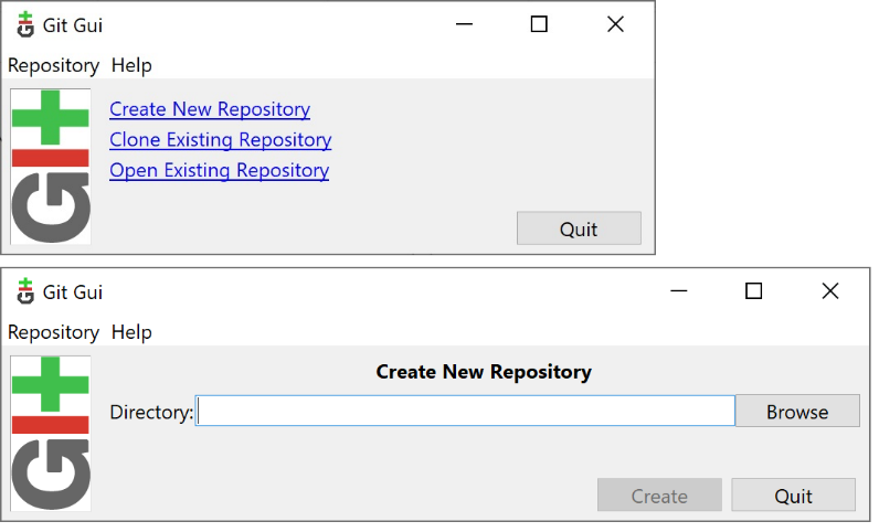
Once installed on a computer, Git can be used interchangeably through a number of programming interfaces, including Git Bash and Git GUI. On the Windows platform, you can also have two more options to choose: Git CMD and PowerShell. Git Bash is the native command-line interface of Git whereas Git GUI is a visual shell capable of the same basic operations. To launch it, just type git gui in a command window.

When you run Git GUI on a non-monitored directory, it shows the main menu: creating a new repository, cloning, or just opening an existing repository.

To create a new repository, you need to enter the path to the directory. If you want to do it from the command line, then the command to type in is the following:

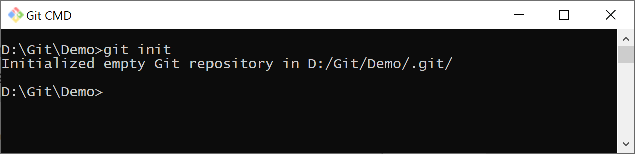
git init

Here’s how the system would handle it in Git CMD—the dedicated Windows console shell for Git.

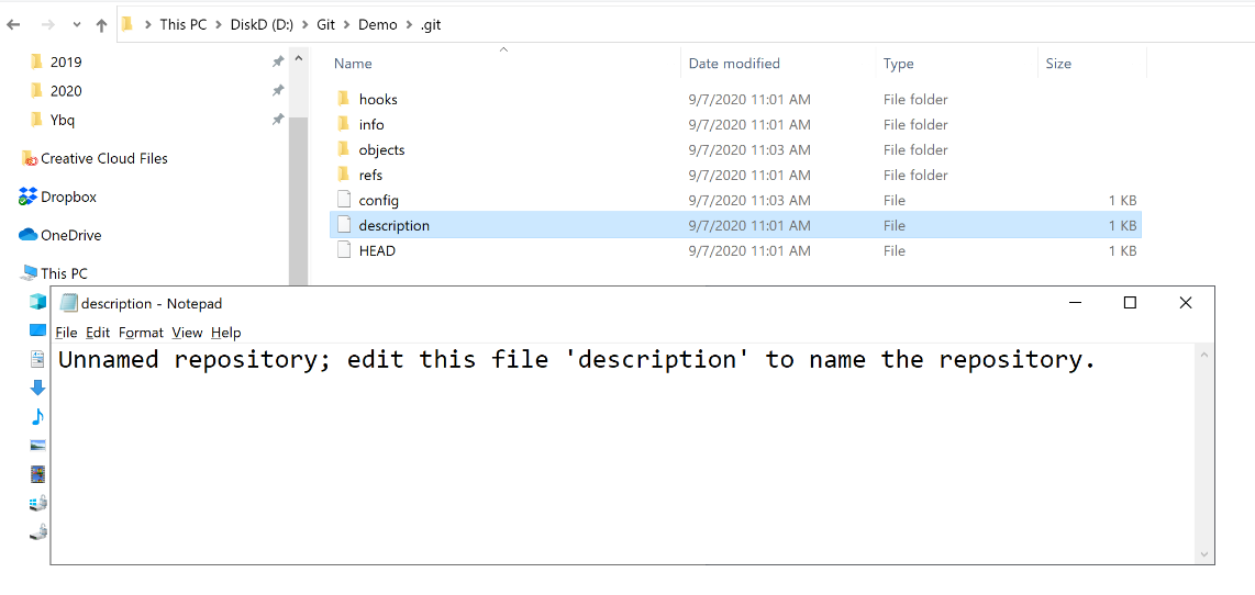
The net effect of creating a new Git repository on a file system directory is the creation of a hidden .git subfolder where several configuration files are stored telling the runtime how to deal with what happens within the boundaries of the subtree. In Windows, to snoop into the hidden .git folder, you turn on the Hidden Files view in Windows Explorer and head to the folder. Here’s what you see.

A number of files and subfolders contain all that’s needed to run the Git monitor on the content. In particular, the file named description contains the public name of the repository. You can edit its content through a text editor to give it a meaningful description. The HEAD file you can see in the figure is also worth some remarks. The contents of the HEAD file refer to the current state of the files that you have in the local repository. It’s a pointer to the copy of the files you’re currently working with and the next you’ll save back to the repository.

There are a couple of terms frequently used when explaining the purpose of the HEAD file: one is commit, and the other is checkout. With the term commit, one refers to the state of the stored files at a given time, when the git commit command (namely, a save-changes command) was issued. HEAD is, therefore, a pointer to the latest version of the files. With the term checkout, instead, one refers to the action of switching between different versions of a Git entity such as individual files, entire commits, or branches. When created, a branch is a fork of the current committed state.

In a freshly created and empty repository, the HEAD file contains the following:

ref: refs/heads/master

It reads like the HEAD references the file refs/heads/master, which is expected to contain the unique identifier (hash) of the most recent commit on the primary (master) branch. In an empty repository, the master file in the refs/heads directory doesn’t just exist.

Now learn how it changes when adding some content to the repository.

Populating a Repository

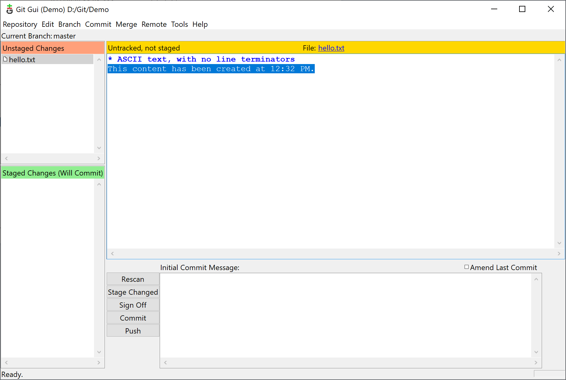
Create a text file in the monitored folder, say hello.txt, and give it some default content such as the timestamp to easily track it back. If you open Git GUI on the sample folder, you should see what’s in the figure.

On the left side of the window, you see two docked lists showing unstaged and staged changes. Unstaged changes refer to files in the folder that are detected as new or modified but have not yet been added to the list of changes you intend to commit at some point in time. The content you commit is any content you may possibly switch back in the future or may use as the starting point for new and independent lines of development (branches). As an author, if you know that the current stage of the hello.txt file is destined to change because, in some way transitory or incomplete, you keep it in the unstaged list. On the other hand, if you believe that the file will need to make it to the next commit, then you add it to the stage list. You can keep editing it, but next time you commit the state of the file will be permanently saved and identified with a unique hash.

To move the file to the list of staged changes from the command line, you use the command:

git add hello.txt

You can also click Stage changed in the git GUI app.

To remove a file from the list of pending changes to be committed later, you use the command:

git reset hello.txt

When issuing the git reset command if you don’t specify the name of the file then all pending changes are removed from the list of staged changes. Once you commit pending changes that have been stage, use the git commit command to perform the commit. You’ll also have to supply a commit message for each commit

git commit hello.txt -m"Initial commit"

The git log command will let you inspect the history of the repository.

Each commit is given a unique identifier that unambiguously references the chunk of changes being made. The log command has many flavors, the most relevant of which as summarized below.

git log	Displays the entire history of the repository
git log -n N	Displays last N commits
git log –oneline	Displays the entire history of the repository in a compact way, only one line per commit
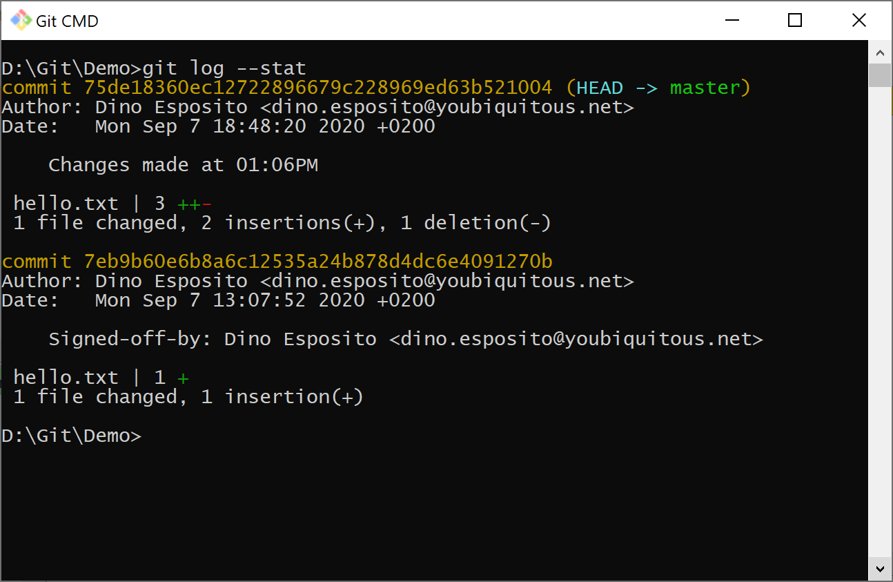
git log –stat	Displays also which files were altered and the relative number of lines that were added or deleted
git log –author=pattern	Displays the commits by a given author

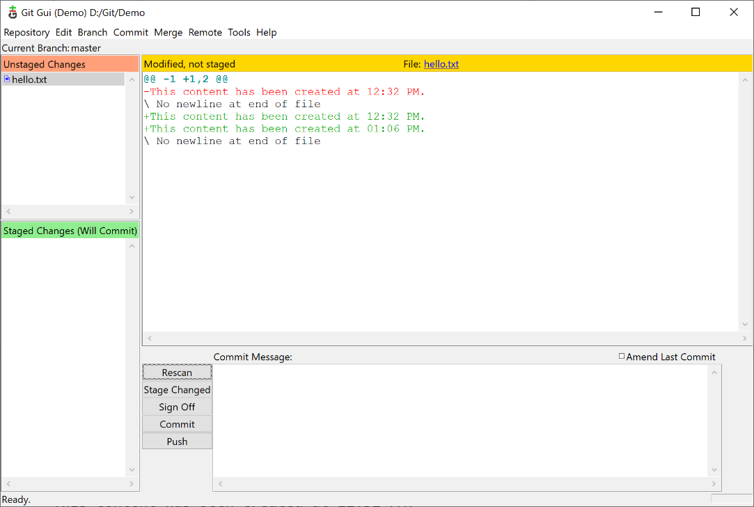
Now see what happens when another change is made to the same hello.txt file. The Git GUI application now displays the following. Note that you may have to click Rescan to see the changes.

The unstaged change is described as the removal of the line below.

And the addition of the following lines:

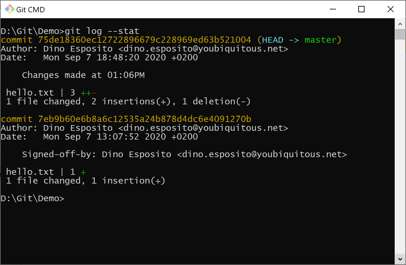
After moving changes to the staging area and placing a commit command you get the following log.

The log shows the two commits that have occurred, each identified by its unique GUID. The head of the repository points to the master (primary) branch. The last commit is labeled as “Changed made at 01:06PM” which was the text of the commit message. The notes of the latest commit also indicate that one file was changed because some content was inserted.

When it comes to inspecting the content of a repository, you might also want to look into the git status command. The command represents the state of the directory and the staging area with pending changes. The output shows which changes have been slated for commit and which have not. It also shows which files in the working folder are not currently tracked by Git. Note that the output of the status command does not include any information about the historical sequence of commits.

Selecting Files to Track

By default, all files created in a Git-tracked subtree are subject to the action of the tool. It doesn’t mean, however, that you can’t cherry-pick some files and tell Git to ignore them when performing a commit. A text file named .gitignore, placed in the root directory of the repository, instructs the Git engine about files and folders to ignore during a commit. Note that the .gitignore file does not affect files already in the repository. Each line of the .gitignore file defines a pattern for files to ignore. Usually, the file affects a single repository. However, you can also define global ignore rules, for all repositories on a machine, as below:

git config --global core.excludesfile ~/.gitignore_global

The ignore file itself is treated as a file in the repository, and you might want to commit it if you intend to share the ignore rules with anybody who may happen to clone your repository later.

The content of a .gitignore file is critical. Here’s a very basic example of what you can put it in it. In brief, it contains a list of wildcard paths and patterns for locating the files in the subtree to ignore.

# Ignore all files whose name matches "unused"
unused.*

Any line that begins with # is treated as a comment and ignored. You can find several predefined and validated examples of ignore files at https://github.com/github/gitignore and can create a starter ignore file for a given operating system, IDE or programming language visiting the https://gitignore.io web site.

As mentioned, all files already checked in at the time the ignore rules are defined are unaffected. In this case, you must untrack them from Git. Here’s the command you need:

git rm --cached filename

Ignore rules are not the only way to select which files will be considered for the commit and which not. Another substantially equivalent mechanism passes through the use of the exclude file. When a Git repository is created, a text file named exclude is automatically created in the .git/info folder. Its content is equivalent to .gitignore and follows the same syntax rules. The difference between ignore and exclude rules is that ignore rules are devised to be shared among project members having access to the repository, whether remote or cloned. Exclude rules remain local to the repository and are meant to be mostly personal rules.

Going to a Specific Revision

The crucial benefit of Git is that it keeps track for you of multiple revisions of the same files. From the command line, the git log command lets you see the list of revisions, each identified by a hash code. How would you access a specific revision of the project that was created a while back? You use the checkout command with the hash code of the commit.

git checkout hashcode

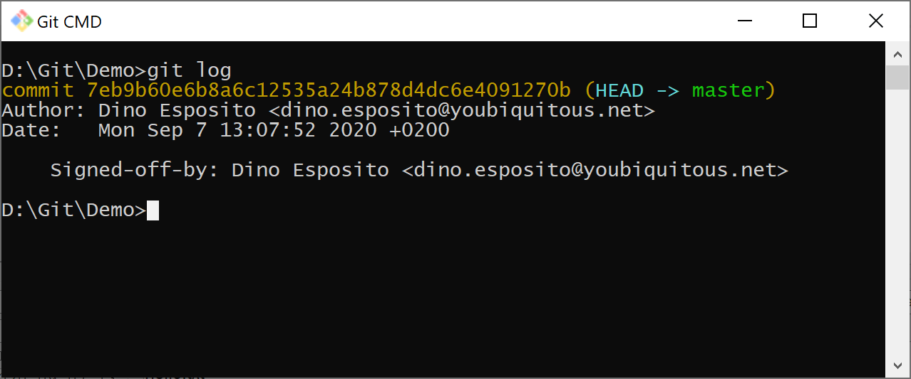
When running the git log command, you see the hash code 7eb9b60… referencing the first sample commit where the hello.txt file contained only one line of text.

Here’s the command to switch the repository back to on older state and gain access to the files in the repository at the time of the given commit.

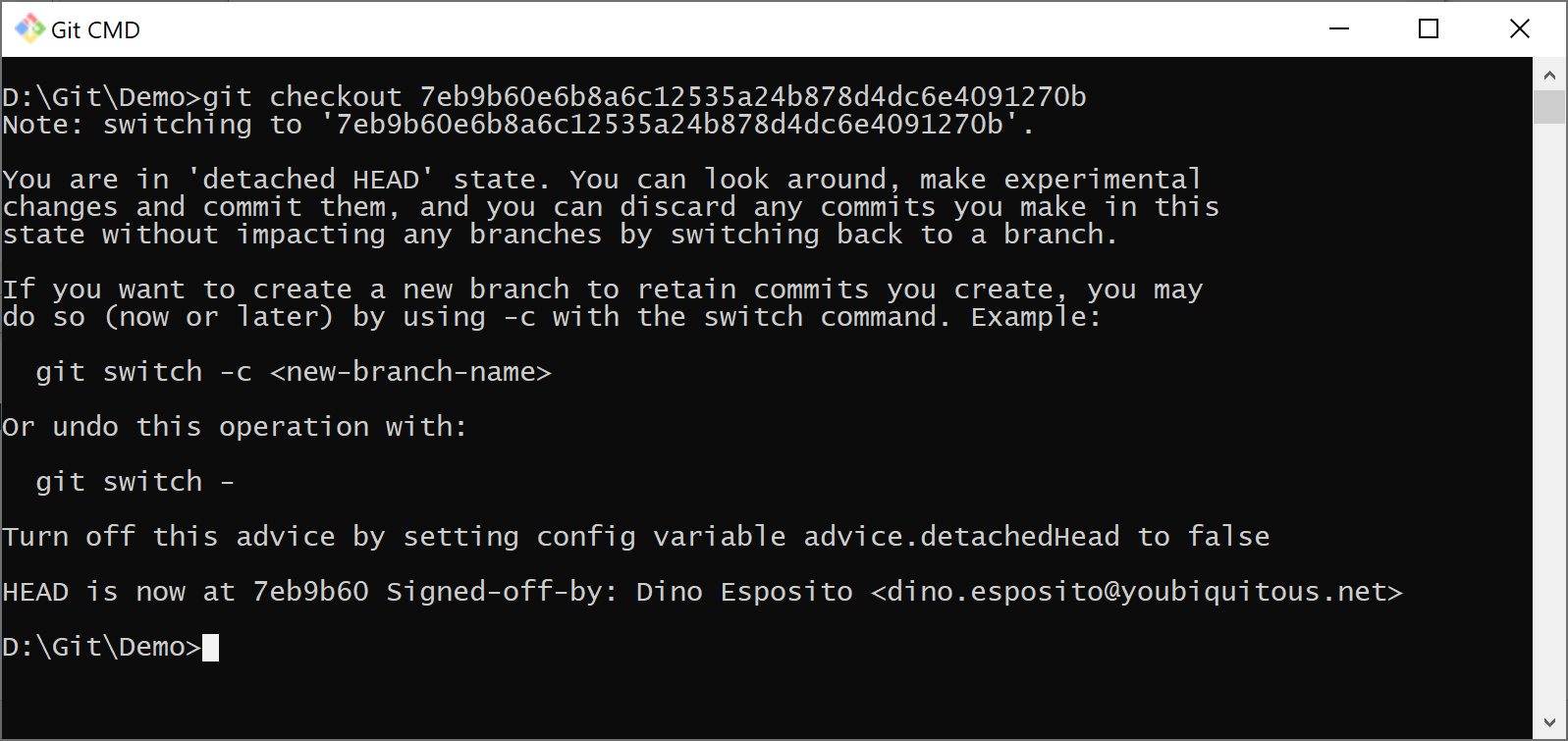
git checkout 7eb9b60e6b8a6c12535a24b878d4dc6e4091270b

Here’s the output.

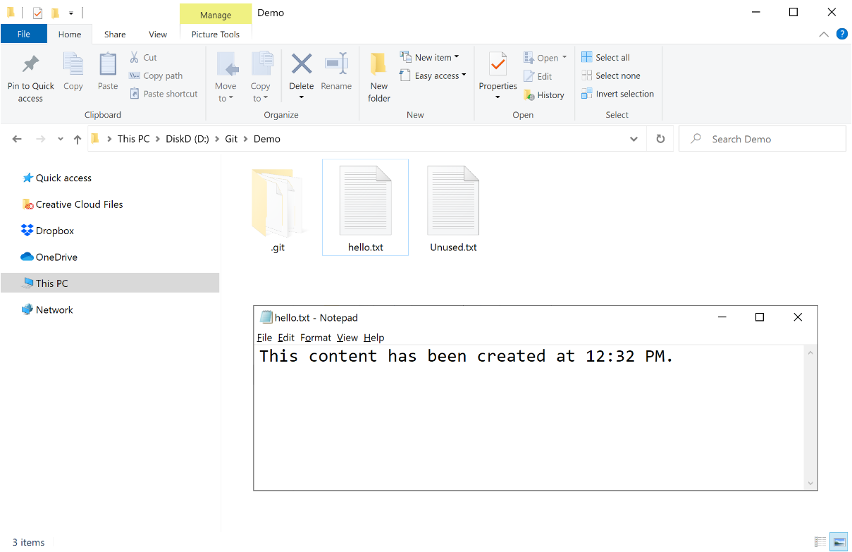
The Windows folder now shows a hello.txt file and no other tracked file like .gitignore. In the figure below, you see the unused.txt file because it’s marked to be ignored by Git. The content of the hello.txt is the expected old one.

When Git receives the checkout command, it then places all files in the specified revision in the working folder. In this case, it just replaced the latest hello.txt with an older version of it. What you do next depends on the reason that led you to check out an older version of the project. If you want to save a copy of the files, all you do is copy the file to a different folder and go. The new folder is disconnected from Git (or it could even be a new distinct Git repository) and can be managed as appropriate.

However, when you checkout an older commit the state of repository changes, as the output of the command shows.

git checkout 9605a5c08

After the checkout of a commit, the repository is in a detached HEAD state. The detached HEAD state is legitimate but potentially dangerous. The reason is that when you checkout a specific commit from a repository, the HEAD pointer—namely, the reference to the current working revision in the repository, is not updated. This means that the files in the working area of the repository and the pointer are no longer in sync. Is this a problem? Well, the moment you edit any of the checked-out files and force to commit changes back, these changes won’t belong to any revision and will likely be lost if you later check out another revision. In other words, commits out of a detached HEAD state are not tracked and can hardly be retrieved later. The only way to check them outat a later time is by remembering the exact hash code—a GUID—of the latest commit. Here’s an example:

git checkout 4505ddc08

To revert to the master repository that you left when checked out an earlier commit, use the command below. Note though that the command switches back the HEAD pointer to master and loses all of the intermediate changes on the older commit.

git checkout master

To avoid the detached HEAD issue entirely, you should use another key concept of Git—the branch. The branch is an independent and fully supported line of development of the project. It has a name and can be created upon checkout. Branching is a crucial topic, though, and deserves its own space to be appropriately described. I’ll get into that in the next article.

Summary

In the end, the Git workflow is straightforward. You initialize a repository on an existing folder, you work on it creating and editing files, track files you’re interested, and commit changes. Any committed change represents the snapshot of the project you want to preserve, or return to, later. To switch back to a previous version and to inspect the status of the repository, you have other dedicated commands. This is the essence of Git and to perform all these actions, you can count on a number of visual and command-line tools. In the next article of this series, I’ll focus on a few more specific and advanced Git commands such as branch, stash and merge.

 

The post Git in action appeared first on Simple Talk.

from Simple Talk https://ift.tt/3ke3CLY
via

Unwrapping JSON to SQL Server Tables

If you know the structure and contents of a JSON document, then it is possible to turn this into one or more relational tables, but even then I dare to you claim that it is easy to tap in a good OpenJSON SELECT statement to do it. If you don’t know what’s in that JSON file, then you’re faced with sweating over a text editor trying to work it all out. You long to just get the contents into a relational table and take it on from there. Even then, You’ve got several struggles before that table appears in the result pane. You must get the path to the tabular data correct, you have to work out the SQL Datatypes, and you need to list the full panoply of keys. Let’s face it: it is a chore. Hopefully, all that is in the past with these helper functions.

What about being able to do this, for example …

EXECUTE TablesFromJSON @TheJSON= N'[
    {"name":"Phil", "email":"PhilipFactor@geeMail.com"},
    {"name":"Geoff", "email":"Geoff2435@geeMail.com"},
    {"name":"Mo", "email":"MoHussain34@geeMail.com"},
    {"name":"Karen", "email":"KarenAlott34@geeMail.com"},
    {"name":"Bob", "email":"bob32@geeMail.com"}
]'

 

…and getting this?

Or if there is more than one table somewhere there…

DECLARE @json NVARCHAR(MAX) =
  N'{
        "id": "0001",
        "type": "donut",
        "name": "Cake",
        "ppu": 0.55,
        "batters":
                {
                        "batter":
                                [
                                        { "id": "1001", "type": "Regular" },
                                        { "id": "1002", "type": "Chocolate" },
                                        { "id": "1003", "type": "Blueberry" },
                                        { "id": "1004", "type": "Devil''s Food" }
                                ]
                },
        "topping":
                [
                        { "id": "5001", "type": "None" },
                        { "id": "5002", "type": "Glazed" },
                        { "id": "5005", "type": "Sugar" },
                        { "id": "5007", "type": "Powdered Sugar" },
                        { "id": "5006", "type": "Chocolate with Sprinkles" },
                        { "id": "5003", "type": "Chocolate" },
                        { "id": "5004", "type": "Maple" }
                ]
}';
EXECUTE TablesFromJson @JSON

 

You may not want table results straight out of your JSON: I’m really just showing off, but I’m going to describe some routines that are useful to me for dealing with JSON import. Your requirements may be more subtle.

The first stage is to get a good representation of a json document so you can work on it in SQL. I do this with a multi-statement table-valued function, but you’ll see that it is a mostly pretty simple unwrapping of the json document. Built into it is a way of gauging the most appropriate SQL Datatype for each value. Unless you adopt JSON Schema, there is no onus on being consistent in assigning values to keys, so you have to test every simple value (i.e. everything other than arrays or objects)

CREATE OR alter FUNCTION [dbo].[UnwrapJson]
/**
summary:   >
  This multi-statement table-valued function talkes a JSON string and
  unwraps it into a relational hierarchy table that also retains
  the path to each element in the JSON document, and calculates the
  best-fit sql datatype fpr every simple value
Author: Phil Factor
Revision: 1.0
date: 1 Nov 2020
example:
  - SELECT * FROM UnwrapJson (N'[  
    {"name":"Phil", "email":"PhilipFactor@gmail.com"},  
    {"name":"Bob", "email":"bob32@gmail.com"}  
    ]')
returns:   >
  id, level, [key], Value, type, SQLDatatype, parent, path
 
**/    
(
    @JSON NVARCHAR(MAX)
)
RETURNS @Unwrapped TABLE 
  (
  [id] INT IDENTITY, --just used to get a unique reference to each json item
  [level] INT, --the hierarchy level
  [key] NVARCHAR(100), --the key or name of the item
  [Value] NVARCHAR(MAX),--the value, if it is a null, int,binary,numeric or string
  type INT, --0 TO 5, the JSON type, null, numeric, string, binary, array or object
  SQLDatatype sysname, --whatever the datatype can be parsed to
  parent INT, --the ID of the parent
  [path] NVARCHAR(4000) --the path as used by OpenJSON
  )
AS begin
INSERT INTO @Unwrapped ([level], [key], Value, type, SQLDatatype, parent,
[path])
VALUES
  (0, --the level
   NULL, --the key,
   @json, --the value,
   CASE WHEN Left(ltrim(@json),1)='[' THEN 4 ELSE 5 END, --the type
   'json', --SQLDataType,
   0 , --no parent
   '$' --base path
  );
DECLARE @ii INT = 0,--the level
@Rowcount INT = -1; --the number of rows from the previous iteration
WHILE @Rowcount <> 0 --while we are still finding levels
  BEGIN
    INSERT INTO @Unwrapped ([level], [key], Value, type, SQLDatatype, parent,
    [path])
      SELECT [level] + 1 AS [level], new.[Key] AS [key],
        new.[Value] AS [value], new.[Type] AS [type],
-- SQL Prompt formatting off
/* in order to determine the datatype of a json value, the best approach is to a determine
the datatype that can be parsed. It JSON, an array of objects can contain attributes that arent
consistent either in their name or value. */
       CASE 
        WHEN new.Type = 0 THEN 'bit null'
                WHEN new.[type] IN (1,2)  then COALESCE(
                  CASE WHEN TRY_CONVERT(INT,new.[value]) IS NOT NULL THEN 'int' END, 
                  CASE WHEN TRY_CONVERT(NUMERIC(14,4),new.[value]) IS NOT NULL THEN 'numeric' END,
                  CASE WHEN TRY_CONVERT(FLOAT,new.[value]) IS NOT NULL THEN 'float' END,
                  CASE WHEN TRY_CONVERT(MONEY,new.[value]) IS NOT NULL THEN 'money' END,
                  CASE WHEN TRY_CONVERT(DateTime,new.[value],126) IS NOT NULL THEN 'Datetime2' END,
                  CASE WHEN TRY_CONVERT(Datetime,new.[value],127) IS NOT NULL THEN 'Datetime2' END,
                  'nvarchar')
           WHEN new.Type = 3 THEN 'bit'
           WHEN new.Type = 5 THEN 'object' ELSE 'array' END AS SQLDatatype,
        old.[id],
        old.[path] + CASE WHEN old.type = 5 THEN '.' + new.[Key] 
                                           ELSE '[' + new.[Key] COLLATE DATABASE_DEFAULT + ']' END AS path
-- SQL Prompt formatting on
      FROM @Unwrapped old
        CROSS APPLY OpenJson(old.[Value]) new
          WHERE old.[level] = @ii AND old.type IN (4, 5);
    SELECT @Rowcount = @@RowCount;
    SELECT @ii = @ii + 1;
  END;
  return
END
go

 

Now, you have the document as a table. You can now unpick this in several ways, but we want to get all the tables that are embedded in the json. These are generally represented as arrays of objects, each of these objects representing a ‘document’ or ‘row’. In JSON, you can, of course, have an object or array as a value for one of the keys within the object; equivalent to storing xml or json in a relational column- but we’re after the simple columns.

Because we are looking for the tables, we can get a quick listing of them. (in reality, you’d probably only want a sample of each if you’re just browsing)

First we place the output of dbo.unwrapJSON into a temporary table. I’ve chosen #jsonObject. Now we can see the rows, if there are any table structures within the JSON.

SELECT parent.path AS [TheTable] ,grandchild.*
      FROM
        (SELECT path, id FROM #jsonObject WHERE type = 4) Parent --start with an array
        INNER JOIN #jsonObject Child
          ON Child.parent = Parent.id AND child.type IN (4, 5) --either array or object
        INNER JOIN #jsonObject GrandChild
          ON GrandChild.parent = Child.id AND GrandChild.type NOT IN (4, 5)

 

Well, that’s fine as far as it goes, but it doesn’t go far enough. What I want is the OpenJSON query that I can execute to get the actual result.

Here is an inline table function that does just that, using the expression I’ve just shown you.

CREATE OR alter FUNCTION [dbo].[OpenJSONExpressions]
/**
summary:   >
  This inline table-valued function talkes a JSON string and
  locates every table structure. Then it creates an OpenJSON
  Statement that can then be executed to create that table
  from the original JSON.
Author: Phil Factor
Revision: 1.0
date: 1 Nov 2020
example:
  - SELECT * FROM OpenJSONExpressions (N'[  
    {"name":"Phil", "email":"PhilipFactor@gmail.com"},  
    {"name":"Bob", "email":"bob32@gmail.com"}  
    ]')
returns:   >
  expression
 
**/    
(
   @JSON NVARCHAR(MAX)
    
)
RETURNS TABLE AS RETURN
(
WITH UnwrappedJSON (id, [level], [key], [Value], [type], SQLDatatype, parent,
                   [path]
                   )
AS (SELECT id, [level], [key], [Value], [type], SQLDatatype, parent, [path]
      FROM dbo.UnwrapJson(@json) )
  SELECT 'Select * from openjson(@json,''' + path + ''')
WITH ('  + String_Agg(
                       [name] + ' ' + datatype + ' ' --the WITH statement
-- SQL Prompt formatting off
   + case when datatype='nvarchar' then '('+length+')' 
     WHEN datatype='numeric' then  '(14,4)' ELSE '' end,', ')
   WITHIN GROUP ( ORDER BY  TheOrder  ASC  )    +')' as expression
-- SQL Prompt formatting on
    FROM
      (
      SELECT Parent.path, GrandChild.[key] AS [name], Min(GrandChild.id) AS TheOrder,
            Max(GrandChild.SQLDatatype) AS datatype,
        Convert(NVARCHAR(100), Max(Len(GrandChild.Value))) AS length
        FROM
          (SELECT path, id FROM UnwrappedJSON WHERE type = 4) Parent
          INNER JOIN UnwrappedJSON Child
            ON Child.parent = Parent.id AND child.type IN (4, 5)
          INNER JOIN UnwrappedJSON GrandChild
            ON GrandChild.parent = Child.id AND GrandChild.type NOT IN (4, 5)
        GROUP BY Parent.path, GrandChild.[key]
      ) TheFields
    GROUP BY path
        )
GO

So we try it out with some JSON that has two table in it.

SELECT * FROM OpenJSONExpressions (
  N'{"employees":[  
    {"name":"Mo", "email":"mojaiswal@gmail.com", "StartDate":"2012-11-07T18:26:20"},  
    {"name":"Bob", "email":"bob456@gmail.com", "StartDate":"2015-06-20"},  
        {"name":"Phil", "email":"PhilipFactor@gmail.com", "StartDate":"2015-08-01T08:05:20"},
    {"name":"Susan", "email":"Su87@me.com", "StartDate":"2012-13-07"}  
],"Customers":[  
    {"name":"The Kamakaze Laxative Company", "contact":"Karen", "email":"Enquiries@KLCEnterprises.co.uk", "CustomerSince":"2012-11-07"},  
    {"name":"GreenFence Softwear limited", "contact":"Dick", "email":"Bob@GreenFenceSoftwear.com", "CustomerSince":"2015-06-20"},  
        {"name":"Grimm and Grivas, Solicitors",  "contact":"Jaz", "email":"GrimmGrivas@gmail.com", "CustomerSince":"2015-08-01T08:05:20"}
]
}  ')

 

From this we get the result …

Which are the following queries…

Select * from openjson(@json,'$.Customers')
WITH (name nvarchar (29), contact nvarchar (5), email nvarchar (30), CustomerSince Datetime2 )

Select * from openjson(@json,'$.employees')
WITH (name nvarchar (5), email nvarchar (22), StartDate nvarchar (19))

Well, those look suspiciously-executable; so we’ll do just that, in the following procedure

go
CREATE PROCEDURE TablesFromJSON @TheJSON NVARCHAR(MAX)
/**
summary:   >
  This procedure returns a table for every one found  in a JSON 
  string 
Author: Phil Factor
Revision: 1.0
date: 1 Nov 2020
example:
  - EXECUTE TablesFromJSON @TheJSON= N'[  
    {"name":"Phil", "email":"PhilipFactor@geeMail.com"},  
    {"name":"Geoff", "email":"Geoff2435@geeMail.com"},
    {"name":"Mo", "email":"MoHussain34@geeMail.com"},
    {"name":"Karen", "email":"KarenAlott34@geeMail.com"},
        {"name":"Bob", "email":"bob32@geeMail.com"}   
    ]'
returns:   >
  expression
 
**/    
AS
DECLARE @expressions TABLE (id INT IDENTITY, TheExpression NVARCHAR(MAX));
INSERT INTO @expressions (TheExpression)
  SELECT expression FROM OpenJSONExpressions(@TheJSON);
DECLARE @RowCount INT = -1, @ii INT = 1, @expressionToExcecute NVARCHAR(MAX);
WHILE @RowCount <> 0
  BEGIN
    SELECT @expressionToExcecute = TheExpression FROM @expressions WHERE id = @ii;
    SELECT @RowCount = @@RowCount;
    SELECT @ii = @ii + 1;
    IF @RowCount > 0
      EXECUTE sp_executesql @expressionToExcecute, N'@JSON NVARCHAR(MAX)',
        @JSON = @TheJSON;
  END;
GO 
So we try it out…
EXECUTE TablesFromJSON  
  N'{"employees":[  
    {"name":"Mo", "email":"mojaiswal@gmail.com", "StartDate":"2012-11-07T18:26:20"},  
    {"name":"Bob", "email":"bob456@gmail.com", "StartDate":"2015-06-20"},  
        {"name":"Phil", "email":"PhilipFactor@gmail.com", "StartDate":"2015-08-01T08:05:20"},
    {"name":"Susan", "email":"Su87@me.com", "StartDate":"2012-13-07"}  
],"Customers":[  
    {"name":"The Kamakaze Laxative Company", "contact":"Karen", "email":"Enquiries@KLCEnterprises.co.uk", "CustomerSince":"2012-11-07"},  
    {"name":"GreenFence Softwear limited", "contact":"Dick", "email":"Bob@GreenFenceSoftwear.com", "CustomerSince":"2015-06-20"},  
        {"name":"Grimm and Grivas, Solicitors",  "contact":"Jaz", "email":"GrimmGrivas@gmail.com", "CustomerSince":"2015-08-01T08:05:20"}
]
}  '

 

And voila! Two results.

So there we have it. I have to admit that the TablesFromJSON procedure isn’t quite so practical as I’d like because it is impossible to get more than one result from a stored procedure within SQL (no problem from an application, of course). It turned out to be very useful in testing all the code out, though.

I use all three routines. I hope that they’re useful to you. If you spot a bug, then let me know in the comments.

These are stored with my JSON/SQL Server routines here Phil-Factor/JSONSQLServerRoutines

• UnwrapJSON.sql
• TablesFromJSON.sql
• OpenJSONExpressions.sql

 

The post Unwrapping JSON to SQL Server Tables appeared first on Simple Talk.

from Simple Talk https://ift.tt/38iKHx0
via

Saving money with Log Analytics

Azure Monitor and Log Analytics are a very important part of Azure infrastructure. In my opinion, the adoption of these tools should start before a company starts its migration to azure. Using these tools over on premises servers can generate a performance baseline to be used when migrating the servers, ensuring the environment will be improving.

However, it needs to be a careful implementation, if you choose to take the easier way, you may cost some buckets to your company pocket.

The biggest example I noticed was the alert system. This system is an essential part not only of these tools but of the azure infrastructure as a hole, but you need to take care with the expenses. When you use the alert system you have some options to choose and, among them, Log or Metrics.

The log option means you need to build a Kusto query to retrieve an information from the Log Analytics storage, while the Metrics means you will define one metric you are interested on and Log Analytics will do the rest.

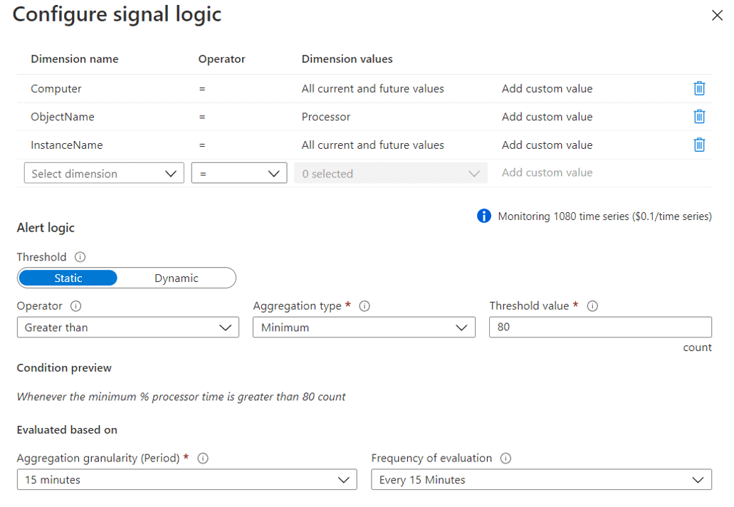
Let’s analyse an example. Imagine you would like to build an alert to notify you everytime a processor core is over 80% for more than 15 minutes. It seems an easy example to use a metric, right?

That’s what happens when you choose to use metrics:

Since the check will be by core, the alert needs 3 dimensions: Computer, the metric (processor) and the instance (core). However, we also can’t overreact. Any core can easily be over 80% at any moment, that’s why we need to configure the 15 minutes of check. The processor will only be in trouble if over 80% during 15 minutes.

The configuration is like this:

Another Option for the Alerts

Log Analytics uses Kusto Query Language, or KQL, to query the information on its storage. Using it we can build a query capable of achive the same result as the monitoring metric. Learn a new query language to build this is not the easier task when starting a migration, but the difference may worth it.

The KQL query we need will be this one:

Perf
| where CounterName==”% Processor Time” and InstanceName != “_Total” and ObjectName==”Processor”
| where TimeGenerated>=ago(15m)
| summarize MinProcesor=min(CounterValue) by Computer,InstanceName
| where MinProcesor >=80

The price difference is amazing:

When we use metric alerts

Such a high price difference would turn metrics useless. Why would anyone use metrics for alerts if KQL is so cheaper?

• Alerts are not exclusive for Log Analytics. Almost every Azure object has the Alerts tab, allowing you to create alerts over them. In these situations, you will not have the option to use KQL.
• using KQL we have two levels of delay: the Log Analytics log collect schedule and the alert check schedule. There may be situations where this delay would not be acceptable

Configuration and Exception

On the objects where we don’t have the Log option to build conditions, we still can use KQL queries instead of metrics. We can configure the objects to send all their log to a log analytics on our azure environment. By doing that, we will be able to configure the alerts for all of them on the log analytics environment.

The objects’ configuration is not in the same place or exactly the same everywhere. Let’s analyse the existing variations.

Data Factory and most of the objects

On most of the objects, the configuration is made using the Diagnostics option under Monitoring, like the image below:

Azure SQL 

On Azure SQL objects, the same configuration is made using the Auditing option under Monitoring, like the image below:

 

Resource Groups

On Resource Groups, using the Diagnostics option, we can manage the diagnostic settings for all the objects inside the resource group. It doesn’t mind if the objects’ configuration are made in different ways, such as Data Factory and Azure SQL objects, they can all be controlled from the resource group.

Clicking on the Enabled or Disabled icon you will see the configuration screen for the object you clicked, so the resource group becomes a central point to manage the diagnostic settings for all the objects in the resource group.

 

Storage Accounts

On storage accounts, there are two monitoring solutions. The monitoring solutions we are talking about is called “classic” on storage accounts, there is a new one for them.

 

 

 

The new monitoring configuration stores all the storage account’s log together the activity log of the object. This allows us the following benefits:

• Use KQL queries over the object
• Create KQL alerts over the object, without using Log Analytics
• Build Workspaces to visualize what’s happening with the storage account

 

 

 

 

The post Saving money with Log Analytics appeared first on Simple Talk.

from Simple Talk https://ift.tt/3mLQVd6
via