Friday, March 12, 2021

Ways to get and deal with invalid node identifiers in SQL Server Edge references

One of the weirder things about graph tables in SQL Server is the mysterious backend implementation. The values you see when working with these objects look like this: {“type”:”node”,”schema”:”dbo”,”table”:”Node1″,”id”:0}, but when you get errors, you don’t see the json, you see what this represents (two integers for the object_id and unique id in the graph table, as I showed in this blog). Since all of this happens in the engine, the values you see in the JSON, you kind of expect would have to correspond to something real. But this is not always the case. There are two ways (that I know of) that this can happen. The first way is when you delete nodes that had edge references but not constraint. The next way is the just insert invalid (or at least, currently invalid data).

For example, take these two node objects, and 2 edges:

CREATE TABLE dbo.Node1(Name varchar(20)) AS NODE;
CREATE TABLE dbo.Node2(Name varchar(20)) AS NODE;

For one edge table, I will create it to allow any nodes to connect:

CREATE TABLE dbo.Edge1 AS EDGE;

And then another edge, but this one will have 2 edge conditions defined to use cascading deletes (so if either node is deleted, the edge is removed).

CREATE TABLE dbo.Edge2
(
        CONSTRAINT EC_Edge2 CONNECTION 
                (dbo.Node2 TO dbo.Node2, 
                 dbo.Node1 TO dbo.Node2) ON DELETE CASCADE
) AS EDGE;

Next I will add a couple of nodes to each node table:

INSERT INTO dbo.Node1(Name)
VALUES('One'),('Two');

INSERT INTO dbo.Node2(Name)
VALUES('Buckle'),('Shoe');

Take a look at the data that has been created:

SELECT *
FROM   dbo.Node1;
SELECT *
FROM   dbo.Node2;

Each row output has the node_id value (with a unique name amongst all other tables.

$node_id_1E3D804E50C142CEA8041BF16862E7AC                Name
-------------------------------------------------------- --------------------
{"type":"node","schema":"dbo","table":"Node1","id":0}    One
{"type":"node","schema":"dbo","table":"Node1","id":1}    Two
$node_id_28039674CFE4498FB0B24CDAD854F145                Name
-------------------------------------------------------- --------------------
{"type":"node","schema":"dbo","table":"Node2","id":0}    Buckle
{"type":"node","schema":"dbo","table":"Node2","id":1}    Shoe

Using those values, we can establish a link in both edges, with the same id values. Edge1:

INSERT INTO dbo.Edge1($from_id, $to_id)
SELECT (SELECT $node_id FROM dbo.Node2 WHERE name = 'Buckle'),
           (SELECT $node_id FROM dbo.Node2 WHERE name = 'Shoe');

INSERT INTO dbo.Edge1($from_id, $to_id)
SELECT (SELECT $node_id FROM dbo.Node1 WHERE name = 'One'),
           (SELECT $node_id FROM dbo.Node2 WHERE name = 'Buckle');

Then edge2:

INSERT INTO dbo.Edge2($from_id, $to_id)
SELECT (SELECT $node_id FROM dbo.Node2 WHERE name = 'Buckle'),
           (SELECT $node_id FROM dbo.Node2 WHERE name = 'Shoe');

INSERT INTO dbo.Edge2($from_id, $to_id)
SELECT (SELECT $node_id FROM dbo.Node1 WHERE name = 'One'),
           (SELECT $node_id FROM dbo.Node2 WHERE name = 'Buckle');

Looking at the data in Edge1:

SELECT Node2.Name AS FromNode, LinkedTo.Name AS ToNode
FROM  dbo.Node2,dbo.Edge1,dbo.Node2 AS LinkedTo
WHERE MATCH(Node2-(Edge1)->LinkedTo);

This returns:

FromNode             ToNode
-------------------- --------------------
Buckle               Shoe

Now we delete a node:

DELETE FROM dbo.Node2
WHERE  Node2.Name = 'Buckle';

Now re-execute the previous query, and you get a seemingly strange result:

FromNode             ToNode
-------------------- --------------------
NULL                 Shoe

If you look at the data in the tables, it is evident what has occurred:

SELECT *
FROM   dbo.Node2;

SELECT *
FROM   dbo.Edge1;

This returns:

$node_id_9163A449BE314C8CAA08E02FF3F1FE3E               Name
------------------------------------------------------- --------------------
{"type":"node","schema":"dbo","table":"Node2","id":1}   Shoe

$edge_id_F8D6E993D86E40A592E94A7E9C08EE99               $from_id_7B55F84E631C4739A4941A6768F1370D              Continued Below
------------------------------------------------------- -------------------------------------------------------
{"type":"edge","schema":"dbo","table":"Edge1","id":0}   {"type":"node","schema":"dbo","table":"Node2","id":0}  
{"type":"edge","schema":"dbo","table":"Edge1","id":1}   {"type":"node","schema":"dbo","table":"Node1","id":0}  
            $to_id_C170E534EA6348B488B4927A955C02CD
            ----------------------------------------------------------
            {"type":"node","schema":"dbo","table":"Node2","id":1}
            {"type":"node","schema":"dbo","table":"Node2","id":0}

You can see in the $from_id and $to_id that there is an id:0 that doesn’t exist in the table. If you do this with the other edge, you will see that because of the CASCADE connection, that the edge is removed. Neither of the following query returns data:

SELECT Node2.Name AS FromNode, LinkedTo.Name AS ToNode
FROM  dbo.Node2,dbo.Edge2,dbo.Node2 AS LinkedTo
WHERE MATCH(Node2-(Edge2)->LinkedTo);

SELECT *
FROM   dbo.Edge2;

Going back to the Edge1 object, we are missing the Buckle node, but if you try to add it back:

INSERT INTO dbo.Node2(Name)
VALUES('Buckle');

But even after you add back the row, the orphaned key value in the $from_id and $to_id values is not added so the following query still returns NULL for the Buckle side of the result:

SELECT Node2.Name AS FromNode, LinkedTo.Name AS ToNode
FROM  dbo.Node2,dbo.Edge1,dbo.Node2 AS LinkedTo
WHERE MATCH(Node2-(Edge1)->LinkedTo);

If you want to add back that data in exactly the form it came as, you have to actually create that value manually by providing the node_id to the insert, using the format that you get from the output of the queries:

DELETE FROM dbo.Node2 WHERE Name = 'Buckle';

INSERT INTO dbo.Node2($Node_id, Name)
VALUES ('{"type":"node","schema":"dbo","table":"Node2","id":0}','Buckle')

Now you see the following:

SELECT *
FROM   dbo.Node2;

This returns:

$node_id_7AEF81800C7C46808238FA0683232FDA              Name
------------------------------------------------------ -------
{"type":"node","schema":"dbo","table":"Node2","id":0}  Buckle
{"type":"node","schema":"dbo","table":"Node2","id":1}  Shoe

And the MATCH works too:

SELECT Node2.Name AS FromNode, LinkedTo.Name AS ToNode
FROM  dbo.Node2,dbo.Edge1,dbo.Node2 AS LinkedTo
WHERE MATCH(Node2-(Edge1)->LinkedTo);

The row is back:

FromNode             ToNode
-------------------- --------------------
Buckle               Shoe

In a future blog, I will extend this concept of inserting your own nodes and show the value\limitation of the process.

The post Ways to get and deal with invalid node identifiers in SQL Server Edge references appeared first on Simple Talk.


from Simple Talk https://ift.tt/2OmgRjG
via

Thursday, March 11, 2021

What is interpolation?

Interpolation is a mathematical technique which was popular before we had a lot of cheap computing power. The basic idea is that if you’re given a set of data and looking for a value in the same range, you can interpolate it to get a reasonable estimation for the value that is not actually in the set.

If you can find an old calculus, finance, statistics or algebra book, they had lookup tables in the back. Remember that the only computational tools students had back then were pencil and paper or a slide ruler. If you wanted to use a pencil and paper, you had to know what formula to use. If you use the slide ruler, you can only have three decimal places in your answer (yes, there were a couple of over-sized specialized slide rulers which could go as high as four or five decimal places. They were very expensive). But if your slide ruler didn’t have a particular function you were trying to compute, it was hard to get even the three decimal places.

When you try to approximate a value outside the range of your set, that’s called extrapolation. It’s a different topic and requires a slight leap of faith.

Nearest-neighbor interpolation

The nearest neighbor algorithm Is the simplest form of interpolation. It creates a value which is nearest (or equal) to a known value in the table. It does not consider the values of neighboring points at all, yielding a piecewise constant interpolant. This sounds fancy, but it really isn’t. Consider a lookup table for the size of a box for packing an order from a customer, based on the weight or count of the contents. If the items you’re selling are pretty much the same volume per unit of weight in the same shapes, then this might be just fine for your work.

For example, if I own a video store, my packages stand a very good chance of using a limited set of sizes corresponding to the number of DVDs in a shipment. This is because DVDs tend to be close to the same shape and size. The algorithm is straightforward to implement; divide the total number of DVDs in the shipment, pick the smallest boxes that will hold that number of DVDs. For example, if somebody orders 15 discs of “Law & Order”, you can pack it in one 10-unit box and one 5-unit box. This is based on the assumption that these two packages are cheaper than three 5-unit packages which may or may not be true in the real world. Or maybe a 20–unit package with a lot of Styrofoam in it could be the winner. Even worse, it might be possible that sending out 15 single–unit packages is cheaper! Many decades ago, I ran into such a situation when a promotional item was my choice for Christmas gifts. The premium item being offered was already packaged in mailers, so the cost of repacking them would’ve been complicated and prohibitive.

But if I am a general merchandise store, I’m not going to get a fishing pole into the same box that I used for a pair of shoes of the same weight. I ran into a problem like this decades ago, with a picklist for a mail-order barbecue company. Essentially, each order generated a pick list of the various items which were sent to the shipping department be put in boxes with the appropriate dry ice and insulation. The shipping department had to pick the proper size box to use along with the amount of dry ice needed. A bad guess could mean that an order had to be unpacked, put in a new box, and reprocessed. Since much of their Christmas rush was done by temporary help, who lacked the experience to make a good guess, this was getting to be very costly. The first approach their consultant had taken was essentially to play three dimensional Tetris with the items. Ugh!

We found a better approach was to go back to historical data and figure out how many unique orders had been placed in the last several years. As it turned out, we only had 5000 unique configurations on the pick lists. Then within each of the configurations, we picked the smallest box that had been used for shipment and built a lookup table. This became a simple matter of an exact relational division, and a special case (“pack this order by hand”) when the relational division failed.

This challenge is called “bin packing” and “knapsack problems” which is a popular topic in computer science. Generally speaking, there is no guaranteed optimal result.

Linear interpolation

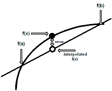
This technique is a way of guessing the results of a function that lies between two known values. Let’s call the two known functional values, a and b, and their results from the function, f(a) and f(b) and try to find f(x), where (a <= x <= b), but x is not in the table. We have to make many assumptions about the function. It has to be continuous over the interval [a, b] and behave smoothly. Thank goodness, most other common functions do behave nicely. It is based on the idea that a straight line is drawn between two function values f(a) and f(b) will approximate the function well enough that you can take a proportional increment of x relative to (a, b) and get a usable answer for f(x).

For example, Let’s assume we have a table of census figures for the years 1970, 1980, 1990 and 2000, and we want to estimate the population for the years 1975, 1985 and 1995. Assume that population growth between the years we know was linear and hope that there were no spikes in births or plagues in between. This method was used by Babylonian astronomers and by the Greek astronomer and mathematician, Hipparchus (2nd century BCE). The algebra looks like this:

f(x) ≈ f(a) + (x - a) * ((f(b) - f(a))/(b-a))

This can be translated into SQL as simple algebra.

DROP TABLE IF EXISTS dbo.SomeFunction
 CREATE TABLE SomeFunction([param] INT, answer INT)
 INSERT INTO dbo.SomeFunction
 (
    [param],answer
 )
 VALUES(1970,3000),(1980,3200),(1990,3100),(2000,2900);
 
 DECLARE @my_parameter INT = 1975;
 SELECT @my_parameter AS my_input,
 (F1.answer + (@my_parameter - F1.param)
 * ((F2.answer - F1.answer)
 / (CASE WHEN F1.param = F2.param
 THEN 1.00
 ELSE F2.param - F1.param END)))
 AS answer
 FROM SomeFunction AS F1, SomeFunction AS F2
 WHERE F1.param -- establish a and f(a)
 = (SELECT MAX(param)
 FROM SomeFunction
 WHERE param <= @my_parameter)
 AND F2.param -- establish b and f(b)
 = (SELECT MIN(param)
 FROM SomeFunction
 WHERE param >= @my_parameter);

The CASE expression in the divisor is to avoid division by zero errors when f(x) is actually in the table, and we are only looking at one point.

linear interpolation

Nonlinear interpolation

Linear interpolation assumes a well-behaved function, which grows in a linear fashion. It is quite possible that something may have rapidly increasing growth. Consider a table of a population census for the years 1960, 1970, 1980 and 1990. This model assumes the population for the year 1975 should be halfway between 1970 and 1980. But the truth might be that there was a period of really rapid population growth in the late 1970s because of massive immigration, an increase in birth rate, or other factors. Likewise, we could have massive population decay due to a plague, famine, war, or other events. You can actually see this pattern in the parish records of England. With the rise of capitalism, a population that had been in a “sawtooth pattern” for centuries suddenly changed to uninterrupted growth. It wasn’t that people began to breed like rabbits, but they stopped dying like flies.

Common forms of nonlinear data are growth and decay. Simple linear interpolation assumes that the steps within [a, b] are uniform. But growth would assume that as we seek a missing value closer to b, the value of f(x) Increases more rapidly. Now we’re dealing with first derivatives and a little bit a calculus. Those old books I’ve mentioned with the lookup tables also included a value called the first Delta and the second Delta. It was usually a simple formula that added a “fudge factor” to the simple linear interpolation.

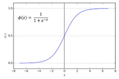
Another common form of nonlinear data is the sigmoid, “S-shape” or Logistics function. If you’ve ever followed a fad, you have seen this sort of data; it starts slow, gains momentum, grows to an inflection or saturation point and then gradually flattens out over time. Consider the sales of incandescent light bulbs, which were replaced by mercury vapor bulbs (“corkscrew lights”) and currently by LED light bulbs. The trick with such growth and decay patterns is predicting where the inflection point is and how long It will take the new technology to replace the prior technology. Failure to do this can leave you with a lot of eight-track cassettes, bell-bottom pants and an unreturnable inventory.

non-linear interpolation

Another form of interpolation is to use polynomials to approximate functions whose computations would otherwise be too complicated. These polynomial approximations are only good over a certain range, and the function for the error is also known. To give an example, log10(x) can be approximated over the range 1/√10 to √10 by the polynomial:

log10(x) ≈ 0.86304 ((x -1)/(x +1)) 
   + 0.36415 ((x -1)/(x +1))3

There are several kinds of polynomials that can be used this way. One of the most common is the Chebyshev (also transliterated as Tchebychev) polynomials.

Conclusion

In fairness, given that modern software has pretty good libraries for functions, you’re probably not going to do a lot of floating point arithmetic from scratch. In fact, given that most of you will be doing commercial rather than scientific work, you probably will do most of your computations with decimal data types and will follow legal requirements that governments, auditors and accountants (EU requirements and GAAP rules) have set up for you. But I still feel, however, it’s good to know such things exist, in case you ever have to go to a reference book and figure out what’s going on. Even if a professional doesn’t use them very often, a professional ought to know what they are and where to find them.

References

Cody, W. J. (1970). “A Su.rvey of Practical Rational and Polynomial Approximation of Functions”. siam Review. 12 (3): 400–423. doi:10.1137/1012082

Hart, John F. (1978). “Computer Approximations:SIAM series in applied mathematics”.ISBN 0–8827–642–7

Martello, Silvano and Toth Paolo.  “Knapsack Problems: Algorithms and Computer Implementations” by (ISBN 0–471–92420–2). The book is old, a bit heavy on math, and the computer code given the back is in FORTRAN. But the text uses an Algol family pseudo-code that should be fairly easy for anyone to read and turn into a modern procedural language. You can download it at http://www.math.nsc.ru/LBRT/k5/knapsack_problems.pdf.

RAND Corporation.  “Approximations for Digital Computers”  (1955).  This has been reprinted as a classic ISBN 978-0691653105. You might remember the RAND Corporation as the people that gave you a table of a million random digits (also still in print).


The post What is interpolation? appeared first on Simple Talk.


from Simple Talk https://ift.tt/3rE4BcU
via

Monday, March 8, 2021

The Game Changed: Power BI Premium per User

Until now, one common knowledge about Power BI was how Power BI Premium subscription is expensive. We, regular mortals, could only dream with the full set of features offered by Power BI Premium.

The new announcement is a complete game changing for the enterprise self-service BI technology: Power BI Premium per User will be available on April 2nd . It will cost only additional us$10,00/month for the users who already have the PRO subscription.

Let’s review what great features we will have available once we subscribe for the Premium per user:


Conclusion

Everyday Power BI gets more features, proving why Microsoft is a leader on Gartner Quadrant. The Power BI Premium per user is more than a simple new feature, is a totally gaming change news, because it brings very powerful features to small and medium size companies.


The post The Game Changed: Power BI Premium per User appeared first on Simple Talk.


from Simple Talk https://ift.tt/3el7340
via

Friday, March 5, 2021

Translating Index/Key Errors from Graph Tables in SQL Server

As I am working with graph tables, I find some quirks exist that make them interesting to work with. One of them is how the values show up in some error messages (in particular from unique indexes). Instead of the details you expect\hope (Something like the JSON value you find in the id columns in the edge and node tables like: {“type”:”node”,”schema”:”dbo”,”table”:”Node”,”id”:0}), you get a pair of numbers that you need to decode.

For example, take the following set of tables:

CREATE TABLE dbo.Node(Name varchar(20)) AS NODE;
CREATE TABLE dbo.Edge AS EDGE;

ALTER TABLE dbo.Edge ADD CONSTRAINT AKEdge UNIQUE($from_id, $to_id);

INSERT INTO dbo.Node (Name) VALUES ('Fred');
INSERT INTO dbo.Node (Name) VALUES ('Barney');

INSERT INTO dbo.Edge ($From_id, $to_id)
SELECT  (SELECT $node_id FROM dbo.Node WHERE name = 'Fred'),
                (SELECT $node_id FROM dbo.Node WHERE name = 'Barney');

Now, insert a duplicate node using the same code as the previous:

INSERT INTO dbo.Edge ($From_id, $to_id)
SELECT  (SELECT $node_id FROM dbo.Node WHERE name = 'Fred'),
                (SELECT $node_id FROM dbo.Node WHERE name = 'Barney')

This causes the following error message:

Msg 2627, Level 14, State 1, Line 14
Violation of UNIQUE KEY constraint 'AKEdge'. Cannot insert duplicate key 
in object 'dbo.Edge'. The duplicate key value is (455672671, 0, 455672671, 1).

So what is this: (455672671, 0, 455672671, 1)? If you look at the $node_id value from the following query:

SELECT $node_id FROM dbo.Node WHERE name = 'Fred';

This returns:

$node_id_F1ECB5498FC747CFBC24EF390EBCBCC9
---------------------------------------------------------
{"type":"node","schema":"dbo","table":"Node","id":0}

The 0 for the id maps to the 0 in the error message (455672671, 0, 455672671, 1), and if you check the row for Barney, you will see that it has a 1 for the id.

But what about the other number? This is the object_id for the table. You can see in this sample data it is duplicated but they could be different, but that value can be different (and will be for things like edge constraints where you are disallowing connection from two different node types in an edge.)

To see this, execute:

SELECT OBJECT_SCHEMA_NAME(object_id) AS schema_name, name AS ObjectName
FROM   sys.tables
WHERE  tables.object_id = 455672671

This returns:

schema_name      ObjectName
---------------- --------------------------
dbo              Node

To make this whole process a little easier, I created the following function (download here: https://github.com/drsqlgithub/DRSQL_ORG-Uploads/blob/main/Tools/ in a file named GraphError.sql):

CREATE OR ALTER PROCEDURE Tools.GraphDB$LookupItem
(
        @ObjectId int,
        @Id int 
)
AS
BEGIN
        SET NOCOUNT ON;
        DECLARE @SchemaName sysname = OBJECT_SCHEMA_NAME(@ObjectId),
                    @TableName sysname = OBJECT_NAME(@ObjectId),
                @SQLStatement nvarchar(MAX)
        SET @SQLStatement = CONCAT('SELECT * FROM ', 
            QUOTENAME(@SchemaName),'.',QUOTENAME(@TableName),
            ' WHERE JSON_VALUE(CAST($node_id AS nvarchar(1000)),''$.id'') = ',@Id)
        EXECUTE (@SQLStatement)
END;

Using this, you can simply paste the values from the error message and execute the stored procedure to see the row that is offending. Execute this next query and get the two rows that represent the errored row, without knowing what table the object is from:

EXEC Tools.GraphDB$LookupItem 455672671, 0;
EXEC Tools.GraphDB$LookupItem 455672671, 1;

This returns:

$node_id_F1ECB5498FC747CFBC24EF390EBCBCC9                Name
-------------------------------------------------------- --------------------
{"type":"node","schema":"dbo","table":"Node","id":0}     Fred

$node_id_F1ECB5498FC747CFBC24EF390EBCBCC9                Name
-------------------------------------------------------- --------------------
{"type":"node","schema":"dbo","table":"Node","id":1}     Barney

I kept the code simple and just returned all columns, but it could easily be extended for whatever you need with a few additional tables of metadata…With a little work you could use the metadata from the objects related to the errored object and produce cleaner output… Something I may attempt later.


The post Translating Index/Key Errors from Graph Tables in SQL Server appeared first on Simple Talk.


from Simple Talk https://ift.tt/2MTNAMM
via

How SQL Server synonyms help database DevOps

Synonyms inside SQL Server are one of those useful but forgotten features. A synonym is a database level object that allows you to provide an alternative name for another database object such as a view, user defined table, scalar function, stored procedure, inline table valued function (tvf), or extended stored procedure. They can also be used for CLR Assembly related stored procedures, CLR tvf, CLR scalar functions or even CLR aggregate functions. There are many practical uses for synonyms, and I’ll explain how to create them and some use cases.

You can create a synonym using the GUI in SSMS or via a script. Here’s a sample script:

USE [AdventureWorks2014]
GO
CREATE SYNONYM [dbo].[EmployeeDemo] 
FOR [MRSurfacePro].[AdventureWorks2014].[HumanResources].[Employee]
GO

The example creates an alternate name for the HumanResources.Employee table. Note that creating the synonym requires a four-part name, including the server. Here’s an example of how to use the new synonym:

SELECT * from dbo.[EmployeeDemo]

If you also query the original table, you’ll see that it returns the same rows. You can reference the new name in code, linked servers, applications, and more. In situations where you would need to use a three- or four-part name, you can just use the synonym without having to use the multipart naming which greatly reduces the need for code changes.

There are a few caveats to this to keep in mind. Synonyms cannot be referenced things like CHECK constraints, computed columns, default expressions, rules expressions, schema bound views or functions. They also cannot be used in DDL (Data Definition Language) statements, to make changes to the underlying schema the synonym represents, you must reference the actual object name within any DDL statement.

We all know when developing objects, the naming that was used at the beginning of a project can change and get better over time. Using synonyms can be a real project time saver. You can continue to be agile and not have a huge need to back port changes. Synonyms can also help with database migrations from one server to another. How many times have you had to migrate to a server with a new name? This simplifies the process. All you would have to do is change the synonym definition four-part name; no other changes would be required.

Imagine how easy this can make DevOps. Say you have a cross-database view and database names are different on the development server or servers in the pipeline. If you use synonyms, no additional code changes are needed when referencing the view, and a post-deployment script could just change the synonym definition depending on the environment.

Synonyms simplify and remove the need for code changes. It’s definitely something to consider. I am always cautious as a DBA to recommend things like this as it tends to make it more difficult to track down issues and troubleshoot back to the original table or source, so be sure to document them. There are times, however, in which we need to accomplish things as I explained above, and synonyms are a great avenue to do so.

The post How SQL Server synonyms help database DevOps appeared first on Simple Talk.


from Simple Talk https://ift.tt/3ec9qWW
via

Monday, March 1, 2021

Parameter Sniffing or not sniffing: The Mindset change for new technologies

Parameter sniffing is a common challenge for query tuning. The usual solution we recommend is to apply a recompile option, rather to a stored procedure or a query. If the development team gets used to this, suddenly you will see recompile options all around.

Query Tuning 101

The parameter sniffing problem appears when the data is uneven distributed on one column used as predicate. As a result, the perfect plan for the query will be different according to the value used on the predicate. Applying a recompile option solves the parameter sniffing problem because the query will be recompiled for each set of parameters, ensuring the best query plan possible.

Here are some examples about how the plan can be affected:

  • A pair of headphones Description automatically generated with medium confidence A key lookup can be applied if the number of rows returned is small or an index scan will be applied if the number of rows returned is too big.
  • A join can be made using nested join or hash join, according to the number of rows returned.
  • The memory allocated can become too much, or to low, and if it’s too low, it will cause spills to tempdb and performance problems, and this will be terrible for performance.

In order to ensure the plan will be recompiled on every execution, we have some different options:

  • We can apply the clause ‘With Recompile’ to a stored procedure. It will make the procedure be recompiled on every execution.
  • We can apply the ‘With Recompile’ clause to the ‘Execute’ statement when executing the stored procedure. This will cause the procedure to be recompiled before the execution.
  • We can apply the clause ‘Option (Recompile)’ to a query, even if the query is inside a stored procedure.

However, the solution has a price: We are losing the power of the query plan cache, forcing a recompilation on every execution, what affects performance. We are only choosing the cheaper option.

New Solutions for Parameter Sniffing

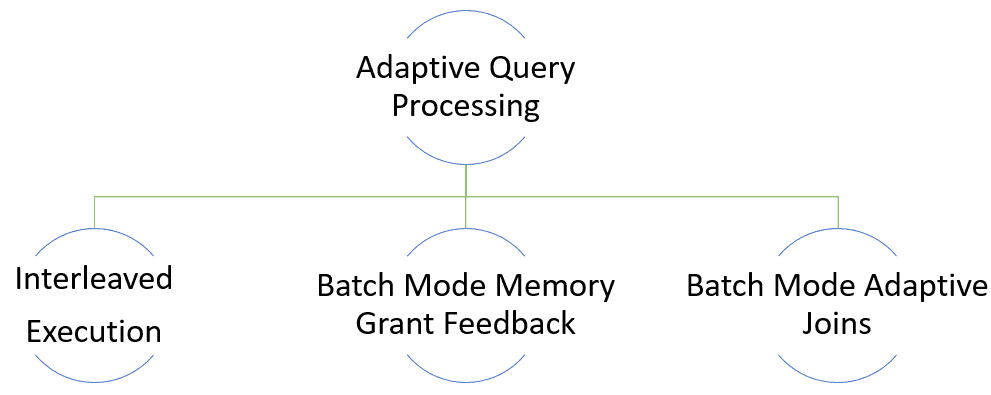
Microsoft is aware of this and SQL Server created many features to help us solve the parameter sniffing problem. These are three of them:

  • Query Store can identify queries suffering with parameter sniffing
  • Memory Grant Feedback can solve some memory allocation problems caused by parameter sniffing
  • Adaptive joins can solve problems with join selection caused by parameter sniffing
  • Batch mode over row store allows adaptive joins to be applied over row mode queries

Diagram, timeline Description automatically generated

That’s great! We can continue solving our problem with the recompile options but now these great new features will jump in and make our queries even better, right?

Wrong!

Memory Grant Feedback and Adaptive Joins are part of the Adaptive Query Processing while Batch mode over row store is part of its big brother, Intelligent Query Processing.

So, what?

Adaptive Query Processing is based on the idea of changing some behaviours of the query plan during the execution, without a new query compilation. This is in some ways the opposite of our traditional solution, the recompile options. We can choose always to recompile the plan or we can use the new Adaptive Query Processing features, but we can’t use both, they will be, at most, useless.

We need to analyse each one of them to understand.

Adaptive Joins

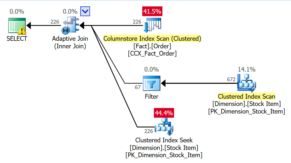
Adaptive Join is a query plan operator capable to create alternate paths inside the execution plan. These alternate paths allow SQL Server to choose the best join option according to the number of rows returned on each execution. In other words, a different behaviour on each execution according to the number of rows returned.

This solution handles the parameter sniffing problem for join selection in a great way: The decision of what type of join will be used is made during each execution, according to the number of rows returned. Parameter sniffing will not affect join type decision anymore.

Diagram Description automatically generated with low confidence

However, if we apply any recompile option, the adaptive join loses its meaning. Each compilation can decide what type of join is best for the plan, there is no need of the adaptive join at all.

Adaptive Joins and Recompiles

This creates some resulting scenarios not so good for us:

  • The widespread use of recompile options will prevent you from enjoying the benefits of this new feature. This means your queries could be better, they could avoid paying the recompile price, but having the recompile mindset spread among developers will prevent deeper analysis.
  • Besides the recompilation price, you will still have the adaptive join in your query plan. Probably the cost is meaningless, but it still creates some extra steps during compilation and execution.
  • There is, indeed, one chance that even using recompilations, the adaptive join will still improve the query. How? The compilations are based on existing statistics, while adaptive join is based on the actual rows during the execution. If the statistics were not updated, the plan without adaptive join could be wrong, while the adaptive join would not be affected (unless the statistics are so bad you end up without the adaptive join at all). This creates a hide-and-seek game: Your performance improved, cool! But it’s hiding the fact it could be better, because you could get rid of the recompilations, that’s bad. It’s also hiding the fact you are not making a good statistics maintenance and that is very bad.
  • Who will fully enjoy the new features without many concerns are exactly the ones who were not taking much care of the query performance and haven’t used recompile options to solve parameter sniffing. The most careful ones will need to deal with mindset change in the DBA and development team leading to many strange scenarios.

Memory Grant Feedback

Parameter sniffing can make the amount of memory needed by one query vary too much. This variation will create spills to tempdb, making the query way slower.

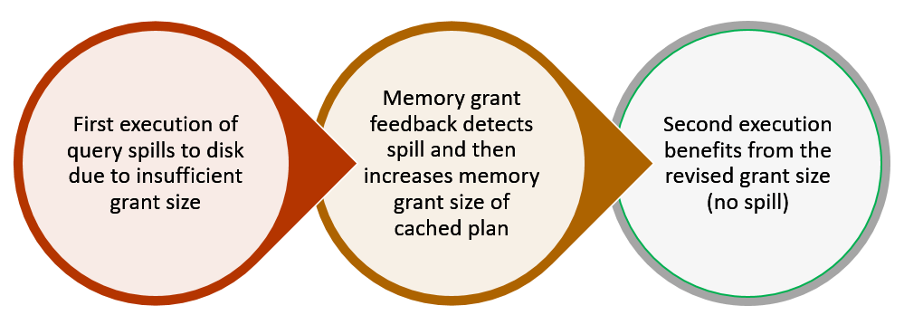
Memory Grant Feedback can solve this problem in some situations. It’s simple: If a difference is found between the memory needed and the memory allocated, this feature changes the query plan directly in the cache for the next execution. As a result, while one execution goes bad with a wrong amount of memory allocated, the next one will be fixed.

Diagram Description automatically generated

The Effect over Sniffing

The effect over parameter sniffing is only partial. Let’s imagine the variation of the parameter values generate two different plans according to the value. If each plan is executed a considerable number of times before a different plan is needed, the Memory Grant Feedback will improve the query.

However, if different plans are needed on a very high frequency, such as on each execution, the Memory Grant Feedback will not be useful. This feature identifies the problem, change the plan and the improvement will happen on the next execution. If the next execution needs a different plan or different set of resources, the change was useless. After 32 useless changes caused by the Memory Grant Feedback, the query optimizer disables this feature for the query plan.

Recompile

The use of recompile option turns the feature completely useless. This feature is based on the same plan executed multiple times. Recompiling the plan on every execution invalidates the feature.

Conclusion

It doesn’t matter how simple new features are, the technology evolves way faster than company and department procedures. In order to fully enjoy new features, you may need some mindset change.


The post Parameter Sniffing or not sniffing: The Mindset change for new technologies appeared first on Simple Talk.


from Simple Talk https://ift.tt/3dUpQDj
via

HOW CAN SQL SERVER DEVELOPERS GET STARTED WITH POSTGRE SQL?

WHAT IS SQL SERVER?

SQL server is a relational database management system. It is offered by Microsoft and is one of the most popular relational database management systems which are being utilized by several companies for their database requirements. There are numerous USPs of Microsoft SQL Server which makes it a popular choice. Some of them include: online analytical processing, data mining, interactive GUI and database performance enhancers and analyzers.

WHAT IS POSTGRE SQL?

PostgreSQL on the other hand is not offered by one specific company but is rather an open-source tool. When a piece of technology falls into the open-source category, it suggests that the code is being read and reviewed by numerous developers around the world. The worldwide developer community is capable of making significant contributions to the open-source projects which automatically increases the chances of quick bug fixes and more enhancements. PostgreSQL is extremely popular in terms of open-source relational database management systems. Developers are attracted to PostgreSQL because there is no fee to use PostgreSQL in its full capacity, it can be integrated with several other languages like C++ and Java and performs all the functionalities that are offered by any paid modern relational database management system.

WHAT CHANGES CAN YOU EXPECT WITH THE GUI?

In SQL server, the views and schemas are displayed in the Microsoft SQL Server Management Studio where the developer is able to see the connections between the relations, observe the structure of the table, write queries and see the output of those queries. In addition to this, SQL Server developers are also used to proper indenting and colored syntax highlighting while running their SQL queries in the studio, getting readymade templates for basic SQL functionalities and statistics regarding the time and the resources utilized when their queries are run.

On the other hand, in PostgreSQL, the views and schemas are displayed in the Data Architect which is the GUI offered by PostgreSQL for developers to visualize the structure and relationship of the entities and relations in their database. The number of tools available in Data Architect might overwhelm a SQL Server developer first but since the basic structure – visualization of schema, query running console, query output window etc. is similar, it won’t be long when the developer starts getting comfortable with PostgreSQL’s GUI.

WHAT VARIATIONS WILL YOU OBSERVE WITH COMMAND LINE UTILITIES?

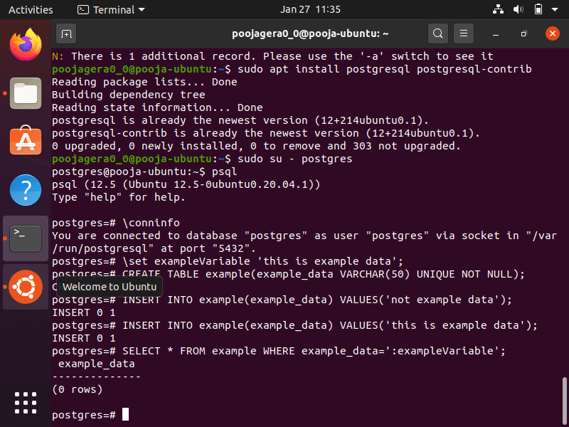
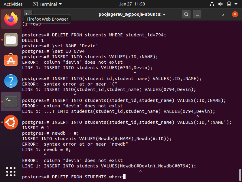
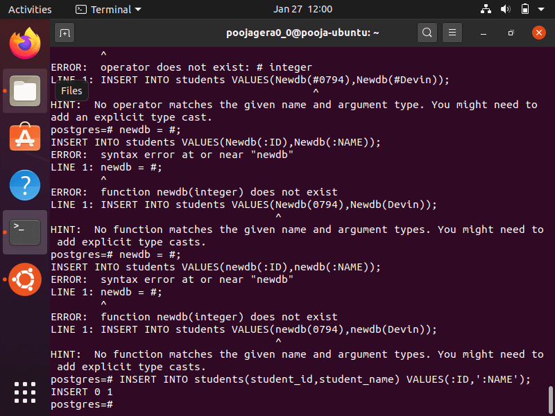
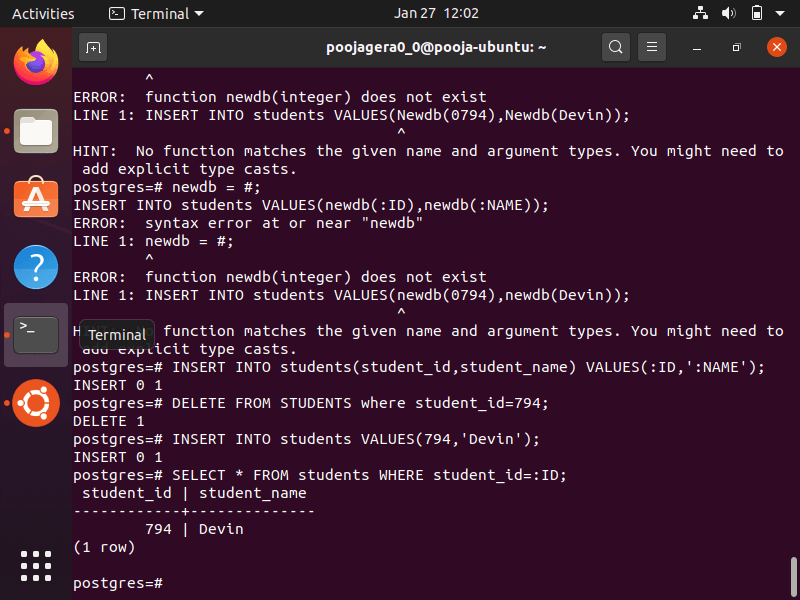
For SQL Server developers sqlcmd utility is no brainer. Similarly, in PostgreSQL psql is the command line utility. Below mentioned are few examples and commands which the developer can perform in PostgreSQL using the psql utility:

  1. Variable Substitutions
    1. Set a variable:
    2. Create a list of variables:
    3. Using the defined variables as data to be inserted in the table:

  1. SQL Interpolation

WHAT CHANGES YOU SHOULD EXPECT IN THE SYNTAX OF SQL QUERIES?

Microsoft SQL Server utilises T-SQL or Transact SQL. T-SQL has all the features and functionalities of a language required for managing databases. It contains DDL, DML, user defined variables, functions and procedures. However, developers are also used to using several relational operators and table expressions while using the SQL Server. PostgreSQL supports all the basic functionalities of entry-level SQL. It was PostgreSQL which contributed in the development of several object-relational features. While PostgreSQL does not have inbuilt OLAP features, being open source, it can easily be connected with external OLAP offering servers.

WHAT VARIATIONS WILL YOU OBSERVE FROM SQL SERVER TO POSTGRESQL TAKING DATATYPES INTO CONSIDERATION?

SQL Server supports the following datatypes:

  1. Basic Datatypes: character, binary string, text, images.
  2. XML Type: This is used to store XML data.
  3. Sql_variant Type: It contains information about SQL scalar types with filter, join and sort functionalities being offered for columns which are of sql_variant datatypes.
  4. Table Type: This is a type which cannot be assigned to a column. This can only be assigned to variables which are being used in the structure. While creating functions and procedures, it is not advisable to use the table directly and hence a table type variable is used for performing various tasks related to a function or a procedure.
  5. Cursor Type: Cursor Type, like Table Type is a datatype which cannot be assigned to columns and can only be assigned to variables. It is used to refer to cursor objects.

On the other hand, you will observe some more advanced (or different) data types when you are starting with PostgreSQL. Make sure you have familiarized yourself with the use cases of these data types to work with them smoothy.

  1. Base Types: These are abstract data types which include basic data types like int, complex etc.
  2. Composite Types: These datatypes are created automatically by PostgreSQL whenever a new table is created. It contains information about the rows of the table. They can be declared by the developer as well.
  3. Domains: Domains are another kind of base types.
  4. Pseudo Types: Pseudo types are data types which cannot be assigned to a column. They can be used either as arguments or function return types.
  5. Polymorphic Types: anyelement and anyarray are two pseudo types which are known as polymorphic types.
  6. Geometric Data Type: This datatype is used to represent 2D shapes on which different in-built geometric functions can be performed.
  7. Storage of network addresses: PostgreSQL also offers a datatype wherein network addresses can be stored. Pretty handy if you are making an application which requires geo-tracking and geolocation services and also has support to perform operations on these addresses.
  8. Bit type: For storage of data in binary and perform operations on it.

TABULAR COMPARISON BETWEEN THE SYNTAX AND FEATURES OF POSTGRE SQL AND MS SQL SERVER FOR REFERENCE

Given below are some common parameters which have been used to draw a comparison between the structural query languages used by both PostgreSQL and MS SQL Server. The rows highlighted in green indicate that there is no difference between the SQL syntax of PostgreSQL and MS SQL Server.

Parameter

PostgreSQL

MS SQL Server

NATURAL JOIN

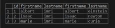
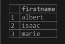
select firstname from scientist natural left join not_scientist;

No support.

USING keyword

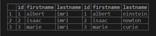
select * from scientist inner join not_scientist using(id);

No support.

FULL JOIN

select * from scientist full join not_scientist on scientist.id = not_scientist.id;

select firstname from scientist full outer join not_scientist on scientist.id=not_scientist.id;

CROSS JOIN / CARTESIAN PRODUCT

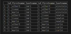
select * from scientist cross join not_scientist;

SELECT item_name FROM items CROSS JOIN market;

COPY TABLE

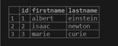
create table copycat_scientist as select * from scientist where false;

insert into copycat_scientist (id, firstname, lastname) values (1, ‘albert’, ‘einstein’);

insert into copycat_scientist (id, firstname, lastname) values (2, ‘isaac’, ‘newton’);

insert into copycat_scientist (id, firstname, lastname) values (3, ‘marie’, ‘curie’);

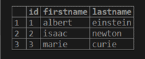
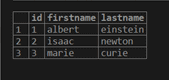
select * from copycat_scientist;

select * into copy_scientist from scientist where 1<>1;

insert into copy_scientist (id, firstname, lastname) values (1, ‘albert’, ‘einstein’);

insert into copy_scientist (id, firstname, lastname) values (2, ‘isaac’, ‘newton’);

insert into copy_scientist (id, firstname, lastname) values (3, ‘marie’, ‘curie’);

select * from copy_scientist;

ORDERING OUTPUT

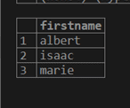
select firstname from scientist order by firstname;

select firstname from not_scientist order by firstname;

LIMIT

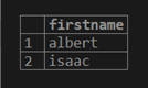
select firstname from scientist order by firstname limit 2;

SELECT TOP 5 item_name FROM items ORDER BY item_id ASC;

INSERT

insert into not_scientist (id, firstname, lastname) values (3, ‘marie’, ‘curie’);


insert into not_scientist (id, firstname, lastname) values (3, ‘marie’, ‘curie’);

BOOLEAN DATATYPE

Supports.

Supports as BIT Datatype

CHAR DATATYPE

Supports.

Supports.

TIMESTAMP

Supports.

Supports but not exactly timestamp, it supports datetime.

CHARACTER_LENGTH FUNCTION

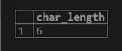
select char_length(‘albert’);

Does not support character length.
Instead:
Len(‘Dior’) and DATALENGTH(‘Dior’s Handbag’) are used.

SUBSTRING

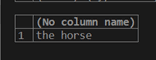
select substring(‘the horse and the grass and the stable’ from 10 for 20);

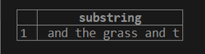
select substring(‘the horse and the grass and the stable’, 0, 10);

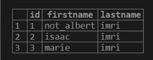
REPLACE

update scientist set firstname = replace(firstname,’albert’,’not_albert’);

select * from scientist;

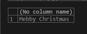
select REPLACE(‘Merry Christmas’,’rr’,’bb’);

TRIM

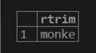
select trim(trailing ‘y’ from ‘monkey’);

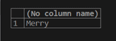
select LTRIM(‘ Merry’);

CONCATENATION

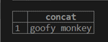
select concat(‘goofy’,’ ‘,’monkey’);

select concat(‘The Goofy’, ‘Monkey’) as nickname;

UNIQUE CONSTRAINT

CREATE TABLE nicknames ( nickname_no integer UNIQUE,

Nickname text

);

CREATE TABLE nicknames ( nickname_no INT UNIQUE,

Nickname VARCHAR(50)

);

TRUNCATE TABLE

TRUNCATE nicknames;

TRUNCATE TABLE nicknames;

CONCLUSION

As a MS SQL Server developer, you already understand the intricacies of databases, relational databases, database management systems and their use cases. The only milestone you have to achieve now is to get familiarized with the GUI of PostgreSQL and practice the commands a bit. Start with a blank slate in your mind keeping in consideration the syntax of the language and since you already are well versed with the conceptual aspect of SQL and RDBMS, you will be able to draw an analogy between both the tools and hence, you will start using PostgreSQL for your applications in no time!

Here are some resources for you to kickstart your journey in learning PostgreSQL:

  1. “The Complete Python/PostgreSQL Course 2.0 by Codestars by Rob Percival, Jose Salvatierra, Teclado by Jose Salvatierra available at Udemy”
    Description: This course will not only walk you through the syntax of PostgreSQL but also guide you in creating 9 real-world projects.
    Language: English
    Link: https://www.udemy.com/course/complete-python-postgresql-database-course/?altsc=781502
  2. “PostgreSQL by FreeCodeCamp”
    Description: FreeCodeCamp is well known for their free and amazingly curated content. This course is a 4 hour, no break, no Ad course which will take you from the basics to advanced with tonnes of examples and practice queries.
    Language: English
    Link: https://www.youtube.com/watch?reload=9&v=qw–VYLpxG4
  3. “PostgreSQL: Advanced SQL Queries by Pinal Dave Available at PluralSight”
    Description: This course contains advanced concepts of PostgreSQL, perfectly suitable for a developer well versed in MS SQL Server.
    Language: English
    Link: https://www.pluralsight.com/courses/postgresql-advanced-sql-queries?clickid=WsGxLk1WsxyLW7fwUx0Mo3QBUkEUMJy9%3AWyb1s0&irgwc=1&mpid=1193463&aid=7010a000001xAKZAA2&utm_medium=digital_affiliate&utm_campaign=1193463&utm_source=impactradius
  4. PostgreSQL Tutorial
    This is an online bible for the explanation of all the commands, concepts and queries.
    Here is the link: https://www.postgresqltutorial.com/
  5. Books
    1. Practical PostgreSQL by O’Reilly
    2. PostgreSQL Up and Running by O’Reilly
    3. Mastering PostgreSQL 12: Advanced Techniques to Build and Administer Scalable and Reliable PostgreSQL Database Applications, 3rd Edition
  6. Official Documentation of PostgreSQL
    There is nothing better than the official documentation to learn about a new piece of technology. It can be hard to go through sometimes, but one thing that is certain is that you will get all the information you need under one hood.
    Link: https://www.postgresql.org/docs/

Happy Learning!


The post HOW CAN SQL SERVER DEVELOPERS GET STARTED WITH POSTGRE SQL? appeared first on Simple Talk.


from Simple Talk https://ift.tt/3uQBS6P
via