Tuesday, March 23, 2021

Mastering TempDB: Managing TempDB growth

The series so far:

  1. Mastering TempDB: The basics
  2. Mastering TempDB: Managing TempDB growth

As you learned in part one of this Mastering TempDB series, TempDB is a global resource used for many operations within SQL Server. You create and allocate temporary user objects such as temporary tables and table variables, rebuild indexes with SORT_IN_TEMPDB=ON, use it for version stores (RCSI), internal objects (worktables, spools, group by, order by) and even DBCC CHECKDB just to name a few. All these operations require space to be allocated in the TempDB database. At times, these operations can result in TempDB growing rapidly, which, in turn, can fill up the file system and cause failures. In this article, you will learn how to fix an overgrown TempDB file that has resulted in it running out of space.

Uncontrolled TempDB growth

There are many reasons for uncontrolled TempDB growth events. Much like your operating system has a page file to handle memory overflows, SQL Server uses TempDB like a page file. The most common occurrence of this is when a query “spills” to TempDB. When you execute a query, the database engine allocates memory to perform join and sort operations. The amount of memory allocated is based on the statistics associated with the columns and indexes. If the estimate is incorrect and the engine does not allocate enough memory, those joins and sorts will spill to disk—which consumes a lot of TempDB resources. Spilling is only one use of TempDB; some of the other ways SQL Server uses this database include storing large temporary tables. Temp tables can lead to uncontrolled growth if they are being populated by a query that needs to be tuned. You could have an Availability Group replica, which runs in snapshot isolation mode, go down, which causes the version store to fill up. You can have a normal workload cause TempDB to have an auto-growth that causes you to run out of drive space. There are countless explanations as to why TempDB can grow. The key administrative task is not only trying to get the drive space back and the system running, but also identifying the cause of the growth event to prevent recurrence.

As a reminder from the first article, you can easily peek inside your TempDB database to see what has caused the file to fill up. These great queries below provided in TempDB msdocs is a good place to start. Once you locate the culprit, you can tune accordingly to prevent the issue from reoccurring.

-- Determining the amount of free space in tempdb
SELECT SUM(unallocated_extent_page_count) AS [free pages],
  (SUM(unallocated_extent_page_count)*1.0/128) AS [free space in MB]
FROM sys.dm_db_file_space_usage;
-- Determining the amount of space used by the version store
SELECT SUM(version_store_reserved_page_count) 
   AS [version store pages used],
  (SUM(version_store_reserved_page_count)*1.0/128) 
   AS [version store space in MB]
FROM sys.dm_db_file_space_usage;
-- Determining the amount of space used by internal objects
SELECT SUM(internal_object_reserved_page_count) 
   AS [internal object pages used],
  (SUM(internal_object_reserved_page_count)*1.0/128) 
   AS [internal object space in MB]
FROM sys.dm_db_file_space_usage;
-- Determining the amount of space used by user objects
SELECT SUM(user_object_reserved_page_count) 
   AS [user object pages used],
  (SUM(user_object_reserved_page_count)*1.0/128) 
   AS [user object space in MB]
FROM sys.dm_db_file_space_usage;

If you use SQL Monitor, you can also view what’s going on in the new tempdb section.
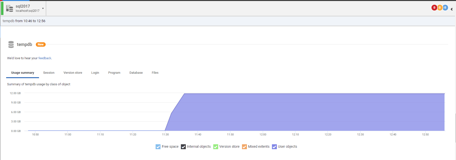
SQL Monitor shows tempdb growth

The following script is my go-to that I have used for years to reactively and proactively understand what’s going on inside TempDB. It was adapted from Microsoft by Kendra Little (B|T) back in 2009 and is still an excellent tool for analyzing TempDB workloads. This script’s query results allow you to clearly identify what space is allocated by a transaction and even capture the query text and its execution plan associated with it.

SELECT t1.session_id,
       t1.request_id,
       task_alloc_GB = CAST((t1.task_alloc_pages * 8. / 1024. / 1024.) 
         AS NUMERIC(10, 1)),
       task_dealloc_GB = CAST((t1.task_dealloc_pages * 
          8. / 1024. / 1024.) 
         AS NUMERIC(10, 1)),
       host = CASE
                  WHEN t1.session_id <= 50 THEN
                      'SYS'
                  ELSE
                      s1.host_name
              END,
       s1.login_name,
       s1.status,
       s1.last_request_start_time,
       s1.last_request_end_time,
       s1.row_count,
       s1.transaction_isolation_level,
       query_text = COALESCE(
                    (
                  SELECT SUBSTRING(
                    text,
                    t2.statement_start_offset / 2 + 1,
                    (CASE
                     WHEN statement_end_offset = -1 THEN
                        LEN(CONVERT(NVARCHAR(MAX), text)) * 2
                     ELSE
                        statement_end_offset
                     END - t2.statement_start_offset
                                            ) / 2
                                        )
                        FROM sys.dm_exec_sql_text(t2.sql_handle)
                    ),
                    'Not currently executing'
                            ),
       query_plan =
       (
           SELECT query_plan FROM sys.dm_exec_query_plan(t2.plan_handle)
       )
FROM
(
    SELECT session_id,
           request_id,
           task_alloc_pages = SUM(internal_objects_alloc_page_count 
               + user_objects_alloc_page_count),
           task_dealloc_pages = SUM(internal_objects_dealloc_page_count 
                + user_objects_dealloc_page_count)
    FROM sys.dm_db_task_space_usage
    GROUP BY session_id,
             request_id
) AS t1
    LEFT JOIN sys.dm_exec_requests AS t2
        ON t1.session_id = t2.session_id
           AND t1.request_id = t2.request_id
    LEFT JOIN sys.dm_exec_sessions AS s1
        ON t1.session_id = s1.session_id
-- ignore system unless you suspect there's a problem there
WHERE t1.session_id > 50 
 -- ignore this request itself 
AND t1.session_id <> @@SPID
ORDER BY t1.task_alloc_pages DESC; 
GO

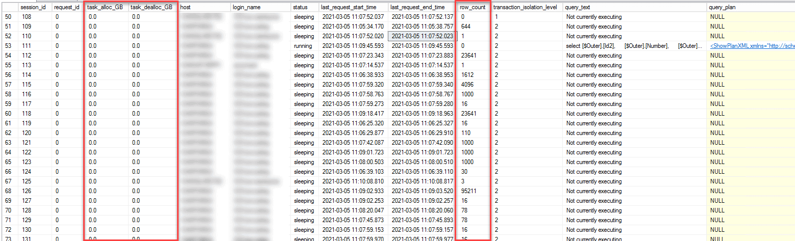
Here are a couple screenshots of the output.

This one shows active row counts, but there is not a ton of space allocated.
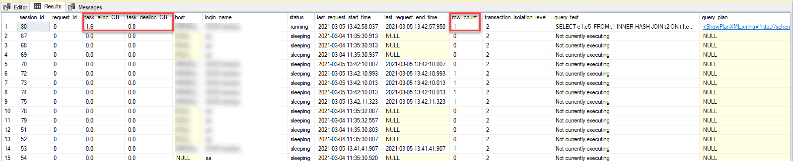
This one shows only one row as a row_count, but look at the task_alloc_GB column. Even though it is only one row, this transaction is taking 1.6GB of space.
Once you identify the culprit, you can move on to resizing. I highly advise you to pause and look at the causal factors before trying to resize, since it is possible to lose all purview to that information. Many of these commands are destructive and will cause you to lose metadata associated with your TempDB growth–this means it is important to capture.

Resizing TempDB

Occasionally, we must resize or realign our TempDB log file (.ldf) or data files (.mdf or .ndf) due to a growth event that forces the file size out of whack. To resize TempDB we have three options, restart the SQL Server service, add additional files, or shrink the current file. We most likely have all been faced with runaway log files, and, in an emergency situation, restarting the SQL Services may not be an option, but we still need to get our log file size smaller before we run out of disk space, for example.

Restart SQL Server Services– since TempDB is non-durable, it is recreated upon service restart at the file size and count that are defined in the sys.master_files catalog view.

Add File– You can quickly get out of trouble by adding another TempDB.mdf file to another drive that has space. This will buy you some time but should be removed once the issue is resolved and your services can be restarted. I only use this one in a true emergency. If you add a file you should plan a restart of your SQL Services because it will now be the most free space file, and your workload will funnel here. So be sure to balance them by restarting to ensure the most efficient round robin use.

Shrink Files– This removes unused space and resizes the file. I’ll explain this process below.

The process of shrinking a datafile can get tricky, so I created this flow chart to help you out if you ever get into this situation. It’s very important to note that many of these commands will clear your cache and will greatly impact your server performance as it warms cache back up. In addition, you should not shrink your database data or log file unless absolutely necessary, but doing so can result in a corrupt tempdb.

Let’s walk through it, and I’ll explain some things as we go along.
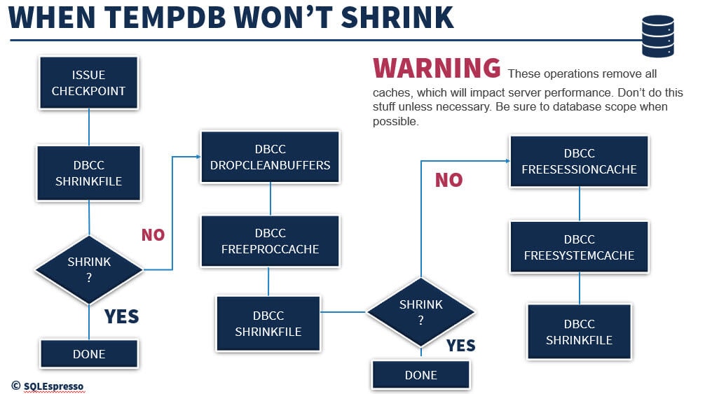
tempdb growth shrinking diagram

First thing you must do is issue a Checkpoint. A checkpoint marks the log as a “good up to here” point of reference. It lets the SQL Server Database Engine know it can start applying changes contained in the log during recovery after this point if an unexpected shutdown or crash occurs. Anything prior to the checkpoint is what I like to call “Hardened”. This means all the dirty pages in memory have been written to disk, specifically to the .mdf and .ndf files. So, it is important to make that mark in the log before you proceed. While TempDB is recreated and not recovered during a restart, however, this is still a requirement of this process.

USE TEMPDB;  
GO  
CHECKPOINT;

Next, we try to shrink the log and data files by issuing DBCC SHRINKFILE commands. This is the step that frees the unallocated space from the database file if there is any unallocated space available. You will note the Shrink? decision block in the diagram after this step. It is possible that there is no unallocated space, and you will need to move further along the path to free some up and try again.

USE TEMPDB;  
GO 
DBCC SHRINKFILE (templog, 1024);   --Shrinks it to 1GB
DBCC SHIRNKFILE (tempdev, 1024);

If the database shrinks, great, congratulations! However, some of us might still have work to do. Next up is to try to free up some of that allocated space by running DBCC DROPCLEANBUFFERS and DBCC FREEPROCCACHE.

DBCC DROPCLEANBUFFERS – Clears the clean buffers from the buffer pool and columnstore object pool. This command will flush cached indexes and data pages.

DBCC DROPCLEANBUFFERS WITH NO_INFOMSGS;

DBCC FREEPROCCACHE – Clears the procedure cache. You are probably familiar with as a performance tuning tool in development. It will clean out all your execution plans from cache, which may free up some space in TempDB. This will create a performance issue as your execution plans now have to make it back into cache on their next execution and not benefit from plan reuse.  It’s not really clear why this works, so I asked TempDB expert Pam Lahoud (B|T) for clarification as to why this has anything to do with TempDB. Both of us are diving into this to understand exactly why this works. I believe it to be related to TempDB using cached objects and memory objects associated with stored procedures which can have latches and locks on them that need to be released by running this. Check back for further clarification, as I’ll be updating this as I find out more.

DBCC FREEPROCCACHE WITH NO_INFOMSGS;

Once these two commands have been run and you have attempted to free up some space, you can now try the DBCC SHRINKFILE command again. For most, this should make the shrink possible, and you will be good to go.  Unfortunately, a few more of us may have to take a couple more steps through to get to that point.

When I have no other choice to get my log file smaller I run the last two commands in the process. These should do the trick and get the log to shrink.

DBCC FREESESSIONCACHE– This command will flush any distributed query connection cache, meaning queries that are between two or more servers.

DBCC FREESESSIONCACHE WITH NO_INFOMSGS;

DBCC FREESYSTEMCACHE – This command will release all unused remaining cache entries from all cache stores, including temp table cache. This covers any temp table or table variables remaining in cache that need to be released.

DBCC FREESYSTEMCACHE ('ALL');

Manage TempDB growth

In my early days as a database administrator, I would have loved to have this diagram. Having some quick steps during stressful situations such as TempDB’s log file filling up on me would have been a huge help. Hopefully, someone will find this handy and be able to use it to take away a little of their stress.

Remember, it is important for you to become familiar with how your TempDB is used, tune those queries that are large consumers and know how to properly resize TempDB if it becomes full.


The post Mastering TempDB: Managing TempDB growth appeared first on Simple Talk.


from Simple Talk https://ift.tt/2Pf6pea
via

Saturday, March 20, 2021

Determining actions you can take with Edge and Node tables in SQL Server

One of the interesting things about working with many-to-many relationships in SQL Server with graph tables instead of a relational table is that unlike a relational many-to-many table, by default an edge may can implement relationships from lots of different tables (nodes). You can also limit what nodes can be related using which edges.

For example, say you have 4 nodes and 2 edges, both of the edges, by default, each edge would allow relationships from each node to itself, or each node to each other node. It can all get a bit complicated to figure out if you have a lot of objects (and to be fair, you probably also want to be able to check to make sure your objects are configured as you expect.

In this blog, I will demonstrate how to determine, given a given edge or node, what operations are possible. To demonstrate, I will use the following nodes and edges:

CREATE TABLE dbo.Node1(Name varchar(20)) AS NODE;
CREATE TABLE dbo.Node2(Name varchar(20)) AS NODE;
CREATE TABLE dbo.Node3(Name varchar(20)) AS NODE;
CREATE TABLE dbo.Node4(Name varchar(20)) AS NODE;

For one edge table, I will create it to allow any nodes to connect:

CREATE TABLE dbo.Edge1 AS EDGE;

And then another edge, but this one will have 2 conditions that are defined to allow cascading deletes (so if either node is deleted, the edge is removed), and one that is requires you to remove the edge to remove the node.

CREATE TABLE dbo.Edge2
(
        CONSTRAINT EC_Edge2 CONNECTION (dbo.Node1 TO dbo.Node2,
                                        dbo.Node2 TO dbo.Node2) 
                         ON DELETE CASCADE
) AS EDGE;
CREATE TABLE dbo.Edge3
(
   CONSTRAINT EC_Edge3 CONNECTION (dbo.Node1 TO dbo.Node2,
                                   dbo.Node2 TO dbo.Node3,
                                   dbo.Node2 TO dbo.Node1) 
                      ON DELETE NO ACTION
) AS EDGE;

To find the metadata about these objects, we can use a couple of base catalog views. sys.edge_constraints and sys.edge_constraint_clauses. sys.edge_constraints is the typical extension of sys.objects, with one row per edge constraint (which is itself an object, like other constraints.) sys.edge_constraint_clauses gives you one row per the node to node relationship. (Note, the query allows for the case where you have more than one edge connection, though that is not generally something you should generally implement (Covered in this blog).

I want to have two views of the metadata, one in the context of the node (what edges exist that I can insert into?) and from the context of the edge (what nodes can be involved in a relationship with the edge?)

So, here first is the query of sys.edge_constraints, showing the constraints that exist:

SELECT object_id AS edge_object_id,
   CONCAT(QUOTENAME(OBJECT_SCHEMA_NAME(
                    edge_constraints.parent_object_id)),'.',
    QUOTENAME(OBJECT_NAME(edge_constraints.parent_object_id))) 
                                                AS ObjectName,
    QUOTENAME(name) AS EdgeConstraintName, 
    delete_referential_action_desc AS DeleteAction
FROM  sys.edge_constraints;

This returns the constraints and what happens on delete:

edge_object_id ObjectName       EdgeConstraintName    DeleteAction
-------------- ---------------- --------------------- ----------------
725577623      [dbo].[Edge2]    [EC_Edge2]            CASCADE
789577851      [dbo].[Edge3]    [EC_Edge3]            NO ACTION

Next to get the nodes that can be involved in the relationship, use:

SELECT object_id AS edge_object_id, 
           CONCAT(QUOTENAME(OBJECT_SCHEMA_NAME(from_object_id)), 
                  '.',QUOTENAME(OBJECT_NAME(from_object_id))) 
                                                  AS FromNode,
           from_object_id,
           CONCAT(QUOTENAME(OBJECT_SCHEMA_NAME(to_object_id)), 
                  '.',QUOTENAME(OBJECT_NAME(to_object_id))) 
                                                  AS ToNode,
           to_object_id
FROM   sys.edge_constraint_clauses;

This returns (less the from and to object_id values):

edge_object_id FromNode         from_object_id ToNode         to_object_id
-------------- ---------------- -------------- -------------- ------------
757577737      [dbo].[Node2]    645577338      [dbo].[Node1]  629577281
725577623      [dbo].[Node1]    629577281      [dbo].[Node2]  645577338
725577623      [dbo].[Node2]    645577338      [dbo].[Node2]  645577338
757577737      [dbo].[Node1]    629577281      [dbo].[Node2]  645577338
757577737      [dbo].[Node2]    645577338      [dbo].[Node3]  661577395

Now I am going to put these together to get the conditions and the constraints:

WITH Constraints AS (
SELECT object_id AS edge_object_id,
           CONCAT(QUOTENAME(OBJECT_SCHEMA_NAME(edge_constraints.parent_object_id)), 
                  '.',QUOTENAME(OBJECT_NAME(edge_constraints.parent_object_id))) AS ObjectName,
           QUOTENAME(name) AS EdgeConstraintName, 
           delete_referential_action_desc AS DeleteAction
FROM  sys.edge_constraints),
Clauses AS (
SELECT object_id AS edge_object_id, 
       CONCAT(QUOTENAME(OBJECT_SCHEMA_NAME(from_object_id)), '.',
              QUOTENAME(OBJECT_NAME(from_object_id))) AS FromNode,
       from_object_id,
       CONCAT(QUOTENAME(OBJECT_SCHEMA_NAME(to_object_id)), '.',
              QUOTENAME(OBJECT_NAME(to_object_id))) AS ToNode,
       to_object_id
FROM   sys.edge_constraint_clauses)
SELECT Constraints.ObjectName, Constraints.EdgeConstraintName, Constraints.DeleteAction, 
       Clauses.FromNode, Clauses.ToNode
FROM   constraints
                JOIN Clauses
                        ON Clauses.edge_object_id = Constraints.edge_object_id;

Thie returns the rough output:

ObjectName     EdgeConstraintName   DeleteAction  FromNode        ToNode
-------------- -------------------- ------------- --------------- -----------------
[dbo].[Edge2]  [EC_Edge2]           CASCADE       [dbo].[Node2]   [dbo].[Node2]
[dbo].[Edge2]  [EC_Edge2]           CASCADE       [dbo].[Node1]   [dbo].[Node2]
[dbo].[Edge3]  [EC_Edge3]           NO_ACTION     [dbo].[Node1]   [dbo].[Node2]
[dbo].[Edge3]  [EC_Edge3]           NO_ACTION     [dbo].[Node2]   [dbo].[Node3]
[dbo].[Edge3]  [EC_Edge3]           NO_ACTION     [dbo].[Node2]   [dbo].[Node1]

In this next query (which is the query I was targeting in the first place), I am going to output an edge centric view, partitioned by object, constraint, giving the delete action and the list of node to node relationships. For edges without an edge constraint, I will use Any Node -> Any Node, rather than listing out every possible permutation of nodes that exist (which would make for a very large list pretty quick.)

WITH Constraints AS (
SELECT object_id AS edge_object_id,
           CONCAT(QUOTENAME(OBJECT_SCHEMA_NAME(edge_constraints.parent_object_id)), 
                         '.',QUOTENAME(OBJECT_NAME(edge_constraints.parent_object_id))) AS ObjectName,
           QUOTENAME(name) AS EdgeConstraintName, 
           delete_referential_action_desc AS DeleteAction
FROM  sys.edge_constraints),
Clauses AS (SELECT object_id AS edge_object_id, 
           CONCAT(QUOTENAME(OBJECT_SCHEMA_NAME(from_object_id)), '.',
                 QUOTENAME(OBJECT_NAME(from_object_id))) AS FromNode,
           from_object_id,
           CONCAT(QUOTENAME(OBJECT_SCHEMA_NAME(to_object_id)), '.',
                  QUOTENAME(OBJECT_NAME(to_object_id))) AS ToNode,
           to_object_id
FROM   sys.edge_constraint_clauses)
SELECT Constraints.ObjectName, Constraints.EdgeConstraintName, 
       Constraints.DeleteAction,
           --aggregate allowable connections
           STRING_AGG(CONCAT('{',Clauses.FromNode,' -> '
                    ,Clauses.ToNode,'}'),'; ') AS AllowedConnections
FROM   constraints
                JOIN Clauses
                        ON Clauses.edge_object_id = Constraints.edge_object_id
GROUP BY Constraints.ObjectName, Constraints.EdgeConstraintName, Constraints.DeleteAction
UNION ALL 
--add in any edge that does not have a constraint, and indicate it can be used for any connection
SELECT CONCAT(QUOTENAME(OBJECT_SCHEMA_NAME(object_id)),'.',QUOTENAME(name)) AS ObjectName, 
           'N\A','N\A', '{Any Node -> Any Node}'
FROM   sys.tables
WHERE  tables.is_edge = 1
 AND   NOT EXISTS (SELECT *
                                   FROM   sys.edge_constraints
                                   WHERE  edge_constraints.parent_object_id = tables.object_id);

This returns:

ObjectName      EdgeConstraintName  DeleteAction    AllowedConnections
--------------- ------------------- --------------- --------------------------------------------------------------------------------------------------------
[dbo].[Edge3]   [EC_Edge3]          NO_ACTION       {[dbo].[Node2] -> [dbo].[Node3]}; {[dbo].[Node2] -> [dbo].[Node1]}; {[dbo].[Node1] -> [dbo].[Node2]}
[dbo].[Edge2]   [EC_Edge2]          CASCADE         {[dbo].[Node1] -> [dbo].[Node2]}; {[dbo].[Node2] -> [dbo].[Node2]}
[dbo].[Edge1]   N\A                 N\A             {Any Node -> Any Node}

Finally, this next query lists things in a node centric format:

WITH UnconstrainedEdgeMix AS (
--output unconstrained nodes as Any Node, rather than the cross product of all node types
SELECT CONCAT(QUOTENAME(OBJECT_SCHEMA_NAME(edges.object_id)), 
                         '.',QUOTENAME(OBJECT_NAME(edges.object_id))) AS EdgeName,
                         CAST(NULL AS int) AS FromNodeId, -CAST(NULL AS int)  AS ToNodeId,
                         'Orphan' AS DeleteAction
FROM   sys.tables AS edges
WHERE  edges.is_edge = 1
  AND  NOT EXISTS (SELECT *
                       FROM  sys.edge_constraints
                                   WHERE edges.object_id = edge_constraints.parent_object_id )
), BaseRows AS (
SELECT EdgeName, FromNodeId, ToNodeId, UnconstrainedEdgeMix.DeleteAction
FROM UnconstrainedEdgeMix 
UNION ALL
--add the constrained edges in, with their id and actions
SELECT CONCAT(QUOTENAME(OBJECT_SCHEMA_NAME(edge_constraints.parent_object_id)), 
                         '.',QUOTENAME(OBJECT_NAME(edge_constraints.parent_object_id))) AS EdgeName,
           from_object_id AS FromNodeId,
           to_object_id AS ToNodeId,
           edge_constraints.delete_referential_action_desc AS DeleteAction
FROM   sys.edge_constraint_clauses
                JOIN sys.edge_constraints
                        ON edge_constraints.object_id = edge_constraint_clauses.object_id
),
--And the last CTE lets you add filters to the query so you can just look for what Node1 can connect to 
--explicitly (by name) or implicitly (by looking for Any in the node and schema).
FilterFrom AS (
SELECT COALESCE(OBJECT_SCHEMA_NAME(BaseRows.FromNodeId),'Any') AS NodeSchema,
                COALESCE(OBJECT_NAME(BaseRows.FromNodeId),'Any') AS Node, EdgeName, 'From' AS Relationship, DeleteAction
FROM   BaseRows
UNION ALL
SELECT COALESCE(OBJECT_SCHEMA_NAME(BaseRows.FromNodeId),'Any') AS NodeSchema,
           COALESCE(OBJECT_NAME(BaseRows.FromNodeId),'Any') AS Node, EdgeName, 'To' AS Relationship, DeleteAction
FROM   BaseRows)
SELECT *
FROM   FilterFrom
ORDER BY FilterFrom.NodeSchema, FilterFrom.Node, FilterFrom.Relationship, FilterFrom.EdgeName;

This outputs:

NodeSchema    Node      EdgeName        Relationship DeleteAction
------------- --------- --------------- ------------ -----------------------
Any           Any       [dbo].[Edge1]   From         Orphan
Any           Any       [dbo].[Edge1]   To           Orphan
dbo           Node1     [dbo].[Edge2]   From         CASCADE
dbo           Node1     [dbo].[Edge3]   From         NO_ACTION
dbo           Node1     [dbo].[Edge2]   To           CASCADE
dbo           Node1     [dbo].[Edge3]   To           NO_ACTION
dbo           Node2     [dbo].[Edge2]   From         CASCADE
dbo           Node2     [dbo].[Edge3]   From         NO_ACTION
dbo           Node2     [dbo].[Edge2]   To           CASCADE
dbo           Node2     [dbo].[Edge3]   To           NO_ACTION

As a reminder, the action of Orphan represents what happens without a constraint (it leaves the edge in the table that references the node(s) you delete. For more details about this scenario, I cover that in the following blog entry: (https://www.red-gate.com/simple-talk/blogs/ways-to-get-and-deal-with-invalid-node-identifiers-in-sql-server-edge-references/).

As usual, you can find the primary useful queries on my github page as both metadata queries and in my SQL Prompt snippet repos.

The post Determining actions you can take with Edge and Node tables in SQL Server appeared first on Simple Talk.


from Simple Talk https://ift.tt/2NxsX9g
via

Thursday, March 18, 2021

What a year for the Technical Community

The last year hasn’t been easy and most of us, especially in the IT world, have learnt to exist inside our own 4 walls.  One thing that has kept my husband and I (we are both DBA’s!) going is the data platform community.  The community has given me so much over the years, the satisfaction of helping run a successful event, meeting really good friends, the kind you go on holiday with, networking with industry experts who are always there to help you and much more.

Most years we would attend at least one or two in person events to learn and catch up with people but in the current landscape in-person events aren’t possible.  However those same people have given back to the community and started running virtual events where we can continue to learn and network.  I can’t wait for in-person events to start up again but in the meantime the virtual events fill the gap.

I’m on the organizing committee of SQLBits and we were due to run at the end of March 2020 and had to make the decision very close to the event,  to postpone to end of September, thinking that would be enough time for the world to return back to normal – how little did we know.  But 6 weeks before the event we made the decision to turn it into a virtual event and over the course of 5 days we had a huge number of delegates enjoying learning and networking with sponsors, colleagues and speakers.

In the last few months we have also seen new events happening including:

All of these events are free to attend and gives us chance to both learn and speak to people outside our normal day.

Now for the bad news, in January though PASS (originally known as the Professional Association for SQL Server) went into administration.  For a long time this was the backbone of the Data Platform community hosting PASS Summit, SQL Saturdays and providing a place for User Groups to be hosted. 

Microsoft have made an offering for User Groups and have launched a new platform, offering user groups MeetuPro licences and Community Teams so that we can all communicate, however they are still very keen to have the community run by the community and they are providing support, both financial and with regard to advice,  and I for one am really excited to see how this develops and think it can only be a good thing.  The full announcement from Buck Woody is here https://www.youtube.com/watch?v=obFlSwpIihc&feature=youtu.be

I’ve been actively involved in the Data Platform community for many years, and alongside my husband have run a user group in the South West of the UK.  I am now involved in helping the new community emerge and have been invited to be on the Community Advisory Board, helping to shape the future of Microsoft Azure Data User Groups around the world.  Microsoft’s ethos is “Community-owned, Microsoft Empowered” which I personally think is brilliant and can’t wait to see what happens next.

RedGate have now purchased the PASS brand for SQL Saturdays and PASS Summit and all their historical content .  They have made the recordings from PASS Summit 2020 available to view here which is a great resource.

All in all these changes, whilst the reason for them is sad, I think can only be good for the community as a whole and I’m really excited to see what happens. 

If you are interested in a joining your local user group, a lot of them can be found here this is a work in progress though so if there isn’t a local group there currently, check back later or get in touch and we can see if we can found your local group.

Finally, for the first time ever I will co-presenting with my husband at Data Relay on April 23rd.  The reason for this is because the session I’m doing, “Writing database code to keep your DBA happy”, is one that I usually raise discussion points with the audience and is very interactive, because that’s not going to be easy with a virtual audience we decided to change it up a bit and co-present. 

Data Relay https://datarelay.co.uk week commencing 19th – 23rd April 2021 (Virtual) details and to registration is here

If you have any comments about anything I’ve covered here, I’d love to hear them.

The post What a year for the Technical Community appeared first on Simple Talk.


from Simple Talk https://ift.tt/2NsvRw9
via

Monday, March 15, 2021

Count Distinct and Window Functions

Or: How to make magic tricks with T-SQL

Starting our magic show, let’s first set the stage:

Count Distinct doesn’t work with Window Partition

Preparing the example

In order to reach the conclusion above and solve it, let’s first build a scenario. Using Azure SQL Database, we can create a sample database called AdventureWorksLT, a small version of the old sample AdventureWorks databases.

Let’s use the tables Product and SalesOrderDetail, both in SalesLT schema. Each order detail row is part of an order and is related to a product included in the order. The product has a category and color.

One interesting query to start is this one:

SELECT salesorderid,
       Count(*)                  AS ItemsPerOrder,
       Sum(unitprice * orderqty) AS Total
FROM   saleslt.product p
       INNER JOIN saleslt.salesorderdetail s
               ON p.productid = s.productid
GROUP  BY salesorderid 

This query results in the count of items on each order and the total value of the order.

Let’s add some more calculations to the query, none of them poses a challenge:

SELECT salesorderid,
       Count(*)                          AS ItemsPerOrder,
       Sum(unitprice * orderqty)         AS Total,
       Count(DISTINCT productcategoryid) CategoriesPerOrder,
       Count(DISTINCT color)             ColorPerOrder
FROM   saleslt.product p
       INNER JOIN saleslt.salesorderdetail s
               ON p.productid = s.productid
GROUP  BY salesorderid 

I included the total of different categories and colours on each order.

Identifying the Problem

Now, let’s imagine that, together this information, we also would like to know the number of distinct colours by category there are in this order.

The group by only has the SalesOrderId. Due to that, our first natural conclusion is to try a window partition, like this one:

SELECT salesorderid,
       Count(*)                            AS ItemsPerOrder,
       Sum(unitprice * orderqty)           AS Total,
       Count(DISTINCT productcategoryid)   CategoriesPerOrder,
       Count(DISTINCT color)               ColorPerOrder,
       Count(DISTINCT color)
         OVER (
           partition BY productcategoryid) ColorPerCategory
FROM   saleslt.product p
       INNER JOIN saleslt.salesorderdetail s
               ON p.productid = s.productid
GROUP  BY salesorderid 

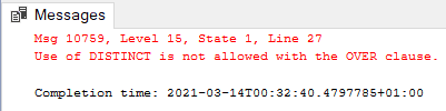
Our problem starts with this query. Count Distinct is not supported by window partitioning, we need to find a different way to achieve the same result.

Planning the Solution

We are counting the rows, so we can use DENSE_RANK to achieve the same result, extracting the last value in the end, we can use a MAX for that. This works in a similar way as the distinct count because all the ties, the records with the same value, receive the same rank value, so the biggest value will be the same as the distinct count.

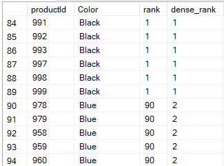
There are two ranking functions: RANK and DENSE_RANK. The difference is how they deal with ties.

RANK: After a tie, the count jumps the number of tied items, leaving a hole.

DENSE_RANK: No jump after a tie, the count continues sequentially

The following query makes an example of the difference:

SELECT productid,
       color,
       Rank()
         OVER (
           ORDER BY color) [rank],
       Dense_rank()
         OVER (
           ORDER BY color) [dense_rank]
FROM   saleslt.product
WHERE  color IS NOT NULL 

The new query using DENSE_RANK will be like this:

SELECT salesorderid,
       Count(*)                          AS ItemsPerOrder,
       Sum(unitprice * orderqty)         AS Total,
       Count(DISTINCT productcategoryid) CategoriesPerOrder,
       Count(DISTINCT color)             ColorPerOrder,
       Dense_rank()
         OVER (
           partition BY productcategoryid
           ORDER BY color )              ColorPerCategory
FROM   saleslt.product p
       INNER JOIN saleslt.salesorderdetail s
               ON p.productid = s.productid
GROUP  BY salesorderid 

However, the result is not what we would expect:

The groupby and the over clause don’t work perfectly together. The fields used on the over clause need to be included in the group by as well, so the query doesn’t work.

Solving the Solution

The first step to solve the problem is to add more fields to the group by. Of course, this will affect the entire result, it will not be what we really expect. The query will be like this:

SELECT salesorderid,
       productcategoryid,
       Count(*)                  AS ItemsPerOrder,
       Sum(unitprice * orderqty) AS Total,
       1                         ColorPerOrder,
       Dense_rank()
         OVER (
           partition BY salesorderid, productcategoryid
           ORDER BY color)       ColorPerCategory
FROM   saleslt.product p
       INNER JOIN saleslt.salesorderdetail s
               ON p.productid = s.productid
GROUP  BY salesorderid,
          productcategoryid,
          color 

There are two interesting changes on the calculation:

  • CategoriesPerOrder was removed, because the group by is some levels below this calculation, we can leave this for later.
  • ColorPerOrder is a fixed value, because we are grouping by colour.

We need to make further calculations over the result of this query, the best solution for this is the use of CTE – Common Table Expressions.

2nd Query Level

The 2nd level of calculations will aggregate the data by ProductCategoryId, removing one of the aggregation levels.

;WITH ranking
     AS (SELECT salesorderid,
                productcategoryid,
                Count(*)                  AS ItemsPerOrder,
                Sum(unitprice * orderqty) AS Total,
                Count(DISTINCT color)     ColorPerOrder,
                Dense_rank()
                  OVER (
                    partition BY salesorderid, productcategoryid
                    ORDER BY color)       ColorPerCategory
         FROM   saleslt.product p
                INNER JOIN saleslt.salesorderdetail s
                        ON p.productid = s.productid
         GROUP  BY salesorderid,
                   productcategoryid,
                   color)
SELECT salesorderid,
       Sum(itemsperorder)    ItemsPerOrder,
       Sum(total)            Total,
       1                     CategoriesPerOrder,
       Sum(colorperorder)    ColorPerOrder,
       Max(colorpercategory) ColorPerCategory
FROM   ranking
GROUP  BY salesorderid,
          productcategoryid 

The calculations on the 2nd query are defined by how the aggregations were made on the first query:

  • ItemsPerOrder: We make a SUM on the results of the COUNT, this will aggregate the different counts.
  • Total: A simple SUM over the SUM already made.
  • CategoriesPerOrder: It can have a fixed number of 1, since we are still aggregating per category
  • ColorPerOrder: We make a SUM over the already existing COUNT from the previous query
  • ColorPerCategory: After making the DENSE_RANK, now we need to extract the MAX value to have the same effect as the COUNT DISTINCT

3rd Query Level

On the 3rd step we reduce the aggregation, achieving our final result, the aggregation by SalesOrderId

;WITH cte
     AS (SELECT salesorderid,
                productcategoryid,
                Count(*)                  AS ItemsPerOrder,
                Sum(unitprice * orderqty) AS Total,
                Count(DISTINCT color)     ColorPerOrder,
                Dense_rank()
                  OVER (
                    partition BY salesorderid, productcategoryid
                    ORDER BY color)       ColorPerCategory
         FROM   saleslt.product p
                INNER JOIN saleslt.salesorderdetail s
                        ON p.productid = s.productid
         GROUP  BY salesorderid,
                   productcategoryid,
                   color),
     cte2
     AS (SELECT salesorderid,
                Sum(itemsperorder)    ItemsPerOrder,
                Sum(total)            Total,
                1                     CategoriesPerOrder,
                Sum(colorperorder)    ColorPerOrder,
                Max(colorpercategory) ColorPerCategory
         FROM   cte
         GROUP  BY salesorderid,
                   productcategoryid)
SELECT salesorderid,
       Sum(itemsperorder)      ItemsPerOrder,
       Sum(total)              Total,
       Sum(categoriesperorder) CategoriesPerOrder,
       Sum(colorperorder)      ColorPerOrder,
       Sum(colorpercategory)   ColorPerCategory
FROM   cte
GROUP  BY salesorderid 

Once again, the calculations are based on the previous queries. Some of them are the same of the 2nd query, aggregating more the rows. However, there are some different calculations:

  • CategoriesPerOrder: It becomes a SUM to achieve the result we would like
  • ColorPerCategory: It becomes a SUM, adding all the distinct count results of each category

The Execution Plan

The execution plan generated by this query is not too bad as we could imagine. This query could benefit from additional indexes and improve the JOIN, but besides that, the plan seems quite ok.

There are other options to achieve the same result, but after trying them the query plan generated was way more complex.

The join is made by the field ProductId, so an index on SalesOrderDetail table by ProductId and covering the additional used fields will help the query

We can create the index with this statement:

CREATE INDEX indorderdetail
  ON saleslt.salesorderdetail (productid)
  include (orderqty, unitprice) 

You may notice on the new query plan the join is converted to a merge join, but the Clustered Index Scan still takes 70% of the query

The secret is that a covering index for the query will be a smaller number of pages than the clustered index, improving even more the query. The statement for the new index will be like this:

CREATE INDEX indproduct
  ON saleslt.product(productid)
  include (productcategoryid, color) 

What’s interesting to notice on this query plan is the SORT, now taking 50% of the query. This doesn’t mean the execution time of the SORT changed, this means the execution time for the entire query reduced and the SORT became a higher percentage of the total execution time.

Further Learning

There will be T-SQL sessions on the Malta Data Saturday Conference, on April 24, register now

Select – Over clause

Common Table Expressions

Describe SQL Server Query Plans

Optimize Query Performance in SQL Server

Conclusion

Mastering modern T-SQL syntaxes, such as CTE’s and Windowing can lead us to interesting magic tricks and improve our productivity


The post Count Distinct and Window Functions appeared first on Simple Talk.


from Simple Talk https://ift.tt/3lhBFFf
via

PowerShell editors and environments part 2

This article is the second of two articles demonstrating PowerShell Editors. The first can be found here. The first article focused on some of the older and more common tools found on both Windows and Linux systems.

This article focuses on more modern tools.

Visual Studio Code

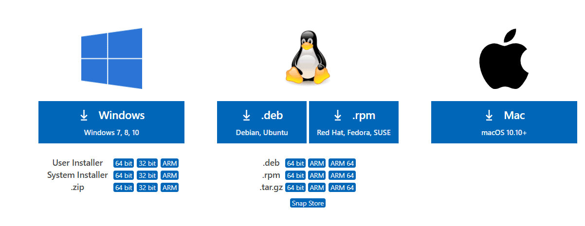
One of the more popular tools these days for creating PowerShell is Visual Studio Code (VS Code). VS Code is not installed by default on most machines but can be downloaded from here: https://code.visualstudio.com/download. One of the first things you will notice is that it is available for multiple platforms as shown in the figure. I will address that in a bit.

Visual Studio Code for Windows

For now, I will assume you are editing PowerShell on Windows 10. If you want to install Visual Studio Code just for yourself, select the 64-bit User Installer; otherwise, select the 64-bit System Installer.

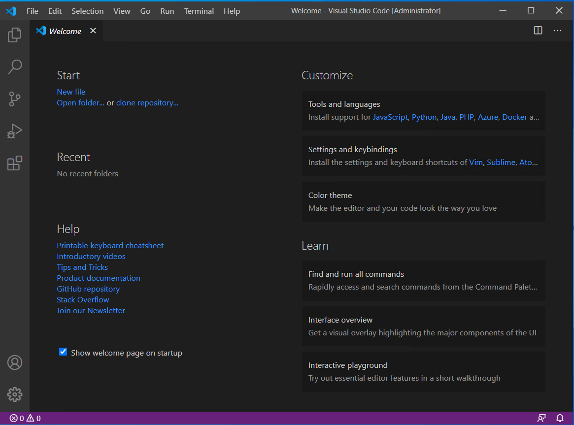
The first time you run Visual Studio Code, you will see something similar to this:

You can create a new file by using the File Menu or pressing Ctrl-N, but there’s another step you should take first.

Click on the button on the left that looks like four boxes with one flying up and to the right: . This icon opens a window that allows you to add extensions to Visual Studio Code. In the Search box that appears, type PowerShell.
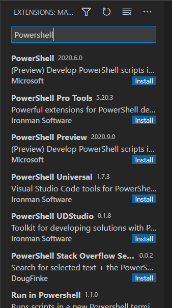

You should see something similar to:

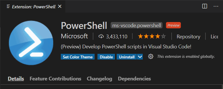
Note that your results may appear different depending on what extensions have been made available since this article was written. Select the topmost one, in this case, PowerShell 2020.6.0, and select Install.

Once installed, you should see something similar in the main area of Visual Studio Code

I’m not a huge fan of the Dark scheme, so I typically select the Set Color Theme and change it to the PowerShell ISE theme. This change makes it look much more like the PowerShell ISE in my previous article.

There is another way to have Visual Studio Code to install the PowerShell extension, and that is simply to open (or create) a file with a .ps1 extension. Visual Studio Code should then provide a pop-up similar to:

As you can see, Visual Studio Code is designed to make it easy for you to get set up to create and edit PowerShell scripts.

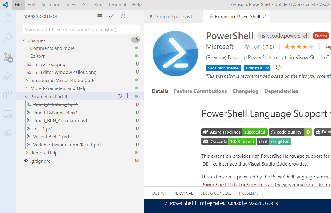
One more step needs to be done to unleash the full power of Visual Studio Code, setting up git.

If you select the Source Control icon you will get a screen like this if you do not have git installed:
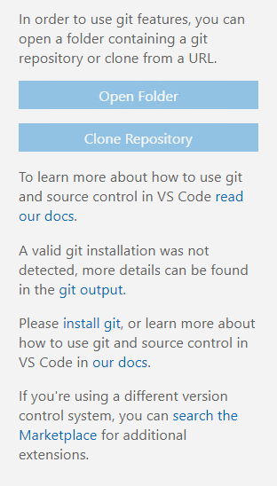
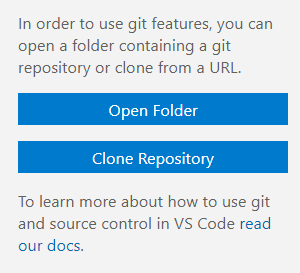
Before you can open a folder or clone a repository, you will need to click on the install git link and follow the prompts. You may need to restart Visual Studio Code after installing and setting up git.

If your screen looks like this:

Git is already configured on your system, and you can open a repository or clone one.

In my case, I have a number of PowerShell Scripts that I have not yet committed to my git repository. Some are scripts I started and abandoned for previous articles, others are ones I’m still working on.

This tight integration with git is the reason the original commenter at the Virtual Pass Summit suggested folks should abandon the PowerShell ISE.

I’m going to be a bit controversial and disagree. Yes, this tight integration is very useful and is a solid argument for using Visual Studio Code. And I do highly encourage you to do so.

That said, how it handles tab completion of parameters is a bit different from the PowerShell ISE. Instead of showing a drop-down of available options in the command-line, you need to press tab to cycle through the parameters and any available validation sets. This isn’t a huge pain, but it does create a bit more work, and I prefer the visual representation the PowerShell ISE provides.

Note it only shows one option at a time. Now the upside: since Visual Studio Code is constantly being updated, perhaps this is a feature that might be updated in the future.

I am not going to go into detail on how to use git in Visual Studio Code in this article. I will add, however, that git is not the only code versioning tool available and that you can most likely find a plug-in for most of the popular tools. Getting on a soapbox for a moment, if you’re not using some form of version control, even for simple PowerShell scripts, you should definitely start doing so.

Visual Studio Code for Linux

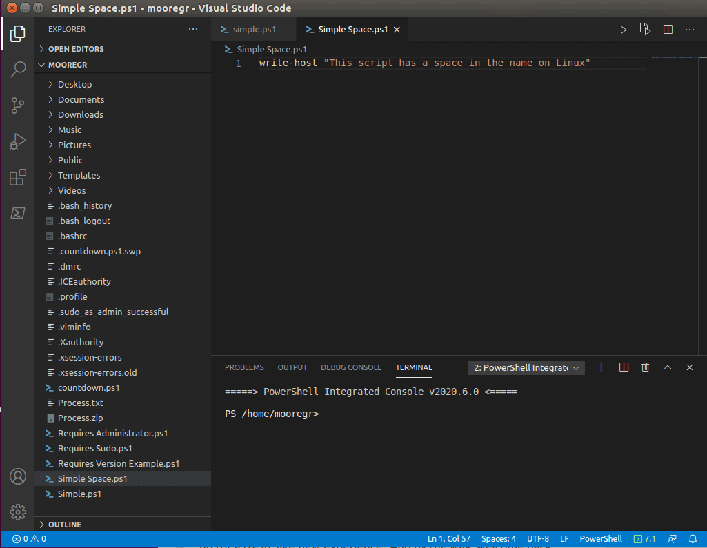
Again, because Microsoft has committed to being cross-platform, it is entirely possible to install Visual Studio Code on Linux. The installation steps vary based on the distribution of Linux you are running. In my case, I am running Ubuntu, so I chose the GUI installed option at the URL: https://code.visualstudio.com/docs/setup/linux

As you can see, this looks almost exactly like the Dark Mode theme for Visual Studio on Windows. From a functionality point of view, Visual Studio Code is basically the same. There may be some differences in how case-sensitivity is handled, but you will find moving from one platform to another is a trivial exercise.

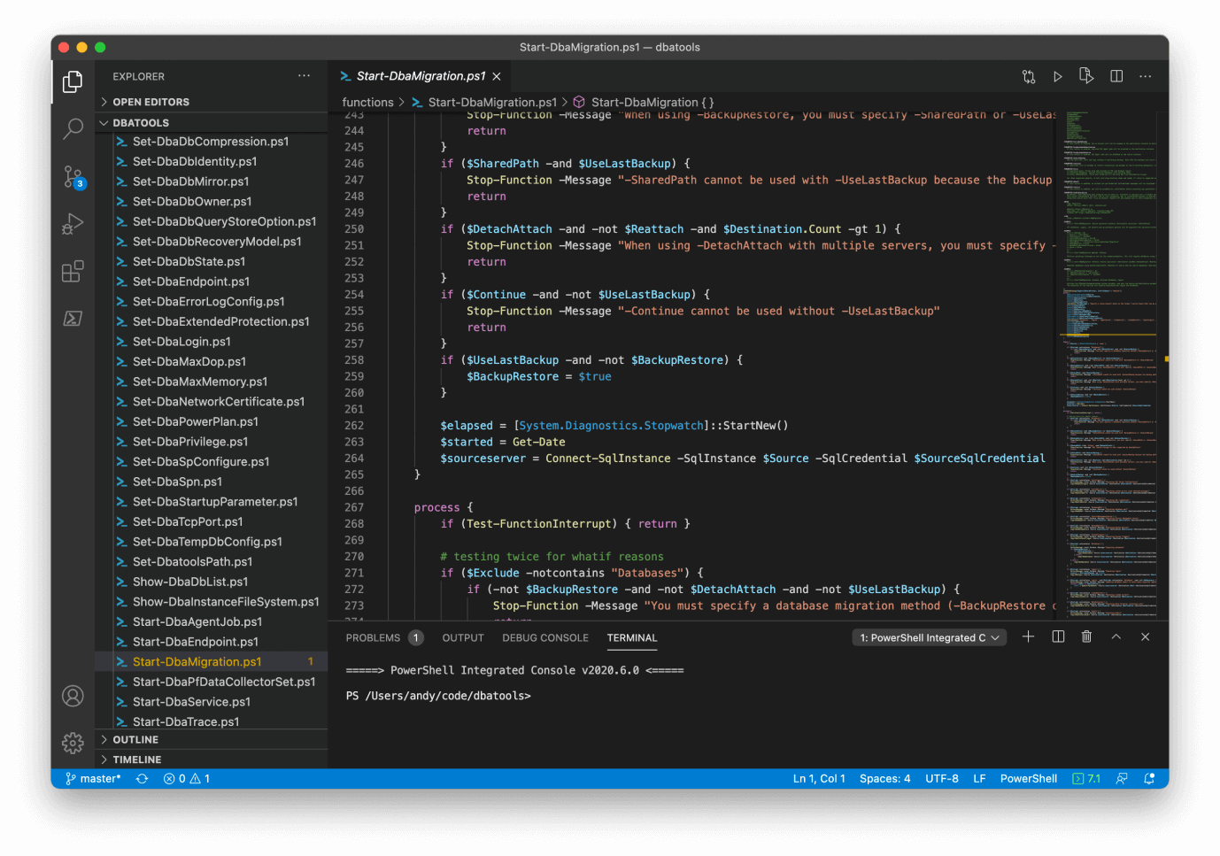
Visual Studio Code for the Mac

I don’t have a running Mac environment, so I had to rely on a screenshot from fellow DBA Andy Levy:

https://apps.rackspace.com/api/mail/v1/users/mooregr@greenms.com/messages/SU5CT1g=.332556/attachments/2.2?csrf=c47b9c912b4d4a9cafe0421560b3cd8d&wsid=4abfa09978d64a7fb167eb60dee5f408-8dc41fb5ec7b40bcb6863fad1d7e6378

With minor exceptions, as you can see, it’s again the same basic interface as on Windows and Linux.

Microsoft has committed to making Visual Studio Code a cross-platform tool that can be used without retraining developers for each platform.

Visual Studio Code for the Android

Ok, this one doesn’t seem to exist. Yet. But I wouldn’t be surprised if it’s available someday.

Some Features of Visual Studio Code

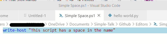
As powerful as VS Code is, it does not automatically know what language you’re typing something in unless you tell it. The most common way is to create a file with the extension of the file language you want to run.

In the above example, I have both a PowerShell file and a Python file open. When I hit F5 or the Execute icon, VS Code should automatically determine which interpreter run and run the script. If for some reason it asks you, you may need to set the terminal type in the lower half of the screen:

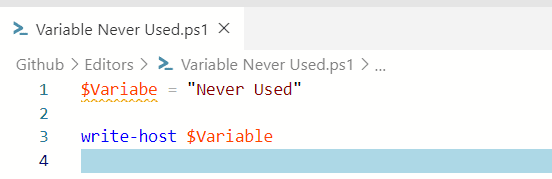
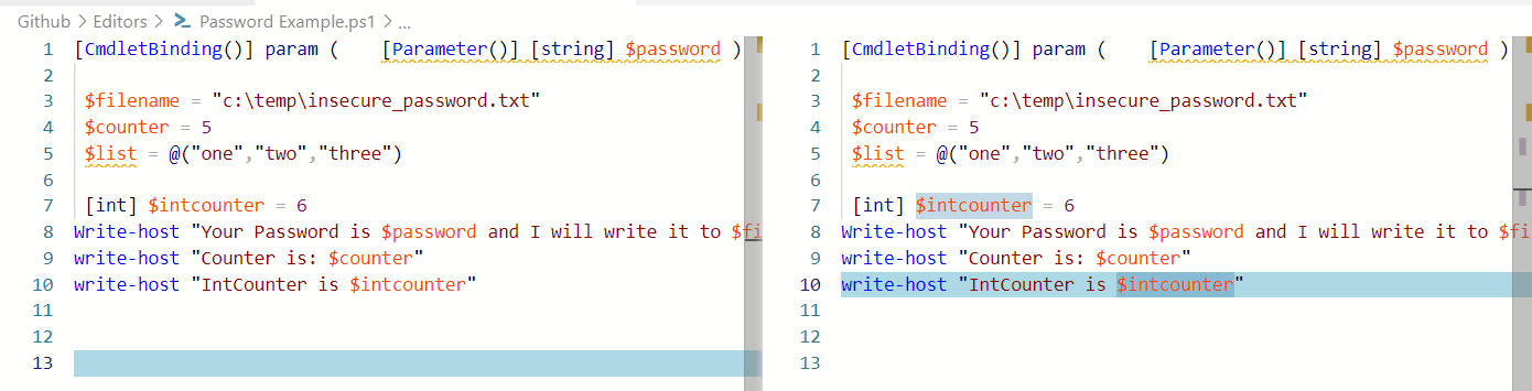
Since Visual Studio Code is intended as an actual IDE, unlike PowerShell ISE, it has many useful features. For example, it will highlight variables that are unused or may have other issues.

Here you can see that it warns that the variable is never used. This warning may indicate the code has changed and that variable is no longer needed or that the variable has a typo in it. In the above example, I left out the L. This is a trivial example, but if the script were dozens of lines long, you might not notice the difference unless you were warned.

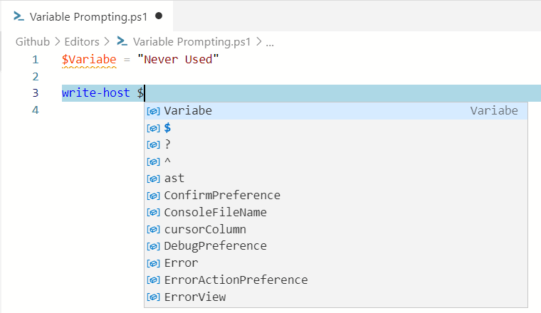
However, VSC is even more helpful in making sure you avoid such mistakes.

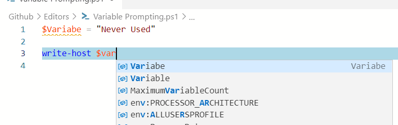
As you start to type a variable name, it will helpfully prompt you for possible variables. Here you can see it’s showing a list of variables you might want to use. Tab completion will select the highlighted one. As you type more characters, VSC will refine its options

Note that it shows Variable as an option because I had previously defined that in an earlier script, and it is persisting in memory.

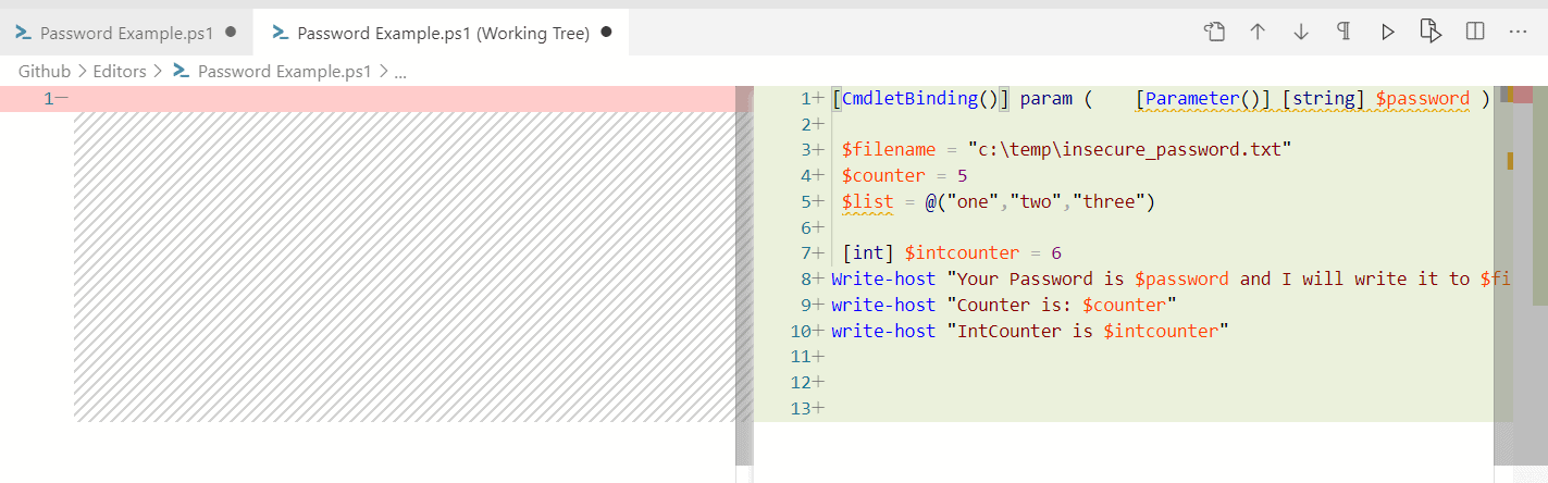
Another example of it trying to help protect you is if you want to pass a password into a script, it will guard against using a non-secure string:

There are a couple of other features I want to point out in VS Code. After clicking the Files icon, you will see an option at the bottom of the Explorer window (you may need to expand it by hitting the > symbol) for a Timeline. In the previous example, I have not yet committed this script to git, so I see:

If I click on Uncommited Changes, I will see a history of my changes:

Since I have git set up, I can go to the version control icon and find the file in question:
And either revert the changes or commit them. In this case, I want to stage them using the + (plus) symbol. I then need to commit them using the option at the top. Remember, you always need to have a message with your commits. And if you’re using a remote repository, you need to push to it. Again, all the details of how to use git are beyond the scope of this article.

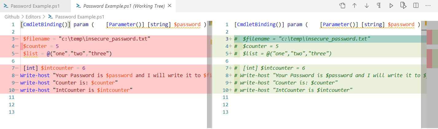
Once I commit my change, however, my history window now shows both sides as the same.

If I decide to make changes, now I can see what changes I’ve made by again going to my version control tab and selecting the file in question to see the changes.

Visual Studio Code is a full-fledged modern IDE with all the bells and whistles, not only for PowerShell but also for many other languages. If you’re not using it or something similar for your PowerShell development, you really should!

Azure Data Studio

Azure Data Studio has become increasingly popular. Despite the name, you don’t need to actually have an Azure account to use it.

You can download and install the latest version from here. Again, something you will notice is that it’s available across all three major OSes.

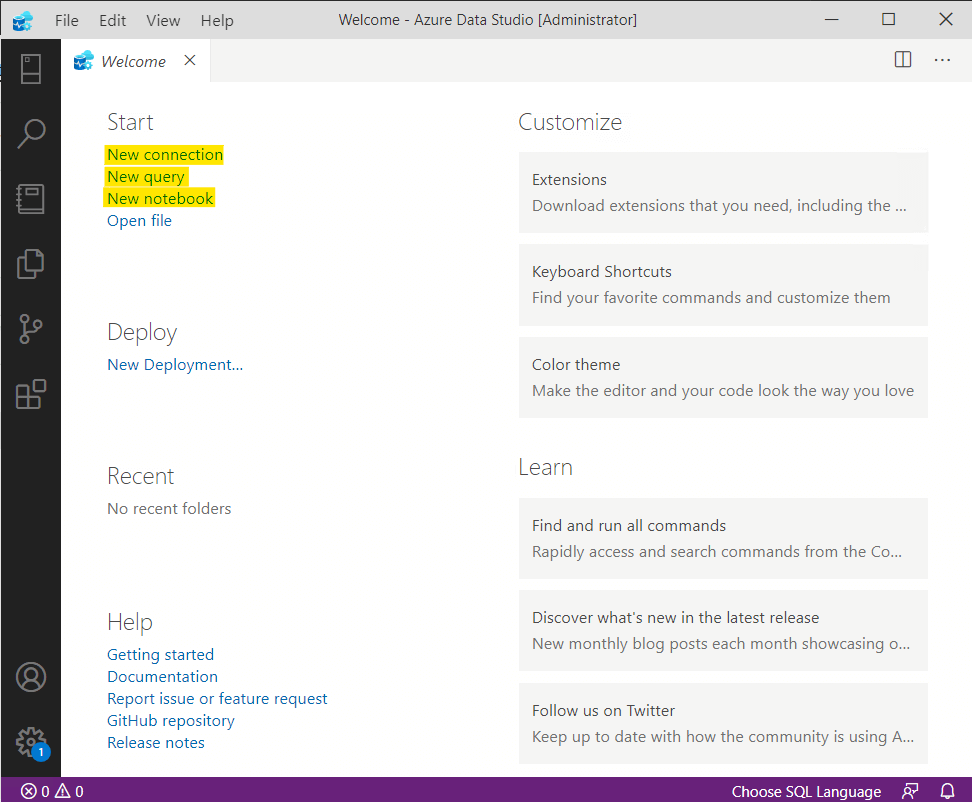
When you first open it, you’ll see it looks very similar to Visual Studio Code because it is built on it. However, there are some differences. The ones that are important for this article are highlighted below.

Since Azure Data Studio is built on VS Code, you can install and run the PowerShell Kernel just as you did above. But that’s not where you will see one of the biggest advantages of Azure Data Studios. This advantage is the ability to create Notebooks as demonstrated below.

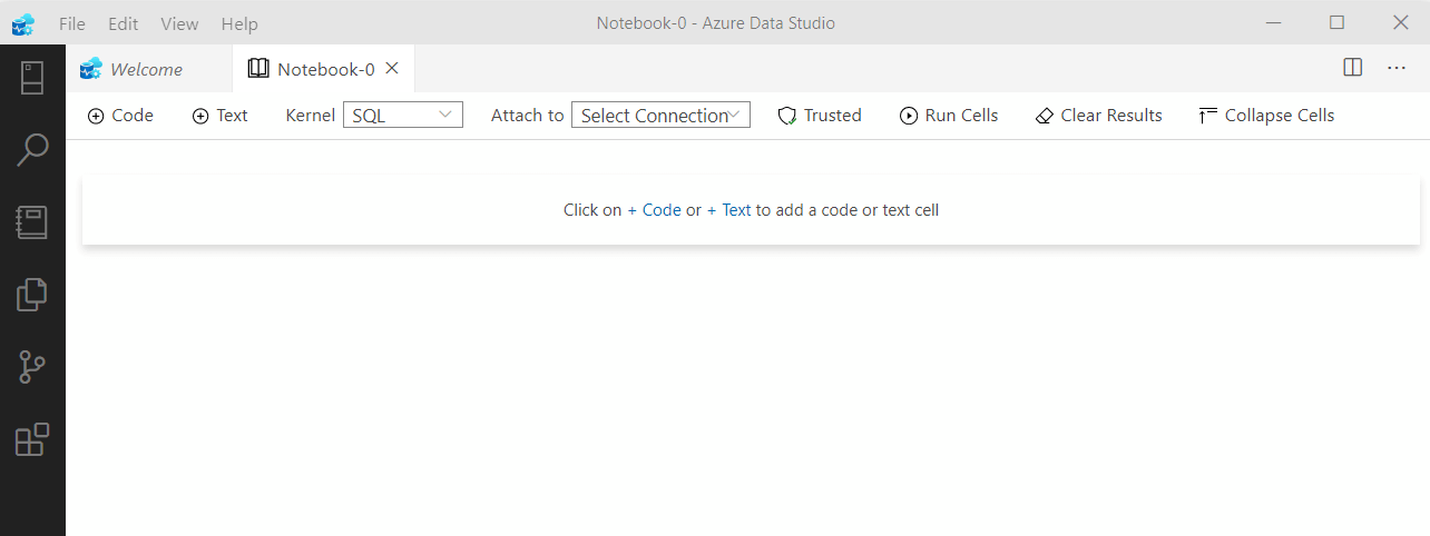
For now, simply select New Notebook.

Again, this should look familiar. In this case, you will need to select a new kernel: PowerShell.

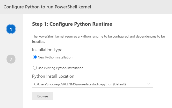
Python is required for the PowerShell functionality. If you have not previously installed Python, you will be prompted to do so. You will get a prompt similar to the following:

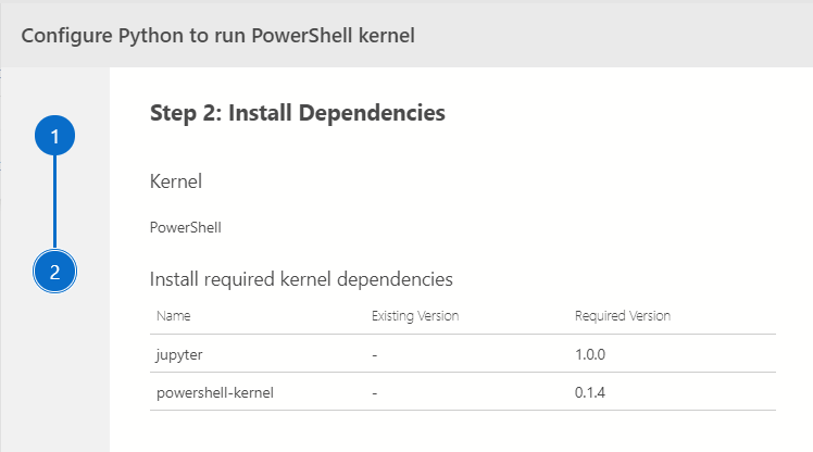
If you have dependencies, go ahead and install them.

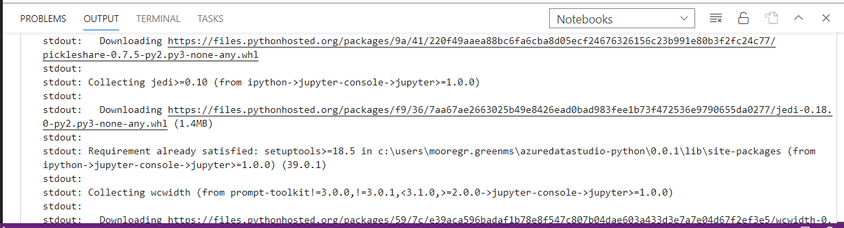
The installs will take several minutes, and you’ll see a number of messages in your output window as it installs.

Example output.

At this point, if you’re familiar with Jupyter Notebooks, all of this, especially the Python install, should look familiar. If you’re not familiar with Jupyter Notebooks, that’s fine, but understand that Azure Data Studio with PowerShell is basically built on top of the Jupyter Framework but gives you even more power.

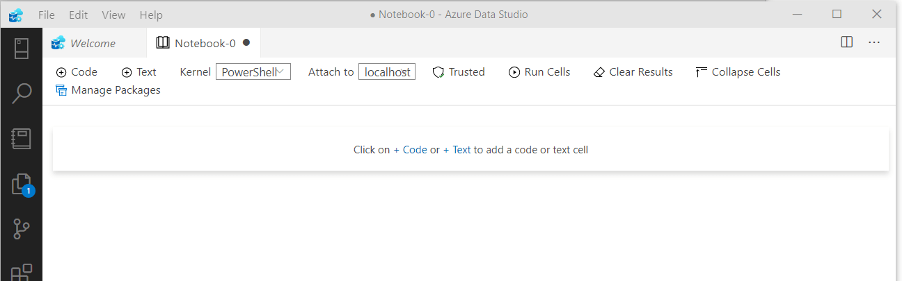
Once everything is installed, however, you should see that your selected kernel is now PowerShell.

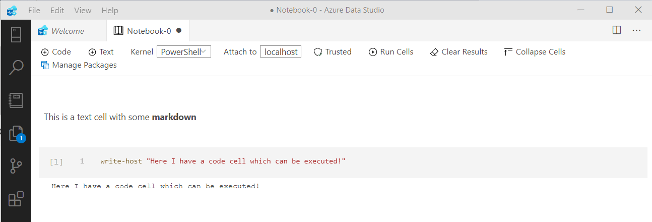
The notebook will prompt you to create a Code or Text cell. A text cell is just as you would expect, an area where you can enter text. You can use markdown or the built-in formatting tools to format the text in various ways. A text cell does not run code.

However, a Code Cell is an area where you can enter code in the language of your choice (in this case, PowerShell) and then execute it.

This example is rather trivial, and you may wonder what’s the advantage or use of Azure Data Studio.

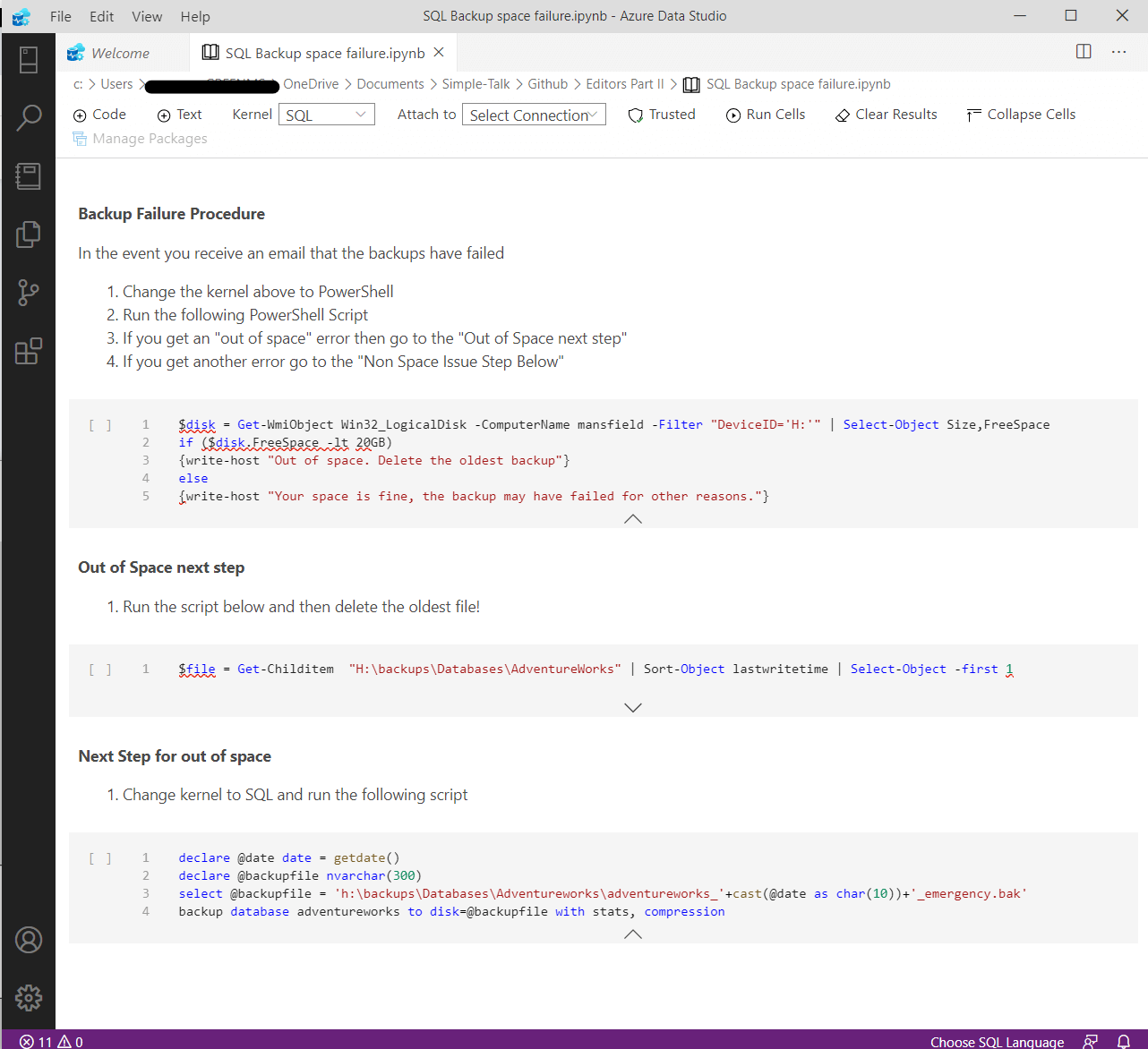
In a previous life, I was Director and then later a VP of IT at two different Internet startups. I managed teams of people who, among other things, had the duty of keeping our servers online 24/7. This commitment meant responding to problems and developing playbooks to share knowledge among team members. I wish I had something like Jupyter Notebooks or Azure Data Studio back then because if I did, creating something like the following would have been both very handy and fairly trivial to create.

Not only do I have a playbook that documents the procedure, but also allows the person to execute the necessary steps from within the playbook! This is very useful!

Some of my fellow presenters are starting to use this for their presentations also, so they can have their talking points and demonstrations in a single place.

At the start of the section, I mentioned you do not need an Azure account, but if you do, you can write playbooks that can run both PowerShell and T-SQL scripts against your Azure instances. However, it is important to understand that while each individual code cell can run a different language you do need to switch between kernels if the language of the cell is different. In the above example, the first two code cells are PowerShell Scripts and the final one is a T-SQL script. As you can imagine, this can be a very powerful ability to have.

PowerShell Editors and Environments

When I set out to write an article on PowerShell editors and environments, I originally planned a single article. It quickly became apparent, however, that there was enough for two full articles complete with examples. Even then, I’ve found I’ve only touched upon the surface of what can be done. I think this illustrates in part how important PowerShell has become and how it absolutely should be treated as importantly as T-SQL is to a DBA, or C# is to a developer. It’s a real, full-fledged language. When I first started using PowerShell nearly a decade ago, I started with Notepad and tried to execute scripts at the PS command line, Scripts for the most part, tended to be quick one-offs of maybe 5-10 lines. Now scripts are often full-fledged programs, complete with GUI support (at least on Windows) under version control (using git or similar tools) developed in full-fledged editors.

Hopefully, these two articles have exposed you to more options, and you can choose the proper tool to solve your problem.


The post PowerShell editors and environments part 2 appeared first on Simple Talk.


from Simple Talk https://ift.tt/30Hxw3Y
via

The Issue\Purpose of Multiple Edge Constraint/Conditions

Edge constraints were added in SQL Server 2019 to make the node to edge relationship stricter/enforced, and more like typical foreign key constraints. When used, they define what node types can be used in the from and to position of the edge. What makes edges different than a many-to-many relationship in a relational table is that an edge can implement more than one many-to-many relationship in a single table. To constrain the types of data that can be put into the edge, you can use an edge constraint.

Edge constraints are very similar to implementing foreign key constraints, but there are a few key differences. Foreign keys are between two tables. Edges are between one edge table, and multiple pairs of node tables. In both cases, you can have multiple constraints, even from the same table to the same related table on the same column. However, with edge constraints, because you can have multiple pairs of expressions, and even multiple constraints, it bears discussion. If you have more than one constraint, it has one big negative, but it is allowed to implement one big positive!

Take for example, the following two nodes:

CREATE TABLE dbo.Node1(Name varchar(20)) AS NODE;
CREATE TABLE dbo.Node2(Name varchar(20)) AS NODE;

INSERT INTO  dbo.Node1(Name)  VALUES ('One'),('Two');
INSERT INTO  dbo.Node2(Name)  VALUES ('Buckle'),('Shoe');

When I built my first edge with an edge constraint, I thought, what if I want the constraint do cascading deletes for one relationship but prevent deletes in others. So, I built this:

CREATE TABLE dbo.Edge1
(
        CONSTRAINT EC_Edge1_1 CONNECTION (dbo.Node1 TO dbo.Node1,
                                          dbo.Node2 TO dbo.Node2) 
                             ON DELETE NO ACTION,
        CONSTRAINT EC_Edge1_2 CONNECTION (dbo.Node2 TO dbo.Node1) 
                             ON DELETE CASCADE
) AS EDGE;

Much like you would do with a foreign key constraint. But when you try to insert any data…

--from node1 to node1 fails:
INSERT INTO dbo.Edge1($from_id, $to_id)
SELECT (SELECT $node_id FROM dbo.Node1 WHERE name = 'One'),
       (SELECT $node_id FROM dbo.Node1 WHERE name = 'Two');

Results in this:

Msg 547, Level 16, State 0, Line 30
The INSERT statement conflicted with the EDGE constraint "EC_Edge1_2". 
The conflict occurred in database "tempdb", table "dbo.Edge1".

And this:

INSERT INTO dbo.Edge1($from_id, $to_id)
SELECT (SELECT $node_id FROM dbo.Node2 WHERE name = 'Buckle'),
       (SELECT $node_id FROM dbo.Node1 WHERE name = 'One');

Violates the other constraint:

Msg 547, Level 16, State 0, Line 40
The INSERT statement conflicted with the EDGE constraint "EC_Edge1_1". 
The conflict occurred in database "tempdb", table "dbo.Edge1".

Microsoft docs states:

  • If multiple edge constraints are created on a single edge table, edges must satisfy ALL constraints to be allowed.

So you cannot actually do this and get an additive configuration like a foreign key constraint. Rather, the value of allowing multiple constraints is designed to be when adding a new condition. Say your edge was:

DROP TABLE dbo.Edge1;
CREATE TABLE dbo.Edge1
(
        CONSTRAINT EC_Edge1 CONNECTION (dbo.Node1 TO dbo.Node1)                           
                                  ON DELETE NO ACTION,
) AS EDGE;

Now you can insert:

INSERT INTO dbo.Edge1($from_id, $to_id)
SELECT (SELECT $node_id FROM dbo.Node1 WHERE name = 'One'),
       (SELECT $node_id FROM dbo.Node1 WHERE name = 'Two');

But still not:

INSERT INTO dbo.Edge1($from_id, $to_id)
SELECT (SELECT $node_id FROM dbo.Node2 WHERE name = 'Buckle'),
       (SELECT $node_id FROM dbo.Node1 WHERE name = 'One');

Which causes this error that still conflicts with the EC_Edge1 constraint:

Msg 547, Level 16, State 0, Line 70
The INSERT statement conflicted with the EDGE constraint "EC_Edge1". 
The conflict occurred in database "tempdb", table "dbo.Edge1".

However, to add in the new, Node2 to Node1 rows, you execute:

ALTER TABLE dbo.Edge1
  ADD CONSTRAINT EC_Edge1_NEW CONNECTION 
                                  (dbo.Node1 TO dbo.Node1,
                                   dbo.Node2 TO dbo.Node1) 
                            ON DELETE NO ACTION;

This still won’t work:

INSERT INTO dbo.Edge1($from_id, $to_id)
SELECT (SELECT $node_id FROM dbo.Node2 WHERE name = 'Buckle'),
       (SELECT $node_id FROM dbo.Node1 WHERE name = 'One');

Until you drop the original edge constraint:

ALTER TABLE dbo.Edge1 DROP CONSTRAINT EC_Edge1;

And the INSERT will now work. You can rename the constraint and all is well:

EXEC sp_rename 'EC_Edge1_NEW','EC_Edge1';

At first glance this feels very silly. Why not drop the constraint and add the new one? The value lies in the fact that when you added EC_Edge1_NEW with a new condition, because there already was an existing, trusted constraint, the Node1 to Node1 condition need not be rechecked, potentially saving quite a bit of processing time when adding a new constraint.  This is the big positive, and as long as you understand that 2 constraints are not additive, is a great thing for your administrative tasks on larger objects.

The post The Issue\Purpose of Multiple Edge Constraint/Conditions appeared first on Simple Talk.


from Simple Talk https://ift.tt/3cAAPQ5
via