Tuesday, November 16, 2021

BETWEEN the two of us

This past August, I was looking at an online SQL tutorial. One of the sessions in it featured the

BETWEEN predicate, which brought back some memories. In the early days of SQL on the ANSI X3H2 Database Standards Committee, we created the BETWEEN predicate. We wanted the SQL language to sound a bit like English and have shorthand terms for common coding situations. Many of our keywords were stolen from other programming languages or deliberately chosen so that they were not likely to be confused with data elements. The original syntax for the between predicate looks like this:

BETWEEN::=
<test_expression> [NOT] BETWEEN
 <begin_expression> AND <end_expression>

The BETWEEN predicate specifies the inclusive range to test the expression values. The range is defined by boundary expressions with the AND keyword BETWEEN them. Naturally, all the expressions in BETWEEN predicate must be the same data type or cast to it, as in the case of any comparison predicate. This predicate Is defined as a shorthand for:

(<test_expression> >= <begin_expression> 
AND <test_expression> <= <end_expression>)

And the negated version of the predicate

<test_expression> NOT BETWEEN <begin_expression> AND <end_expression>

is equal to:

NOT (<test_expression> BETWEEN <begin_expression> AND <end_expression>)

The grammar for SQL is deliberately picked to be LALR(1). If you don’t remember that from your compiler writing classes, don’t feel bad. It means that SQL can have a little more complicated grammar than many programming languages to sprinkle keywords In places a little more like natural English. It’s important to notice that the BETWEEN predicate uses a closed interval, which includes the endpoints of the range. However, the NOT BETWEEN excludes them.

<test_expression> NOT BETWEEN <begin_expression> AND <end_expression>

is equivalent to

(<test_expression> < <begin_expression> 
OR <test_expression> > <end_expression>)

At some point in these early days, one of the committee members proposed changing the syntax and creating what would now be called a “symmetric BETWEEN” as the default definition. This proposal passed because committees love proposals. Only Microsoft implemented this feature in their Access tabletop database. All the other vendors ignored it, and the proposal was rescinded at the next committee meeting.

But proposals with extended features seem to keep coming back to life. The current ANSI/ISO standard syntax is:

<test_expression> [NOT] BETWEEN [SYMMETRIC | ASYMMETRIC] 
<begin_expression> AND <end_expression>

The keyword ASYMMETRIC has the original functionality, and it is optional. The BETWEEN SYMMETRIC syntax is like BETWEEN except that there is no requirement that the argument to the left of the AND be less than or equal to the argument on the right. Well, not entirely: officially, the <begin_expression> is the minimum, and the <end_expression> is the maximum. This transformation converts a SYMMETRIC BETWEEN into a regular old vanilla BETWEEN.

Intervals in the ISO data model

Several ISO standards deal with the concepts of intervals. From a mathematical viewpoint, the kinds of intervals you can have are (1) Closed, (2) Opened, (3) Half open high, and (4) Half open low. A closed interval includes both the endpoints, like the range in the BETWEEN predicate. An open interval excludes both the endpoints of the range, like the NOT BETWEEN predicate. The half open intervals are open on either the high-end or the low end of the interval range.

A half open interval on the high-end is how ISO models time. We talk about “24-hour time” Or “military time,” but the truth is a day is defined as an interval from 00:00:00 up to 23:59:59.999.. at whatever precision can be measured. If you try and put in “24:00:00 Hrs”, DB2 and other databases will automatically convert it to 00:00:00 Hrs of the next day. Think of it as being like converting a person’s height from 5’18” to 6’6” instead. These conventions get even stranger when you look at how different countries and cultures handle times greater than one day. If an event in Japan runs past midnight, they simply add more hours to the event. For example, an event that ran past midnight might be shown as “25:15:00 Hrs.”

The advantage of the half open interval is easy to see in the ISO 8601 standards, which define how temporal data is represented. You are always sure when an event starts, even if you’re not sure when it will end, so you can use a NULL to mark the end of an event that is in process. This NULL can be coalesced to a meaningful value. For example, sometimes it might make sense to use COALESCE(interval_final_timestamp, CURRENT_TIMESTAMP) To figure out the duration of the interval at exactly the moment the query is invoked. Other times, you might want to use COALESCE(interval_final_timestamp, legally_defined_stop_timestamp).

The BETWEEN predicate is not just used for timestamps. It works perfectly well for numeric ranges and text, too. Numeric ranges can be used to throw things into buckets, which looks reasonably obvious until the three parameter values are of different numeric types. Now you have to consider rounding and casting errors. Even worse, if the parameters are character data with different correlations. As a generalization, you really need to make sure that all three parameters are of the same type. In fact, ranges and text data can get so complicated, I’m just going to ignore them. Let’s just look at numeric ranges.

Report cards

A classic example of reducing values into ranges is converting grades from numeric totals or percentages to a letter grade. The usual convention is that a score in the 90s is an “A”, a score in the 80s is a “B”, a score in the 70s is a “C”, a score in the 60s is a “D” and anything below that is an “F”. I’m choosing to ignore plus or minus options on the letters.

The CASE expression in SQL is executed from left to right, and the first WHEN clause that tests TRUE returns the value in its THEN clause. This means that the order in which you write your tests will control how it executes; not all programming languages work this way. In effect, we have hard-coded half open intervals.

CASE
WHEN score >= 90.000 THEN ‘A’
WHEN score >= 80.000 THEN ‘B’
WHEN score >= 70.000 THEN ‘C’
WHEN score >= 60.000 THEN ‘D’
ELSE ‘F’ END

It is important to notice that this expression will handle somebody who has more than 100 points to qualify as an “A” student. In this example, that’s probably what was intended for extra credit, but this might indicate an error in the data in other schemes. Likewise, a score of zero might be a data error. Then, of course, because this is SQL, what would a NULL mean? Perhaps it indicates an incomplete? A general rule of thumb is to design for the extreme cases but tuning for the most expected cases.

The OVERLAPS() predicate

The OVERLAPS predicate is part of the SQL Standards but not part of SQL Server. This predicate is defined only for temporal data and is based on temporal intervals. Yes, there is a temporal interval type in Standard SQL. Before getting into it, we need to back up and discuss something known as Allen’s operators. They are named after J. F. Allen, who defined them in a 1983 research paper on temporal intervals. The basic model has two temporal intervals, expressed as ordered pairs of start and termination timestamps (S1, T1) and (S2, T2).

Here are the base relations between two intervals, as timelines.
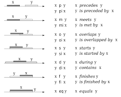
An images showing base relations between two intervals, as timelines.

SQL did not add all 13 relationships, but we decided that an overlaps predicate would be the most useful.

The result of the <OVERLAPS predicate> is formally defined as the result of the following expression:

(S1 > S2 AND NOT (S1 >= T2 AND T1 >= T2))
 OR (S2 > S1 AND NOT (S2 >= T1 AND T2 >= T1))
 OR (S1 = S2 AND (T1 <> T2 OR T1 = T2))

where S1 and S2 are the starting times of the two time periods and T1 and T2 are their termination times. The rules for the OVERLAPS() predicate sound like they should be intuitive, but they are not. The principles that we wanted in the Standard were:

1. A time period includes its starting point but does not include its end point. We have already discussed this model and its closure properties.

2. If the time periods are not “instantaneous,” they overlap when they share a common time period.

3. If the first term of the predicate is an INTERVAL, and the second term is an instantaneous event (a <datetime> data type), they overlap when the second term is in the time period (but is not the end point of the time period). That follows the half-open model.

4. If the first and second terms are instantaneous events, they overlap only when they are equal.

5. If the starting time is NULL and the finishing time is a <datetime> value, the finishing time becomes the starting time, and we have an event. If the starting time is NULL and the finishing time is an INTERVAL value, then both the finishing and starting times are NULL.

Please consider how your intuition reacts to these results when the granularity is at the YEAR-MONTH-DAY level. Remember that the day begins at 00:00:00 Hrs.

(today, today) OVERLAPS (today, today) = TRUE
 (today, tomorrow) OVERLAPS (today, today) = TRUE
 (today, tomorrow) OVERLAPS (tomorrow, tomorrow) = FALSE
 (yesterday, today) OVERLAPS (today, tomorrow) = FALSE

Contiguous temporal intervals with DDL

Alexander Kuznetsov wrote this idiom for History Tables in T-SQL, but it generalizes to any SQL. It builds a temporal chain from the current row to the previous row with a self-reference. This is easier to show with code:

CREATE TABLE Tasks
(task_id INTEGER NOT NULL,  --  makes sense in your data
 task_score CHAR(1) NOT NULL,  -- whatever makes sense in your data
 previous_end_date DATE, -- null means first task
 current_start_date DATE DEFAULT CURRENT_TIMESTAMP NOT NULL,
 CONSTRAINT previous_end_date_and_current_start_in_sequence
   CHECK (prev_end_date <= current_start_date)
 DEFERRABLE INITIALLY IMMEDIATE,
 current_end_date DATE, -- null means unfinished current task
 CONSTRAINT current_start_and_end_dates_in_sequence
   CHECK (current_start_date <= current_end_date),
 CONSTRAINT end_dates_in_sequence
   CHECK (previous_end_date <> current_end_date),
 PRIMARY KEY (task_id, current_start_date),
 UNIQUE (task_id, previous_end_date), -- null first task
 UNIQUE (task_id, current_end_date), -- one null current task
 FOREIGN KEY (task_id, previous_end_date)  -- self-reference
   REFERENCES Tasks (task_id, current_end_date));

Well, that looks complicated! Let’s look at it column by column. Task_id explains itself. The previous_end_date will not have a value for the first task in the chain, so it is NULL-able. The current_start_date and current_end_date are the same data elements, temporal sequence, and PRIMARY KEY constraints we had in the simple history table schema.

The two UNIQUE constraints will allow one NULL in their pairs of columns and prevent duplicates. Remember that UNIQUE is NULL-able, not like PRIMARY KEY, which implies UNIQUE NOT NULL.

Finally, the FOREIGN KEY is the real trick. Obviously, the previous task has to end when the current task started for them to abut, so there is another constraint. This constraint is a self-reference that makes sure this is true. Modifying data in this type of table is easy but requires some thought.

There is just one little problem with that FOREIGN KEY constraint. It will not let you put the first task into the table. There is nothing for the constraint to reference. In Standard SQL, we can declare constraints to be DEFERABLE with some other options. The idea is that you can turn a constraint ON or OFF during a session so the database can be in a state that would otherwise be illegal. But at the end of the session, all constraints have to be TRUE or UNKNOWN.

When a disabled constraint is re-enabled, the database does not check to ensure any existing data meets the constraints. You will want to hide this in a procedure body to get things started.

BETWEEN

Please notice that the OVERLAPS and BETWEEN predicates work with static intervals, but there are also dynamic predicates for data. The LEAD and LAG operators view the rows as representing points in time or in a sequence, but that is a topic for another article.

If you liked this article, you might also like A UNIQUE experience


The post BETWEEN the two of us appeared first on Simple Talk.


from Simple Talk https://ift.tt/3Dwab6Q
via

Using SQL Server sequence objects

A SQL Server sequence object is an object that can be used to produce a series of integer values based on a starting point and an increment value. They are similar to identity columns but are more flexible. It’s possible to use multiple sequences to populate more than one column in a table. One sequence object can also be used across multiple tables in a database. This article walks you through using SQL Server sequence objects.

The sequence object was introduced to SQL Server with the rollout of SQL Server 2012. In part 1 of the sequence object series, I discussed the basics of using the sequence object. This article covers the more advanced topics like how to control caching and cycling sequence numbers and more.

Using default values

When creating a sequence object, only the sequence name argument is required. For any parameter not specified, the default value for that option will be used. I will discuss a few of those default values that might surprise you.

The default data type for a sequence object is bigint. Using a sequence object to populate a smaller integer column data type might cause an error. The error occurs when the sequence number generated is larger or smaller thn supported by the target column data type.

The MINVALUE and MAXVALUE default values are set based on the sequence object’s data type. For instance when a sequence object is defined as a bigint the MINVALUE is set to -9,223,372,036,854,775,808 and the MAXVALUE is set to 9,223,372,036,854,775,807.

The last one worth mentioning, is the START WITH parameter. This parameter identifies the first sequence number that will be generate. The default value for starting value is determined by the wheter the INCREMENT value is positive or negative. If the INCREMENT BY parameter is negative, then the START WITH value is set to maximum value of data type for the sequence object. For a sequence objects that count up, the default starting value is set to the minimum value for the object’s data type.

For a complete list of all sequence object parameter defaults refer to the Microsoft Documentation.

Using a sequence object to support multiple tables

One of the advantages of using sequence objects is that one sequence object can be used in multiple tables. Suppose you have a business requirement to track issues, where each issue requires a unique issue number. Additionally, the issue number needs to be stored in different tables based on the type of issue.

To test out these requirements, assume there are two different types of issues to track: hardware and service. The hardware issues are stored in the HardwareIssue table, and service issues are stored in the ServiceIssue table. The code in Listing 1 is used to create the IssueNumber sequence object and the HardwareIssue and ServiceIssue tables.

Listing 1: Creating Hardware and Service table

USE tempdb;
GO
-- Create Sequence Object
CREATE SEQUENCE IssueNumber
      START WITH 1
      INCREMENT BY 1; 
GO
-- Create tables to track issues
CREATE TABLE HardwareIssue (
IssueNumber INT NOT NULL 
      CONSTRAINT [DF_HardwareIssueNumber] DEFAULT 
        (NEXT VALUE FOR IssueNumber),
IssueDescription VARCHAR (1000), 
IssueDate DATETIME);
CREATE TABLE ServiceIssue (
IssueNumber INT NOT NULL 
      CONSTRAINT [DF_ServiceIssueNumber] DEFAULT 
         (NEXT VALUE FOR IssueNumber),
IssueDescription VARCHAR (1000), 
issueDate DATETIME);
GO

A default constraint was also defined with each IssueNumber column, which references the IssueNumber sequence object. The IssueNumber column will be automatically populated when a new row is added by having a default value.

Run the code in Listing 2 to test that each of these tables will automatically populate the IssueNumber columns using the IssueNumber sequence object.

Listing 2: Inserting a Few Rows into both test tables

INSERT INTO HardwareIssue (IssueDescription, IssueDate)
   VALUES ('Bad power supply', getdate());
INSERT INTO ServiceIssue (IssueDescription, IssueDate)
   VALUES ('Unable to contact vendor for service',getdate());
INSERT INTO HardwareIssue (IssueDescription, IssueDate)
   VALUES ('Disk drive getting errors',getdate());
INSERT INTO ServiceIssue (IssueDescription, IssueDate)
   VALUES ('Looking for help with Server',getdate());
SELECT * FROM HardwareIssue;
SELECT * FROM ServiceIssue;

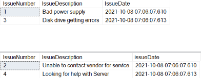
Output from running Listing 2 can be found in Report 1.

Report 1: Output from running Listing 2.

Image showing the results of inserting into the two tables with one sequence object

This example showed one way a sequence object can be used to populate columns in multiple tables. But it also showed how by using a default constraint, you can automatically generate the IssueNumber value without providing that value on an INSERT statement.In Report 1, the first set of records displayed are from the HardwareIssue table, and the second set of records are from the ServiceIssue table. By looking at the IssueNumber column in the output, you can see that each value is unique across both tables.

Recycling sequence numbers

Sequence numbers can be recycled by setting the CYCLE option. When the CYCLE option is turned on the sequence number will restart once the maximum or minimum values is reached, depending on whether the increment value is a positive or negative integer value.

To demonstrate recycling a sequence number, I’ll create a new sequence object using the code in Listing 3.

Listing 3: Creating sequence object

USE tempdb;
GO
CREATE SEQUENCE RecycleEvery2
      START WITH 1
      INCREMENT BY 1
          MINVALUE 1
          MAXVALUE 2
          CYCLE; 
GO

In Listing 3, the sequence object created is named RecycleEvery2. This sequence object will start at 1 and will recycle the value when it reaches 2. The keyword CYCLE in the CREATE SEQUENCE statement tells SQL Server that this sequence object needs to be recycled after it reaches the maximum value.

When the CYCLE option is not specified at creation, as in Listing 1, the sequence number defaults to NO CYCLE. If a sequence object is defined to not cycle, the GET NEXT VALUE function will produce the error in Report 2 when the maximum or minimum value is reached.

Report 2: Error when min or max value is reached

Image showing the error message about reaching the minimum or maximum

To show how the sequence numbers get recycled, the code in Listing 4 can be run.

Listing 4: Testing out recycling sequence numbers

USE tempdb;
GO
CREATE TABLE RecycleTest (ID INT);
INSERT INTO RecycleTest (ID) VALUES (NEXT VALUE FOR RecycleEvery2);
SELECT * FROM RecycleTest;

The output in Report 3 is produced when Listing 4 is run.

Report 3: Output when Listing 4 is executed

Image showing the numbers alternating 1 and 2

Restarting sequence numbersIn Report 3, the ID values increment up to 2, which is the MAXVALUE setting for the RecycleBy2 sequence object. When the maximum value is reached, the CYCLE option causes the sequence numbers to restart at the MINVALUE, which is 1.

Sequence numbers can restart at any sequence number within the range of values defined by the sequence number data type. Care should be used in restarting sequence numbers because it may cause duplicate values if the sequence object populates a column in a table. Restarting a sequence number is performed by using the RESTART clause in an ALTER SEQUENCE statement. The code in Listing 5 shows how to restart a sequence number at a specific value, in this case, 10.

Listing 5: Restarting a sequence number

USE tempdb;
GO
ALTER SEQUENCE IssueNumber 
      RESTART WITH 10;
GO

When the sequence number is restarted, the next sequence number generated will be the same as the RESTART value. This can be verified by running the code in Listing 6 and reviewing the results in Report 4.

Listing 6: Testing out Restarting a sequence number

USE tempdb;
GO
INSERT INTO ServiceIssue (IssueDescription, IssueDate)
   VALUES ('Resetting Issue number test',getdate());
SELECT * FROM ServiceIssue;
GO

Report 4 shows that the number restarts.

Report 4: Verifying the sequence number restarted.

Populating non-numeric columns with a sequence number

An identity column only supports integer values, but the generated sequence number can be used to populate other data type columns like a character data type. This is possible because the generation of a sequence number is accomplished prior to the row actually being inserted or updated. A sequence number value can be manipulated with code so it can be used to populate other data types besides an integer.

Suppose you work for a manufacturing business that builds a product called Widget. The Widget item is produced in two different plants. One plant is in Seattle, while the other plant is in Hong Kong. Each Widget manufactured has a serial number that indicates which plant produced it. The serial number uses the following format: NNNN-C. Where NNNN is an integer number and C is a character. Additionally, the NNNN portion of the serial number needs to be a different number for each item regardless of which plant produced it, and the C portion of the serial number is either an S or H depending on where it was manufactured.

To demonstrate how you might use a sequence object to meet these business requirements, run the code in Listing 7. This code creates a sequence object named GenSerialNumber, a Part table, inserts a few rows in the Part table, and then displays the rows inserted into the Part table.

Listing 7: Generating Serial Numbers

USE tempdb;
GO
CREATE SEQUENCE GenSerialNumber
      START WITH 0
      INCREMENT BY 1 
GO
CREATE TABLE Part (PartName Char(20), SerialNumber CHAR(6), 
         ManufactureDT DATETIME);
GO
DECLARE @City VARCHAR(65) = 'Hong Kong';
INSERT INTO Part
        SELECT 'Widget', 
           RIGHT(CAST(NEXT VALUE FOR GenSerialNumber 
                  + 10000 AS CHAR(5)),4) + '-' + 
              CASE WHEN @CITY = 'Hong Kong' THEN 'H'
                   WHEN @CITY = 'Seattle' THEN 'S' END, 
           GETDATE();
SET @City = 'Seattle';
INSERT INTO Part
        SELECT 'Widget', 
           RIGHT(CAST(NEXT VALUE FOR GenSerialNumber 
                 + 10000 AS CHAR(5)),4) + '-' + 
              CASE WHEN @CITY = 'Hong Kong' THEN 'H'
                   WHEN @CITY = 'Seattle' THEN 'S' END, 
           GETDATE();
-- Display rows inserted
SELECT * FROM Part;
GO

Output in Report 5 is created when Listing 7 is executed.

Report 5: Output from the final SELECT statement in Listing 7

OVER clause and sequence object

The NEXT VALUE FOR function provides an optional OVER clause. Using the OVER clause provides a way to order the assignment of sequence numbers by groups of values. When using the NEXT VALUE FOR function with the OVER clause, not all subclauses of the OVER clause are supported. Only the ORDER BY subclause clause is supported. Using the OVER clause with the NEXT VALUE FOR function along with a sequence object is useful in breaking up a set into different groups.

You might be thinking, this is exactly what the NTILE function could be used for. This is true, but the NTILE function starts at 1 and increments by 1. You don’t have those constraints with the sequence object.

To show how the OVER clause, in conjunction with the NEXT VALUE FOR function works, assume there is a requirement to break up a set of objects into three different groups where each group is assigned a unique group number. The first group will be assigned the group number of 100, the second group 200, and the last group gets 300 as the assigned group number.

The sequence number to support numbering by 100 is created by running Listing 8.

Listing 8: Creating sequence object to support grouping example

USE tempdb;
GO
CREATE SEQUENCE GroupBy3
      START WITH 100
      INCREMENT BY 100
          MINVALUE 100
          MAXVALUE 300
          CYCLE; 
GO

The GroupBy3 sequence object created in Listing 8 will generate 3 different group numbers: 100, 200, and 300. The MINVALUE, MAXVALUE, and CYCLE clauses support cycling through these 3 group values over and over again as new sequence numbers are requested.

To show the OVER clause in action, run the code in Listing 9.

Listing 9: Grouping by 100’s

USE tempdb;
GO
SELECT NEXT VALUE FOR GroupBy3 OVER (ORDER BY object_id) 
         as groupnum,name, object_id
FROM (SELECT top 10 name, object_id FROM sys.objects) AS O
ORDER BY groupnum;

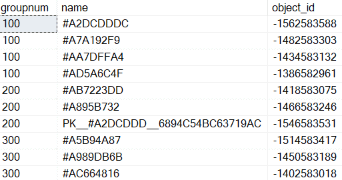
Report 6 shows the output when Listing 9 is executed. Note that the results will vary here except for the groupnum column.

Report 6: Output from Listing 9

Image showing results of sequence with minimum 100 and increment 100

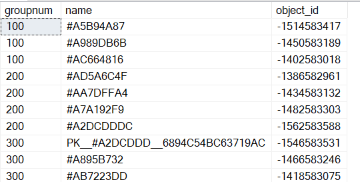
If the code in Listing 7 is run a second time, you will see the results shown in Report 7.I specifically only returned 10 rows in the subquery in Listing 9. I did this to show how the OVER clause associated with the NEXT VALUE FOR function might create grouping sets with different numbers of members. See how groupnum 100 has 4 rows, whereas each of the other groups only have 3 rows. This happened because the 10-row set of objects is not evenly divisible by 3.

Report 7: Second execution of Listing 9

An image showing the results of sequence starting at 100 and incrementing by 100. 200 repeated 4 times

In order to have the code produce exactly the same results each time, the sequence object used in conjunction with the OVER clause will need to be restarted. The code in Listing 10 uses the ALTER SEQUENCE command to restart the GroupBy3 sequence object then runs the same code as used in Listing 9.Now groupnum 200 has 4 rows. Why did this occur? This happened because the last sequence number value of 100 was stored in metadata when the Groupby3 function was used the first time. Therefore when Listing 8 was run a second time, the first group number generated was 200, and the last group number generated was 200. If Listing 9 runs a third time, you would see that groupnum 300 had 4 rows.

Listing 10: Restarting Sequence object to get consistent results

USE tempdb;
ALTER SEQUENCE GroupBy3
      RESTART WITH 100
      INCREMENT BY 100
          MINVALUE 100
          MAXVALUE 300
          CYCLE; 
GO
SELECT NEXT VALUE FOR GroupBy3 OVER (ORDER BY object_id) 
       as groupnum,name, object_id
FROM (SELECT top 10 name, object_id FROM sys.objects) AS O
ORDER BY groupnum;

By restarting the sequence number at 100 each time, the SELECT statement in Listing 10 produces exactly the same results each time it is run. I’ll leave it up to you to test out Listing 10 to verify that the code creates consistent results each time it is run.

The caching option

The CACHE option is available to reduce the amount of I/O that occurs when generating sequence numbers. When the CACHE option is enabled, information is stored in memory to reduce the amount of I/O written to the system metadata as sequence numbers are generated. The number of sequence numbers that can be generated without I/O to metadata is determined by the cache size.

Caching sequence numbers uses very little memory. Only two numbers are needed in memory to support caching, the last sequence number used and the number of values left in the cache. The size of those numbers is determined by the data type of the sequence object.

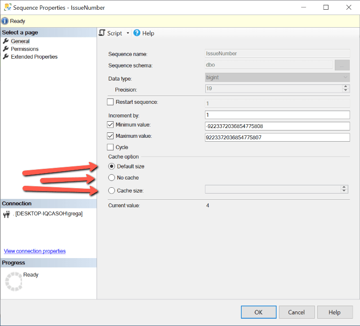
There are three different settings possible for the CACHE options. These three options can be seen by reviewing the IssueNumber sequence object using Object Explorer, as shown in Figure 1.

An images showing the sequence object properties

Figure 1: Sequence object IssueNumber specifications

The IssueNumber sequence object uses the Default size for the cache. The default size is not specified in the Microsoft documentation of sequence objects. The documentation says the default size for the CACHE option is determined by the Database Engine. It also states that the method for calculating the default size might change over time.

The second cache size option is No cache. When this option is specified, no memory is used to cache sequence values, and I/O will occur to the system metadata to maintain the last sequence number used each time a sequence number is generated.

The last option is Cache size, which uses memory to minimize I/O as new sequence numbers are generated. The constant associated with this option determines how many sequence numbers can be generated before the last generated sequence number is stored in the system metadata which uses I/O.

When SQL Server is stopped, the last sequence number generated in memory is written to the metadata so unused sequence numbers associated with the cache are not lost. Keep in mind that if SQL Server were to crash, this writing of the last sequence number would not happen, causing sequence numbers to be skipped. To understand more about how the Database manages the cache, refer to the Cache Management section in the Microsoft Documentation.

Expanding your knowledge of SQL Server sequence objects

The sequence object was introduced with the rollout of SQL Server 2012. Sequence objects can populate one or more columns in a single table and synchronize a series of generated numbers across multiple tables. Sequence objects provide more functionality for automatically generating numbers than an identity column. Next time you find identity columns don’t provide the features you need to generate a series of numbers, consider using the sequence object to see if it meets your auto-numbering requirements.


The post Using SQL Server sequence objects appeared first on Simple Talk.


from Simple Talk https://ift.tt/3CklhKM
via

Dependency Hell: Past and Future

Saying that I’m from the time of the MDAC would be to break the main rule of never reveal our age. However, who really remembers Microsoft Data Access ComponentsMDAC – today ?

Microsoft had ODBC and it was good. Out of the blue came Borland with a thing called BDE that was way faster and came with Delphi, a direct competitor of Visual Basic at that time. Microsoft had to be fast creating a new technology. That’s when MDAC was created.

Things were a bit crazy considering how fast MDAC was created. Windows brought one version of MDAC, lets suppose it was 2.1. Office and Access brought a different one, let’s suppose 2.3. SQL Server had 2.6 and Visual Basic 2.8. Of course the version numbers are not correct, this happened about 30 years ago, but you got the idea. It was craziness to understand what version was where.

Don’t know what was MDAC? What if I call it ADO, is it more familiar to you? Yes, I’m talking about ADO and it’s that old.


That was also the time of the big conferences. I was living in Rio and that was the first time I was getting a plane to attend Microsoft TechEd in São Paulo.

It’s difficult to compare that time with today. The speaker told us he was creating the demo scenario for the conference in the plane and noticed how difficult it was to update COM classes. He created an addIn for Visual Basic – still in the plane – unregister, compile and register the COM class again, that was a huge improvement in COM+ development and became part of the product less than a year later.
This same speaker addressed on the stage the problem of the multiple MDAC versions attached to different products. His sentence was something similar to this:

“We know the pain this caused to you, we know it was a mess. We will never release new versions this way again. New versions will only be released with the entire product”

After Some Years

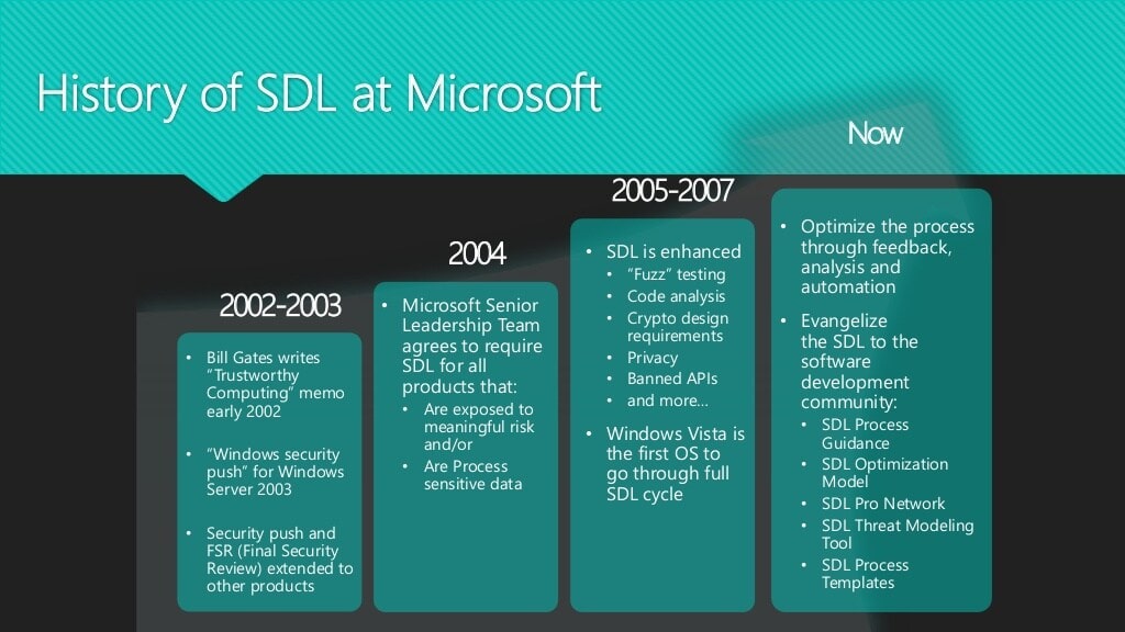
At some point in the end of 2001 and beginning of 2002 Microsoft suffered from some severe security problems on its products. The problem was so severe and exposed that Microsoft stopped all the software development during the entire month of February 2002, making every developer focus on security check of the code.

I hope not be mixing dates, but it was around this time I remember about a video explaining some pieces of the software development process in Microsoft. What most impressed me was the explanation that after a day of development, all the software was integrated, expend the entire night being tested and the developers had access to the result of the tests in the morning.

Having this level of automated tests, the possibility to leave small bugs behind would be low. Only hard to find ones would pass.

The image below, of course, is from many years ago.

The today World

Let’s talk about the today world based on examples.

LocationMode for Azure Storage access

LocationMode was a great property in the Azure Storage. The storage has replication by default and the LocationMode property allows you to use the replicated storage to balance workload with the primary storage, or other purposes.

You can see details about the LocationMode property on this page

The problem: The last version of the library with this property is the version 11 of the library. Version 12 of the library doesn’t have this property. A documentation page on Microsoft website says “We are working on producing documentation for this”, but the property is just no there.

Durable Functions

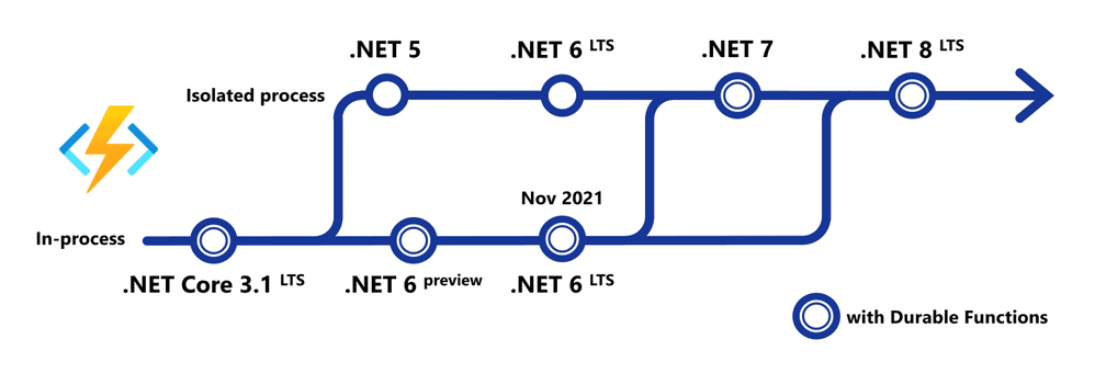
Durable functions allow us to create many different long running architectures using Azure Functions environment. The problem: only  .NET Core 3.1 LTS supports it. The .NET 5 or .NET 6 (until this month) don’t support it. There is one version of .NET 6 expected to become available this month that will make durable functions available again.

All this creates a problem: A version evolution is not a version evolution anymore. If we would like to enjoy the new version benefits we end up having to leave some feature behind. Is this something good?


It may worth read the following blog about LTS support and its meaning. I leave up to you to commend about the fact it resembles too much the name of Extended Support, becoming one more technical detail to learn and make everyone confuse.

System.Data.SqlClient and Microsoft.Data.SqlClient

Microsoft.Data.SqlClient is replacing System.Data.SqlClient, but it’s being made in a way that both live together, side by side. What are the chances for this to go wrong?

Microsoft.Data.SqlClient receives all new features implementations. For example, authentication with managed identities is supported only by this library. However, using this library isn’t the most straightforward process. A simple google query (sin! mortal sin!)  would show how easy it is to reach a dependency hell if you try to use it with .NET 5 in an Azure function. This blog is an example. Proposed solution? Downgrade .NET.

It’s not only about Development

SAS Policies on containers

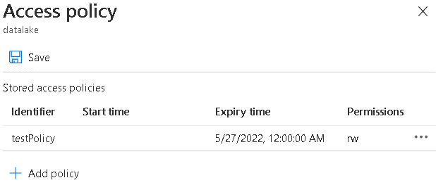
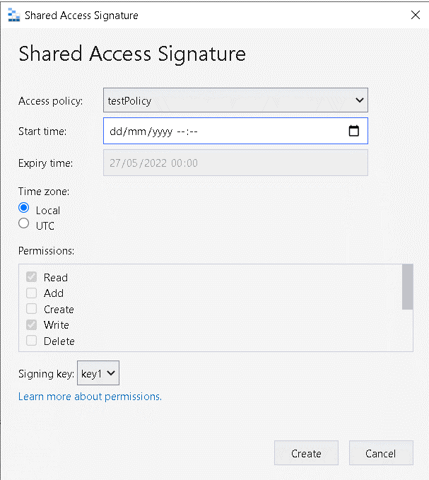
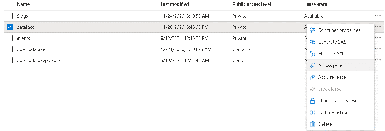
Do you know you can create a Shared Access Policy in an Azure container storage and this shared access policy should work as a guidance to produce SAS keys for the Azure Storage?


Yes, you can ! But no one knows, due to one simple reason: You can’t produce the SAS keys based on the SAS policy using the portal. Azure Storage Explorer can do this, but most people will miss and only look for the feature in the portal.


This plus the user being able to just ignore the SAS policy and create an SAS key in the way would like makes this feature… a bit strange.

The Hierarchical Namespace hell

In an Azure Storage account, we can enable Hierarchical Namespace or not. Can you correctly tell what features require Hierarchical Namespaces enabled and what features require it disable?


I know some features that require it disabled: Azure SQL Extended Events and temporary storage for backup restore are two of them. Things become even more strange when new features in Azure Storage, such as soft delete, only work with it disabled. What is this option for? Data Lakes. But Polybase and its flavors from Synapse and SQL can work well without this feature enabled. Confuse?

Conclusion

This list could be going and going. After finishing I may have thought about many more items that could figure here.

I don’t have answers, only questions. 30 years have passed, but does this justify that we go on the exactly opposite direction than the promised one in that conference in São Paulo? What about the night integration and tests, are they still happening ?

Young developers may hold pride for being able to walk through a dependency hell. Knowledge brings pride, but this knowledge shouldn’t, because in the end, it’s still a dependency hell.

Wouldn’t it be so easier if it just worked?

The post Dependency Hell: Past and Future appeared first on Simple Talk.


from Simple Talk https://ift.tt/3CnVtxn
via

Monday, November 8, 2021

SQL Elevated Configuration: The fail-safe for maintenance

Many years ago, in the company I was working for, one junior DBA started a reindex operation in a SQL Server Standard Edition on the most busy day of the month. Do I need to explain what happened next? It’s easy to use the imagination on this one.

What’s the option to solve this? Online index creation or rebuild. This would allow index maintenance to not block the database at all.

SQL Server 2019 and Azure SQL brought two database scoped configurations to work as a fail-safe for this kind of situation: Elevated_Online and Elavated_Resumable

Database Scoped Configurations are in some ways similar to server configurations, but we can set them on database level. On the beginning, they were server configurations we could set on the database level. After a while some configurations that work only as Database Scoped Configuration started to appear.

These two configuration options work as a fail-safe in case a junior DBA executes a statement that will block the server: When enabled, these configurations automatically convert the statements to online execution or resumable execution.

They are not enabled by default. I strongly recommend to enable them, avoiding blocking your production database when you less expect.

Managing the Configurations

You can check if these statements are enabled using the following query:

SELECT *
FROM   sys.database_scoped_configurations
WHERE  NAME IN ( ‘ELEVATE_ONLINE’, ‘ELEVATE_RESUMABLE’ ) 


These options are not a simple ON/OFF switch. They have 3 configuration options:

OFF: It’s the default. The configuration is disabled.

WHEN_SUPPORTED: It’s the one I most recommend. SQL Server will change the statement to online/resumable when possible, but if for some reason it’s not possible, the statement will be executed anyway.

FAIL_UNSUPPORTED: This is the most strict option. The execution will fail If for some reason the statement can’t run online. I recommend to be very careful when using this option. If we could set time windows for this option, defining when the statement can or can’t be executed, it would be way better.

Example to set these configurations:

ALTER DATABASE SCOPED CONFIGURATION SET ELEVATE_ONLINE = WHEN_SUPPORTED;
ALTER DATABASE SCOPED CONFIGURATION SET ELEVATE_RESUMABLE = WHEN_SUPPORTED;

Recommendation for Production Environments

In critical production environments, one option is to keep both configurations set with FAIL_UNSUPPORTED. Every maintenance requiring to execute something offline or not resumable would need to change the configuration first, make the execution and revert the change.

The first security blocking production issues is that someone who wants to execute a dangerous task for production will need to be aware about this configuration and really know what to do.

We can add one more security level using permission management. In order to change a database scoped configuration the user needs the ALTER ANY DATABASE SCOPED CONFIGURATION permission. The server administrator will need to manage permissions in such a way that only a limited set of administrators will have these permissions, while junior administrators will have limited permissions to manage the database.


The post SQL Elevated Configuration: The fail-safe for maintenance appeared first on Simple Talk.


from Simple Talk https://ift.tt/3mSEZZU
via

Wednesday, November 3, 2021

SQL Server 2022 is a game changer

Microsoft announced at the Ignite conference that SQL Server 2022 is on the way, and several significant new features should convince many organizations to upgrade soon after it’s available. It’s been three long years since SQL Server 2019 arrived, so these announcements are exciting to hear.

Microsoft will announce details and additional features over the next few months, but to see demos of the announcements from Ignite, take a look at this video from Bob Ward. Microsoft is also presenting deep dive sessions of all the features at the PASS Data Community Summit, November 8 – 12. If you register before the keynote on November 12th, you will receive exclusive access to the session recordings for six months, so don’t wait. Sign up today!

Here are the two features that I’m looking forward to trying:

Failover to Azure SQL Managed Instance

With just a couple of clicks, you can attach a database to the cloud. This action sets up an Availability Group (AG) between an on-premises SQL Server and Azure SQL Managed Instance (MI), which you can use for disaster recovery or offloading a read-only workload. You can then manually failover to the MI and back. It’s also possible to restore a backup from a MI to SQL Server 2022.

Instead of managing hardware or virtual machines in multiple data centers, you can let Microsoft do the work for you with Azure SQL Managed Instances saving money, effort, and time.

Parameter sensitive plan optimization

Beginning with SQL Server 2022, multiple plans can be cached for a query. If there are two possible plans for a query, the plan will switch between a scan and a seek depending on the number of rows processed. This new feature solves those pesky parameter sniffing issues that cause so many performance issues. I’ve been hoping to see this improvement for years and can’t wait to see what else is in store.

Microsoft also announced Azure Synapse Link with SQL Server for real-time analytics without ETL, Azure Purview Integration, SQL Server Ledger for data tampering protection, and much more. Don’t miss all of the announcements and demos of the new features at PASS Data Community Summit.

SQL Server is a game-changer with something for everyone. I can’t wait to get my hands on the preview!

Commentary Competition

Enjoyed the topic? Have a relevant anecdote? Disagree with the author? Leave your two cents on this post in the comments below, and our favourite response will win a $50 Amazon gift card. The competition closes two weeks from the date of publication, and the winner will be announced in the next Simple Talk newsletter.

The post SQL Server 2022 is a game changer appeared first on Simple Talk.


from Simple Talk https://ift.tt/2ZKp7PY
via

Tuesday, November 2, 2021

Ransomware: A world under threat

Ransomware represents one of the biggest security threats faced by today’s organizations. A ransomware attack can have a devastating impact on an organization, and few organizations are immune from the threat. It doesn’t matter the organization’s size, type, or location. It could be a university, city government, school district, small business, private corporation, or another type of institution. Any entity whose operations rely on computers and the flow of data is at risk from a ransomware attack, and if the attack is successful, it could cost the organization millions, whether or not the ransom is paid.

What is ransomware?

Ransomware is a form of malware that prevents organizations from accessing their data or systems. Threat actors who carry out ransomware attacks hold the data or systems hostage until a ransom is paid. Individuals can also be hit with ransomware, but most crooks are looking for bigger payoffs, and those come from public and private organizations, especially those that rely heavily on their data to carry out day-to-day operations. A ransomware attack can, in fact, bring an organization to its knees, preventing it from conducting business and often leading to the loss of critical data.

Ransomware attacks vary substantially from one to the next and are continuously evolving. They range in scope, types of targets, and amounts of ransoms they demand. Even so, they generally follow similar steps:

  1. Threat actors use an attack vector to gain access to a target system or network, where they introduce the ransomware. Common attack vectors include phishing, spear phishing, malvertising, malicious websites, stolen credentials, and social engineering campaigns. Ransomware can also be introduced through the use of other malware.
  2. After the ransomware penetrates a system, it carries out whatever operations it was designed to do, often spreading to other nodes on the network. Threat actors might introduce ransomware that exploits known vulnerabilities in order to gain access to restricted resources, or they might use social engineering techniques in conjunction with ransomware to get to these resources. Most ransomware either locks up computers or encrypts files. However, attacks against organizations commonly use encryption. In most cases, ransomware victims are not aware of an attack until it’s too late.
  3. Once the ransomware has taken control of the data or systems, the threat actors make their ransom demands known to the victim. For example, if the ransomware has encrypted sensitive data, the threat actors might demand that the victim make a payment in the form of cryptocurrency (such as Bitcoin). In exchange, the victim will receive the decryption key. If the victim does not make the payment within the deadline, the threat actors might demand a higher ransom. If the victim refuses to pay the ransom altogether, the data will never be decrypted.

When planning their ransomware attacks, threat actors often carry out extensive research on the target organizations, discovering what they can about their financial circumstances, the types of regulations that govern their data, what it could cost them to have their data locked, and any other information that might be useful when making their ransom demands. It cannot be overemphasized how sophisticated ransomware attacks have become and the planning and research that often go in them.

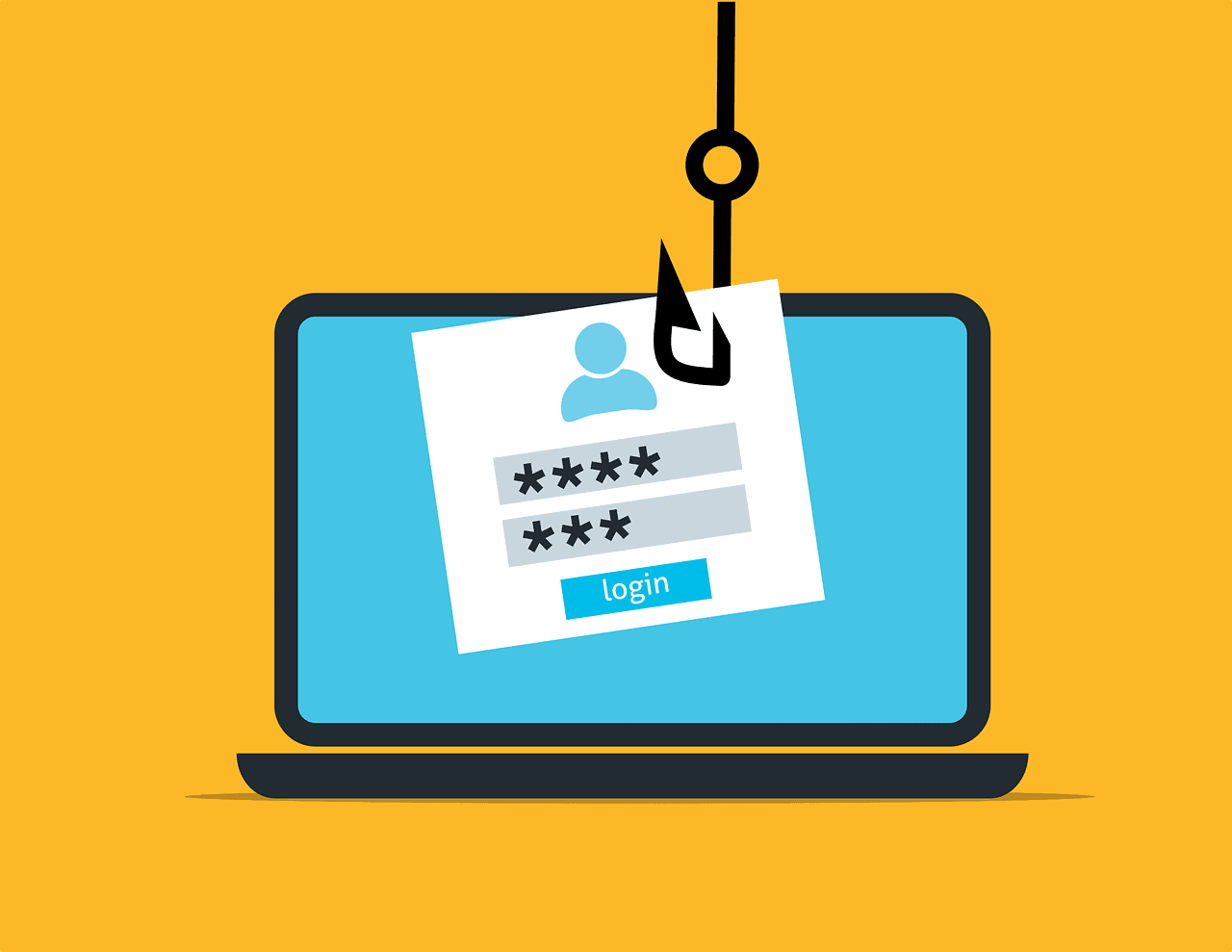
An image representing a phishing attack

Figure 1. Threat actors commonly use phishing to introduce ransomware into a target system (image by Mohamed Hassan).

In the early days of ransomware, attacks primarily targeted individual users, and although this still occurs, threat actors have come to realize that they can make a lot more money by going after organizations—disrupting their business and threatening their data.

Organizations large and small are at risk from ransomware. In some cases, threat actors might launch an attack against an organization because it appears easier to infiltrate and control, such as a school district with a limited IT budget, or they might take on organizations that seems more likely to pay, such a hospital that relies on continuous access to patient data. In recent years, universities, financial institutions, and healthcare organizations have been hit particularly hard by ransomware.

Ransomware’s insidious spread

A number of factors have helped fuel the rise in ransomware. One of the most important was the introduction of cryptocurrency, which facilitated anonymous payments and made it difficult to prosecute the criminals who launched the attacks. The dark web has also played an important role by providing threat actors with resources for carrying out their attacks. Would-be attackers can surf ransomware marketplaces, purchase malware kits, or find developers who sell ransomware as a service (RaaS), which offers ransomware for a cut of the take.

It’s no surprise that threat actors are drawn to ransomware, given the ease of getting into the business and the potential big pay-offs, and in such a climate, ransomware attacks are likely to grow more sophisticated and aggressive. According to the Sophos State of Ransomware 2021 report, which is based on the company’s annual ransomware survey, 37% of the surveyed organizations were hit by ransomware in the last year—over one-third of the 5,400 surveyed. The report also includes other notable findings:

  • Mid-sized organizations paid an average ransom of US$170,404.
  • The total costs of a ransomware attack averaged US$1.85 million, when taking into account ransom payments, downtime, personnel time, device and network costs, lost opportunity, and other factors.
  • Of those organizations that suffered a ransomware attack, 54% stated that the cybercriminals succeeded in encrypting their data in the most significant attack.
  • Of these organizations, 96% got their data back, but only 65% of the encrypted data was restored after the ransom was paid.
  • Extortion-style attacks more than doubled in the last year, up from 3% to 7%. In these attacks, cybercriminals threatened to publish the data, rather than encrypting it. It should also be noted, however, that threat actors have started to carry out double-extortion attacks in which they steal and encrypt the data and threaten to publish it online.

The rate of attacks is actually down from the previous year, when 51% of the surveyed organizations stated that they had been hit, but the drop might be due in part to evolving attack approaches, according to the Sophos report. “For instance, many attackers have moved from larger scale, generic, automated attacks to more targeted attacks that include human operated, hands-on-keyboard hacking. While the overall number of attacks is lower, our experience shows that the potential for damage from these targeted attacks is much higher.”

An image that represents ransomware

Figure 2. Ransomware attacks continue to grow more sophisticated, targeted, and aggressive (image by Katie White).

The first recognized instances of ransomware occurred in the 1980s, but it wasn’t until the 2000s that modern forms of ransomware started to appear. Initially, such attacks were confined mostly to Russia, but the picture changed dramatically by 2012, when ransomware attacks proliferated and spread across the globe. This was in large part because of the emergence of Bitcoin, which provided an anonymous platform for receiving ransom payments.

Since then, ransomware has become one of the most dominant forces in the threat landscape, producing a wide range of variants, including the following:

  • CryptoLocker. A highly powerful form of malware that first emerged in 2013 and set the stage for the type of ransomware that encrypts files on hard drives and connected devices, spreading much easier than earlier variants.
  • WannaCry. One of the most well-known and damaging types of ransomware to hit cyberspace. WannaCry leveraged EternalBlue, a Windows exploit allegedly developed by the US National Security Agency (NSA) and then stolen by a group of hackers known as Shadow Brokers. The NotPetya ransomware also used the EternalBlue exploit.
  • SamSam. Ransomware that exploits server vulnerabilities to gain access to a network, where it lingers undetected for long periods of time. Attackers have often used the Remote Desktop Protocol (RDP) in conjunction with SamSam to infiltrate the network and search for valuable targets. One of the most notable SamSam attacks occurred in 2018 against the city of Atlanta, Georgia, which spent over $2.6 million to recover from the incident.
  • Ryuk. Ransomware often used along with other malware (such as the TrickBot banking Trojan) to infect vulnerable or high-profile targets. Ryuk emerged in 2018 and has since wreaked havoc on news agencies, healthcare organizations, school systems, and other institutions. According to the CrowdStrike 2020 Global Threat Report, Ryuk accounted for three of the top seven ransom demands for that year: USD $5.3 million, $9.9 million, and $12.5 million.
  • Egregor. Malware first identified in September 2020 that was once considered a high-severity threat until US and Ukraine authorities worked together to stop operations. Despite its demise, Egregor represented two significant ransomware trends: RaaS and the double extortion attack.

There are plenty of other examples of ransomware out there, and there are a growing number of examples of its consequences. Earlier this year, for instance, Colonial Pipeline fell victim to a major ransomware attack, causing the company to shut down its fuel distribution operations. Not only did this lead to widespread fuel shortages, but it also resulted in personal information being compromised. Colonial Pipeline paid $4.4 million in ransom for the decryption key.

Protecting against ransomware

According to prevailing wisdom, the best way to protect against ransomware is to prevent it from happening in the first place. This is no doubt true enough, but implementing these protections can be a significant undertaking, even under the best circumstances. That said, IT and security teams have no choice. They must be aggressive in the steps they take to protect their systems and data while at the same time, prepare for how to respond to a ransomware attack if one occurs.

To protect against ransomware and other security risks, an organization needs to employ a defense-in-depth strategy that takes a multi-layer approach to security. Not only can this help to protect against different types of threats, including ransomware, but it can also minimize the impact of an attack if it should occur. Such an approach requires careful planning that takes into account ransomware protections. To this end, here are four general guidelines to consider when mapping out your security strategy:

  1. Create secure backups. Backups are your best protection against ransomware, but the backups themselves must also be safeguarded. They should be secured with the strictest protections, and at least one copy of each backup should be immutable and disconnected from the computers and networks that you’re backing up. You should also verify that your backups are complete and viable, and you should regularly test your restoration process.
  2. Secure your environment. This is a broad category that is typically part of a larger security strategy. It includes the use of security software that includes ransomware protection, and it incorporates other best practices, such as keeping all software updated and patched, controlling which applications users can install, performing regular vulnerability scans, maintaining strong access controls, using multi-factor authentication (MFA), implementing robust email security, running penetration tests, and continuously monitoring your environment for malicious activity.
  3. Train and educate personnel. An organization should have in place an awareness and training program that educates users in how to avoid ransomware and other threats. The better they understand the threat landscape, the less likely they’ll be to carry out risky behavior. For example, they should be trained in how to safely surf the web and what to do if they receive suspicious emails. IT and security teams should also receive the training they need to stay current on ransomware threats and what steps to take to best mitigate risks.
  4. Create an incident recovery plan. Regardless of how diligent an organization might be when it comes to security, no one is completely free from risk. The organization should implement an incident recovery plan that defines the roles, responsibilities, and procedures to follow when responding to a ransomware attack. The plan should also include a list of individuals and organizations to contact in the event of an attack. In addition, it should identify critical processes that need to continue uninterrupted if an attack occurs and what it will take to maintain operations without access to certain systems. IT and security teams should also practice their incident responses to ensure a smooth operation in the event of a real attack.

If a ransomware attack were to occur, an organization would immediately implement its incident recovery plan. In most cases, the first step would be to identify and isolate the infected devices to stop the spread as quickly as possible. If the devices can’t be disconnected from the network, they should be powered down, but this should be a last resort to avoid losing forensic evidence.

The response team should also report the incident to the appropriate law enforcement and regulatory agencies and to any key players that need to be informed of the attack. The team should then fully investigate the incident, taking such steps as identifying the ransomware and assessing the damage. Once they understand the full extent of the attack, they can take the steps necessary to recover their data from the backups.

The continuous threat of ransomware

When organizations are victims of ransomware attacks, the question always arises of whether they should pay the ransom. Law enforcement agencies such as the FBI generally advise against paying. One reason for this is that the attackers might never provide the decryption key. And even if organizations pay, they might be targeted again by the same attackers or gain a reputation as susceptible targets. Some would also argue that paying the ransom only encourages more such attacks. Even so, many organizations pay the ransom anyway, seeing it as a better option than losing all their data, especially if they cannot operate without that data.

Whether or not they pay, ransomware is here to stay. It will continue to evolve, and attacks will become more sophisticated and targeted. It might not be long before criminals move from computers and data to critical infrastructure, such as smart cities or industrial control systems, hijacking an entire ecosystem until the ransom is paid. Yet even in its current form, ransomware represents a significant threat to both public and private sectors, targeting organizations at all levels. Only by taking steps to protect against ransomware and to prepare for a possible attack can organizations hope to avoid or minimize the potential havoc that ransomware can wreak.


The post Ransomware: A world under threat appeared first on Simple Talk.


from Simple Talk https://ift.tt/3Bwf2mN
via

Monday, November 1, 2021

Data Factory: Use a SQL Query to create a Data Source

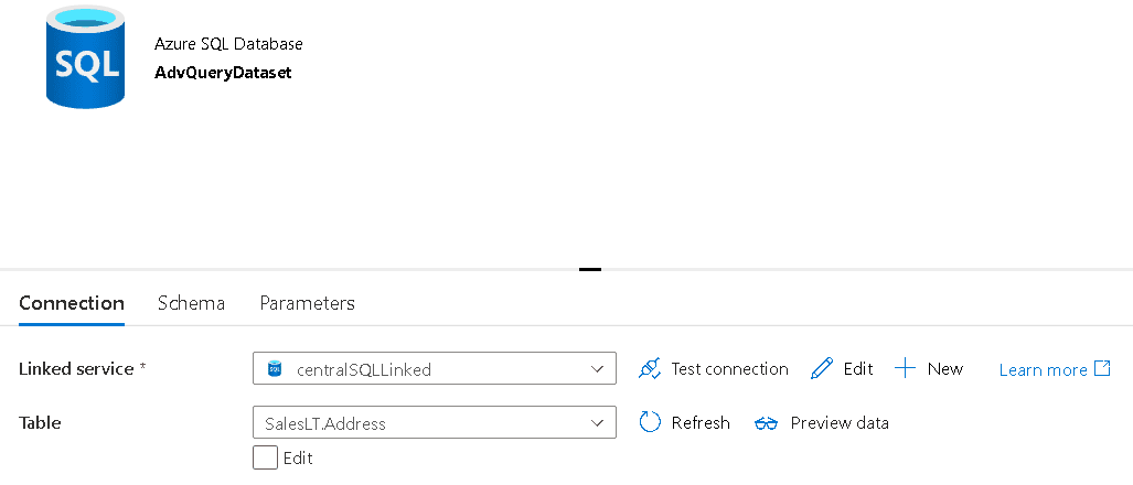
When we include a data source inside a data flow it always requests a dataset. The dataset, in turn, requires you to point to a table. A dataset can’t be defined over a query, it needs an object on the linked service, which may be a table or view as you may notice on the image below.


How can we work around this and use a query as a source for a data flow?

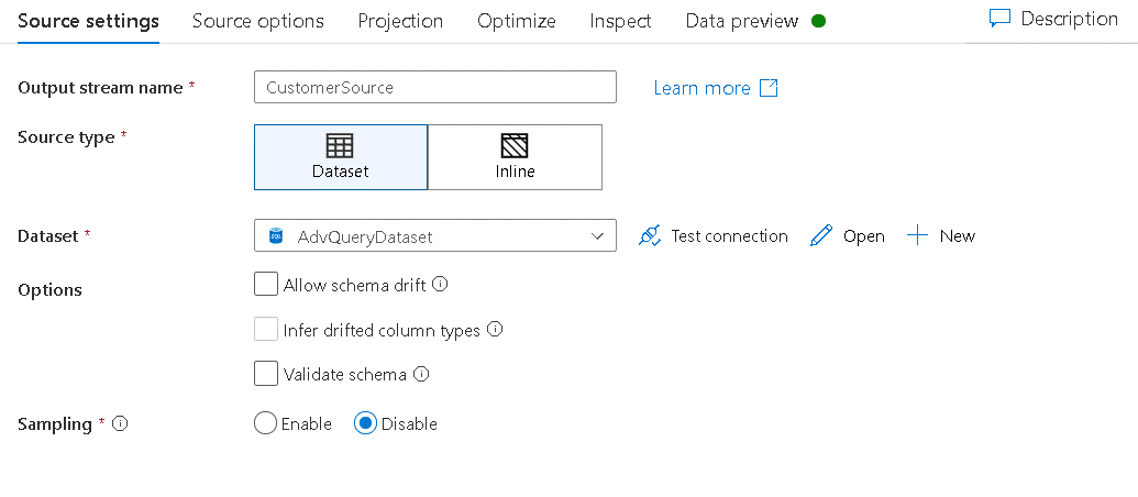
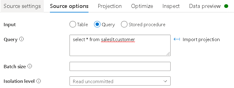
The secret is on the source object we use on the data flow. We need to select a dataset, as always. However, on the 2nd tab, Source Options, we can choose the input type as Query and define a SQL query. The source will ignore the table configuration in the dataset and get the data from the query.

This is how the 1st tab will look like when we select the dataset:

This is how the 2nd tab looks like with the query defined:


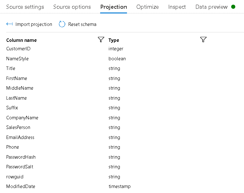
After defining the query, we can click the button Import Projection. Data Factory will need to initialize the Integration Runtime, so it can execute the import of the schema. Once the Integration Runtime is initialized, the Import Projection can proceed. Usually you will need to click the button again.

On the Projection tab we will not see anything related to the table at all, only the query results will be there.


The schema drift properties on this scenario are still optional. They will act completely over the query. We import the projection schema from the query. The dataflow will accept additional fields beyond the ones defined during development if the schema drift property is enabled, as it usually does.

The Dataflow Code

We can say in some ways the data factory data flows have two different languages: The Data Flow Script (DFS) and the json syntax. The two buttons on the top right of the Data Factory screen allow us to see the code.

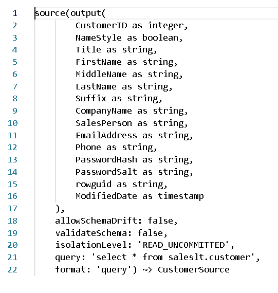
The DFS from this script makes no reference to the dataset at all:

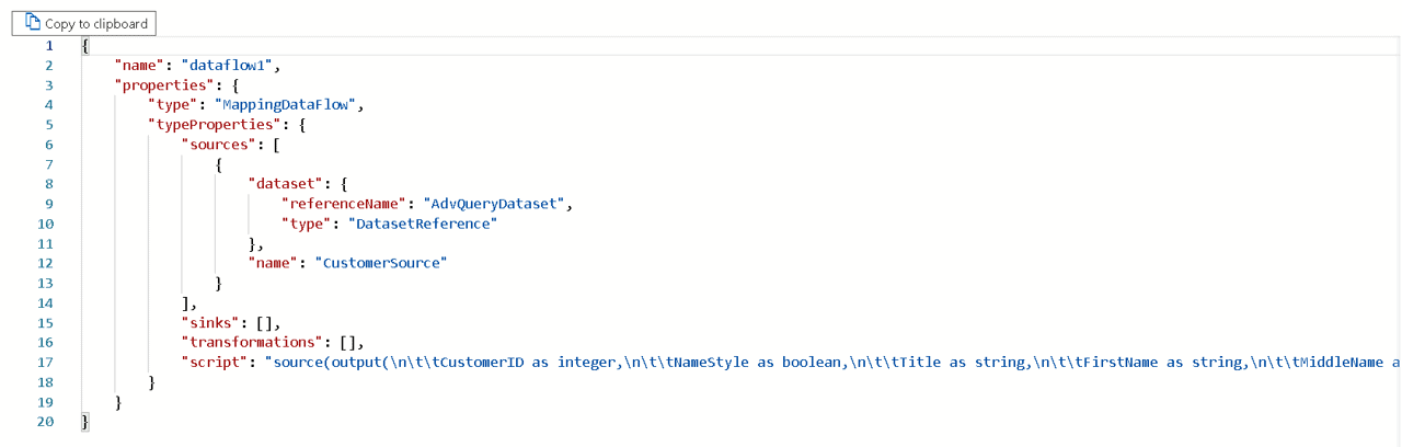
Data Factory converts the DFS to a single script line in the JSON file. The JSON file requires a source dataset specified, but many dataset definitions, such as the table, will be ignored. The resulting JSON will be like the image below.

The dataset, on this example, establishes a link between the data flow and the linked service, but only that.

The post Data Factory: Use a SQL Query to create a Data Source appeared first on Simple Talk.


from Simple Talk https://ift.tt/2ZHfCBC
via