Wednesday, November 24, 2021

Working with PowerShell strings

One of the things that I’ve both appreciated about PowerShell but also been at times confused by PowerShell is its concepts of strings and variables. This article explains what you need to know when working with PowerShell strings.

For example, when you start writing in PowerShell, you may notice that you can use single quotes or double quotes to designate a string.

Starting simple

"A very simple string."
$string1 = "This is a string variable."
$string2 = 'This is also a string variable.'
$string1, $string2
write-host $string1, $string2
write-host $string1 $string2

Save the above as SimpleStrings_demo.ps1. And as usual, examples are available at Github.

When you run the above, you will see the following output:

Image showing output of script. Sometimes, there is a new line

The first line is echoed as is because you haven’t told PowerShell to do anything special.

Then you have created two variables and assigned strings to them. Again, in the case where there’s no assignment and no cmdlet used, PowerShell simply echos out the contents of the variables, one to a line.

When you use the write-host variable, PowerShell will again write them out, but this time keep them on the same line. It doesn’t matter here if you use a comma or not to separate them.

So far, the strings with double quotes and single quotes act the same way. But there is a difference which you’ll see in the following example:

$name = "Greg"
$age = 53
"My name is $name and my age is $age."
$string1 = "DQ: My name is $name and my age is $age."
$string2 = 'SQ: My name is $name and my age is $age.'
write-host $string1
write-host $string2

Save the above as SimpleStrings_with_variables_demo.ps1 and run it.

Your output will look like:

Image showing that variable not replaced in single-quote string

You will immediately notice that in the case of the double quotes, PowerShell did replace the inline variables of $name and $age with their values. However, in the case of single quotes, it treated the variables as part of the string itself and did not replace them.

The upside is that it’s very easy to write out strings with the value of the variables embedded directly in the string. The downside is that you can’t easily print out the variable’s name, which you may want to do while debugging a script.

The following example, SimpleStrings_with_variables_demo_2.ps1 shows a few ways of solving that problem:

$name = "Greg"
$age = 53
"My name is $name and my age is $age."
$string1 = "The `$name value is $name and the `$age value is $age."
$string2 = 'The $name value is ' + $name + ' and the $age value is ' + $age
$string3 = 'The $name value is ' + $name + " and the `$age value is $age"
write-host $string1
write-host $string2
write-host $string3

Image showing other ways to add variable to string

You will notice the backtick character ` allows you to escape the $ so that PowerShell does not treat the characters that follow as a variable name. That is generally the way I do it.

You may be tempted, and it’s perfectly legal, to build a string as shown in $string2, however, I find that harder to read and more complex and see no value to it. $string3 is simply an example showing you can use both single-quoted strings and double-quoted strings when building up a larger string. However, I would definitely avoid that one.

Dealing with objects

You will often find yourself dealing with objects when working with PowerShell. Dealing with objects introduces an issue, but fortunately, like most things, PowerShell has a solution. The following examples can be found in the Github repository in the file Strings_with_object.ps1.

Start by creating an object. For the purposes of this demo, it will be a simple instantiation and assignment.

$person1= @{Name='Greg' 
Age=53}

This object has two properties: a name and an age. Again if you simply hand the object to PowerShell and execute it, PowerShell will print something out, but a bit differently from the above examples.

Pass $person1 to PowerShell and hit enter, and you should see something like:

Image showing tabular results

This method is not terrible, but also not terribly useful. However, if you try to use the write-host cmdlet as follows: write-host $person1, you don’t get what you might expect. Instead, you get the curious response of:

Image showing that printing object shows type not value

That’s not overly helpful. If you try to put the object in between double quotes (since you know with single quotes, it will simply print out what it is handed), you will get the following:

write-host "This is all about $person1"

Image showing that adding $ to object name doesn't print value inside a string

Note the difference in the two responses. In the first case, PowerShell is attempting to parse the object and determine two properties within the object. In the second case, PowerShell doesn’t do any parsing but simply determines it is a hashtable.

The above responses provide the clues you need to get what you want. But before you get there, try the following:

$person1.Name, $person1.Age

You will get:

Image showing you can print object property

This result makes sense because now you are specifying which property you want, but it’s still far from perfect.

You may try the following, which seems like it should work:

write-host "This is all about $person1.Name"

But, curiously, this fails with the following:

Image showing that object variable with property is not replaced in string

Note that this message is a bit different from the above one that mentioned this being a Hashtable. It has .Name appended to the end. It appears that PowerShell is correctly trying to expand the object, but it’s ignoring your reference to a specific property.

The solution here is to force PowerShell to evaluate the entire object before it gets to Write-Host.

You may be tempted to try the following:

# A work around
$personName = $person1.Name
write-host "This is all about $personName"

Executing this will work:

image showing the results of a work around

But, it’s wordy and, in my opinion, a bit messy. Imagine you had an object with a dozen or more properties you wanted to write out.

The solution is to take advantage of scoping and to use parentheses as follows:

write-host "This is all about $($person1.Name) who is $($person1.Age)"

This code will return:

Image showing the result of using parentheses

This result is most likely what you wanted. PowerShell starts with the object inside the parentheses (e.g. $person1.Name) and evaluates that, and then treats it as a variable denoted by the outer $. Write-host then evaluates that variable and inserts it into the string.

Note this means you can do some additional fancy things such as the following

$person2 = @{Name="Joe"
Age=78}
write-host "Together $($person1.Name) and $($person2.Name) are a total of $($person1.Age + $person2.Age) years old."

This will produce:

Image showing summation of values from object

The summation of the ages of $person1 and $person2 happens before Write-host evaluates the outer $.

Formatting strings

Imagine you are tasked with using PowerShell to print out invoices from an order management system. With your newfound knowledge, you sit down and write something like:

$cost = 144.56
$quantity = 11
Write-host "Your cost for $quantity will be: $($cost*$quantity)"

Your output looks like:

Image showing output, cost for 11

It’s not quite perfect. You’d really like to include a currency character to the string, but you can come back to that later.

The more immediate issue is that when $quantity = 10. Then you get the following:

Note the missing trailing 0.

This problem is fortunately easy to fix. PowerShell strings allow formatting using .NET standards.

One simple way of fixing the above is the code below:

$formatted = "Your cost for {0} will be: {1:f2}" -f $quantity, $($quantity*$cost)
write-host $formatted

This will print:

That’s an improvement. The f2 is an instruction to return 2 floating-point values after the period. Additionally, you may want to put a currency symbol in there and a comma.

A simple fix would simply to do the following:

$formatted = "Your cost for {0} will be: `${1:n2}" -f $quantity, $($quantity*$cost)
write-host $formatted

Image showing output with $

Note two essential parts here. The dollar sign was added with a backtick ` so PowerShell doesn’t interpret it as the start of a variable name. In addition, by changing the f to n, PowerShell will treat this as a number using a cultural separator. This code will work equally well in a machine set up in Europe, where they tend to reverse the use of the period and comma separators. However, the currency character is still an issue which can be fixed with slightly different formatting:

$formatted = "Your cost for {0} will be: {1:c2}" -f $quantity, $($quantity*$cost)
write-host $formatted

Image showing output with currency symbol

Note that the $ is no longer needed as part of the string.

PowerShell isn’t just limited to formatting currency; you can use it for other formats. For example, say you needed to generate a list of User IDs with a specific format:

1..15 | % { 'UserID_{0:d4}' -f $_ }

The above will generate 15 User IDs of the format:
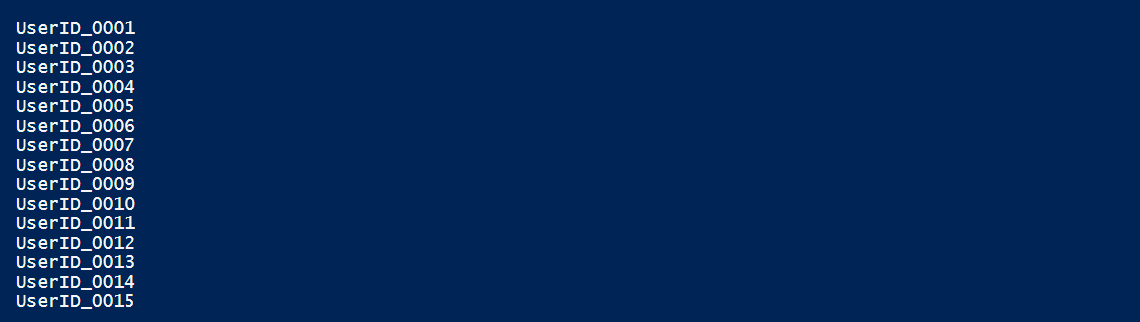
Image showing 15 user ids generated

A common requirement is formatting dates. There’s a couple of ways of doing this. If you do nothing and simply accept the defaults as follows:

$exampledate = get-date
write-host $exampledate

The results depend on your regional settings. In the US, you will get:

Image showing date and time

You could format the date when you create it:

$fdate = get-date -Format "yyyy-MM-dd"
write-host $fdate

This will return:

Image showing date only

Unfortunately, the variable $fdate contains only the information shown. You can’t later reference the time if you want.

However, there are a lot of built-in formats available:

$fdate = get-date -Format "R"
write-host $fdate

This method returns:

Image showing date with special formatting

If you want to store the full value of the returned date and later use only a formatted portion of it, you can do something like the following:

write-host $exampledate.ToString('yyyy-MM-dd')
Write-Host $exampledate.ToString("hh:mm:ss")

As you can see, there are plenty of ways to format your strings, dates, and other variables.

String padding and trimming

Often you may find yourself wanting to pad out or trim a string. You may want items to appear clearly in columns on the screen, or you may write to a file with fixed-length fields.

This task can be easily handled, as seen in the examples below. Save these as String_Padding_and_Trimming.ps1.

First, you need to generate some strings. Note that while the first variable claims to have three characters, it actually has a trailing space. This might go unnoticed in some cases if the value was read in from a database field.

$3char = "123 "  # note space!
$4char = "4567"
write-host $3char
Write-Host $4char

This looks perfectly fine as is:

Image showing numbers don't line up on right

# But what if we want them to line up, and we expect someday we might even have longer strings.
$padamount = 5
$padcharacter = ' '
write-host $3char.PadLeft($padamount,$padcharacter)
Write-Host $4char.PadLeft($padamount,$padcharacter)

This now almost works, but that trailing space is obvious:

Image showing numbers don't line up because of trailing space

Fortunately, this is fairly easy to fix using the trim() method:

write-host $3char.trim().PadLeft($padamount,$padcharacter)
Write-Host $4char.PadLeft($padamount,$padcharacter)

Image showing that using trim will align numbers on right

You can also pad to the right and, of course, select other characters. Again notice the trailing space is an issue, so in the second example, you can eliminate it.

$padamount = 7
$padcharacter = '.'
write-host $3char.PadRight($padamount,$padcharacter)
Write-Host $4char.PadRight($padamount,$padcharacter)

Image showing dots with numbers to show where the trailing space is

write-host $3char.trim().PadRight($padamount,$padcharacter)
Write-Host $4char.PadRight($padamount,$padcharacter)

You can do a lot more with the Pad and Trim methods once you fully understand them.

Adding some color to your life

Finally, what is life without some color, or, in this case, showing strings with color?

Like most things, PowerShell makes this very easy. Below is a script that was possibly written by a Hobbit to keep track of something near and dear to their stomach.

Save the following script as String_Color.ps1.

$tod = get-date
if ($tod.Hour -ge 6 -and $tod.Hour -lt 9)
    {
        write-host "Time for Breakfast!" -ForegroundColor Yellow
    }
elseif ($tod.Hour -ge 9 -and $tod.Hour -lt 11)
    {
        write-host "Time for 2nd Breakfast!" -ForegroundColor Red -BackgroundColor Green
        write-host "That's only if he knows about second breakfast!"           
    }    
elseif ($tod.Hour -ge 11 -and $tod.Hour -lt 12)
    {
        write-host "Elevenses!" -BackgroundColor Red
    }    
elseif ($tod.Hour -ge 12 -and $tod.Hour -lt 14)
    {
        write-host "Luncheon" -ForegroundColor Red -BackgroundColor Yellow
    }
else
    {
        Write-host "Afternoon Tea - 2:00 PM until 5:00 PM " -ForegroundColor Black -BackgroundColor DarkRed -NoNewline
        Write-host "Dinner - 7:00 PM until 9:00 PM " -ForegroundColor Red -BackgroundColor DarkBlue -NoNewline
        Write-host "Supper - 9:00 PM until 11:00 PM " -ForegroundColor Red -BackgroundColor DarkGreen
    }

The above script will help any Hobbit keep track of what meal they should be planning for. Note that portion control in case 12 dwarves show up unexpectedly is not covered.

If it’s early in the day, the script will simply change the foreground color of the text to yellow. This color change is done merely by adding the –foreground parameter to write-host.

In the case of second breakfast, you can set both the foreground and background colors as you desire. You will also note that any color you set is only in effect for that particular write-host cmdlet. The following one will revert back to the host colors in your terminal or IDE.

You can, as demonstrated with Elevenses, set only the background color.

Finally, if you want to have multiple colors on the same line, you can take advantage of the –NoNewLine parameter for Write-Host and suppress adding a newline character to your output. This technique can be useful if you want to build a menu option such as below: (save as Select_Option_With_Color.ps1)

write-host "1) " -ForegroundColor Red -NoNewline
write-host "select Option 1" -ForegroundColor Yellow
write-host "2) " -ForegroundColor Red -NoNewline
write-host "select Option 2" -ForegroundColor Yellow
write-host "3) " -ForegroundColor Red -NoNewline
write-host "select Option 3" -ForegroundColor Yellow
$result = Read-host "Select an option above"
if ($result -ge 1 -and $result -le 3)
    { Write-host "Thank you for selecting $result" }
else
    { "You selected an invalid value $result" }

PowerShell strings

In general, string handling in PowerShell is quite simple, but minor differences such as using double quotes or single quotes can make a difference. In addition, knowing how to escape a character or force the evaluation of a variable inside a string can make life simpler as you don’t need to add additional steps before you can output your string.

Additionally, most of the string operations shown in the article can be used when outputting to a file, making the creation of a CSV or file based on length delimited columns far easier to create.

If you like this article, you might also like PowerShell editors and environments part 2.

The post Working with PowerShell strings appeared first on Simple Talk.


from Simple Talk https://ift.tt/3cKsqtH
via

Tuesday, November 23, 2021

Connecting to PostgreSQL: Learning PostgreSQL with Grant

There was a time when most of us worked on a single data platform. Even today, many of us can easily say that we spend the majority of our time on one data platform. However, more of us are moving to manage or develop on, multiple data platforms. I’m right there with you. I have to support and understand many different platforms now. The one I’ve been working with the most is PostgreSQL. Yet, I don’t really feel like I know it very well at all. 

That’s going to change.

I’m going to go on a deeper dive into the PostgreSQL database and bring you along the journey with me. It’s not enough to be able to write a SQL script that works in PostgreSQL. Instead, I want to be able to perform real management, from backups to troubleshooting. Further, I want to develop a database there, with tables, keys, procedures, and all the rest. Finally, I want to be able to monitor and performance tune the queries in PostgreSQL.

That’s the plan.

Now, am I going to go so far as to start writing books on the topic?

No.

However, as I figure things out, I am going to write these blog posts so they can act as a learning guide for others.

If anyone has suggestions, questions, or any feedback at all, please, don’t hesitate to reach out.

Running PostgreSQL

In these wonderful modern times, you really don’t need to install software. Containers and database as a service offerings allow skipping that whole mess. However, if you do want to run PostgreSQL as a service locally, you will need to download PostgreSQL.

Pick the appropriate OS, and then you can download and run the install. Obviously, you can use Chocolatey, HomeBrew, or some other utility for a command line install.

Once you have it installed, you will need to start the service. I’m running Windows 11 at the moment, so I used the following command from a terminal window:

postgres -D ./data

The command means that it’s going to be running in the foreground of that terminal. It’s on the default port, 5432, with the login name ‘postgres’ and whatever password was supplied during the install.

This series of articles uses PostgreSQL on demand, not as a service. That may change down the line, but for now, I’m focusing more on PostgreSQL internal behaviors, not so much about setting it up for a production system.

Using a Docker container to run PostgreSQL is a simple option:

docker pull postgres

That command will get you a PostgreSQL docker image with the latest build, which is, as of this writing, 14.1.1. Running the following will create a container and get things started:

docker run --name PostgreHome -e POSTGRES_PASSWORD=Asecurep@ssw0rd -p 5432:5432 -d postgres

Again, this will run on the default port. If you plan to run multiples of the services or containers, you will need to change the ports.

If all this wasn’t enough, Azure fully supports PostgreSQL database on its excellent data platform. This is configured for you, secure by default, and includes backups as well as a whole host of enhancements. When I’m not running in a container, I’ll probably use this the most for this training.

Finally, AWS offers up two ways to run PostgreSQL. You can use AWS RDS or AWS Aurora. Both run a managed instance of PostgreSQL with many additional bells and whistles like from Azure.

By using one of these four different methods, regardless of your operating system, you should be able to get an instance of PostgreSQL up and running.

Connecting to PostgreSQL

With one of these services running, you next have to connect to PostgreSQL with a tool that will let you run queries. There are a whole slew of them out there. I plan to use Azure Data Studio as my principal tool. I’m picking this because I can easily add my scripts into Github source control, connect to PostgreSQL, and run queries, all from a single location and tool. However, PostgreSQL comes with some tools of its own. Let’s look at those first.

psql

psql is a command-line tool that comes with PostgreSQL. (You can also get it along with the pgAdmin tool discussed in the next section if you didn’t install PostgreSQL locally.) To get started with it, assuming PostgreSQL is in your system path, just do the following:

psql -U postgres

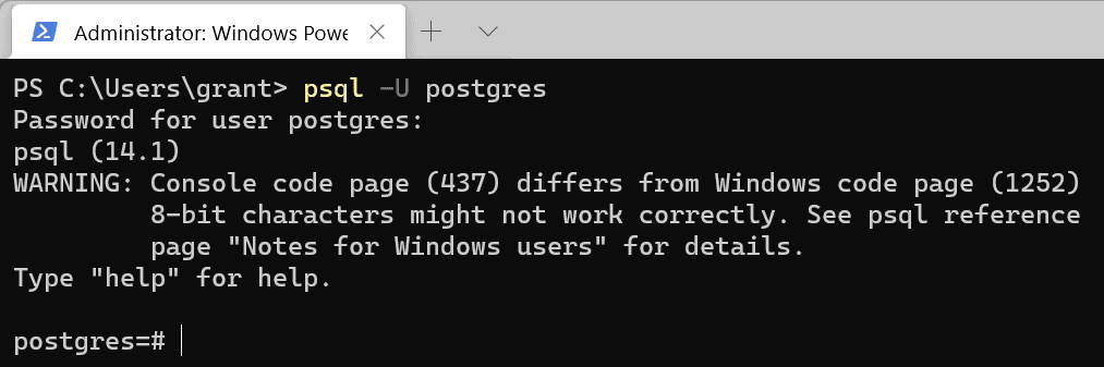
The command starts a psql session, and the user name I wish to log in with is ‘postgres’, the default user. This command assumes I’m running locally through either a container or a service using localhost and the default port. If any of that is not valid, you’ll have to change settings. Hitting enter will bring you to a password prompt. Use the password you used in whichever system you set up above, and you’ll end up at a prompt:

An image showing how to connect to PostgreSQL with psql

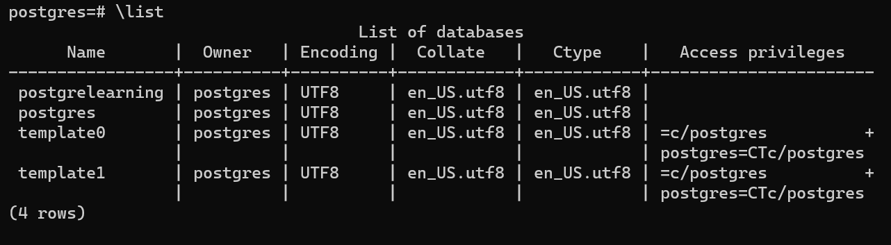
There are many commands you can run within psql. For example, to see the databases use the command:

\list

The output will look something like this:

List of databases from PosgreSQL using the \List command

You can then connect to one of those databases like this:

\connect postgrelearning

You’ll then see the prompt has changed to show the different database you’re in:

Image showing how to connect to the postgrelearning database

From there, you’re using SQL within PostgreSQL. Just remember that you must use the semicolon as a statement terminator to make the query run.

pgAdmin

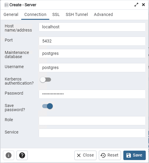
Another tool you can use is pgAdmin, a browser-based tool for working with your PostgreSQL databases. Like with so much else these days, you can download an executable and install it or grab a container. You’ll have to create an account with a password to use this tool. Connecting is the same as anything else; put in the name or the IP address, port, login, and password.

Image showing the pgAdmin tool connection properties

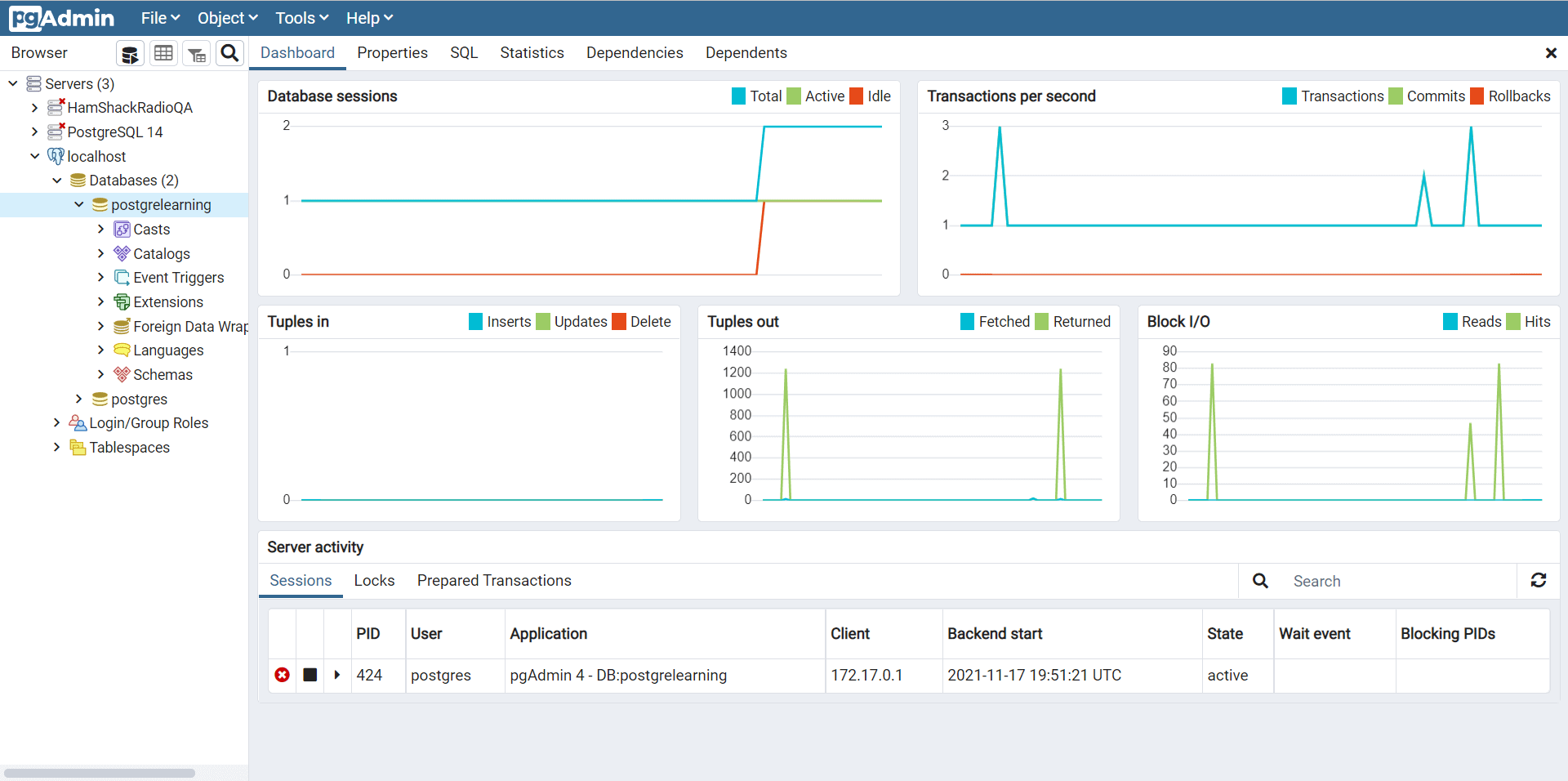
After connecting, you get something that looks like this:

Image showing the pgAdmin tool dashboard and servers

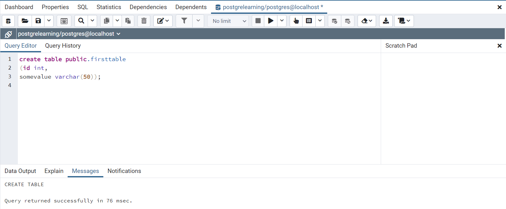
You get some monitoring and other functionality for administering the server and databases. You also get a full query editor:

Image showing the query editor in pgAdmin and a create table statement

You get formatting and some limited code completion. There’s the ability to look at explain plans.

pgAdmin 4 is up to version 6.1. Yeah, I find that confusing too, but that’s what’s going on. It’s a pretty darned complete management tool, even if it’s browser-based.

Azure Data Studio

Azure Data Studio is a multi-platform query tool that currently works with Microsoft SQL Server and PostgreSQL. It’s primarily a development tool for writing queries, although an object explorer lets you look through objects within the database.

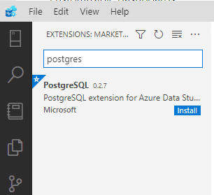
To connect to PostgreSQL, you’ll have to install the PostgreSQL extension to Azure Data Studio.

Image showing how to add the PostgreSQL extension for Azure Data Studio

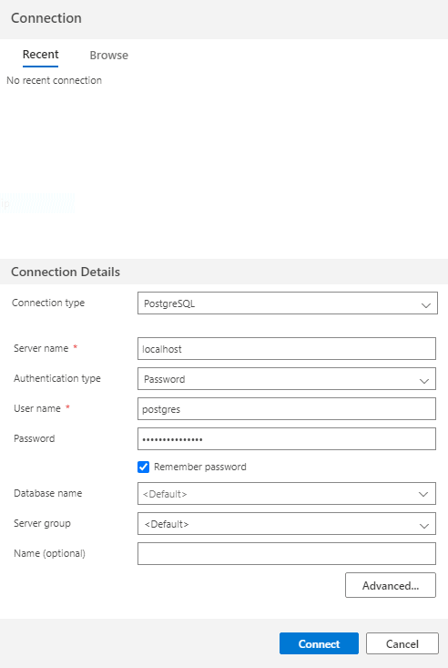
Connections are the same as with the other tools. Fill in the server name or IP, the port if different from the default, user name, and password.

The connection dialog to connect to PosgreSQL from Azure Data Studio

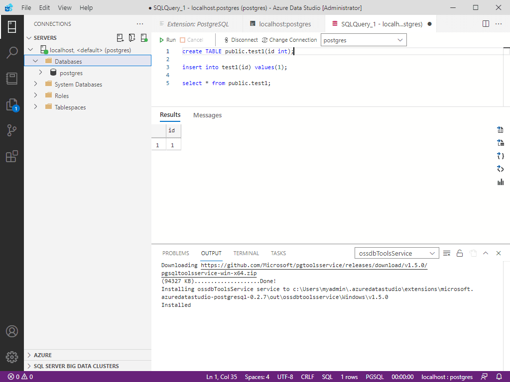
The query editor has good code completion. Running queries looks like this:

Image showing servers on the left and the query editor with code to create a table, populate it with one row and then select. All in Azure Data Studio

Conclusion

I’ve no doubt I’m making some mistakes as I learn this stuff, and I’ll include updates as we go along. This article covered enough to get anyone started within PostgreSQL. From a service, to a container, to a web service, you can run PostgreSQL. Once it’s running, you have multiple tools that can easily connect up to your server or databases. From there, it’s just a question of learning. I’m going to start on the one action I would look to if I were taking on this stuff for a job, backups.


The post Connecting to PostgreSQL: Learning PostgreSQL with Grant appeared first on Simple Talk.


from Simple Talk https://ift.tt/3CI025X
via

Monday, November 22, 2021

Dynamic Data Mask is now useful and no one noticed it

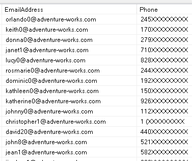
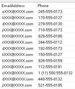
Dynamic data mask is a very interesting security feature allowing us to mask critical fields such as e-mail, phone number, credit card and so on. We can decide what users will be able to see the value of these features or not.

This feature faced many flaws when it was released, but I believe it’s stable now, although It’s not the main security feature you should care about, it can still be very useful.

However, until very recently, this feature was not very useful. If you mask many fields in many different tables, the fields may require different permission levels in order to be unmasked.

The only permission control provided for Mask and Unmask fields where this: See everything masked or everything unmasked. In this way, the feature was not useful, because there is not doubt that phone number and credit card should have different permission levels.

Finally, the granular permission control for Data Mask is available in Azure SQL Databases. The feature became way more useful and with so many news around these weeks, not many people noticed.

Test Environment

Let’s test this feature using the AdventureWorksLT. We can provision this database in Azure SQL by choosing to provision a sample database.

Applying the Data Mask

alter table SalesLT.Customer
     alter column EmailAddress nvarchar(50)
        masked with (function=’email()’)
go
alter table SalesLT.Customer
      alter column Phone nvarchar(25)
        masked with(function=‘partial(3,”XXXXXXXXX”,0)’)
go

Create Roles to control Mask Permissions

Control permissions in a field level is something complex. A good practice to do this is using database roles. Let’s create database roles for this and set the permission of these roles as data reader to make the example easier.

Create Role EmailView
go
Create Role PhoneView
go
Alter Role db_datareader add member EmailView
go
Alter Role db_datareader add member PhoneView
go

Grant the unmask peremission

On our example, we will grant the unmask permission over each field for the different database roles. The statements will be like this:

Grant UnMask on SalesLT.Customer(Phone) to PhoneView
go
Grant UnMask on SalesLT.Customer(EmailAddress) to Emailview
go

The granular unmask permission also would allow to grant permission schema level:

Grant UnMask on Schema::SalesLT to CustomRole

Or also on table level:

Grant UnMask on SalesLT.Customer to CustomRole

Anyway, now making the data mask feature really useful.

Create user CanReadEmail with password=‘9646xpahmW’
go
 
Create user CanReadPhone with password=‘9646xpahmW’
go
alter role EmailView add member CanReadEmail
go
alter role PhoneView add member CanReadPhone
go
 

Test the users and UnMask Feature

Execute as user=‘CanReadEmail’
 
select * from SalesLT.Customer
 
revert

This first user can read the phone, but not the e-mail:


Execute as user=‘CanReadPhone’
 
select * from SalesLT.Customer
 
revert

This 2nd user can read the e-mail but not the phone:


Conclusion

We have a new powerful security feature on our hands to work with and I hope this feature to be in SQL Server 2022 as well

The post Dynamic Data Mask is now useful and no one noticed it appeared first on Simple Talk.


from Simple Talk https://ift.tt/3CAB0Ws
via

Wednesday, November 17, 2021

Mighty Tester – Miracle worker

Image showing a 6 panel strip. Manager ask for a big project that must be perfect and with lots of testing. Then asked that it be done in an hour.

The post Mighty Tester – Miracle worker appeared first on Simple Talk.


from Simple Talk https://ift.tt/3CpAvhK
via

10 reasons why Python is better than C# (or almost any other programming language)

Nearly 10 years ago, I wrote an article on this website comparing C# unfavourably with Visual Basic, which prompted many comments, roughly equally divided between praise and censure. My favourite two (now sadly removed) were “Your website looks like Teletubbieland” (which had some truth at the time, but wasn’t strictly relevant) and “You know f*** all about C#”, which had relevance but – I believe – less truth (and in its original form didn’t have any asterisks either!). To celebrate this anniversary, I’ve decided to reawaken all of you slumbering C# trolls with 10 reasons why Python is better than C# (and better than most other programming languages, too, it has to be said).

1 – Indented code blocks

These are just beautiful! Here’s how you can write a loop and condition in Python to play Fizz-Buzz in Python:

for integer in range(1,11):
    # for first 10 numbers
    if integer % 3 == 0:
        print(integer, "Fizz")
    elif integer % 5 == 0:
        print(integer,"Buzz")

Notice anything? There are no silly { } brackets to denote when a condition or loop block starts and ends because Python can infer this from the indentation. Why type characters when you don’t have to?

2 – Self-declaring Variables

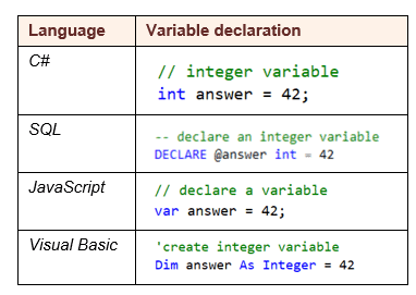
Here’s how you can declare variables in four programming languages:

An image showing how to declare variables in several languages

In Python, you don’t – and can’t – declare variables. Instead, you just assign values to them:

# create a variable to hold the meaning of life
meaning_of_life = 42

Python then creates a variable of the appropriate type (you can prove this by printing out its value):

# show the type of this, and its value
print(type(meaning_of_life),meaning_of_life)

This code would show <class ‘int’> 42. Another nice thing about Python variables is how simple the data types are: there are only integers, floating point numbers, strings, and Boolean values, which is pretty much all a programming language needs, dates being just formatted numbers when all’s said and done).

Now C# programmers will – like I did – initially throw their arms up in horror at this, but haven’t we all been writing lines of code like this for years?

// store life's meaning
var meaningOfLife = 42;

This statement does exactly the same thing: it sets the type of the variable from the context.

I’ve found not having to declare the type of variables strangely liberating, to the extent that I now resent having to declare variables when I go back to writing code in C# or SQL.

3 – Those modules …

Python is Python because of its modules: literally thousands of add-ins, covering everything from scraping websites to advanced AI tasks.

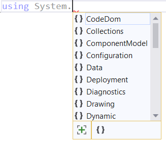
But wait a bit, you may say – C# (at least as it’s written in .NET, which is surely the most common implementation) has “modules” too. Here are just a few of the ones in the System namespace:

An image showing a Using statement in C# and all the options

The answer to which is: yes, it does, but … Python modules are so much easier to use. To illustrate this, let’s take an example: looping over the subfolders in a folder. Here’s how you could do this in Python:

import os
# get a list of all the files in a folder
files = os.listdir(r"C:\__work\\")
# loop over these files
for file in files:
    # show its name
    print(file)

Here’s the approximate equivalent C# code:

using System.IO;
var folder = new DirectoryInfo(@"C:\__work\");
foreach (DirectoryInfo dir in folder.GetDirectories())
{
Debug.WriteLine(dir.Name);
}

I’m aware that it’s subjective, but I find the Python modules to be almost without exception more logically constructed and easier to learn than the equivalent .NET ones, for example.

4 – Simplicity of Data Structures

C# has (deep breath now) the following data structures: Array, ArrayList, Collection, List, Hashtable, Dictionary, SortedDictionary, SortedList. These implement the IEnumerable or IDictionary interfaces. If you’re thinking of learning C#, I’ve probably just put you off for life!

Python has four structures: lists, tuples, dictionaries, and sets, although the first two are virtually identical from the programming point of view. Purists will say that you need all the different data types that C# provides, but trust me, you don’t.

It’s not just that Python only has a few data structures; the ones it does have are so easy to use. Here’s how you create a sorted list of fruit, for example:

# create an empty list
fruit = []
# add some fruit
fruit.append("Pears")
fruit.append("Apples")
fruit.append("Bananas")
# sort this
fruit.sort()
# print

print(fruit)

Programming doesn’t get any more straightforward than this!

5 – Slicing

I’m not generally a fan of languages that try to cram as much logic into as few characters as possible (that’s why I don’t like regular expressions and didn’t get on with Perl).

However, slicing sequences has the big advantage that it’s used everywhere in Python, so once you’ve learnt a few simple rules, you can pick out anything you want. And there’s a certain beauty in code like this:

# the seven deadly sins
sins = ["pride", "envy", "gluttony", "greed", "lust", "sloth", "wrath"]
# every other one, but missing the first and last
# ie ['envy', 'greed', 'sloth']
selected_sins = sins[1:-1:2]
print(selected_sins)

The great thing about slicing is that it carries through to everything. Once you’ve learnt how to slice a tuple, for example, you’ve also learnt how to slice a multi-dimensional array (in numpy) or an Excel-style dataframe (in pandas) or any other sequence of items.

6 – For loops

C# has two separate loop structures, depending on whether you’re looping over numbers or objects, as shown by these two examples:

// first 5 numbers
for (int i=0; i <= 5; i++) {
Debug.Print(i.ToString());
}
// words in a string
string[] words = {"Simple","Talk"};
foreach (string word in words)
{
Debug.Print(word);
}

Here is the same code in Python:

# first 5 numbers
for i in range(1,6):
    print(i)
# words in a string
words = {"Simple","Talk"}
for word in words:
    print(word)

Notice that not only is the Python for loop syntax simple and easier to understand, but there’s only one version of it (unlike in C#, where sometimes you use for and sometimes foreach).

7 – List comprehensions

A list comprehension is one of the most beautiful programming constructs I’ve seen. You can use it as a substitute for C# lambda or anonymous functions, and the result is transparent.

Here’s an example listing out the cubes of all the even numbers up to 10:

# cubes of even numbers up to and including 10
# (would give [8, 64, 216, 512, 1000] as output)
print([n ** 3 for n in range(1,11) if n % 2 == 0])

You could of course do this the long way round:

for n in range(1,11):
    if n % 2 == 0:
        print(n ** 3)

It’s hard to think how you could improve the syntax of the first method: show me this for these numbers where this condition is true.

8 – Sets

I said just now that list comprehensions are beautiful, but so too are sets.

For example, the way to remove duplicates from a list of items in Python is just to convert the list to a set (since sets can’t contain duplicate items, any duplicates will be removed), then convert the set back to a list. Like this, say:

# this contains some duplicates
languages = ["C#","Python","VB","Java","C#","Java","C#"]
# this set can't
language_set = set(languages)
# convert back to a list
languages = list(language_set)
# this will give: ['C#', 'Java', 'Python', 'VB']
print(languages)

However, sets don’t just provide an elegant way to remove duplicates from lists; they also allow you to find the intersection or union of two groups of items (those long-ago maths lessons learning Venn diagrams weren’t wasted after all!).

Pretty much everything you need to know about sets in Python is covered by these few lines of code:

# create two sets: Friends characters and large Antarctic ice shelves
friends = {"Rachel","Phoebe","Chandler", "Joey","Monica","Ross"}
ice_shelves = {"Ronnie-Filchner", "Ross", "McMurdo"}
# show the intersection (elements in both lists)
print(friends & ice_shelves)
# show the union (elements in either list)
print(friends | ice_shelves)
# show the friends who aren't ice shelves
print(friends - ice_shelves)
# elements in either set but not both
print(friends ^ ice_shelves)

This code would give this output ( “Ross” is the only item in both lists, for example):

An images showing the output of sets in Python

9 – Working with files and folders

Virtually everything to do with files and folders is easier than you think it’s going to be. Want to write out the contents of a list? No need to import modules – just do this :

# list of 3 people
people = ["Shadrach","Meshach","Abednego"]
# write them to a file
with open(r"c:\\wiseowl\people.txt","w") as people_file:
    people_file.writelines("\n".join(people))

Want to export this as a CSV file? Just use the built-in csv module:

import csv
# write student amesto a file
with open(r"c:\\wiseowl\students.csv","w",newline="") as people_file:
    potter_file = csv.writer(people_file)
    # use this to write out 3 rows
    potter_file.writerow(["Harry", "Gryffindor"])
    potter_file.writerow(["Draco", "Slytherin"])
    potter_file.writerow(["Hermione", "Gryffindor"])

I could go on to show reading from or writing to JSON files, Excel files, any files using pandas … Python modules make coding as easy as it can be!

10 – The quality of online help

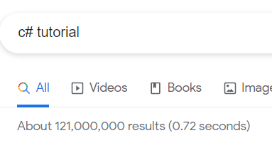
Here are the results of a search using a well-known search engine (!) for the phrase C# tutorial:

An images showing the number of results when searching on C# tutorial

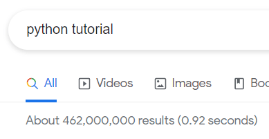
Here are the results for the same search using the phrase Python tutorial:

An image showing the results of searching on Python tutorial

But it’s not just that Python has nearly four times as many tutorial page results: the tutorials themselves are much better, IMHO.

Two reasons not to like Python

It would be disingenuous to end this article without giving two areas in which Python doesn’t compare well with other languages like C#.

The first way in which Python underperforms is that it’s so hard to get started. In C#, you’re probably going to choose Visual Studio as your development environment, and while you will have teething problems, at least everything is integrated. In Python, you have to choose whether to use Visual Studio Code, PyCharm, Jupyter Notebook, or any of a dozen other candidates for your IDE (Integrated Development Environment). Even when you’ve chosen your IDE, you’ll still have to learn how to set up “virtual environments” in which you can install modules for different applications that you’re creating so that they don’t interfere with each other. None of this is straightforward, and it’s a serious impediment to getting started with Python.

The second way in which Python underperforms is that it isn’t always strongly typed. This limitation is best illustrated by an example. Consider this segment of Python code:

def add_numbers(first:int,second:int) -> int:
    # add the two numbers together
    return first + second
# test this out
print(add_numbers(3,5))
# now test this with some text
print(add_numbers("Simple","Talk"))

It creates a function to add two numbers together, then calls it twice. The first call will give 8 (the sum of 3 and 5), while the second will give “SimpleTalk” (treating the “+” in the function as a concatenation symbol).

The problem is this line:

def add_numbers(first:int,second:int) -> int:

This is sometimes referred to as duck typing: if it looks like a duck and quacks like a duck, it’s probably a duck. Except that this looks like an integer and is passed as an integer – and yet is happily accepting a string into the function. The data types are just hints, it turns out: a serious limitation.

Interpreted not compiled

One other big difference between Python and other languages is that the former is interpreted rather than compiled. What this means is that when you run a Python program, the instructions are read as text in sequential order (no executable file is constructed first from the human-readable statements translated into machine-readable language). However, I still can’t decide if this is a good or bad thing, so I have left it off both lists above!

Why Python is better than C#

Python was created by Dutch programmer Guido van Rossum to be as easy to use as possible; he succeeded in his aim! Although the Monty Python references in documentation get a bit tedious (even for this diehard fan), if you’re an experienced C# programmer, you will enjoy the simplicity of programming in Python.


If you like this article, you might also like 10 Reasons Why Visual Basic is Better Than C#


The post 10 reasons why Python is better than C# (or almost any other programming language) appeared first on Simple Talk.


from Simple Talk https://ift.tt/3Fq3XpF
via

Tuesday, November 16, 2021

Introduction to DAX for paginated reports

SQL Server Reporting Services (SSRS) may have been around for nearly 20 years, but it simply refuses to go away. Its latest lease of life is evidenced in the release of the Paginated Report visual for Power BI that allows developers to include paginated reports inside Power BI dashboards. In many ways, this is a natural extension of the existing ability of the Power BI Premium Service to load and display paginated reports – and of course, the well-established use of SSRS as the reporting tool of choice to visualise information held in tabular SQL Server Analysis Services data warehouses.

However, if you are a traditional SSRS report developer, who is in the habit of using SQL as the query language for your reports, then using DAX to query source data can be initially disconcerting. Equally, the DAX that you use to extract data for reports can be very different from the DAX that you may be used to writing when creating Power BI dashboards (or even extending Excel Pivot tables).

The aim of this article – and the three that follow – is to help you overcome any initial challenges when sourcing data for paginated reports from a Power BI dataset. This includes a series of suggestions to make your life easier when delivering paginated reports – whether as a separate report or as a visual inside a Power BI dashboard with Power BI Premium (which includes Premium per user).

What I am not attempting to do is to provide either an introduction to paginated report development or to DAX. I am presuming that you have a grasp of the fundamentals of each of these and that your objective is to adapt your existing knowledge to use DAX as the source of data for paginated reports. This means that I will not explain how to create Power BI dashboards, load datasets into the Power BI Service, create dataflows, or write DAX measures – or indeed any of the “classic” Power BI techniques.

Within the scope of these objectives, it is time to move on to an initial overview of how to create paginated reports using DAX.

The paginated report developer’s toolkit

Creating and perfecting paginated reports for Power BI requires a very simple set of tools. The good news is that all of them are completely free. The bad news is that paginated reports are only available in a Premium or Premium per user workspace.

The core tool used to create the paginated reports that you will subsequently upload to the Power BI Service is Power BI Report Builder. I suggest this as the report development tool simply because:

  • It is free, quick to install, and has no licensing hassles
  • It connects automatically to Power BI datasets in the Power BI Service

To write and debug DAX, I strongly advise that you download and install the brilliant and irreplaceable DAX Studio.

Finally, an advanced text editor such as Notepad++ is invaluable for some of the more advanced tweaking of the .Rdl files that you create using Power BI Report Builder.

Sample data

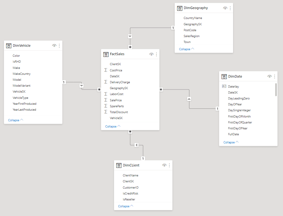
To allow you to concentrate on DAX, and not waste time setting up a complex environment, the accompanying sample data for these articles is a single Power BI Desktop file. This file (CarsDataWarehouse.pbix) contains one fact table and four dimensions. You can see the star schema of the data in the following image:

This dataset is deliberately lightweight and contains only a few hundred records to ensure that you spend as little time as possible waiting on query execution when you run your own DAX queries.

Power BI Dashboard and report integration

If you wish to follow the examples in these articles, you will need to imitate a real-world Power BI environment. I will presume that you have access to a Power BI Premium environment and have the rights to upload both .Pbix and .Rdl files. The unfortunate limitation at present is that you cannot perfect your paginated report integration skills if all you have is a free Power BI account. To get started, upload the CarsDataWarehouse.pbix file to Power BI Service.

Building paginated reports using Power BI datasets

To ensure that the prerequisites are in place, here is how you can connect to an existing Power BI dataset in the Power BI Service from Power BI Report Builder. This dataset can be as simple as a version of the sample dashboard CarsDataWarehouse.Pbix that you have previously uploaded.

  1. Open Power BI Report Builder.
  2. Create a Blank Report
  3. Right-click Data Sources and select Add Power BI Dataset connection.
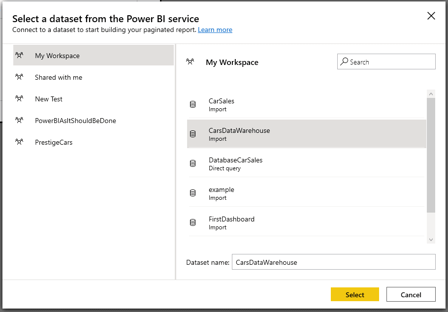
  4. Select the dataset in the dialog as shown below and click Select.

You can now build SSRS reports that will use the data in the Power BI Service using DAX as the query language.

Automated query writing

If the data you need is extremely simple (a list without parameters and no filtering), then you can have Power BI Report Builder write the DAX for you, like this:

  1. Right-click on Datasets and click Add Dataset.
  2. Select the CarsDataWarehouse data source.
  3. In the Dataset Properties dialog, click on the Query Designer button.
  4. Drag the Attributes and measures you wish to include in the report dataset into the lower right-hand pane.
  5. Test the query by clicking Click to execute the query.
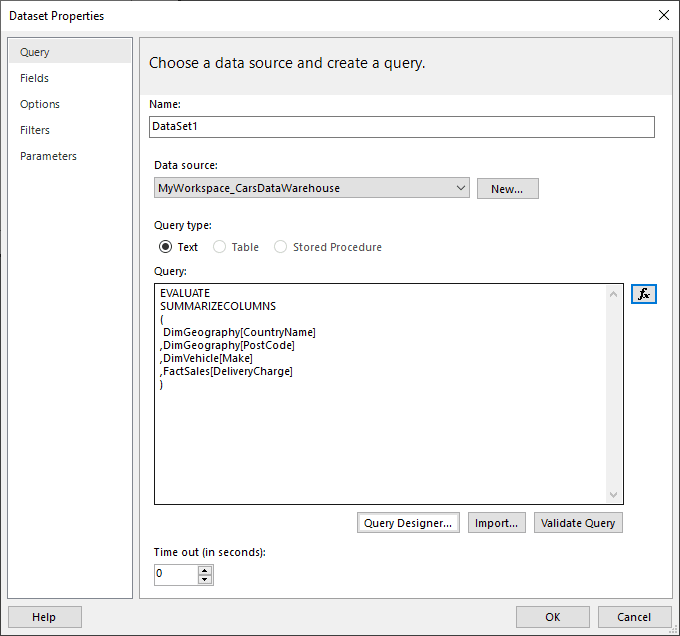
  6. Click OK. You will see the resulting, automatically-generated DAX query in the Query area as shown below:

  1. Click OK to create the dataset.

As you can see, this is very simple and very easy. However, I would never suggest that you build any but the simplest of output datasets in this way. The reasons for avoiding this approach are:

  • It only works for simple lists.
  • It creates excessively complex DAX that is hard to understand and modify when you add parameters and filters.
  • It has an annoying tendency to crash for complex queries
  • Using the Query Designer automatically overwrites any existing query – even carefully hand-crafted DAX queries – which rapidly becomes extremely frustrating.

Consequently, I advise avoiding the query designer as far as possible and using DAX Studio to write – and perfect – the DAX that you use to drive your paginated reports.

Uploading paginated reports to the Power BI Service

One of the advantages of using Power BI Report Builder to create .RDL files, is that it imitates Power BI Desktop in that it can connect to the Power BI Service and update the current file in a couple of clicks. Simply click the Publish button in the Home menu and choose the destination workspace for the current paginated report file. Of course, you will have to log in to the Power BI Premium service (just as you would when developing dashboards using Power BI Desktop) first.

Alternatively, you can log in to Power BI and upload an .Rdl file to the Power BI Service just as you would upload a .pbix file.

Alternatives to the Query Designer

If the Query Designer inside Power BI Report Builder is best avoided, what is the alternative? Quite simply, the most efficient alternative that I can suggest is:

  1. Build and test DAX queries using DAX Studio.
  2. Copy the query into Power BI Report Builder like this:
    1. Right-click on Datasets and click Add Dataset.
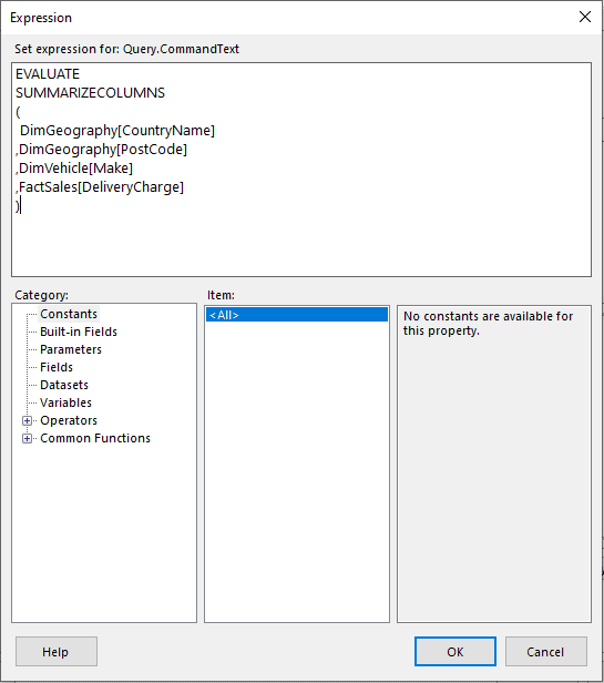
    2. Click on the Expression Editor (Fx) button to the right of the Query area.
    3. Paste the DAX query (from DAX Studio) into the Expression Editor, as shown in the following figure:

  1. Click OK twice.

This approach has multiple advantages. Amongst the main ones are:

  • You can build, test and debug DAX in an IDE designed specifically for DAX development – including searching for attributes in the dataset and drag and drop, search and replace, etc.
  • DAX Studio provides comprehensible error messages if anything does not work quite as expected.
  • Coding errors are less likely which is particularly important as many DAX errors cause the Power BI Report Builder either to hang or to crash.
  • You can preview the output data.
  • You can develop complex DAX that is simply not practical to write in the notepad-style editor of Power BI Report Builder.

SSRS parameters in DAX

Of course, you are inevitably going to need to filter the data when it comes to returning data from a Power BI dataset to a paginated report. SSRS has handled user parameters from its outset as a data filtering technique and can, of course, handle parameter passing to DAX-based Power BI data sources.

Creating DAX-driven parameters

The first thing to do is to populate SSRS parameters from the underlying dataset using DAX. The basic principles concerning populating DAX parameters are very similar to those that you may be used to applying when using SSRS with SQL or MDX as the query languages:

  • Create one DataSet in the paginated report for each SSRS parameter that you need to populate.
  • Create another separate dataset if you are pre-selecting multiple default items from a parameter list automatically.

Populating the parameter list

The DAX that you use to query a Power BI dataset to return a list of parameter elements is straightforward. It is nearly always something like the following:

EVALUATE
SUMMARIZECOLUMNS
(
DimGeography[CountryName]
)

It is worth noting that:

  • You do not need to specify a distinct list as SUMMARIZECOLUMNS() does this for you automatically.
  • Remember that the parameter values are case-sensitive if you enter one or more values manually in the list of default values. You then use this dataset as the source for the available values in the parameter list by selecting Get values from a query as the Available Values setting in the parameter properties.

Date-based parameters

If you are setting a start date (for instance) as the default value for a parameter, the minimum date value from a field in a dataset can be calculated using a DAX query that applied the FIRSTDATE() function like this:

EVALUATE FIRSTDATE(VALUES(DimDate[DateKey]))

Conversely, that last date in a field can be queried using the LASTDATE() function – something like this

EVALUATE LASTDATE(VALUES(DimDate[DateKey]))

Applying parameters in paginated reports

Once you have created one or more parameters in a paginated report, you will, of course, need to apply them to the DAX that you are creating to return data to the report. As you just saw, external parameters in DAX are simply variables that start with the @ sign. As you might expect, the art is to apply these variables inside the filters so that the resulting data conforms to your requirements.

Simple parameter passing

To start at the beginning, let’s take a (very) simple output using a single filter that does not yet use a parameter – like this:

EVALUATE
SUMMARIZECOLUMNS(
 DimCLient[ClientName]
,DimVehicle[Make]
,DimVehicle[Model]
,FILTER(VALUES(DimVehicle[Color]), DimVehicle[Color] = "Red")
,"Sales", SUM(FactSales[SalePrice])
)

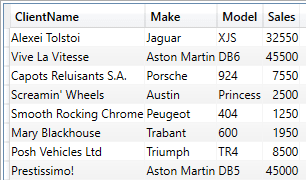
The shortened output from this short piece of DAX is:

Assuming that you have created an SSRS parameter that contains a list of colours, and that the name of this parameter is @Colour, the previous DAX snippet, tweaked to enable parameter passing into the DAX, becomes:

EVALUATE
SUMMARIZECOLUMNS(
 DimCLient[ClientName]
,DimVehicle[Make]
,DimVehicle[Model]
,FILTER(VALUES(DimVehicle[Color]), DimVehicle[Color] = @Colour)
,"Sales", SUM(FactSales[SalePrice])
)

This also introduces the use of external parameters in DAX. As you can see, they are extremely simple. An external parameter:

  • Starts with @
  • Does not contain spaces

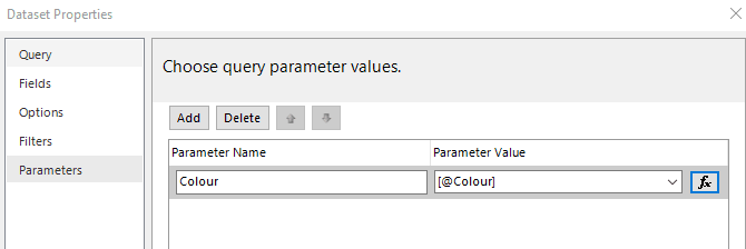
When creating a dataset filtered by a parameter, you must create the query first without the filter. Link the parameter in the Parameters tab and then add the filter. You’ll get an error message if you try to add the filter before the parameter is linked.

Graphical user interface, text, application, email Description automatically generated

Notes:

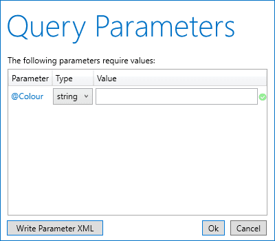
As previously mentioned, DAX Studio allows you to test this approach by entering parameters when you run the DAX. Running the above DAX will display the following dialog:

A single parameter can be reused at multiple places inside the DAX.

  • Date parameters require that you enclose the date parameter in the VALUES() function – like this (for a parameter named @EndDate):
,FILTER(VALUES(DimDate[DateKey]), DimDate[DateKey] >= VALUE("12/29/2020 12:00:00 AM") && DimDate[DateKey]<= VALUE(@EndDate))

It is worth noting that, given the fragility of Power BI Report Builder, you have to add, update or remove any SSRS parameters that you are using in a report dataset before modifying the query – or, alternatively, modify the query in Notepad++ then add the parameters in Power BI Report Builder. In any case, the input parameters must be aligned to the parameters used in the DAX or Power BI Report Builder will probably hang until you close it and start over. It is also worth remembering that any parameters that you define must be used in the DAX. In contrast, merely adding a parameter to a report and not using it in the dataset will not produce any negative effects.

Populate parameters with all elements selected

The DAX needed if you want to define an SSRS dataset that sets all the elements in a multi-select parameter list as default values are slightly out of the ordinary. You need to add the KEEPFILTERS() function to the DAX, like this:

EVALUATE
SUMMARIZECOLUMNS
(
DimGeography[CountryName]
,KEEPFILTERS(FILTER(ALL(DimGeography[CountryName])
             ,NOT ISBLANK((DimGeography[CountryName]))))
)

You then use this dataset as the source for the default values in the parameter list by selecting Get values from a query as the Available Values setting in the parameter properties.

Please note that the effect of this definition of default values does not currently display correctly in preview in Power BI Report Builder. To see it work as you expect it to, you have to load the report into the Power BI Service and run the report from there.

Be warned, however, that a multi-value parameter needs careful handling inside the DAX itself. You need to look ahead to the next but one section RSCustomDaxFilter actually to use the multiple elements that you have selected.

Parameterized parameters

Very much as you do for SQL sources, you can create cascading parameters where one parameter’s output becomes an input parameter for a second parameter. This allows you to imitate the hierarchical slicers in Power BI dashboards.

For example, assuming that a parameter named Make exists, and that you want the selected make to filter the items displayed in a Model parameter, you can use the following DAX to return the list of available elements in the Model parameter:

EVALUATE
SUMMARIZECOLUMNS(
DimVehicle[Model]
,FILTER(VALUES(DimVehicle[Make]), DimVehicle[Make] = @Make)
)

Of course, this requires a couple of basic structural elements:

  • The Make parameter is moved above the Model parameter in the Parameters list in Power BI Report Developer.
  • You define Make as an input parameter for the Model dataset you create using the code snippet above.
  • The Model parameter can then be used to filter the main report

RSCustomDaxFilter

Handling multi-select parameters is one aspect of parameter passing from SSRS to DAX that was tricky initially (but that has fortunately been solved for a while now).

The currently recommended approach is to use the SSRS function RSCustomDaxFilter() to handle multiple selections in the SSRS report interface. This function is not standard DAX (it is not recognised by DAX Studio, for instance) and only works in the DAX used in .Rdl files.

This function required four elements. They are:

  1. Parameter Name
  2. Comparison/Condition
  3. Field to use
  4. Data Type

The RSCustomDaxFilter() function is probably best explained using a simple example. Take a look at the following piece of DAX:

EVALUATE
SUMMARIZECOLUMNS(
 DimCLient[ClientName]
,DimVehicle[Make]
,DimVehicle[Model]
,RSCustomDaxFilter(@Colour, EqualToCondition, [DimVehicle].[Color], String)
,"Sales", SUM(FactSales[SalePrice])
)

This filter takes multiple selected elements passed from the Colour parameter popup list in a paginated report and applies them as an OR filter to the underlying DAX.

Let’s take a closer look at the four elements of the function:

  1. ParameterName – (@Colour in this example). This is simple as it is the name of the input parameter as defined in the Parameters pane of the Dataset properties.
  2. Comparison/Condition – (EqualToCondition in this example). This is the equality operator (=).
  3. Field to use– ([DimVehicle].[Color]in this example). This refers to the dataset field that must be used to filter data.
  4. Data Type– (String in this example) This specifies the datatype of the parameter.

Notes:

You cannot write the field name inside the RSCustomDaxFilter() function as CaseProduct[Key Ingredients] or ‘CaseProduct’[Key Ingredients] (as you would in normal DAX). You must wrap both the table and the field names in square brackets and separate them with a period. I suspect that this is a possible hangover from the MDX-style approach used in SSRS when handling non-SQL data sources.

The possible datatypes that you can use are:

  • Int64
  • String
  • Double
  • DateTime
  • Boolean
  • Currency

The possible conditions that you can use are:

  • EqualToCondition
  • Not EqualToCondition

To make things clearer, the following is a valid application of RSCustomDaxFilter():

RSCustomDaxFilter(@SalesAmount,NotEqualToCondition,[FactSales].[SalePrice],Double)

In practice, you can use RSCustomDaxFilter() where you would otherwise use FILTER() inside the SUMMARIZECOLUMNS() function when you need to accept multiple alternative parameter inputs to filter data. You can, of course, mix the two approaches as well as using use the complete range of possibilities of SUMMARIZECOLUMNS() as the following example shows:

EVALUATE
SUMMARIZECOLUMNS(
 DimCLient[ClientName]
,DimVehicle[Make]
,DimVehicle[Model]
,FILTER(
        VALUES(DimDate[DateKey])
        ,AND(DimDate[DateKey] >= VALUE("01/01/2020")
        ,DimDate[DateKey]<= VALUE("12/30/2022"))
        )
,FILTER(VALUES(DimVehicle[Color]), DimVehicle[Color] = @Colour)
,RSCustomDaxFilter(@SalesAmount
                   ,EqualToCondition
                   ,[FactSales].[SalePrice]
                   ,Double)
,"Sales", SUM(FactSales[SalePrice])
)

Unfortunately RSCustomDaxFilter() is not recognised by DAX Studio. However, there are workarounds that I will give in the final article in this series. Even more unfortunate is that adding RSCustomDaxFilter using Power BI Report Builder can also cause intermittent issues. So you are probably best advised to add this particular filtering approach to the DAX for the .Rdl file using Notepad++.

Some useful tips

I want to conclude this introductory article with a couple of practical tips that should help when starting out using DAX to query datasets for SSRS reports.

The SAMPLE() Function

Power BI datasets can become extremely large. The corollary is, inevitably, that running sample queries on industrial-sized data sources can take up valuable development time.

One solution to ease the pain – and make queries run considerably faster when carrying out initial development – is the judicious application of the SAMPLE() function. For instance, you can simply wrap a DAX query in SAMPLE() as follows:

EVALUATE
SAMPLE
(
10
,SUMMARIZECOLUMNS
(
DimGeography[CountryName]
,DimCLient[ClientName]
,"Total Sales", SUM(FactSales[SalePrice])
)
,DimCLient[ClientName]
)

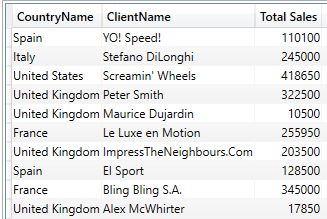
The SAMPLE() function merely requires a number as the first element (the number of sample records that you want the query to return) and the DAX query as the second element. Of course, you have to remember to remove SAMPLE (and the final right parenthesis) once development is complete to allow accurate unit testing. The entire output from this piece of DAX is:

Dummy measure

If you are returning wide lists, that means DAX queries that contain many fields from different tables (whether or not the data is filtered) using SUMMARIZECOLUMNS(). You can easily find yourself facing long query times or even timeouts. The simple solution to resolve this challenge is to add a calculated value (directly calculated or using an existing measure) at the end of the SUMMARIZECOLUMNS() function – even if you will not need to display the calculation output in the actual report.

You can see this technique applied in the following code sample:

EVALUATE
SUMMARIZECOLUMNS
(
 DimVehicle[Make]
,DimVehicle[Model]
,DimGeography[CountryName]
,DimGeography[SalesRegion]
,DimGeography[Town]
,DimCLient[IsCreditRisk]
,DimCLient[IsReseller]
,DimCLient[ClientName]
,DimVehicle[MakeCountry]
,DimVehicle[VehicleType]
,DimVehicle[IsRHD]
,DimVehicle[ModelVariant]
,"DummyMeasure", COUNT(FactSales[SalePrice])
)

The output from this piece of DAX adds an extra column. However, the increase in the processing speed more than compensates for any increase in data size – and you do not have to use the Dummy column in your paginated report.

It is worth noting that the data output slowdown does not seem to occur when returning multiple fields from a single table in the underlying dataset.

The future articles in this series contain many more hints and tips that you could find helpful when facing more complex challenges.

Next steps

Armed with what you have read in this article, you should be able to create paginated reports that you can either load directly into the Power BI Service or use when creating Power BI visuals using the Paginated Report visual in Power BI Desktop.

However, there is still a lot to learn when using Power BI datasets and DAX as the basis for paginated reports. The next step is to extend the basic approaches that you saw in this article with more advanced DAX techniques that enable you to filter the source data for the paginated reports that you want to deliver. This is the subject of the next article.


The post Introduction to DAX for paginated reports appeared first on Simple Talk.


from Simple Talk https://ift.tt/3DmDRTZ
via

BETWEEN the two of us

This past August, I was looking at an online SQL tutorial. One of the sessions in it featured the

BETWEEN predicate, which brought back some memories. In the early days of SQL on the ANSI X3H2 Database Standards Committee, we created the BETWEEN predicate. We wanted the SQL language to sound a bit like English and have shorthand terms for common coding situations. Many of our keywords were stolen from other programming languages or deliberately chosen so that they were not likely to be confused with data elements. The original syntax for the between predicate looks like this:

BETWEEN::=
<test_expression> [NOT] BETWEEN
 <begin_expression> AND <end_expression>

The BETWEEN predicate specifies the inclusive range to test the expression values. The range is defined by boundary expressions with the AND keyword BETWEEN them. Naturally, all the expressions in BETWEEN predicate must be the same data type or cast to it, as in the case of any comparison predicate. This predicate Is defined as a shorthand for:

(<test_expression> >= <begin_expression> 
AND <test_expression> <= <end_expression>)

And the negated version of the predicate

<test_expression> NOT BETWEEN <begin_expression> AND <end_expression>

is equal to:

NOT (<test_expression> BETWEEN <begin_expression> AND <end_expression>)

The grammar for SQL is deliberately picked to be LALR(1). If you don’t remember that from your compiler writing classes, don’t feel bad. It means that SQL can have a little more complicated grammar than many programming languages to sprinkle keywords In places a little more like natural English. It’s important to notice that the BETWEEN predicate uses a closed interval, which includes the endpoints of the range. However, the NOT BETWEEN excludes them.

<test_expression> NOT BETWEEN <begin_expression> AND <end_expression>

is equivalent to

(<test_expression> < <begin_expression> 
OR <test_expression> > <end_expression>)

At some point in these early days, one of the committee members proposed changing the syntax and creating what would now be called a “symmetric BETWEEN” as the default definition. This proposal passed because committees love proposals. Only Microsoft implemented this feature in their Access tabletop database. All the other vendors ignored it, and the proposal was rescinded at the next committee meeting.

But proposals with extended features seem to keep coming back to life. The current ANSI/ISO standard syntax is:

<test_expression> [NOT] BETWEEN [SYMMETRIC | ASYMMETRIC] 
<begin_expression> AND <end_expression>

The keyword ASYMMETRIC has the original functionality, and it is optional. The BETWEEN SYMMETRIC syntax is like BETWEEN except that there is no requirement that the argument to the left of the AND be less than or equal to the argument on the right. Well, not entirely: officially, the <begin_expression> is the minimum, and the <end_expression> is the maximum. This transformation converts a SYMMETRIC BETWEEN into a regular old vanilla BETWEEN.

Intervals in the ISO data model

Several ISO standards deal with the concepts of intervals. From a mathematical viewpoint, the kinds of intervals you can have are (1) Closed, (2) Opened, (3) Half open high, and (4) Half open low. A closed interval includes both the endpoints, like the range in the BETWEEN predicate. An open interval excludes both the endpoints of the range, like the NOT BETWEEN predicate. The half open intervals are open on either the high-end or the low end of the interval range.

A half open interval on the high-end is how ISO models time. We talk about “24-hour time” Or “military time,” but the truth is a day is defined as an interval from 00:00:00 up to 23:59:59.999.. at whatever precision can be measured. If you try and put in “24:00:00 Hrs”, DB2 and other databases will automatically convert it to 00:00:00 Hrs of the next day. Think of it as being like converting a person’s height from 5’18” to 6’6” instead. These conventions get even stranger when you look at how different countries and cultures handle times greater than one day. If an event in Japan runs past midnight, they simply add more hours to the event. For example, an event that ran past midnight might be shown as “25:15:00 Hrs.”

The advantage of the half open interval is easy to see in the ISO 8601 standards, which define how temporal data is represented. You are always sure when an event starts, even if you’re not sure when it will end, so you can use a NULL to mark the end of an event that is in process. This NULL can be coalesced to a meaningful value. For example, sometimes it might make sense to use COALESCE(interval_final_timestamp, CURRENT_TIMESTAMP) To figure out the duration of the interval at exactly the moment the query is invoked. Other times, you might want to use COALESCE(interval_final_timestamp, legally_defined_stop_timestamp).

The BETWEEN predicate is not just used for timestamps. It works perfectly well for numeric ranges and text, too. Numeric ranges can be used to throw things into buckets, which looks reasonably obvious until the three parameter values are of different numeric types. Now you have to consider rounding and casting errors. Even worse, if the parameters are character data with different correlations. As a generalization, you really need to make sure that all three parameters are of the same type. In fact, ranges and text data can get so complicated, I’m just going to ignore them. Let’s just look at numeric ranges.

Report cards

A classic example of reducing values into ranges is converting grades from numeric totals or percentages to a letter grade. The usual convention is that a score in the 90s is an “A”, a score in the 80s is a “B”, a score in the 70s is a “C”, a score in the 60s is a “D” and anything below that is an “F”. I’m choosing to ignore plus or minus options on the letters.

The CASE expression in SQL is executed from left to right, and the first WHEN clause that tests TRUE returns the value in its THEN clause. This means that the order in which you write your tests will control how it executes; not all programming languages work this way. In effect, we have hard-coded half open intervals.

CASE
WHEN score >= 90.000 THEN ‘A’
WHEN score >= 80.000 THEN ‘B’
WHEN score >= 70.000 THEN ‘C’
WHEN score >= 60.000 THEN ‘D’
ELSE ‘F’ END

It is important to notice that this expression will handle somebody who has more than 100 points to qualify as an “A” student. In this example, that’s probably what was intended for extra credit, but this might indicate an error in the data in other schemes. Likewise, a score of zero might be a data error. Then, of course, because this is SQL, what would a NULL mean? Perhaps it indicates an incomplete? A general rule of thumb is to design for the extreme cases but tuning for the most expected cases.

The OVERLAPS() predicate

The OVERLAPS predicate is part of the SQL Standards but not part of SQL Server. This predicate is defined only for temporal data and is based on temporal intervals. Yes, there is a temporal interval type in Standard SQL. Before getting into it, we need to back up and discuss something known as Allen’s operators. They are named after J. F. Allen, who defined them in a 1983 research paper on temporal intervals. The basic model has two temporal intervals, expressed as ordered pairs of start and termination timestamps (S1, T1) and (S2, T2).

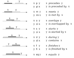
Here are the base relations between two intervals, as timelines.

An images showing base relations between two intervals, as timelines.

SQL did not add all 13 relationships, but we decided that an overlaps predicate would be the most useful.

The result of the <OVERLAPS predicate> is formally defined as the result of the following expression:

(S1 > S2 AND NOT (S1 >= T2 AND T1 >= T2))
 OR (S2 > S1 AND NOT (S2 >= T1 AND T2 >= T1))
 OR (S1 = S2 AND (T1 <> T2 OR T1 = T2))

where S1 and S2 are the starting times of the two time periods and T1 and T2 are their termination times. The rules for the OVERLAPS() predicate sound like they should be intuitive, but they are not. The principles that we wanted in the Standard were:

1. A time period includes its starting point but does not include its end point. We have already discussed this model and its closure properties.

2. If the time periods are not “instantaneous,” they overlap when they share a common time period.

3. If the first term of the predicate is an INTERVAL, and the second term is an instantaneous event (a <datetime> data type), they overlap when the second term is in the time period (but is not the end point of the time period). That follows the half-open model.

4. If the first and second terms are instantaneous events, they overlap only when they are equal.

5. If the starting time is NULL and the finishing time is a <datetime> value, the finishing time becomes the starting time, and we have an event. If the starting time is NULL and the finishing time is an INTERVAL value, then both the finishing and starting times are NULL.

Please consider how your intuition reacts to these results when the granularity is at the YEAR-MONTH-DAY level. Remember that the day begins at 00:00:00 Hrs.

(today, today) OVERLAPS (today, today) = TRUE
 (today, tomorrow) OVERLAPS (today, today) = TRUE
 (today, tomorrow) OVERLAPS (tomorrow, tomorrow) = FALSE
 (yesterday, today) OVERLAPS (today, tomorrow) = FALSE

Contiguous temporal intervals with DDL

Alexander Kuznetsov wrote this idiom for History Tables in T-SQL, but it generalizes to any SQL. It builds a temporal chain from the current row to the previous row with a self-reference. This is easier to show with code:

CREATE TABLE Tasks
(task_id INTEGER NOT NULL,  --  makes sense in your data
 task_score CHAR(1) NOT NULL,  -- whatever makes sense in your data
 previous_end_date DATE, -- null means first task
 current_start_date DATE DEFAULT CURRENT_TIMESTAMP NOT NULL,
 CONSTRAINT previous_end_date_and_current_start_in_sequence
   CHECK (prev_end_date <= current_start_date)
 DEFERRABLE INITIALLY IMMEDIATE,
 current_end_date DATE, -- null means unfinished current task
 CONSTRAINT current_start_and_end_dates_in_sequence
   CHECK (current_start_date <= current_end_date),
 CONSTRAINT end_dates_in_sequence
   CHECK (previous_end_date <> current_end_date),
 PRIMARY KEY (task_id, current_start_date),
 UNIQUE (task_id, previous_end_date), -- null first task
 UNIQUE (task_id, current_end_date), -- one null current task
 FOREIGN KEY (task_id, previous_end_date)  -- self-reference
   REFERENCES Tasks (task_id, current_end_date));

Well, that looks complicated! Let’s look at it column by column. Task_id explains itself. The previous_end_date will not have a value for the first task in the chain, so it is NULL-able. The current_start_date and current_end_date are the same data elements, temporal sequence, and PRIMARY KEY constraints we had in the simple history table schema.

The two UNIQUE constraints will allow one NULL in their pairs of columns and prevent duplicates. Remember that UNIQUE is NULL-able, not like PRIMARY KEY, which implies UNIQUE NOT NULL.

Finally, the FOREIGN KEY is the real trick. Obviously, the previous task has to end when the current task started for them to abut, so there is another constraint. This constraint is a self-reference that makes sure this is true. Modifying data in this type of table is easy but requires some thought.

There is just one little problem with that FOREIGN KEY constraint. It will not let you put the first task into the table. There is nothing for the constraint to reference. In Standard SQL, we can declare constraints to be DEFERABLE with some other options. The idea is that you can turn a constraint ON or OFF during a session so the database can be in a state that would otherwise be illegal. But at the end of the session, all constraints have to be TRUE or UNKNOWN.

When a disabled constraint is re-enabled, the database does not check to ensure any existing data meets the constraints. You will want to hide this in a procedure body to get things started.

BETWEEN

Please notice that the OVERLAPS and BETWEEN predicates work with static intervals, but there are also dynamic predicates for data. The LEAD and LAG operators view the rows as representing points in time or in a sequence, but that is a topic for another article.

If you liked this article, you might also like A UNIQUE experience


The post BETWEEN the two of us appeared first on Simple Talk.


from Simple Talk https://ift.tt/3Dwab6Q
via