Wednesday, May 11, 2022

Buying an SSD card for a grandchild

We recently ordered a tablet for our 8-year-old grandson. We ensured that it would support a decent-sized SSD card, 128 GB, for storing all the photos and videos he will likely take. He’ll mostly play games or watch videos on the tablet, and his favorite video is Dragon’s Doom.

Purchasing this gift made me think about how much has changed over the past 40 years or so. I remember the excitement of buying a 5.25-inch floppy drive and modem for our TI-99/4A back in the early 80s. I caught my first look at BASIC in 1980 on a TRS-80 but figured out how to write a few simple programs on the TI. We wasted spent a lot of time on BBS (The Bulletin Board System) and CompuServe before dial-up internet was available in the 90s. I can still hear that modem connecting!

Our first desktop PC was slow, probably even for that time, as we bought a clearance model. We upgraded it many times during its life and had to use a compression utility to get more drive space. I don’t recall the specs, but the hard drive was probably just a couple of hundred megabytes. These were the 16-bit days, and software arrived with printed books and lots of installation floppies. Around 1995, I purchased a laptop. This was the beginning of always having multiple working computers in the house.

Photography is another example. Taking home photos was once cumbersome and expensive. I had a 126 Kodak Instamatic, and I needed the film cartridge and a sometimes a flashcube to take a photo.  Then, once the film was used up, possibly over several months, it had to be taken in to be developed. Today, most phones are equipped to take digital photos and videos – no film needed.

Speaking of phones, how did we manage to keep track of each other before mobile phones? The chances of catching someone at home at the right time to answer a phone call on a landline seems astronomical, but we did it. A recent science fiction series, Upload, shows the characters using a handphone. There’s no need to carry a phone around as it’s embedded in one’s hand. They also have a 3D instant food printer that prints real meals. I’m not sure which one of these will be available in real life first, but I need that food printer now!

That tiny SSD card that will store my grandson’s photos was unimaginable just a few decades ago. Maybe in 20 years, we will look back at today’s world and wonder how we managed with such primitive technology.

Commentary Competition

Enjoyed the topic? Have a relevant anecdote? Disagree with the author? Leave your two cents on this post in the comments below, and our favourite response will win a $50 Amazon gift card. The competition closes two weeks from the date of publication, and the winner will be announced in the next Simple Talk newsletter.

The post Buying an SSD card for a grandchild appeared first on Simple Talk.


from Simple Talk https://ift.tt/s83o2DU
via

Tuesday, May 10, 2022

How to run Kubernetes clusters locally on Windows

Kubernetes production clusters are typically run on cloud platforms. However, running and deploying Kubernetes applications on cloud platforms such as Google Kubernetes Engine is costly. These high costs can restrict the Kubernetes learning process for beginners. However, running Kubernetes clusters locally helps you efficiently test applications without disrupting the production environment or paying for cloud services. 

To make things easier, the Kubernetes team developed two tools,  Minikube and Kind, that allow Kubernetes users to run clusters locally without spending a dollar. This article will cover how to do it with Kind. Kind is a command-line tool used to run Kubernetes clusters locally on your computer using Docker containers. Kind works with Docker by loading Docker containers into Kind clusters. A Kubernetes cluster is a group of nodes used to run containerized applications.

Kind uses a virtual machine on your pc to create nodes. Kind is also widely used to test and implement continuous integration tasks. Kind runs clusters locally from your computer making it easy to develop your Kubernetes applications without the need for a server.

Kind is good at creating clusters with multiple nodes. The more nodes you have, the more containerized applications you can run. These clusters created by Kind can be operated and interacted with using Kubectl. Kubectl is a command line that enables you to execute commands that communicate with your Kubernetes cluster and make changes.

In this article, you will learn how to install Kind on Windows. In addition, you will learn how to create a cluster using Kind and create a service.

Table of contents

  1. Prerequisites
  2. How to install Kind on Windows
  3. How to create and delete a cluster
  4. How to create a cluster with multiple nodes
  5. How to create a service
  6. How to export cluster logs
  7. Conclusion

Prerequisites

  • A Windows machine that has at least 8GB RAM. Using a machine that has less than 8GB of RAM will raise memory issues and complications when running a Kind cluster.
  • You need to have installed Kubectl before starting this tutorial; if you haven’t installed Kubectl, you install it from here.
  • Kind cannot function without Docker, install Docker from here.
  • In this tutorial, you will install Kind using Chocolatey. Download Chocolatey here.
  • Run Windows PowerShell as an Administrator whenever executing any Kind or Kubectl commands.

How to install Kind on Windows

In this article, you will learn how to download Kubernetes Kind using Chocolatey. Use the following command to download Kind using chocolatey:

choco install kind

Chocolatey will install 6 packages. After Kind has been successfully installed, you will get the list of the installed artifacts:

kb2919355 v1.0.20160915
dotnetfx v4.8.0.20190930
docker-desktop v4.4.4
kb2919442 v1.0.20160915
chocolatey-dotnetfx.extension v1.0.1
kind v0.11.1

To check if Kind has been installed successfully, execute the following command on Powershell:

kind version

If Kind has been installed successfully you will get the version output and your computer’s processor:

kind v0.11.1 go1.16.4 windows/amd64

Now you’re done installing Kind on Windows. You can now start creating clusters locally using kind. If you ever get stuck using Kind, use the command shown below to get all available commands:

kind -h

You will get the following list of commands as output:

Available Commands:
  build       Build one of [node-image]
  completion  Output shell completion code for the specified shell (bash, zsh or fish)
  create      Creates one of [cluster]
  delete      Deletes one of [cluster]
  export      Exports one of [kubeconfig, logs]
  get         Gets one of [clusters, nodes, kubeconfig]
  help        Help about any command
  load        Loads images into nodes
  version     Prints the kind CLI version

Flags:
  -h, --help              help for kind
      --loglevel string   DEPRECATED: see -v instead
  -q, --quiet             silence all stderr output
  -v, --verbosity int32   info log verbosity
      --version           version for kind

Use the -h flag to get more information about any command. For example, executing this command:

kind build -h

gives you the following detailed information about the build command:

Usage:
kind build [flags]
kind build [command]

Available Commands:
node-image Build the node image

Flags:
-h, --help help for build

Global Flags:
--loglevel string DEPRECATED: see -v instead
-q, --quiet silence all stderr output
-v, --verbosity int32 info log verbosity

Use "kind build [command] --help" for more information about a command.

How to create and delete a cluster

Clusters are the holy grail of Kubernetes. Clusters comprise containers with all the runtime resources needed to run applications in different operating systems.

Use the following command to create a default Kind cluster:

kind create cluster

The above command will create a default cluster called kind. If you want to use a specific name, add the --name flag to the kind create cluster command. Here is an example:

kind create cluster --name simple-cluster

The Kind create command has the following arguments and options

  • --quiet: this flag silences all stderr output.
  • --verbosity int32: This flag will log verbosity information.

When your cluster has been created successfully, you will get the following output:

Creating cluster "simple-cluster" ...
• Ensuring node image (kindest/node:v1.21.1) 🖼 ...
✓ Ensuring node image (kindest/node:v1.21.1) 🖼
• Preparing nodes 📦 ...
✓ Preparing nodes 📦
• Writing configuration 📜 ...
✓ Writing configuration 📜
• Starting control-plane 🕹 ...
✓ Starting control-plane 🕹
• Installing CNI 🔌 ...
✓ Installing CNI 🔌
• Installing StorageClass 💾 ...
✓ Installing StorageClass 💾
Set kubectl context to "kind-simple-cluster"

After you have created your cluster, use the following command to check if the cluster has been created successfully or get the list of all Kind clusters running:

kind get clusters

If you want to interact with a specific cluster locally. Use the following command and specify the name of the cluster (kind-<cluster-name>):

kubectl cluster-info --context kind-simple-cluster

You will get the following output which shows you where the Kubernetes control plane and CoreDNS are running at:

Kubernetes control plane is running at https://127.0.0.1:2450
CoreDNS is running at https://127.0.0.1:2450/api/v1/namespaces/kube-system/services/kube-dns:dns/proxy

The cluster’s configuration access will be stored in the ${HOME}/.kube/config file. This file acts as your cluster’s manifest. Here is the configuration access of the default Kind cluster created earlier:

apiVersion: v1
clusters:
- cluster:
    certificate-authority-data:
    server: https://127.0.0.1:2474
  name: kind-kind
contexts:
- context:
    cluster: kind-kind
    user: kind-kind
  name: kind-kind
current-context: kind-kind
kind: Config
preferences: {}
users:
- name: kind-kind
  user:
    client-certificate-data:
    client-key-data:

A corresponding Docker container will be created automatically when creating a Kind cluster. Use the following docker command to see the corresponding docker container:

docker ps

You will get the following information:

CONTAINER ID: 22add82af339
IMAGE: kindest/node:v1.21.1
COMMAND:"/usr/local/bin/entr..."
CREATED: About an hour ago
STATUS: Up About an hour
PORTS: 127.0.0.1:2450->6443/tcp NAMES:simple-cluster-control-plane

To view nodes created by the cluster, use the following command to view them:

kubectl get nodes

You will get the following information:

NAME                         STATUS ROLES               AGE VERSION
simple-cluster-control-plane Ready control-plane,master 89m v1.21.1

Use the following command to delete a cluster:

kind delete cluster

After the cluster has been successfully deleted, you will get the following information:

Deleting cluster "kind" ...

To delete a cluster without the default name, use the –name flag.

How to create a cluster with multiple nodes

A Kubernetes node is a virtual machine that runs a cluster. There are two types of nodes which are:

  • Worker node: A worker node executes and runs applications and containers assigned to it.
  • control-plane: A control-plane controls all the worker nodes.

You’ll need a YAML file that defines the nodes when creating a multi-node cluster.

A node can also be a physical machine. To add more nodes to your cluster, start by creating a cluster and adding different roles of nodes you want to add to your cluster. Save the following in kind-config.yaml.

kind: Cluster
apiVersion: kind.x-k8s.io/v1alpha4
nodes:
- role: control-plane
- role: worker
- role: worker

After saving the YAML file that has the above contents. Use the following command to apply changes:

kind create cluster --name best-cluster --config kind-config.yaml

You will get the following output; this time the output will show that Kind is creating multiple nodes and show that it is joining worker nodes at the bottom of the output:

Creating cluster "best-cluster" ...
• Ensuring node image (kindest/node:v1.21.1) 🖼 ...
✓ Ensuring node image (kindest/node:v1.21.1) 🖼
• Preparing nodes 📦 📦 📦 ...
✓ Preparing nodes 📦 📦 📦
• Writing configuration 📜 ...
✓ Writing configuration 📜
• Starting control-plane 🕹 ...
✓ Starting control-plane 🕹
• Installing CNI 🔌 ...
✓ Installing CNI 🔌
• Installing StorageClass 💾 ...
✓ Installing StorageClass 💾
• Joining worker nodes 🚜 ...
✓ Joining worker nodes 🚜

Set kubectl context to "kind-best-cluster"

You can now use your cluster with:

kubectl cluster-info --context kind-best-cluster
Thanks for using kind! 😊

To check if the nodes have been created successfully and are ready, execute the following command:

kubectl get nodes

You will get the following output:

NAME                       STATUS   ROLES                AGE   VERSION
best-cluster-control-plane Ready    control-plane,master 4m59s v1.21.1
best-cluster-worker        NotReady <none>               90s   v1.21.1
best-cluster-worker2       NotReady <none>               90s   v1.21.1

How to create a service

A Kubernetes service is used to expose your cluster and connect with authorized traffic outside your cluster. An ingress controller is a type of load balancer service that routes traffic to your service.

The following YAML file creates a pod, service, and the ingress controller objects. The service will receive traffic through the 5678 port. The ingress controller version is set to networking.k8s.io/v1.

Start by creating a YAML file that will define and configure the service. Add the following content to the YAML file:

kind: Pod
apiVersion: v1
metadata:
  name: best-cluster
  labels:
    app: best-cluster
spec:
  containers:
  - name: best-cluster
    image: hashicorp/http-echo:0.2.3
    args:
    - "-You just deployed your first service"
---
kind: Service
apiVersion: v1
metadata:
  name: simple-service
spec:
  selector:
    app: best-cluster
  ports:
  # Default port used by the image
  - port: 5678
---
apiVersion: networking.k8s.io/v1
kind: Ingress
metadata:
  name: simple-ingress
spec:
  rules:
  - http:
      paths:
      - pathType: Prefix
        path: "/simple"
        backend:
          service:
            name: simple-service
            port:
              number: 5678
---

After saving your YAML file, use the following command to deploy the service:

kubectl apply -f simple-service.yaml

Execute the following command to check if the service is running:

kubectl get services

You will get the following output:

NAME              TYPE      CLUSTER-IP    EXTERNAL-IP   PORT(S)  AGE
kubernetes        ClusterIP 10.96.0.1     <none>        443/TCP  72m
simple-service    ClusterIP 10.96.245.41  <none>        5678/TCP 56s

The above output shows that your cluster is now ready to receive traffic from outside the cluster through the service you just created.

How to export cluster logs

Kubernetes logs give you visibility on how your cluster performs. Some vulnerabilities and defects will be identified when inspecting and auditing logs. Kind has the following command that is used to export cluster logs to your desired directory on your pc:

kind export logs C:\Users\redgate

The above command will give you the following output, exporting logs of the default cluster. Use the –name flag if you have named the cluster something else:

Exporting logs for cluster “kind” to:
C:\Users\redgate

The structure of the logs will look like this in the folder you exported them to

├── docker-info.txt
└── kind-control-plane/     
         ├── containers     
         ├── docker.log     
         ├── inspect.json     
         ├── journal.log     
         ├── kubelet.log     
         ├── kubernetes-
version.txt
        └── pods/

Conclusion

In this article you have learned:

  1. How to install Kind on Windows.
  2. How to create a cluster using Kind.
  3. How to create a cluster with multiple nodes.
  4. How to create a service.

The above skills are enough to get you started with the journey of creating Kubernetes clusters using Kind. You can advance your Kubernetes skills on the Kubernetes official page here.


The post How to run Kubernetes clusters locally on Windows appeared first on Simple Talk.


from Simple Talk https://ift.tt/29nW1CD
via

Monday, May 9, 2022

Working with MySQL stored functions

The series so far:

  1. Getting started with MySQL
  2. Working with MySQL tables
  3. Working with MySQL views
  4. Working with MySQL stored procedures
  5. Working with MySQL stored functions

In the previous three articles in this series, I focused on creating basic database objects that you can use to get started with MySQL. You learned how to build an initial database and then add tables, views, and stored procedures. In this article, I cover one more important type of object, the stored function, a routine that is stored in a database and can be invoked on-demand, similar to a user-defined scalar function in SQL Server or other database systems.

Stored functions work much like MySQL built-in functions. You can call either type of function in an expression, such as those in a query’s SELECT, WHERE, or ORDER BY clause. For example, you might use the CAST built-in function in a SELECT clause to convert a column to a different data type, as in CAST(plane_id AS CHAR). The expression converts the plane_id column (an integer) to a character data type. In the same way, you can use a stored function in your expression, applying your own logic to the plane_id column or any other column.

Before I go any further with stored functions, it’s important to note that there are three different types of MySQL functions that you can add at the database or server level:

  • Stored functions. Functions that you create as database objects by using the CREATE FUNCTION statement.
  • Loadable functions. Functions that are compiled as library files and then loaded to the server dynamically by running a CREATE FUNCTION statement.
  • Native functions. Functions that are added to the server by modifying the MySQL source code and compiling it into mysqld.

This article focuses on creating stored functions, which share many of the same characteristics as MySQL stored procedures. In fact, I had considered writing about both of them in the previous article, but I think there are enough differences between them to warrant a separate article. It also provides a more consistent way of introducing each of the primary MySQL object types, even if it does mean repeating some of the information. With this in mind, let’s get started with the stored function.

Preparing your MySQL environment

As with the previous few articles, the examples in this article are based on the travel database. If you already have it installed, you can skip this section. If not, you can start by running the following SQL script to create the database and its tables:

DROP DATABASE IF EXISTS travel;
CREATE DATABASE travel;
USE travel;
CREATE TABLE manufacturers (
  manufacturer_id INT UNSIGNED NOT NULL AUTO_INCREMENT,
  manufacturer VARCHAR(50) NOT NULL,
  create_date TIMESTAMP NOT NULL DEFAULT CURRENT_TIMESTAMP,
  last_update TIMESTAMP NOT NULL 
    DEFAULT CURRENT_TIMESTAMP ON UPDATE CURRENT_TIMESTAMP,
  PRIMARY KEY (manufacturer_id) ) 
ENGINE=InnoDB AUTO_INCREMENT=1001;
CREATE TABLE airplanes (
  plane_id INT UNSIGNED NOT NULL AUTO_INCREMENT,
  plane VARCHAR(50) NOT NULL,
  manufacturer_id INT UNSIGNED NOT NULL,
  engine_type VARCHAR(50) NOT NULL,
  engine_count TINYINT NOT NULL,
  max_weight MEDIUMINT UNSIGNED NOT NULL,
  wingspan DECIMAL(5,2) NOT NULL,
  plane_length DECIMAL(5,2) NOT NULL,
  parking_area INT GENERATED ALWAYS AS 
        ((wingspan * plane_length)) STORED,
  icao_code CHAR(4) NOT NULL,
  create_date TIMESTAMP NOT NULL DEFAULT CURRENT_TIMESTAMP,
  last_update TIMESTAMP NOT NULL 
    DEFAULT CURRENT_TIMESTAMP ON UPDATE CURRENT_TIMESTAMP,
  PRIMARY KEY (plane_id),
  CONSTRAINT fk_manufacturer_id FOREIGN KEY (manufacturer_id) 
    REFERENCES manufacturers (manufacturer_id) ) 
ENGINE=InnoDB AUTO_INCREMENT=101;

The airplanes table includes a foreign key that references the manufacturers table, so be sure to create the tables in the order shown here. After you create the tables, you can add sample data to them so you’ll be able to test your function. To populate the tables, run the following INSERT statements:

INSERT INTO manufacturers (manufacturer)
VALUES ('Airbus'), ('Beechcraft'), ('Piper');
INSERT INTO airplanes 
  (plane, manufacturer_id, engine_type, engine_count, 
    max_weight, wingspan, plane_length, icao_code)
VALUES 
  ('A380-800', 1001, 'jet', 4, 1267658, 261.65, 238.62, 'A388'),
  ('A319neo Sharklet', 1001, 'jet', 2, 166449, 117.45, 111.02, 'A319'),
  ('ACJ320neo (Corporate Jet version)', 1001, 'jet', 2, 174165, 
               117.45, 123.27, 'A320'),
  ('A300-200 (A300-C4-200, F4-200)', 1001, 'jet', 2, 363760, 147.08, 
               175.50, 'A30B'),
  ('Beech 390 Premier I, IA, II (Raytheon Premier I)', 1002, 'jet', 
               2, 12500, 44.50, 46.00, 'PRM1'),
  ('Beechjet 400 (from/same as MU-300-10 Diamond II)', 1002, 'jet', 
              2, 15780, 43.50, 48.42, 'BE40'),
  ('1900D', 1002, 'Turboprop', 2,17120,  57.75, 57.67, 'B190'),
  ('PA-24-400 Comanche', 1003, 'piston', 1, 3600, 36.00, 24.79, 'PA24'),
  ('PA-46-600TP Malibu Meridian, M600', 1003, 'Turboprop', 1, 6000, 
         43.17, 29.60, 'P46T'),
  ('J-3 Cub', 1003, 'piston', 1, 1220, 38.00, 22.42, 'J3');

As with the CREATE TABLE statements, you should run the INSERT statements in the order specified here so you don’t violate the foreign key defined on the airplanes table. Once you have the tables set up and populated, you can start creating stored functions.

Creating a stored function in MySQL

To add a stored function to a MySQL database, you can use the CREATE FUNCTION statement. The statement is similar to a CREATE PROCEDURE statement in several respects. In both cases, you must provide a name for the object and you must define a routine. You also have the option to include a DEFINER clause, one or more characteristics, and one or more parameters.

Despite these similarities, the CREATE FUNCTION statement differs in several important ways:

  • A stored function can return only one value, unlike a stored procedure, which can return multiple values or an entire result set.
  • A stored function supports input parameters only. A stored procedure supports IN, OUT, and INOUT parameters in any combination.
  • A stored function must include a RETURNS clause in its definition before the routine. The clause specifies the data type for the function’s returned value. Stored procedures do not support this clause.
  • A stored function’s routine must include a RETURN statement that specifies the function’s returned value. The routine does not have to include any other statements, only the RETURN statement. If it does include other statements, only the RETURN statement can return a value.

With these guidelines in mind, let’s look at a simple example of a CREATE FUNCTION statement, which defines a stored function that converts pounds to kilograms:

DELIMITER //
CREATE FUNCTION lbs_to_kg(lbs MEDIUMINT UNSIGNED)
RETURNS MEDIUMINT UNSIGNED 
DETERMINISTIC
BEGIN
  RETURN (lbs * 0.45359237);
END//
DELIMITER ;

The function is named lbs_to_kg and includes one input parameter named lbs. You do not have to include a parameter when defining a function, but typically you’ll want at least one. If you add more than one, you need to separate them with commas.

The parameter definition is enclosed in parentheses and includes the parameter’s data type, MEDIUMINT UNSIGNED. I chose this data type because I ultimately want to use the function for the max_weight column in the airplanes table, which is also defined with that data type.

In addition, I used the MEDIUMINT UNSIGNED data type for the RETURNS clause. The clause specifies that the function’s returned value should be an integer in the range permitted by this data type. I figured we were safe with this data type because one pound is equivalent to 0.45359237 kilograms, so the returned value would never exceed the maximum value in the max_weight column.

If you want to support a greater range of values, you can instead use the INT or BIGINT data type for the lbs parameter and the RETURNS clause. This would provide you with more flexibility should you want to use the function to convert values that exceed those in the max_weight column.

The RETURNS clause is followed by the DETERMINISTIC characteristic. A characteristic is one of several options that can be added to a function definition, each one affecting the function in a different way. For example, you can add a characteristic to indicate the routine language or to define the routine’s nature. These are the same characteristics available to stored procedures.

The DETERMINISTIC characteristic indicates that the function will return the same results for the same input parameter each time the function runs. By default, a function is considered nondeterministic unless specified otherwise. Using the DETERMINISTIC characteristic can help the optimizer make better execution plan choices. However, assigning the characteristic to a nondeterministic function could cause the optimizer to make incorrect choices.

The function’s routine comes after the listed characteristics. For this routine, I’ve used the BEGIN…END syntax to set up a compound statement, even though there is only one RETURN statement. Often your routine will include a compound statement—a block of one or more SQL statements—and I wanted to be sure you understood how to include them in your function definition. As with stored procedures, it’s not uncommon for developers to use a compound statement, even if it includes only a single SQL statement.

The RETURN statement defines a simple mathematic expression that multiples the lbs input parameter value by 0.45359237 to arrive at the number of kilograms for the specified weight. The result from this calculation is what is returned by the function when you run it.

The preceding example also includes two DELIMITER statements that surround the function definition. The first DELIMITER statement changes the delimiter to double forward slashes (//), and the second DELIMITER statement changes the delimiter back to a semi-colon (the default). As you saw in the previous article, this provides a way to pass the entire function definition to the server as a single statement.

Verifying a newly created stored function

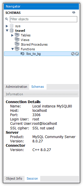
After you run the CREATE FUNCTION statement, you can verify that it’s been added to the travel database by viewing it in Navigator, as shown in Figure 1. (You might need to refresh Navigator to see the new function.)

An image showing the Navigator. The lbs_to_kg function can be seen in the Functions folder

Figure 1. Viewing the function in Navigator

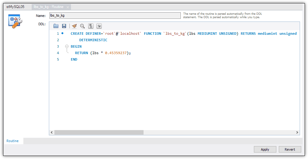
From Navigator, you can open the function definition in the Routine tab by clicking the wrench icon next to the function name. Figure 2 shows the function definition on the Routine tab. The CREATE FUNCTION statement is nearly identical to what you created, except that it now includes the DEFINER clause after the CREATE keyword.

An image showing the function definition in the dialog. CREATE DEFINER='root'@'localhost' FUNCTION 'lbs_to_kg'(lbs MEDIUMINT UNSIGNED) RETURNS mediumint unsigned DETERMINISTIC BEGIN RETURNS (lbs * 0.45359237); END

Figure 2. Viewing the function definition on the Routine tab

As you saw with views and stored procedures, the DEFINER clause specifies which account has been designated as the object creator. I ran the CREATE FUNCTION statement when I was signed in under the root account on my local MySQL instance, so that’s the username added to the definition. By default, MySQL uses the account of the user who runs the CREATE PROCEDURE statement, but you can specify a different account as long as it’s been granted adequate permissions.

You might have noticed that the function definition on the Routine tab does not include the DELIMITER statements or custom delimiter. However, if you were to update the definition and click Apply, Workbench would add those elements for you. (It would also add a DROP PROCEDURE statement that needs to run before the CREATE FUNCTION statement.)

Another way you can verify that the function has been created is to query the routines view in the INFORMATION_SCHEMA database:

SELECT * FROM information_schema.routines
WHERE routine_schema = 'travel';

The results should include the lbs_to_kg function, along with any other stored functions or stored procedures that have been created in the database. If you’re using the setup from the last article, your database might include the get_plane_info stored procedure.

In the preceding example, I included a WHERE clause that limits the results to the travel database. However, you can further limit the results by also specifying the function name in the WHERE clause and by specifying which column or columns to return. For example, the following SELECT statement limits the results to the routine_definition column and to the lbs_to_kg function in the travel database:

SELECT routine_definition
FROM information_schema.routines
WHERE routine_schema = 'travel'
  AND routine_name = 'lbs_to_kg';

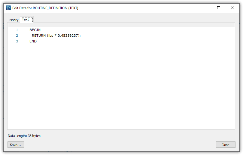
The statement should now return only a single value, although it might be difficult to read. As you saw with stored procedures, you can view a value in its entirety in a separate window. Right-click the value directly in the results and click Open Value in Viewer. MySQL launches a window that displays the value, as shown in Figure 3. (Select the Text tab if it’s not already selected.)

An image showing the full definition of the function in a dialog. BEGIN RETURN (lbs * 0.45359237); END

Figure 3. Examining the function’s routine body in Viewer

As you can see, the window displays only the function’s routine body, which in this case, is a compound statement that includes a RETURN statement.

Using a stored function in a MySQL query

After you verify that your function has been created, you should check that it works as expected. One way to do this is to create a simple SELECT statement that does nothing but call the lbs_to_kg function. For example, the following SELECT statement includes only a SELECT clause, and that clause contains only one expression:

SELECT lbs_to_kg(132) AS max_kg;

The expression calls the lbs_to_kg function, passing in 132 as the parameter value. The expression also provides a name for the output column (max_kg). The statement should return a value of 60.

In many cases, you’ll want to use your stored function for more than just running it in a simple SELECT statement. For example, you can use a stored function to transform or augment a column’s values when retrieving data, which is what I’ve done in the following SELECT statement:

SELECT a.plane, max_weight AS max_lbs, 
  lbs_to_kg(max_weight) AS max_kg
FROM airplanes a INNER JOIN manufacturers m
  ON a.manufacturer_id = m.manufacturer_id
WHERE m.manufacturer = 'airbus'
ORDER BY a.plane;

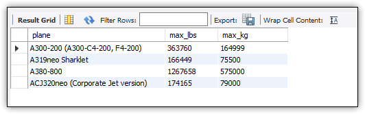
The statement joins the airplanes and manufacturers tables based on the manufacturer_id column in each table. The statement’s SELECT clause includes an expression that uses the lbs_to_kg function to convert the max_weight column to kilograms and return a column named max_kg. The statement returns the results shown in Figure 4.

An image showing the results of running the query. Four rows returned. Plane, max_lbs, max_kg. In each row the lbs has been translated into kg

Figure 4. Using the stored function in your query

The results include the original weight (in pounds) in the max_lbs column and the weight in kilograms in the max_kg column after converting the max_weight values. By including both weights, you can quickly compare them to get a general sense of whether the function seems to be returning the expected results.

Updating a stored function in MySQL

As pointed out earlier, MySQL stored functions are similar to stored procedures in several ways. For example, they both support characteristics, input parameters, and the DEFINER clause. They’re also similar in another important way. You can alter only the characteristics. You cannot change the routine or any other statement elements. Instead, you must first drop the function and then re-create it, incorporating any new elements.

To drop a stored function, you can use the DROP FUNCTION statement, as shown in the following example:

DROP FUNCTION IF EXISTS lbs_to_kg;

The IF EXISTS clause is optional, but it’s a handy way to avoid generating errors when you try to drop a function. The clause can be particularly useful when you’re developing your database schema and you’re regularly updating the objects.

After you’ve dropped the function, you can modify the definition to meet your new requirements. For example, the following CREATE FUNCTION statement re-creates the lbs_to_kg function but this time adds a DECLARE statement and an IF construction to the compound statement:

DELIMITER //
CREATE FUNCTION lbs_to_kg(lbs MEDIUMINT UNSIGNED)
RETURNS VARCHAR(50) 
DETERMINISTIC
BEGIN
  DECLARE msg VARCHAR(50);
  IF lbs > 999999 THEN SET msg = 
    CONCAT(ROUND((lbs * 0.45359237), 0), 
            ' kg exceeds airport weight limits.');
  ELSEIF lbs >= 100000 AND lbs <= 999999 THEN SET msg = 
    CONCAT(ROUND((lbs * 0.45359237), 0), 
            ' kg exceeds runway weight limits.');
  ELSE SET msg = CONCAT(ROUND((lbs * 0.45359237), 0), 
            ' kg within weight limits.');
  END IF;
  RETURN msg;
END//
DELIMITER ;

The DECLARE statement declares the msg local variable and assigns it the VARCHAR data type. Notice that the RETURNS clause has also been updated to the VARCHAR data type to match the msg variable. The variable can then be used in the final RETURN statement to provide the function’s output value.

The compound statement also includes an IF statement. The statement starts with an initial conditional clause, which is followed by an ELSEIF clause and then an ELSE clause. Each clause implements the same logic based on the value of the lbs input parameter. If the lbs value falls within the specified range, the msg variable is set to a predefined value based on that range. (We’ll be covering conditional statements in more detail later in the series.)

The msg value is determined first by converting the lbs value to kilograms and then concatenating the results with a string (the message body). For example, if the lbs value is greater than 99999, the msg variable is set to the number of kilograms plus the message ‘ kg exceeds the airport weight limits.’

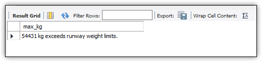
To help carry out this logic, each conditional clause also includes two built-in functions: ROUND and CONCAT. The ROUND function rounds the calculated kilograms to a whole number, and the CONCAT function concatenates the rounded kilograms with the specified text. For example, if the weight in pounds is 120,000, the IF statement will set the msg variable to ‘54431 kg exceeds runway weight limits.’ You can see this for yourself by running the following SELECT statement:

SELECT lbs_to_kg(120000) AS max_kg;

The statement should return the results shown in Figure 5.

An image showing the results of the query. max_kg 54431 kg exceeds the runway weight limits

Figure 5. Viewing the results returned by the updated stored function

You can also use the lbs_to_kg function in a more elaborate SELECT statement, just like you did earlier:

SELECT m.manufacturer, a.plane, 
  max_weight AS max_lbs, 
  lbs_to_kg(max_weight) AS max_kg
FROM airplanes a INNER JOIN manufacturers m
  ON a.manufacturer_id = m.manufacturer_id
ORDER BY m.manufacturer, a.plane;

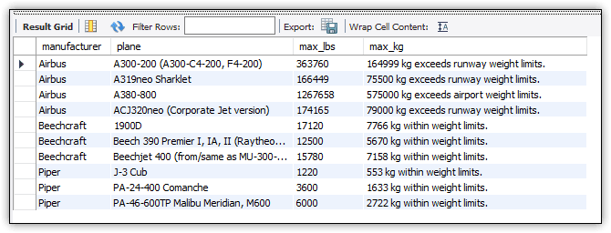
Now each returned row includes one of the three messages in the max_kg column. The message is based on the number of pounds in the max_weight column, which is passed to the function through its parameter. Figure 6 shows the results returned by the SELECT statement.

An image showing the results of the query. One row for each plan is returned with the appropriate message that translated lbs to kg and then either exceeds runway weight limits, exceeds airport weight limits or within weight limits

Figure 6. Using a stored function in your query expressions

Your function can, of course, include a much more complex routine than what I’ve done here, but these examples should be enough to give you a sense of what you can do with stored functions and how valuable they can be when building your queries.

Altering a stored function in MySQL

As I mentioned earlier, the only elements of a stored function definition that you can alter are the characteristics. For this, you can use an ALTER FUNCTION statement. For example, the following statement adds a COMMENT characteristic and SQL SECURITY characteristic:

ALTER FUNCTION lbs_to_kg
COMMENT 'converts weight to kilograms and generates message'
SQL SECURITY INVOKER;

The COMMENT characteristic simply adds a comment that describes the function’s purpose. The SQL SECURITY characteristic instructs MySQL to run the routine under the security context of the user account that invokes the function rather than using the definer account (the default behavior).

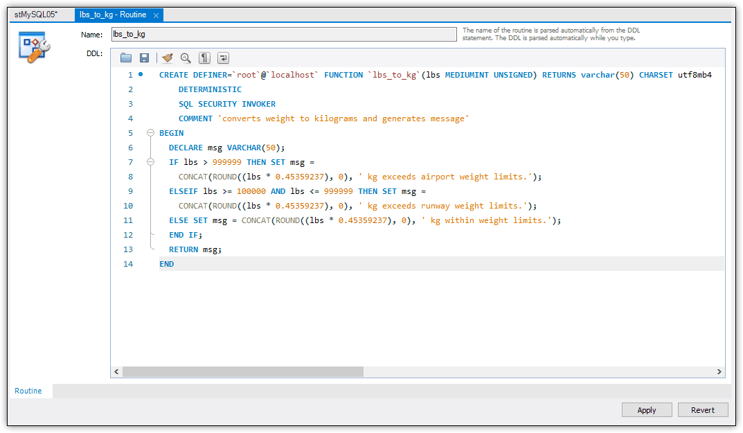
After you run the ALTER FUNCTION statement, you can verify that the characteristics have been added by viewing the function definition on the Routine tab, as shown in Figure 7.

An images showing the new function definition in a dialog

Figure 7. Viewing the stored function definition on the Routine tab

The CREATE PROCEDURE statement now includes three characteristics—the one you added originally and the two you added when you ran the ALTER FUNCTION statement.

Working with stored functions in MySQL

Although stored functions are similar to stored procedures, they serve a distinctly different purpose: to return a value that can be used by an expression during its evaluation. For this reason, stored functions can be extremely useful and are well worth adding to your arsenal of tools, especially since they’re so easy to create and execute. However, they can also impact performance if not carefully implemented. For example, if your query returns thousands of rows of data, an overly complex function could bring your system to its knees as MySQL tries to apply the logic to each row. When used properly, however, stored functions can be incredibly beneficial, especially as you become more adept at building SQL queries.


The post Working with MySQL stored functions appeared first on Simple Talk.


from Simple Talk https://ift.tt/VatPLin
via

Friday, May 6, 2022

The benefits of database change management

Using a change management system, sometimes called source control or version control, is part of the foundation for all the automation required when we begin to build a DevOps process. However, change management brings several additional benefits to the database that make implementing source control within your database systems extremely attractive, all on their own.

The nature of a source control system adds the following functionality:

  • Auditing of the changes made and the source of the change
  • The ability to undo, or rollback, changes to a database without requiring a restore
  • A known state for comparison between environments and tracking changes over time
  • An additional backup of the code that defines the database
  • The isolation of different development processes from each other

To better understand these benefits, let’s address them one at a time.

Auditing

Implementing a change management process within a database immediately adds auditing capabilities that previously were not possible or were very hard to build and maintain. The very nature of most source control systems means that, out of the box, you get auditing capabilities.

The first and most obvious of these is that you’ll be able to tell who made each change. As developers pull their code from the appropriate branch of the source code repository, their changes to that code get recorded within the source control system. Days, weeks, or even years after the fact, you’ll know exactly who made any given change in the code. This capability becomes useful in a number of ways. Obviously, from an audit perspective, knowing who made the change is necessary. However, you’ll also receive the benefits when troubleshooting of being able to talk directly to who made the change to better understand what was done and why. You can also use this as a mechanism for education to ensure that bad or sub-optimal changes to the code can be tracked down to the individual.

Next, you’ll know when the change was introduced to the system. While frequently a problem is immediately apparent, often an issue doesn’t become obvious for days or even weeks. With change management, you can immediately identify when a change was made to assist troubleshooting issues that occur much later.

Finally, you’ll know what the change actually was. Going back to troubleshooting again, it’s frequently difficult to understand if a change was made and what that change was when all you have is the database as it currently exists. Sure, you could restore a copy of the database somewhere to identify the change, but a quick look through the history in source control will be much faster and easier. Then, you can address whatever bug fix is necessary.

Undo

The ability to quickly roll back an individual change is not something available in most database systems. Instead of an undo command, like CTL-Z on a Windows machine, you’re forced to look to backups. When we’re just talking about code, like with a view or a stored procedure, waiting for a very large database to go through a restore process can be extremely time consuming. Instead, in the event of a mistaken change to a piece of code, we can go to the source of the code, our change management system. The ability to quickly undo a mistake makes development much easier and more successful.

Known state

Putting our database code into source control gives us a way to establish exact moments in time. We can see the state of the database as of two weeks ago, despite any development and changes over that intervening period. That ability lends itself to a number of scenarios.

When we want to troubleshoot why behavior has changed, knowing the exact state of all the objects prior to a given change, or even a set of changes, allows us to identify problems more quickly. We can see what was changed, so we can more easily rectify it.

If we have deployed code to a given environment, such as test or pre-production, we can do that from our source control system. Then, we’ll know, just by looking at the source control system, what a given environment’s state is currently. From there, we can decide if we need to deploy new changes or if we’re ready to promote the set of changes defined by our known state to the next environment.

Finally, the known state of a source control system gives us the ability to track changes over time. We can see where we’re making changes to better understand how our systems are being developed. You may even spot trends in sets of changes showing us potential areas for improvement in our processes.

Backups

The ability to restore a given database to a moment in time is a vital part of any recovery process. Building and testing a backup and restore process should be fundamental to any system as a part of the protections built into that system. Change management offers us one more source from which to restore things in the case of an emergency.

Yes, this backup is code only and won’t include all the information stored within our database. However, because this backup is code only, our ability to very quickly restore code from it is much better than what we get from a traditional database restore process. Instead of waiting for an entire database to be restored, you can go directly to the piece of code you need. Further, because we have a history of the changes to that piece of code, you can also go to any one of those historical states as a part of the restore.

Isolation

Releasing that very first version of a piece of code or a database is frequently the easiest part of the process. Difficulties arrive when we must add new functionality or perform hotfixes for problems discovered in our code. Isolating new development from each other and new development from necessary hotfixes is a serious challenge. However, modern change management systems usually use a form of isolation called branching. A branch allows us to create a copy of the code separate from other copies of the code. We can then perform our hotfix in isolation. We’re not impacted by other development going on and can deploy our change independently.

While branching a database will require a copy of that database, branching the code of a database is simple. With this, we can then ensure that two different development streams working on new functionality can perform those tasks without breaking each other’s code. You’ll need to build some testing mechanisms for when those branches get merged back together, but in the meantime, development has not slowed down.

Conclusion

As you can see, there are many benefits from change management within a database. Any or all of these are immediately available to you when you start using a source control system with your database. Then, you can easily leverage this change management system when you later decide that you intend to use it for automating your deployments.


The post The benefits of database change management appeared first on Simple Talk.


from Simple Talk https://ift.tt/wFanuKL
via

Wednesday, May 4, 2022

Combinations, permutations, and derangements

Before I get to the database stuff, here are a few mathematical preliminaries.

Factorials

The factorial function is usually written as (n)!, and it is defined as the product of the first (n) natural numbers. Thus, 5! evaluates to (5 · 4 · 3 · 2 · 1) = 120. As usual, zero becomes a special case, 0! = 1 which can be proven with a slightly different derivation of a factorial. Instead of defining it as a product, define it recursively, like this: n! = CASE WHEN n = 0 THEN 1 ELSE n · (n-1)! END.

Showing the process one step at a time, the recursion unrolls like this:

5! = 5 · 4!
4! = 4 · 3!
3! = 3 · 2!
2! = 2 · 1!
1! = 1 · 0!

Look at the last step of the recursion. Now divide both sides by one to get (1! / 1) = 0! or 1 = 0! Notice that everything done so far is procedural, not set-oriented. RDBMS folks prefer to get away from procedural code. For the rest of this article, you can think of n! as the number of ways to arrange (n) elements of a set into a sequence. Clearly, if you have one element, then you have only one arrangement. But likewise, if you have zero elements, you are also done. Just as you have only one empty set, so you also have only one empty sequence.

Yes, it is possible to define factorials for negative numbers, imaginary numbers, the gamma function for real numbers, and other things. Unless you’re a math major, you will have absolutely no use for any of these fancy tricks. Since SQL is a database language and not a computational one, you might want to use table lookup and not this recursive definition. You can find a table of the numbers one to hundred to populate the table. The factorial function gets big fast!

0! = 1
1! = 1
2! = 2
3! = 6
4! = 24
5! = 120
6! = 720
7! = 5,040
8! = 40,320
9! = 362,880
10! =3,628,800
11! = 39,916,800
12! = 479,001,600

Combinations

Combinations assume there is a set of (n) distinct elements, and you want to get the number of subsets you can pull from this set. There is no concern with exactly what elements go in a particular subset, just the count. The order is not important.

One common notation for this, though not the only notation, is nCr read as Set of (n) things, Choose (r) of them. Notice that (0 ≤ r ≤ n), and that you can choose an empty set. Given a set, the number of subsets in it is 2n ; For example, {a, b, c} has subsets {}, {a}, {b}, {c}, {a, b}, {a, c}, {b, c}, {a, b, c} for total count of 8.

I’ve never understood the term ‘combination locks’ when the order of the numbers that you put into it is very important. Perhaps traditional mechanical security features were not designed by mathematicians.

Permutations

Permutations also assume there is a set of (n) distinct elements, and the goal is to get the number of sequences from this set in any order. However, in this case, the order does matter; (a, b, c) is not the same permutation as (c, b, a).

Derangements

To be honest, I just think that the term ‘derangement’ is really cool. Given two sequences of the same length and with the same data elements, one is a derangement of the other when the data elements do not appear in the same sequence position in the two sequences. For example, (a, b, c) is not a derangement of (c, b, a) because the data element ‘b’ is in the second position in both sequences. Instead, there are two derangements, (c, a, b) and (b, c, a).

A derangement can also be called a permutation with no fixed points. The two notations for derangement of (n) elements are either !(n) or D(n). I find the first one with the leading exclamation point to be a bad choice. It looks too much like a factorial.

The number of derangements of a set with (n) distinct elements is given by the recursive formula : D(n) = (n-1)[D(n-1) + D(n-2)]. If you know D(1) = 0 and D(2) = 1, you can generate subsequent values for D(n). Or you would prefer : D(n) = n D(n-1) + (-1)n?

Obviously, the derangements will be fewer in number than the original permutation.

Derangements of n Elements

D(n)
D(0) = 1
D(1) = 0
D(2) = 1
D(3) = 2
D(4) = 9
D(5) = 44
D(6) = 265
D(7) = 1,854
D(8) = 14,833
D(9) = 133,496
D(10) = 1,334,961
D(11) = 14,684,570
D(12) = 76,214,841

Derangements provide a way to make sure that everyone gets a fair shake when making job assignments. Nobody is stuck in the same job from one assignment cycle to the next. The idea is that eventually, all your personnel would be assigned to every job, but you don’t necessarily know in which assignment cycle any employee will get a particular job.

My favorite use for derangement is when an office does a “Secret Santa” Christmas gift program. If you have never had one of these, the idea is that everyone brings a wrapped gift to work. The gift-giver then picks the name of another employee randomly, and the second employee becomes the recipient. The first rule is that you don’t give a gift to yourself. A second rule is that you’re not supposed to be able to figure out who is the gift giver.

Gift givers are the set, and the recipients are supposed to be an unpredictable derangement. You try doing this by drawing one name at a time, and very quickly a wind up with a situation where only a few possible derangements are left. So much for maintaining secrecy. To get an idea how this works, look at the prior example, with only three data elements in the original permutation. You really need to pick your derangement all at once.

A cute trick for doing this in the real world is to put everybody’s name on a card twice, once on the top and once on the bottom. Shuffle the card deck. Cut the cards in half, leaving the top and bottom halves paired. Take the top half-card from the top halves deck and put it on the bottom of the same top halves deck. Now draw the pairs of cards from the decks, assembling the tops and bottoms to make a new card. The result will be a new card deck with an unpredictable derangement.

Permutations, combinations, and derangements in databases

While all these are interesting, a database person is probably going to be more interested in actually generating the permutations, combinations, and derangements. The problem is that SQL is not really built for this kind of computation. The sets are in databases are in the form of tables, which all have a fixed number of columns. Databases don’t have arrays, link lists, or other data structures, so it’s faked with tables.

If all the columns are the same data element, then this is an example of de-normalizing a table with a repeated group. Here’s a simple example for (n = 3)

CREATE TABLE #Permutations
(c1 INTEGER NOT NULL,
 c2 INTEGER NOT NULL,
 c3 INTEGER NOT NULL,
PRIMARY KEY (c1, c2, c3),
CONSTRAINT Unique_columns
CHECK (
                c1 NOT IN (c2, c3)
                AND c2 NOT IN (c1, c3)
                AND c3 NOT IN (c1, c2)
                
        ));

Remember that all tables must have a key. In these cases, the rows that represent a particular set all have to be unique, and so do all of the columns in that row. This means each row is a key.

The CHECK() constraint ensures that all columns are unique with a row. A lot of the ranges of the dimensions, constraints about membership, etc., in other data structures must be explicitly defined in SQL check constraints. This is one of the many reasons that I tell newbies that 80 to 90% of the work in SQL is done in the DDL, not the DML. Think about trying to write constraints into procedural code for 500 application programs; instead of putting it in one CHECK() constraint, you must duplicate the same code and magically hope that you get it right in every procedural chunk in your system. And when the rules change, you must go back through those 500 pieces of procedural code and update them. Lots of luck with that.

Modeling combinations is easy. Since order doesn’t matter, any simple list of the values will do. That’s a perfect description of a table with one column.

There are several algorithms for generating permutations. Two of the best known are the Heap algorithm (1963) and the Fike algorithm. Both are recursive and are based on the facts that

1) There are n! permutations of the set {1, 2, 3, …,}. This let you know how many times you have to cycle through a loop or how deep your recursion has to go.

2). The next permutation can be generated from the current permutation without fear of duplication.

Robert Sedgwick (you might know from his textbooks that are widely used) wrote a paper on the various methods for generating permutations. He classified them as

1 METHODS BASED ON EXCHANGES
Recursive methods
Adjacent exchanges
Factorial counting
“Loopless” algorithms

2 OTHER TYPES OF ALGORITHMS
Nested cycling
Lexicographic algorithms
Random permutation

References:

https://ift.tt/PiIKvBx

https://ift.tt/znBrXS5. The Computer Journal, vol 19 Issue 2. pages 156-159

https://ift.tt/Ws5mTBw


The post Combinations, permutations, and derangements appeared first on Simple Talk.


from Simple Talk https://ift.tt/bycIQde
via

Monday, May 2, 2022

Optimizing my.cnf for MySQL performance

Since the dawn of software engineering, developers turned to databases to store their data – as time went on, some developers were able to choose their path more clearly: some started using PostgreSQL, some chose MySQL or its flavors (MariaDB or Percona Server), some went for NoSQL-based solutions such as MongoDB.

Those developers that elected to use MySQL, however, quickly noticed that the database management system is not that powerful by default and started searching for ways to improve its performance, security, and high availability beyond its default capabilities; as they found themselves working towards this goal, they found that the answers to the majority of their questions lie in one file – that file was called my.cnf.

What is my.cnf and what does it do?

In order to answer the question how should you optimize your my.cnf file for performance, I’ll start with the basics. The my.cnf file is the main configuration file available within MySQL and all of its flavors. The file contains various parameters that can be configured according to requirements. These parameters will then be loaded onto MySQL as the database management system starts up. There are multiple locations where the my.cnf file could be located (the locations differ depending on what flavor of Linux is used). MySQL usually loads the settings from the file after finding it in one of the following locations:

  • /etc/my.cnf
  • /etc/mysql/my.cnf
  • /var/lib/mysql/my.cnf
  • ~/my.cnf

The path to the directory containing my.cnf can also be defined by changing the value of the MYSQL_HOME variable. If running MySQL on Windows, the directory where the my.ini (note the extension change – my.cnf is called my.ini on Windows) file will be located will correspond to the directory where the MySQL data directory is located. On Linux, it will probably be /var/lib/mysql/my.cnf or in one of the locations specified above. On Windows, the locations will depend on what version of MySQL you’re running – for MySQL 5.7 on Windows 10, for example, the location could be /bin/mysql/mysql*.*.** where *.*.** is the version of the MySQL server or even in the ProgramData directory which is hidden by default. In that case, search for the MySQL folder inside of it.

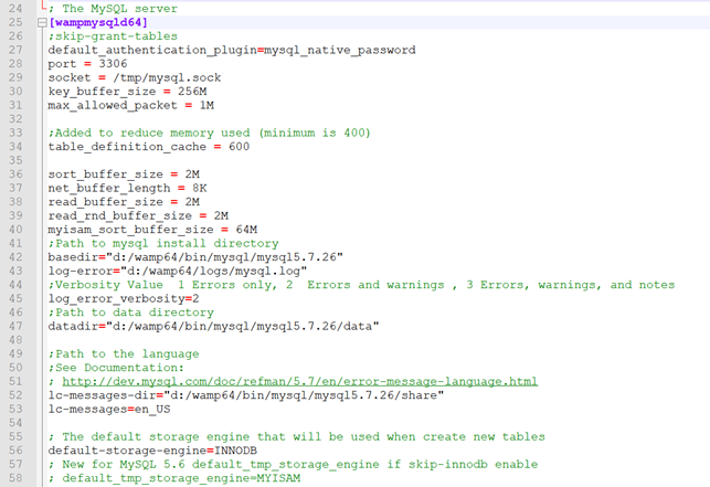
Once opening the my.cnf file, you should see something similar to the following:

Image showing the my.cnf file partial contents.


Image 1 – some of the settings available within my.cnf

As you can see, the file houses a whole lot of parameters – some of those are more crucial for performance, others less. The Windows version of my.cnf (my.ini) is also widely known for the fact that the file includes a bunch of comments (see image above). The Windows version explains pretty much everything, while Linux isn‘t so generous; in many cases, Linux only provides the ‘skeleton’ settings that are most frequently changed and that are related to InnoDB (one of MySQL‘s primary storage engines). One statement is true regardless: to optimize the performance of MySQL, optimize the settings within my.cnf.

Some of you might remember the earlier article about the nuances of indexes in MySQL. That article mentioned that one of the primary storage engines available within MySQL, InnoDB. There are a couple of parameters in the my.cnf file that are crucial for InnoDB’s performance and that need to be optimized to get the best out of MySQL, and the statement rings true for all storage engines available within the database management system. Engineers working with MySQL usually choose the storage engine they want to use according to their needs, modify cnf.ini file to get the best out of the engine, and restart MySQL. Once MySQL is restarted, engineers can enjoy better performance, availability, and, in some cases, security benefits.

How to optimize my.cnf for performance?

When looking at everything from a broader perspective, optimizing my.cnf for performance isn’t that hard. Everything comes down to two things:

  1. Decide what kind of storage engine to use within MySQL.
  2. Optimize the parameters relevant to that storage engine and restart MySQL.

That’s it, really – nothing that complex!

Begin by choosing a storage engine with this table to simplify your choices:

Storage Engine

When to Use?

InnoDB / Percona XtraDB

InnoDB should be chosen when the database supports a general use case software product or if you’re not sure what to use to get the best out of MySQL.

MyISAM

Obsolete storage engine, should only be used if you need the exact row count in a specific table. If used as the main storage engine, MyISAM can become the cause of crashes and lost data.

MEMORY

Such a storage engine stores all data in memory.

CSV

Such a storage engine stores data as CSV files.

MERGE (formerly MRG_MyISAM)

A collection of two or more identical MyISAM-based tables that are supposed to be used as one table.

ARCHIVE

The storage engine is supposed to let us archive data.

FEDERATED

The storage engine lets us access data from a database without using replication or clustering.

BLACKHOLE

The storage engine should be used for testing purposes – all data contained inside of it will be gone in an instant.

EXAMPLE

Should be used as an example of how to build new storage engines.

Despite the plethora of storage engines available for use, most developers and MySQL engineers use InnoDB as it’s widely considered the best for most use cases. Earlier, MyISAM was also a pretty reliable option, but as the storage engine became obsolete due to stability issues and other things, it’s now effectively only suitable for one purpose – knowing the exact count of rows in a table (InnoDB doesn’t provide that information, but MyISAM stores the row count inside of itself.)

Optimizing InnoDB for performance

The InnoDB storage engine has these options, among others, available within my.cnf:

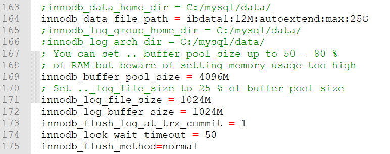
Image showing the innodb section of the my.cnf file. Important settings are innodb_data_file_path, innodb_buffer_pool_size, innodb_log_file_size, innodb_log_buffer_size, innodb_flush_log_at_trx_commit, innodb_lock_wait_timeout, innodb_flush_method

Image 2 – InnoDB parameters within my.cnf

Here’s what the parameters do, one by one:

Parameter

Function

innodb_data_file_path

This parameter depicts the location of the data file (ibdata1) relevant to InnoDB – ibdata1 holds all of the data required for InnoDB to function correctly.

innodb_buffer_pool_size

This parameter outlines the buffer pool size to be used within InnoDB. The buffer pool is used to cache data and indexes of the tables within InnoDB.

innodb_log_file_size

Sets the size of InnoDB log files. The bigger this value is, the less recovery time is needed in case of a crash.

innodb_log_buffer_size

Used to write to the log files.

innodb_flush_log_at_trx_commit

Ways to flush the log when a transaction commits. MySQL offers three values – the default (1) makes InnoDB ACID compliant, while 0 or 2 exchanges ACID for faster write speed.

innodb_lock_wait_timeout

The length of time in seconds a transaction waits for a row lock.

innodb_flush_method

Defines the method used to flush data. The flush method is very important because it can affect I/O throughput. I won’t get into all of your choices here, but keep in mind that MySQL offers a couple of flush methods for you to choose from including, but not limited to:

  • normal which is the default flushing method on Windows. The other option for Windows is unbuffered.
  • fsync which is the default flushing method on Linux – MySQL will use the fsync() function to flush data.
  • O_DIRECT which instructs the operating system to bypass the page cache and perform I/O operations against the disk in Linux.
  • O_DSYNC exchanges speed for consistency – this option is generally faster than O_DIRECT, but data may not be consistent after a crash in Linux.

And here’s how to optimize each of them to get the max out of MySQL when using InnoDB:

  • Set the innodb_data_file_path to extend automatically by specifying autoextend. Some developers might also benefit from the fact that the data file path can also have a maximum size by specifying max after “autoextend” so the parameter looks like this (the maximum size of InnoDB, in this case, is 10GB.):
    innodb_data_file_path = ibdata1:12M:autoextend:max:10G

    If the maximum size is reached, MySQL will return the error:

    ERROR 1114 (HY000): The table is full

  • Set the InnoDB buffer pool size to 50 – 75% of available operating memory on your system. The bigger this parameter is, the faster operations regarding InnoDB (inserts, etc.) will complete.
  • Set the InnoDB log file size to around a quarter (25%) of the InnoDB buffer pool size – the larger the log file size is, the less recovery time you need when restoring MySQL from a crash.
  • It’s advisable to leave the InnoDB log buffer size at the default value of 8MB (8M.)
  • Leave the innodb_flush_log_at_trx_commit at 1 if you want ACID compliance (ACID will ensure that the data remains intact despite any kind of power outages or other failures that could impact data integrity), but switch it to 0 or 2 if you want to exchange ACID for more writing speed. The former will be a fit for most data-related operations, though some infrastructures, especially those dealing with big data sets, might benefit from the exchange.
  • Changing the innodb_lock_wait_timeout value will change how InnoDB responds to a row lock after a specified amount of seconds – the default value for this parameter is 50, meaning that InnoDB will issue an error if a lock is not released after 50 seconds, though this parameter can be modified according to your needs.
  • Most engineers would advise turning the innodb_flush_method to O_DIRECT for MySQL to be able to perform all I/O operations against the disk and bypass the page cache – that way I/O operations should be a lot faster than normal.

These are most of the parameters you need to optimize when using InnoDB. Now, restart MySQL, and the settings will take effect. However, if you elect to use MyISAM instead (perhaps you’re trying out some of its features or using it on an older, not so important server), there are other parameters you should review.

Optimizing MyISAM for performance

If you’re using Windows, scroll down from InnoDB parameters, and you should see four parameters relevant to MyISAM. If you’re a Linux user and you want to use MyISAM for any reason, though, bear in mind that you would probably need to add these parameters in manually:

Parameter

What Does It Do?

key_buffer_size

The equivalent of the InnoDB buffer pool size – it’s recommended to set this value to approximately 40% of the available memory on the server.

myisam_sort_buffer_size

Defines the size of the buffer that is allocated when sorting operations are performed. Raising this parameter from its default value might help with improving the performance of ORDER BY and GROUP BY operations – other than that, this parameter is important when creating indexes or repairing tables.

read_buffer_size

Defines the size of the buffer that is allocated for each thread that does a full table scan (when a database is finding a value by reading the table in sequential order.)

read_rnd_buffer_size

This parameter is used for some sorting operations in order to read rows after sorting is accomplished. The parameter can be used by all tables, not only MyISAM – head over to the documentation for more information.

Other parameters within my.cnf

Once you have optimized either (or both) InnoDB and MyISAM for performance, you can also look a little into other parameters available to be configured within my.cnf.

Parameter

Importance

skip-federated

Leaving this parameter inside of my.cnf without any value (or including this parameter inside of the file) disables the FEDERATED storage engine within MySQL.

secure_file_priv

This parameter defines the directory from where files can be loaded into MySQL when using the LOAD DATA INFILE command – if the wrong directory is specified, MySQL will respond with an error.

sql_mode

This parameter can be used to set the SQL mode to use when MySQL is running. For example, the “ANSI” parameter changes MySQL’s behavior to behave like standard SQL, including “ALLOW_INVALID_DATES” will disable the checking of dates while specifying no value will set the SQL mode to strict. Refer to the documentation for further explanation.

skip-ssl or ssl

The “skip-ssl” option enables MySQL to use an unencrypted connection. The “ssl” option, on the other hand, will specify the fact that MySQL will attempt to connect via SSL and fail if a secure connection cannot be established.

datadir

Defines the location of the data directory of MySQL. Can be redefined – redefining this parameter can be useful for security reasons, though not much apart from that.

log-error

Defines the location of the error log file within MySQL. The location of the error log file can be changed using this parameter, though doing so could be considered “security through obscurity.”

default-storage-engine

Defines the default storage engine used by MySQL.

lc-messages-dir and lc-messages

Some of the more interesting parameters dealing with error messages. The former defines the location of the directory containing language files to be used within MySQL when errors are encountered, while the latter defines the language of the error messages. Redefining these parameters might be very useful for MySQL installation is used by those who cannot speak English or for other reasons.

The given table should give you a rough idea of just how powerful my.cnf really is. Not only can it be used to improve performance for various storage engines, including InnoDB and MyISAM, but the parameters contained within the file are also very useful to complete various kinds of operations. One thing shouldn’t be forgotten, though – whenever you change the values of any parameter contained inside of my.cnf, you should restart the server to be sure that your changes have taken effect.

Optimizing my.cnf for MySQL performance

I hope this article has given you an idea of what a powerful beast my.cnf can be when used properly. The parameters within my.cnf are frequently used to improve the performance of various storage engines as well as queries, they can be used to set up replication and make MySQL capable of doing various kinds of other things. I hope that this article has helped you learn how you should use the parameters within my.cnf to adjust MySQL and make it perform better than before. Make sure to take the advice in this article into account and test the waters before performing any actions on a production server, and I’ll see you in the next one!

The post Optimizing my.cnf for MySQL performance appeared first on Simple Talk.


from Simple Talk https://ift.tt/okh5prI
via

Template for automating Power BI Refresh

I wrote before about Automating table Refresh in Power BI. On that article I explained how to schedule a refresh script using the Azure Automation Account.

We can improve the automation process even more. If we create a parameterized Powershell script and publish it to github, the script becomes available in the Automation Account gallery. You can use it as many times as you wish, scheduling many different administrative tasks in Power BI using XMLA scripts.

The script will be like this one:

<#
.SYNOPSIS
Indexes tables in a database if they have a high fragmentation
.DESCRIPTION
This runbook indexes all of the tables in a given database if the fragmentation is
above a certain percentage.
It highlights how to break up calls into smaller chunks,
in this case each table in a database, and use checkpoints.
This allows the runbook job to resume for the next chunk of work even if the
fairshare feature of Azure Automation puts the job back into the queue every 30 minutes
.PARAMETER PowerBIEndpoint
Power BI XMLA endpoint address
.PARAMETER ServicePrincipal
Service principal to connect to the XMLA endpoint in the format Appid@TenantId
.PARAMETER ServicePrincipalSecret
Secret value created for the service principal
.PARAMETER Query
XMLA statement to be executed, either in XML or JSON.
.NOTES
AUTHOR: Dennes Torres
LASTEDIT: March 20, 2022
#>
param(
[parameter(Mandatory=$True)]
[string] $PowerBIEndpoint,

[parameter(Mandatory=$True)]
[string] $ServicePrincipal,

[parameter(Mandatory=$True)]
[string] $ServicePrincipalSecret,

[parameter(Mandatory=$False)]
[string] $Query

)

$assemblyPath = "C:\Modules\User\Microsoft.AnalysisServices.AdomdClient\Microsoft.AnalysisServices.AdomdClient.dll"
try {Add-Type -Path $assemblyPath}
catch { $_.Exception.LoaderExceptions }

$Connection = New-Object Microsoft.AnalysisServices.AdomdClient.AdomdConnection
$Connection.ConnectionString = "Datasource="+ $PowerBIEndpoint +";User ID="+ $ServicePrincipal
        +";Password="+ $ServicePrincipalSecret
$Command = $Connection.CreateCommand();
$Command.CommandTimeout = 20000;
$Command.CommandType = [System.Data.CommandType]::Text;
$Command.CommandText = $Query;
$Connection.Open()

$Command.ExecuteNonQuery()

$Connection.Close()
$Connection.Dispose()


You can read about how to contribute to the Automation Gallery here. I also wrote about this when I was explaining about a script to re-index SQL Server Tables (published to the automation gallery).

Let’s follow some steps to schedule the script from the gallery in an automation account.

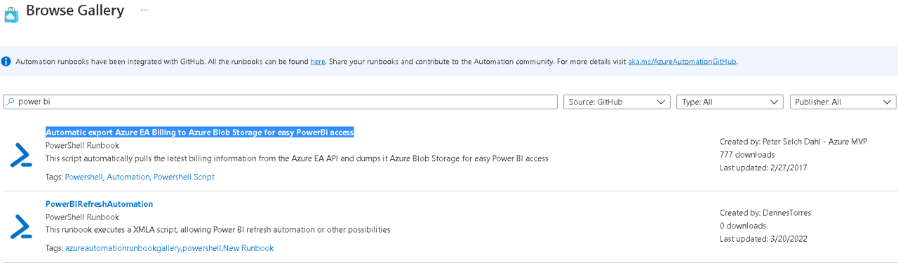
1) In an automation account,  click the Browse Gallery button and search for Power BI. You will find the script I published, as illustrated on the image below.


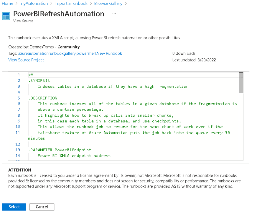
2) Click on the script and you will be able to see the entire code. You can decide if you will import it to your automation account as a runbook.


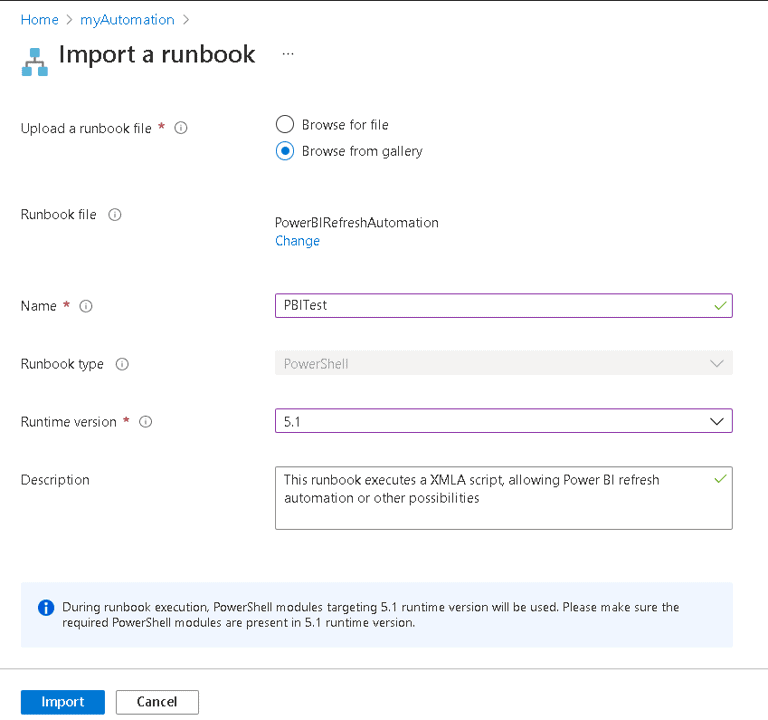
3) Click on the Select button. You will need to fill the details about the new runbook which will be created.


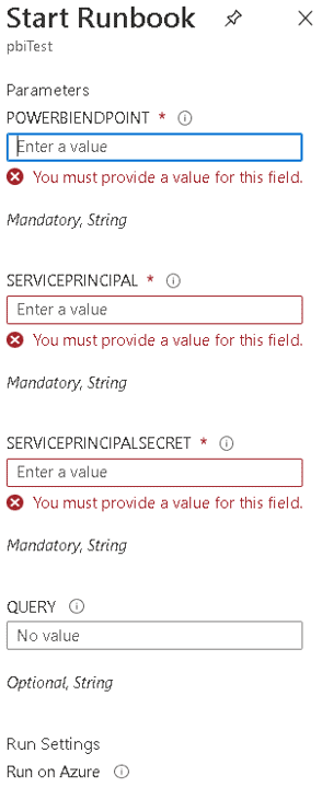
4) After clicking Import button, you can execute the runbook clicking the Start button and you will have the opportunity to fill the parameters for the powershell script, as illustrated on the screen below.


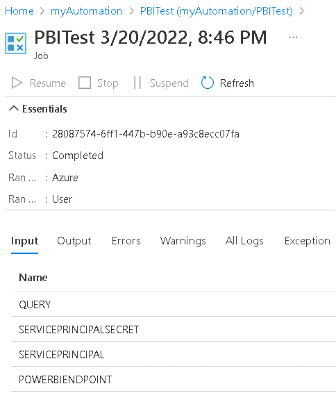
5) After that, you just need to follow the execution from the job screen.


Summary

Using the script provided in the automation gallery is even easier to automate a refresh or other administrative tasks in Power BI with XMLA scripts


The post Template for automating Power BI Refresh appeared first on Simple Talk.


from Simple Talk https://ift.tt/5K1sTDR
via