The Basics of Deleting Data from a SQL Server Table

Entry in Greg Larsen's series on Learning T-SQL. The series so far:

1. The basic T-SQL Select Statement
2. Ordering a result set in SQL Server
3. The ins and outs of joining tables in SQL Server
4. Summarizing data using GROUP BY and HAVING
5. The Basics of Inserting Data into a SQL Server Table
6. The Basics of Updating Data in a SQL Server Table

Over time data in SQL Server tables needs to be modified. There are two major different aspects of modifying data: updating and deleting. In my last article “Updating SQL Server Data” I discussed using the UPDATE statement to change data in existing rows of a SQL Server table. In this article I will be demonstrating how to use the DELETE statement to remove rows from a SQL Server Table.

Syntax of the Basic DELETE statement

Deleting data seems like a simple concept so you would think the syntax for a DELETE statement would be super simple. In some respects that is true, but there are many ways and aspects of how the DELETE statement can be used. In this article I will be discussing only the basic DELETE statement.

The syntax for basic DELETE statement can be found in Figure 1:

DELETE [ TOP (<expression>) [ PERCENT ] ] [ FROM ] <object> [ WHERE <search_condition>]

Figure 1: Basic syntax of the DELETE statement

Where:

• expression – Identifies the number or percentage of rows to be delete. When only the TOP keyword is identified the expression identifies the number of rows to be deleted. It the keyword PERCENT is also included then the expression identifies the percentage of rows to be delete.
• object – Identifies the table or view from which rows will be deleted.
• search_condition – Identifies the criteria for which a row must meet in order to be deleted. The search_condition is optional. When it is excluded from a DELETE statement, then all the rows in the object will be deleted.

For the complete syntax of the DELETE statement refer to the Microsoft Documentation which can be found here.

To better understand the syntax of the simple DELETE statement and how to use it, several examples are provided below. But before these examples can be run a couple sample tables need to be created.

Sample Data

Listing 1 contains a script to create two sample tables in the tempdb database.

USE tempdb;
GO

CREATE TABLE dbo.LoginTracking (
ID INT IDENTITY(1,1),
LoginName varchar(100),
LoginDataTime datetime,
LogoffDateTime datetime);
GO

INSERT INTO dbo.LoginTracking VALUES
('Scott','2022-07-11 08:41:31','2022-07-11 11:45:50'),
('Sally','2022-07-11 08:55:27','2022-07-11 11:59:59'),
('Dick','2022-07-11 09:05:17','2022-07-11 16:15:37'),
('Dick','2022-07-12 08:05:11','2022-07-12 15:50:31'),
('Scott','2022-07-12 08:12:27','2022-07-12 16:11:22'),
('Sally','2022-07-12 09:20:06','2022-07-12 16:45:11'),
('Dick','2022-07-13 08:10:13','2022-07-13 15:59:45'),
('Scott','2022-07-13 08:12:37','2022-07-13 16:21:38'),
('Sally','2022-07-13 09:07:05','2022-07-13 16:55:17');
GO

CREATE TABLE dbo.LoginsToRemove(
LoginName varchar(100));
GO

INSERT INTO dbo.LoginsToRemove VALUES ('Sally');
GO

Listing 1: Script to create sample tables.

The first table created in Listing 1 is the dbo.LoginTracking table. This table is the table from which rows will be deleted. The second table created is dbo.LoginsToRemoved. This table is a staging table that contains a single column named LoginName. This table will be used to show how to delete rows using rows in another table.

If you would like to follow along and run the code in this article you can use Listing 1 to create the two sample tables in the tempdb database on your instance of SQL Server.

Deleting a Single Row

To delete a single row, the DELETE command needs to identify the specific row that needs to be deleted. This is done by including a WHERE constraint. The WHERE constraint needs to uniquely identify the specific row to delete. The code in Listing 2 will delete the LoginTracking record that have a LoginName “Scott” and an ID value of 1.

USE tempDB;
GO

DELETE FROM dbo.LoginTracking
WHERE LoginName = 'Scott' and ID = 1;
GO

Listing 2: Deleting a single row

In the LoginTracking table there are multiple rows that have a LoginName of “Scott”. Therefore the ID column value of “1” was also included in the search_condition to uniquely identify which single row was to be deleted.

Only the ID column alone could have been used to identify the single record to be deleted. However, in many cases having extra filter conditions can be useful. For example, if the row where ID = 1 has a different LoginName, it would not be deleted.

Note: When you are expecting a certain number of rows to be deleted, it is a good idea to check the value in @@ROWCOUNT to make sure.

Deleting Multiple Rows

A single DELETE statement can also be used to delete multiple rows. To delete multiple rows the WHERE clause needs to identify each row in the table or view that needs to be deleted. The code in Listing 3 identifies two LoginTracking rows to delete by identifying the ID column values for the rows to be deleted.

USE tempDB;
GO

DELETE FROM dbo.LoginTracking
WHERE ID = 2 or ID=3;
GO

Listing 3: Deleting multiple rows with a single DELETE statement

By specify a WHERE clause, that identifies multiple rows the code in Listing 2 will delete multiple rows in the LoginTracking table when this code is executed.

Using the TOP Clause to Delete Rows of Data

When the TOP clause is included with a DELETE statemen, it identifies the number of random rows that will be deleted from the table or view being referenced. There are two different formats for using the TOP clause. (1) identifies the number of rows to be delete.

The code in Listing 4 shows how to use the TOP clause to delete one random row from the LoginTracking table.

USE tempdb;
GO

DELETE TOP(1) FROM dbo.LoginTracking; 
GO

Listing 4: Deleting one row using the TOP clause

The reason the top clause deletes random row is because SQL Server does not guarantee the order rows will be returned, without an ORDER clause.

If you need to delete rows in a specific order, it is best to use a subquery that uses TOP and an order by, as shown in Listing 5.

USE tempdb;
GO

DELETE TOP (2) FROM dbo.LoginTracking
WHERE ID IN 
   (SELECT TOP(2) ID FROM dbo.LoginTracking ORDER BY ID DESC);
GO

Listing 5: Deleting the last 2 rows based in ID

Executing the code in Listing 5 deletes the last two rows in the LoginTracking table, based on the descending order of the ID column. The code accomplished this by using a subquery in the WHERE constraint. The subquery uses the TOP clause to identify the two ID values that will be deleted based on descending sort order. This list of ID values is then used as the WHERE filter condition to identify the two rows to be delete.

Note: in this case, the TOP (2) in the DELETE is technically redundant. But if the ID column didn’t contain unique values, and the TOP clause would need to be included to make sure only two rows would have been deleted,.

The TOP clause in the prior two examples identified a specific number of rows to be deleted. The TOP clause also supports identifying a percentage of rows to delete. Before showing an example of deleting a percentage of rows using the TOP clause let’s first review the details of the rows still in the LoginTracking table, by running the code in the Listing 6.

USE tempdb;
GO

SELECT * FROM dbo.LoginTracking;

Listing 6: Displaying the rows currently in the dbo.LoginTracking table

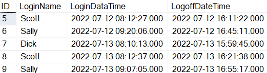
When the code in Listing 6 is run the results in Report 1 are displayed.

Report 1: Current rows in the LoginTracking table.

Currently there are 5 rows in the LoginTracking table.

To delete a percentage of the rows in a table the TOP clause is use along with the PERCENT keyword. The expression provided provide with the TOP clause identifies the percentage of rows to delete. The code in Listing 7 specifies 41 percent of the rows in the LoginTracking table should be deleted.

USE tempdb;
GO
DELETE TOP(41) PERCENT FROM dbo.LoginTracking;
GO
SELECT * FROM dbo.LoginTracking;
GO

Listing 7: Deleting 41 percent of the rows using the TOP clause.

When Listing 4 is executed the output in Report 2 is displayed.

Report 2: Number left in LoginTracking after the code in Listing 7 was run

By reviewing Report 2 and comparing it with Report 1 results, you can see 3 rows were deleted, which means 60 percent of the rows were deleted. Why 60 percent? The reason 60 percent of the rows were deleted is because SQL Server needs to delete a percentage of rows that equates to a whole number. Since 41 percent of 5 rows would have been 2.05 of the rows in the LoginTracking tracking table, SQL server rounded the row count up to 3. 3 equates to 60 percent of the rows when it performed the DELETE statement.

Using a Table to Identify the Row to Delete

There are times when you might need to identify rows to delete based on a table. To show how to delete rows based on rows in a table, the LoginsToRemove table was created in Listing 1. The LoginsToRemove table could be considered a staging table, which identifies the logins that need to be deleted. The code in Listing 8 uses this table to delete rows from the LoginTracking table.

USE tempdb;
GO

DELETE FROM dbo.LoginTracking
FROM dbo.LoginTracking JOIN dbo.LoginsToRemove
ON LoginTracking.LoginName = LoginsToRemove.LoginName
GO

Listing 8: Using a table to identify rows to be deleted from a table

The code in Listing 8 joined the LoginsToRemove table with the LoginTracking table on the LoginName column from each table. This join operation only finds those rows in the LoginTracking table which have a matching LoginName in the LoginsToRemove table. In this example all the records that had “Sally” as a LoginName got deleted from the LoginTracking table.

Deleting all Rows from a Table

The DELETE statement can be used to remove all the rows in a table. To accomplish this a DELETE Statement without a WHERE constraint can be executed, as in Listing 9.

USE tempdb;
GO

DELETE FROM dbo.LoginTracking;
GO

Listing 9: Deleting all the rows in a table.

Even though the DELETE statement can delete all the rows in a table, as done in Listing 9, this is not the most efficient way to delete all the rows in a table. The DELETE statement performs a row-by-row operation to delete all the rows. Every time a row is deleted information needs to be written to the transaction log file, based on the database recovery model option. If there are a lot of rows in a table, it could take a long time and use a lot of resources to delete all the rows using a DELETE operation.

An alternative method to remove all rows in a table

A more efficient, though more limited method to delete all rows is to use the TRUNCATE TABLE statement as shown in Listing 10.

USE tempDB;
GO

TRUNCATE TABLE dbo.LoginTracking;
GO

Listing 10: Deleting all the rows in a table using a TRUNCATE TABLE statement

When a TRUNCATE TABLE statement is used, less information is logged to the transaction log file, as well as has some other significate differences. One of those differences is when a DELETE statement is used, if all the rows are deleted from a physical DATA page the page is left empty in the database, which wastes valuable disk space. Additionally, a TRUNCATE TABLE option requires less locks to remove all the rows.

Another important difference is how these two different delete methods affect the identity column’s seed value. When a TRUNCATE TABLE statement is executed the seed value for the identity column is set back to the seed value of the table. Whereas the DELETE statement retains the last identity column value inserted. This means when a new row is inserted, after all the rows were deleted, using a DELETE statement, that the next identify value will not start at the seed value for the table. Instead, the new row’s identity value will be the determined based off the last identity value inserted, and the increment value for the identity column. These differences need to be kept in mind when deleting rows using the DELETE statement during testing cycles.

There are two major limitations to consider. First, the table being truncated cannot be referenced in a FOREIGN KEY constraint. The second is security. To be able to execute a DELETE statement that references a table, you need DELETE permissions. To execute TRUNCATE TABLE you need ALTER TABLE rights, which gives the user the ability to change the table’s structure. For more details on TRUNCATE TABLE, check the Microsoft documentation here.

Deleting data using a view

Deleting from a view is the same as deleting from a table, with one caveat. The delete can only affect one table. This essentially means that the FROM clause of the view can only reference one table to be the target of a DELETE statement. You could have conditions (like subqueries) that reference other objects, but no joins. For example, in listing 11, consider the two view objects.

CREATE VIEW dbo.v_LoginTracking
AS
SELECT ID,
       LoginName,
       LoginDataTime,
       LogoffDateTime
FROM   dbo.LoginTracking;
GO

CREATE VIEW dbo.v_LoginTracking2
AS
SELECT LoginTracking.ID,
       LoginTracking.LoginName,
       LoginTracking.LoginDataTime,
       LoginTracking.LogoffDateTime
FROM dbo.LoginTracking JOIN dbo.LoginsToRemove
ON LoginTracking.LoginName = LoginsToRemove.LoginName
GO

Listing 11: View objects to demonstrate how deleting from a view works

Executing a DELETE statement in the first view: dbo.v_LoginTracking, will work. But attempt to delete rows using the second view: dbo.v_LoginTracking, and you will get the following error.

View or function 'dbo.v_LoginTracking2' is not updatable because the modification affects multiple base tables.

Deleting Rows from a SQL Server table

The DELETE statement is used to delete rows in a SQL Server table or view. By using the DELETE statement, you can delete one or more rows from an object. If all the rows in a table need to be deleted, a DELETE statement is less efficient then using the TRUNCATE TABLE statement, but has fewer limitations and doesn’t reset the identity value information.

Knowing how to use the basic DELETE statement, and when not to use it is important concept for every TSQL programmer to understand.

 

The post The Basics of Deleting Data from a SQL Server Table appeared first on Simple Talk.

from Simple Talk https://ift.tt/sq5zk1R
via

How to Use Any SQL Database in GO with GORM

Object Relational Mapping is a database abstraction technique that aids developers in manipulating and interacting with SQL databases using the data types provided in the programming language.

ORMs (Object Relational Mappers) are tools (libraries, modules, packages) that provide the functionality for interacting with SQL databases. Popular ORMs are the Prisma ORM for JavaScript, TypeScript, Hibernate for Java, and SQLAlchemy for Python.

Aside from the benefit of interacting with SQL databases in a more natural manner than writing raw SQL, there are many other benefits of using ORMs. Without worrying too much about compatibility, you can use any databases supported by an ORM with the same code (when using common functionality, not every feature will be available for every database type.)

GORM is the most popular ORM in the Go ecosystem. GORM (Go-ORM) is a developer-friendly, full-featured, Code-first ORM for interacting with SQL databases in Go. GORM provides drivers and functionalities like associations, automigration, SQL building, logging, and hooks for database operations, and support for popular SQL databases including MySQL, SQLite, PostgreSQL, Microsoft SQL server, and many database drivers.

Getting Started with GORM

You’ll need to meet a few requirements to get the most out of this article.

• You have experience working with Go and have Go installed on your machine.
• You have experience working with SQL and SQL databases.

In this tutorial, you’ll learn how to use GORM with an SQLite database. The processes are generally the same for all other supported SQL databases.

After creating a Go workspace, Install the GORM package using these commands in your working directory.

go get gorm.io/gorm

You’ll need a database driver to work with GORM. Fortunately, GORM also provides database drivers for the popular SQL databases. Install the database driver for your preferred database using any of these commands.

go get gorm.io/driver/sqlite //SQLite 
go get gorm.io/driver/mysql // MySQL 
go get gorm.io/driver/postgres //PostgreSQL 
go get gorm.io/driver/sqlserver //MSSQL 
go get gorm.io/driver/clickhouse //click house

GORM also provides functionalities for using custom database drivers. This is beyond the scope of this article, but you can read more here.

After installing your database driver, you can import the driver for use.

import ( 
        "gorm.io/gorm" 
        _ "github.com/mattn/go-sqlite3" 
      )

As shown above, you’ll have to import the database driver for side effects. (This allows interactions with the database over GORMs interface to do things like query and modify data.)

Connecting to Databases using GORM

After installing and importing the GORM package and your preferred database driver, you can proceed to connect to your database.

Use the Open method of the gorm module to connect to a database. The Open method takes in the connection and configuration methods as input and returns the database connection instance.

db, err = gorm.Open(sqlite.Open("Blogs.db"), &gorm.Config{})
 
if err != nil { 
     panic("failed to connect database") 
}

The previous code connects to an in-memory SQLite database in the code example above. For SQLite, the Open method creates a database in your working directory if the database doesn’t exist. The process is similar if you connect to a database with a connection string. In the following code, I am connecting to a MySQL database using a connection string.

Db, err =        gorm.Open(mysql.Open(“root:admin@tcp(127.0.0.1:3306)/yourdatabase?charset=utf8mb4&parseTime=True&loc=Local”), &gorm.Config{}) 
if err != nil { 
   panic(“failed to connect database”) 
}

Connecting to a database is similar if you use a custom database driver. You must connect to the database based on the specifications that were included in the driver, and pass the connection details to the Open method.

Db, err := gorm.Open(“sqlite3”, “./app.db”)

In this case, you’re using the custom SQLite driver imported above. On a successful database connection, you’ll be able to interact with the database with Go data types in the same way.

Mapping Go Types With GORM

GORM is a code-first ORM. This means you won’t have to define your schema in SQL. For GORM, you use Go structs to describe the schema and column types with GORM tags.

Type Human struct { 
   Age int 
   Name string 
}

On migration, the Human struct will be translated to the database schema. The table’s name in the database will be Human and the Age and Name fields are the column names.

GORM provides tags for adding SQL constraints like primary key, foreign keys, index, not null and other database constraints. Here’s how you can add a GORM tag to a struct.

type Human struct { 
    Age int `gorm:"primaryKey"` 
    Name string `gorm:"size:255;not null;unique"` 
}

The Age field has a primary key constraint, and the Name field has size, not null and unique constraints.

For easy schema modelling, GORM provides the GORM Model. The GORM model is a struct that contains popularly used fields like ID as the primary key and the created, updated, and deleted time as columns. You can use the Model struct by passing the model to your struct.

type Human struct { 
   gorm.Model 
   Age int `gorm:"primaryKey"` 
   Name string `gorm:"size:255;not null;unique"` 
}

The Human struct above evaluates to the HumanPlus struct below in the database on migration since the Human struct inherits the gorm.Model struct.

type HumanPlus struct { 
   Age int `gorm:"primaryKey"` 
   Name string `gorm:"size:255;not null;unique"` 
   ID uint `gorm:"primaryKey"` 
   CreatedAt time.Time 
   UpdatedAt time.Time 
   DeletedAt gorm.DeletedAt `gorm:"index"` 
}

You can embed your custom structs in other structs using the embedded tag.

type Human struct { 
   Age int `gorm:"primaryKey"` 
   Name string `gorm:"size:255;not null;unique"` 
} 
type Beings struct { 
   human Human `gorm:"embedded"` 
   gorm.Model 
}

The Beings struct eventually evaluates to the Evaluate struct below on migration.

type Evaluate struct { 
   Age int `gorm:"primaryKey"` 
   Name string `gorm:"size:255;not null;unique"` 
   ID uint `gorm:"primaryKey"` 
   CreatedAt time.Time 
   UpdatedAt time.Time 
   DeletedAt gorm.DeletedAt `gorm:"index"` 
}

GORM supports most features you’ll want in an ORM, including functionality to set field permissions for more data control. Here’s the complete reference from the GORM documentation.

type User struct { 
   Name string `gorm:"<-:create"` // allow read and create 
   Name string `gorm:"<-:update"` // allow read and update 
   Name string `gorm:"<-"` // allow read and write (create and update) 
   Name string `gorm:"<-:false"` // allow read, disable write permission 
   Name string `gorm:"->"` // readonly (disable write permission 
                           //unless it       configured) 
   Name string `gorm:"->;<-:create"` // allow read and create 
   Name string `gorm:"->:false;<-:create"` // create only (disabled read 
                                                          //from db) 
   Name string `gorm:"-"` // ignore this field when writing and 
                          //reading with struct 
   Name string `gorm:"-:all"` // ignore this field when writing, 
                              //reading and migrating with struct 
   Name string `gorm:"-:migration"` // ignore this field when migrate 
                                    //with struct 
}

Setting up Automigrations With GORM

Automigrations are one of the significant benefits of using ORMs, making it easy to add data entries. You can migrate instances of the struct model using the AutoMigrate method of the database instance.

err = db.AutoMigrate(&Human{}) 
if err != nil { 
    panic("migration failure") 
}

By referencing the struct here, you’ve set the Human struct for auto migration. The AutoMigrate method returns an error that you can handle if any.

Conventionally, you’ll use the function that returns your database instance to set up auto migrations and return the database instance.

func database(DNS string) *gorm.DB { 
   var db *gorm.DB 
   db, err = gorm.Open(mysql.Open(DNS), &gorm.Config{}) 
   if err != nil { 
      panic("failed to connect database") 
   } 
   err = db.AutoMigrate(&Human{}) 
   if err != nil { 
      return 
   } 
      return db 
   }

Inserting Into a Database With GORM

The Create method accepts a reference to the struct initialization and inserts a new row to the database.

person := Human{ 
   Model: gorm.Model{}, 
   Age: 18, 
   Name: "James Dough", 
} 
db.Create(&person)

Depending on your operation; you can use many methods and functions on the Create method.

Using the RowsAffected method on the Create method returns the number of Rows affected.

rows := db.Create(&person).RowsAffected 
log.Println(rows)

There are many other methods you can use with the Create method. In figure1 you can see a few of them.

Figure 1 – Additional methods you can use with the Create method.

Reading From a Database With GORM

Reading from a database with GORM is easy, and there are many methods you can use based on the operation.

The read methods decode the query result into an instantiated struct.

type person := new(Human)

The Take , First , and Last methods return a single row. The Take method returns a random row that meets the criteria; the First method returns the first entry that satisfies the query ordered primary key, and the Last method returns the last entry that satisfies the query ordered primary key.

db.Take(&person, "John") 
db.First(&person, "Jane") 
db.Last(&person, "Dough")

Using the Find method, you can also query for all the rows that meet the criteria.

db.Find(&person, "James")

You can use the Where method with any of the Find , First , Take and Last methods for complex queries.

db.Where("Name = ? AND Age >= ?", "James", "22").Find(&person)

Updating Database Entries With GORM

Update operations are easy and quite similar to other GORM operations, and all the methods and functions on read operations are also available.

You can update a column using the Update method after referencing the struct table you want to update using the Model method.

var rows = db.Model(&Human{}).Update("Name", "Junior").RowsAffected

After a successful update operation, the rows variable will store the number of rows affected by the operation.

You can also update multiple columns using the Updates method. The Updates method takes in an initialized struct.

person := Human{ 
    Name: "James", 
    Age: 18, 
} 
db.Model(&person).Updates(person)

Like the read operation, you can use the Where method with any update methods for complex operations.

db.Model(&Human{}).Where("Age = ?", 19).Update("Name", "Junior")

Deleting From a Database With GORM

You can use the Delete method to delete rows in a database. The Delete method takes in the instantiated struct type.

db.Delete(&person)

You can also use the Delete method on the Where method for complex operations

db.Where("name = ?", "John").Delete(&person)

If you need to delete specific columns, You can drop a column using the DropColumn method of the Migrator method of the database instance.

err := db.Migrator().DropColumn(&Human{}, "Name") 
if err != nil { 
return 
}

Here you dropped the Name column of the Human table. The DropColumn method returns an error if there’s any.

The GORM SQL Builder

One of the cons of using ORMs, in general, is the abstraction ORMs provide over the database, reducing the power and flexibility of interacting with databases. Most ORMs like GORM provide SQL builders for raw SQL queries and operations.

You can use the Raw method to write raw SQL queries. The methods on the Raw method serve various functionalities. The Scan method returns the result of the query into the instantiated struct.

type Result struct { 
   ID int 
   Name string 
   Age int 
}
 
var output Result 
db.Raw("SELECT id, Name, Age FROM Human WHERE Name = ?", "James").Scan(&output)

In this case, GORM would decode the output of the SQL query into the output variable You can also execute SQL statements using the Exec method of your database instance.

db.Exec("DROP TABLE Human")

Conclusion

GORM provides most of the functionalities you’ll need in an ORM while prioritizing efficiency and security, making the library every Go developer’s choice for interacting with SQL databases.

In this tutorial, you learned about the GORM library to increase productivity while interacting with databases with Go. You can perform many more operations with the GORM library, and this article has given you an overview. You can check out GORM’s documentation to learn more about the library.

 

The post How to Use Any SQL Database in GO with GORM appeared first on Simple Talk.

from Simple Talk https://ift.tt/TliFZgu
via

Calling all leaders: People matter

At the turn of the millennium, I was a young adult, just finished education and starting my very first job at a software company. I was excited, enthusiastic, and felt well-prepared for a life of “Office 9 to 5” and was looking forward to earning my keep. But I was naïve when it came to understanding how people work together in an organization. Here was no distinguished professor to teach lessons, no defined curriculum to structure lessons around, and no predictability about what those lessons might even be. There were unwritten rules, underlying currents, politics, and stratagems aplenty. In an office surrounded by thousands of colleagues, I was still on my own.

Twenty or so years later, I am happy to say that I have kept most of my energy and enthusiasm, while also learning a thing or two about how corporate culture works. I have learned many lessons: Communication is important. Context is key. Expertise earns respect. Boldness, curiosity, and experimentation can be admirable yet intimidating. But my biggest lessons have been that everyone works differently and people’s feelings matter. Nothing highlights this better than the contrast between two different companies I went on to work with. Both were small companies with less than 30 employees. Both were family-owned and run. Both were in the same geographic area and both benefited from the same economic advantages.

Company A treated its employees poorly. We were ordered to follow instructions and discouraged from challenging anything. “Write this document” meant the document had to be written, regardless of whether it was necessary or not, whether anyone would read it or not, or whether there was a better way to do something or not. Senior managers were never present to hear from us: they declined meeting requests, gave brief answers to text messages, and often went off on a tangent when asked for clarification about any topic. We were expected to work far beyond the hours we were paid for, and to be at our desk at 08:30 and still be there until 18:30. There were other things: micromanagement was off the scale, all communication had to take place by email to “maintain records” because there was a culture of finger pointing and blame shifting, customer complaints were ignored, timesheets had to be documented to the minute, and getting appreciated for good work was like drawing blood from stone.

I lasted six months before I got out.

Company B was an employee haven. We were treated with respect. Our views were sought, heard, and frequently followed. We were encouraged to have interests outside of our work area of expertise, to explore, and to self-develop. Senior managers were always available to listen to our problems and help us find our own solutions. We had regular team events, Friday evening drinks, and even a small bonus at Christmas. Company meetings always highlighted team achievements and celebrated our successes. Managers were flexible with work timings, and we willingly volunteered to cover for each other should someone need to leave office during work hours.

I stayed two years and would probably never have left had I not moved to another country.

The first company’s leadership made my colleagues and me feel frustrated, mistrustful, and self-serving. The result was that there was never a spirit of team or community.

The second company’s leadership made us feel valued and respected. The result was that we worked as a team and did our best to meet our customers’ expectations, to delight them and grow the company’s business.

Company A has now gone bust. Company B has grown into a multi-subsidiary group with headquarters in a major European capital city and branches in other locations.

It is people who make the organization. Even history has many examples, from dictators to presidents, some of the unlikeliest folk to have become leaders. Yet, they did.

I believe people follow people, not intangible “ideals.”

 

The post Calling all leaders: People matter appeared first on Simple Talk.

from Simple Talk https://ift.tt/g5JwTuX
via

The PASS Sessions I Am Most Excited For

The PASS Data Community Summit is coming up in less than three weeks, so it is time to start finalizing your schedule. My schedule this year is fixed, as I will be working behind the scenes helping to manage one of the live online tracks. But that doesn’t stop me from checking the sessions I will be making sure I watch after the show is over if I don’t see them live.

Note: The sessions mentioned are based on things that Louis Davidson (me!) is interested in and doesn’t say anything about sessions I am not mentioning. While I now edit the Simple-Talk website, I will continue to be a data architect/programmer at heart. Hence my preferred sessions are going to be heavily T-SQL programming centric when I am choosing for me.

While I am Producing

Just looking at the list of sessions I am pretty sure I will be involved with, there are some sessions that I want to see either way. For example:

Note: you will need to register/login to follow these links. If you haven’t registered, time is running out! Go to PASS Data Community Summit and register.

In-Memory OLTP Design Principles by Tosten Strauss. I have been fascinated by the memory-optimized objects in SQL Server for many years, though I haven’t used the feature even in a demo manner for a while. I have built quite a bit of sample code with it, but always love to hear more.

SQL Server Table Partitioning – DOs and DON’Ts by Margarita Naumova. Partitioning is not something I have ever done in a production setting, and it is really one of the features in SQL Server that I have never even written very much demo code on. As such it is a topic I always wanted to know more about for that day when I need to implement it (or tech edit a blog about it!).

SSIS Custom Pipeline Component: A Step-by-Step Guide by Arne Bartels. I have spent a lot of time over the past 15 years building SSIS Packages, and I will probably continue to build them to more data around in my personal projects as well.

While I may not professionally build SSIS packages now (and maybe not ever), sometimes it is fun to go to a session and learn all the things you could have done better.

---

Does this mean I won’t enjoy An Introduction to S3 Data Lake for SQL Server 2022 by Chris Adkin, Getting started with Power BI Deployment Pipelines by Akshata Revankar., Better Data Governance with Purview by Kelly Broekstra, or any of the other sessions I will be in? If you think that, you may have skipped the introduction to this blog. Clearly the answer is “no”. In fact, since I will just be where I am told, I have only barely looked at the schedule after it posted. The sessions may have had a time change since last I looked.

The three highlighted sessions are ones I would have in my list to stream after the conference anyhow!

Saving for Later

I have scanned the schedule a few times and have quite a few more sessions that would be not-miss, front row attenders if I was in Seattle. Of course, the reality is that even if I was there in-person, I still probably would have missed a few. Sometimes it is because there are two sessions that overlap each other (the committee tries to not let that happen for sessions that suit a certain persona (like database programmer), but there are only so many slots to hold sessions. The far more common reason I tend to miss sessions is that I know at least 100-300 people that will be at the Summit… that’s a lot of catching up to do (especially since I haven’t been to a conference in almost three years)!

There are plenty of sessions I will do my best to watch after the week is over. It is aways a bit difficult to find the time to go back and watch every session you want to, but there are a few sessions that I expect really need to be attended.

First and foremost, any session by Itzik Ben-Gan is going on my list, and I love the topic of the Beware Nondeterministic T-SQL Code section too. Honestly, I might know everything he is going to say in this presentation, but Itzik digs deep enough that there are usually an Aha Moment or twenty..

Really though, even sessions where you think you are an expert there is almost always the possibility of learning something new. Just last night, I reviewed a potential writer’s article on a subject I know quite well, but I still learned a few things! On the other hand, in Itzik’s case, it is possible that I might end up having no idea what he is talking about until I watch it a few times, so watching the recording won’t be all bad.

How to Maintain the Same Level of utilities in Cloud Deployments by Denny Cherry

As we all move to the cloud, even those of us who just write about SQL Server for the most part, this question is big in our minds. “How do I use the skills I have in the new world?” Plus, Denny is an entertaining speaker no matter what!

A Query Tuner’s Practical Guide to Statistics by Andy Yun.

Statistics are kind of a mystery to most people, even somewhat me at times. For the most part, we ignore them and let the engine do its thing. But sometimes… well a query is slow. Looking at the query plan, you see guesses about how many rows need to be processed and the actual number of rows processed is orders of magnitude greater. The common blame? Statistics.

Take knowledge that is useful and add to that the fact that Andy is a great speaker, and this one seems like a lock.

And so on

I could go on. I looked at the schedule quite a few times as part of the committee to choose sessions (I helped validate the sessions and schedules before starting here at Redgate) and there are so many great sessions no one could see them all, or even sit down and pick just a few to highlight. I didn’t even mention Paul Randal’s Performance Mythbusters session, Glenn Berry’s Index Tuning 101, Intelligent Data through Data Intelligence by Chris Unwin, SQL Titbits for the Inexperienced by Erland Sommarskog…any of the keynotes, precons, or so many others.

All this and these are just a handful (maybe two handfuls) of sessions that fit what I like best/ There are like 300 sessions plus to choose from all over the variety of topics the data platform provides.

See you soon!

 

The post The PASS Sessions I Am Most Excited For appeared first on Simple Talk.

from Simple Talk https://ift.tt/OjUQBlR
via

Introducing the MySQL UPDATE statement

Entry in Robert Sheldon's series on Learning MySQL. The series so far:

1. Getting started with MySQL
2. Working with MySQL tables
3. Working with MySQL views
4. Working with MySQL stored procedures
5. Working with MySQL stored functions
6. Introducing the MySQL SELECT statement
7. Introducing the MySQL INSERT statement

The UPDATE statement enables you to modify values in your database tables, including temporary tables. With a single statement, you can update one or more rows, one or more columns, or any combination of the two. You can even update multiple tables. As you work through this article, you’ll find that the UPDATE statement is intuitive and straightforward to use, once you understand the basics of how it works.

Preparing your MySQL environment

For the examples in this article, I used the same database (travel) and tables (manufacturers and airplanes) that I used for the last few articles in this series.

Note: The examples assume that you worked through the previous article, in which case, the travel database should be set up and ready to go. If you did not, you can still follow along with this article, just know that your query results will be slightly different from the ones I show here.

To set up the travel database—if you haven’t already done so—download the MySQL_06_setup.sql file and run the SQL script against your MySQL instance. The script creates the database and tables and inserts sample data. Alternatively, you can create the database and then run the following script to create the manufacturers and airplanes tables:

CREATE TABLE manufacturers (
  manufacturer_id INT UNSIGNED NOT NULL AUTO_INCREMENT,
  manufacturer VARCHAR(50) NOT NULL,
  create_date TIMESTAMP NOT NULL DEFAULT CURRENT_TIMESTAMP,
  last_update TIMESTAMP NOT NULL 
    DEFAULT CURRENT_TIMESTAMP ON UPDATE CURRENT_TIMESTAMP,
  PRIMARY KEY (manufacturer_id) ) 
ENGINE=InnoDB AUTO_INCREMENT=1001;

CREATE TABLE airplanes (
  plane_id INT UNSIGNED NOT NULL AUTO_INCREMENT,
  plane VARCHAR(50) NOT NULL,
  manufacturer_id INT UNSIGNED NOT NULL,
  engine_type VARCHAR(50) NOT NULL,
  engine_count TINYINT NOT NULL,
  max_weight MEDIUMINT UNSIGNED NOT NULL,
  wingspan DECIMAL(5,2) NOT NULL,
  plane_length DECIMAL(5,2) NOT NULL,
  parking_area INT GENERATED ALWAYS 
             AS ((wingspan * plane_length)) STORED,
  icao_code CHAR(4) NOT NULL,
  create_date TIMESTAMP NOT NULL 
             DEFAULT CURRENT_TIMESTAMP,
  last_update TIMESTAMP NOT NULL 
    DEFAULT CURRENT_TIMESTAMP 
           ON UPDATE CURRENT_TIMESTAMP,
  PRIMARY KEY (plane_id),
  CONSTRAINT fk_manufacturer_id 
    FOREIGN KEY (manufacturer_id) 
       REFERENCES manufacturers (manufacturer_id) ) 
ENGINE=InnoDB AUTO_INCREMENT=101;

Next, you need to add data to the manufacturers and airplanes tables to support the examples in this article. Start with the manufacturers table by running the following INSERT statement, which adds Beagle Aircraft Limited as a manufacturer:

INSERT INTO manufacturers (manufacturer)
VALUES ('Beagle Aircraft Limited');

SELECT manufacturer_id
FROM   manufacturers
WHERE  manufacturer = 'Beagle Aircraft Limited';

After the data is inserted, the SELECT statement returns the newly added value from the manufacturer_id column. If you’ve been following along exactly with the last couple of articles, the value would be 1008. If it is not, make a note of the manufacturer_id value you get here because you’ll need it for the rest of the article, starting with the following INSERT statement:

INSERT INTO airplanes 
  (plane, manufacturer_id, engine_type, engine_count, 
    wingspan, plane_length, max_weight, icao_code)
VALUES 
  ('A.61 Terrier',1008,'piston',1,36,23.25,2400,'AUS6'),
  ('B.121 Pup',1008,'piston',1,31,23.17,1600,'PUP'),
  ('B.206',1008,'piston',2,55,33.67,7500,'BASS'),
  ('D.4-108',1008,'piston',1,36,23.33,1900,'D4'),
  ('D.5-108 Husky',1008,'piston',1,36,23.17,2400,'D5');

If necessary, replace 1008 with your manufacturer_id value and then run this statement. After you’ve done that, you should be set up to follow along with the examples in this article. Be aware, however, that a number of the following examples reference the manufacturer_id column, so if the value is not 1008 on your system, be sure to use the correct one.

The UPDATE statement syntax

The UPDATE statement in MySQL supports five clauses, two of which are required and three that are optional, as indicated in the following syntax:

UPDATE [IGNORE] table_name
SET column = value [, column = value]...
[WHERE where_condition]
[ORDER BY order_list]
[LIMIT row_count]

The syntax does not include all the elements in an UPDATE statement, but it does provide most of them. These are ones you’ll be using the majority of the time, not only when learning about the statement, but also after you’ve mastered it. For the complete syntax check the MySQL documentation on the UPDATE statement.

Here’s a breakdown of the five clauses:

• The UPDATE clause, one of the statement’s two mandatory clauses, specifies the table that is the target of the update. You can specify multiple tables in this clause, separating them with commas, but my focus in this article is on single-table updates. I’m saving the subject of multi-table updates for when I cover more advanced topics.
• The SET clause, the other mandatory clause, specifies which columns to update. You can include one or more column assignments. For each assignment, specify the column name, an equal sign, and the new value. If you include multiple assignments, separate them with commas.
• The WHERE clause determines which rows to update, based on one or more conditions. The clause works much like the WHERE clause in a SELECT statement. Although the WHERE clause is optional, you should be very careful running an UPDATE statement that that does not include one. Without a WHERE clause, the statement will update every row in the table, unless the LIMIT clause is included.
• The ORDER BY clause specifies the order that rows should be updated. This can be useful in situations that might otherwise result in an error, as you’ll see later in the article. The ORDER BY clause is similar to the one you saw in the SELECT statement. The clause cannot be used for multi-table updates.
• The LIMIT clause limits the number of rows that will be updated. If you include a WHERE clause, the count applies to the rows returned by that clause. This means that the statement will stop based on the number of rows that satisfy the WHERE conditions, whether or not those rows are actually updated. As with the ORDER BY clause, the LIMIT clause cannot be used for multi-table updates.

With these five clauses, you can build a wide range of UPDATE statements. Most of the time, you’ll be using the UPDATE, SET and WHERE clauses, although the ORDER BY clause and LIMIT clause can also come in handy at times.

Once you see the statement in action, you should have no problem understanding how all the clauses work and using them to update data. In fact, it’s almost too easy to update data, and if you’re not careful, you could make a significant mess of things. Data modifications can be difficult to undo, so you need to proceed cautiously, especially when you’re first learning how to use the UPDATE statement. Certainly, don’t practice in a production environment. When you do update the production environment, be sure to do it within a transaction, a topic I plan to cover later in the series.

Performing a basic update in MySQL

Now that you have a basic overview of the UPDATE statement syntax, it’s time to see the statement in action so you can get a feel for how it works. As I already mentioned, the UPDATE and SET clauses are the only required clauses, so let’s start with them.

Suppose you want to round all the values in the wingspan column in the airplanes table to whole numbers. To achieve this, you create the following UPDATE statement:

UPDATE airplanes
SET wingspan = ROUND(wingspan);

The UPDATE clause identifies airplanes as the target table, and the SET clause specifies that the values in the wingspan column should be rounded, which is achieved by using the built-in ROUND function.

That’s all it takes to update the wingspan data. However, there’s a good chance that when you try to run this statement, you’ll receive the following error:

Error Code: 1175. You are using safe update mode and you tried to update a table without a WHERE that uses a KEY column. To disable safe mode, toggle the option in Preferences -> SQL Editor and reconnect.

By default, you cannot perform an update without a WHERE clause that specifies a key column. This helps to ensure that you don’t make sweeping changes that you’ll later regret. You can disable safe mode (as the error message suggests), either permanently or temporarily. I recommend that you do it on a temporary basis to avoid any unwanted changes elsewhere.

To temporarily disable safe mode, use a SET statement to change the SQL_SAFE_UPDATES system variable to 0 prior to running your UPDATE statement and then set the variable to 1 after you run the statement, as shown in the following example:

SET SQL_SAFE_UPDATES = 0;

UPDATE airplanes
SET wingspan = ROUND(wingspan);

SET SQL_SAFE_UPDATES = 1;

The SET statements merely toggle the variable off and then on during the current session. Be aware, however, that the SET statement supports the GLOBAL option, which sets a variable at the global scope. As a general practice, do not use this option when disabling safe updates. It is much less risky to make these sorts of changes at the session level to prevent any unplanned mishaps. Use GLOBAL only if it’s essential in your circumstances.

For more details on SET and global variables and settings. See Using System Variables in the MySQL Documentation.

Even at the session level, the SET statement makes it possible to execute your UPDATE statement without generating an error. You can confirm the changes by running a simple SELECT statement after executing the script above:

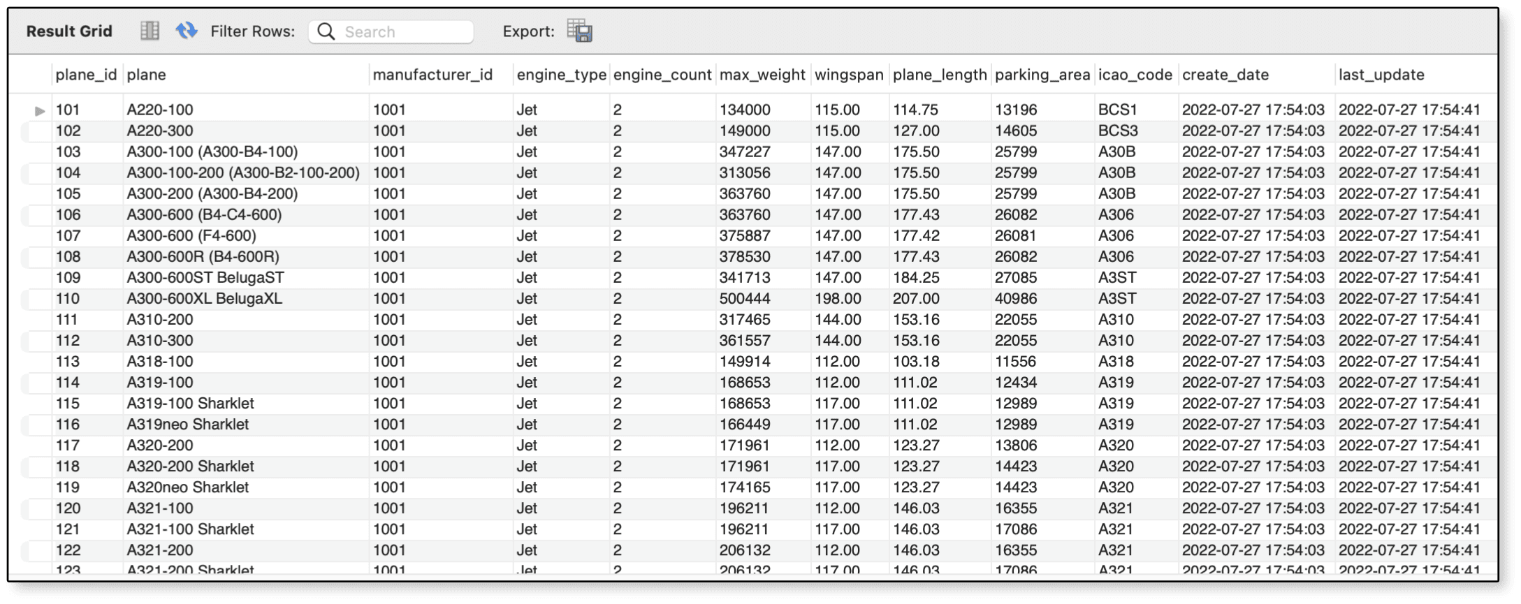
SELECT * FROM airplanes;

Figure 1 shows part of the results returned by the SELECT statement. Notice that the wingspan values are now all whole numbers.

Figure 1. Rounding the values in the wingspan column

In some cases, you might want to update multiple columns at the same time. For this, you need to add the additional column assignments, separating them with commas. For example, the following UPDATE statement modifies both the wingspan and plane_length columns:

SET SQL_SAFE_UPDATES = 0;

UPDATE airplanes
SET wingspan = ROUND(wingspan), plane_length = ROUND(plane_length);

SET SQL_SAFE_UPDATES = 1;

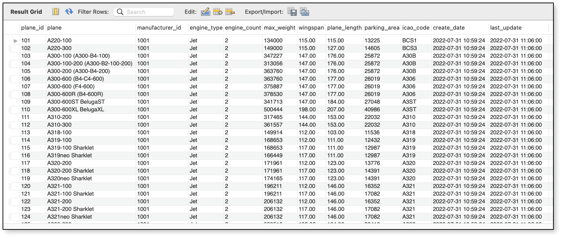
Both column assignments work the same way. You’re simply rounding the column values to whole numbers. If you were to query the airplanes table after running the UPDATE statement, your results would look similar to those shown in Figure 2.

Figure 2. Rounding the values in the wingspan and plane_length columns

By using the UPDATE and SET clauses, you can quickly update all of a column’s values. Just be careful if taking this approach. It’s all too easy to mess things up in a big way.

Adding a WHERE clause to your UPDATE statement

Most of your UPDATE statements will likely include a WHERE clause to help you better target the data that you want to modify. The WHERE clause specifies one or more conditions that narrow down the rows to be updated. For example, the following statement includes a WHERE clause that limits the updates to rows with a manufacturer_id value of 1008:

UPDATE airplanes
SET engine_type = 'piston (adg-i)' 
WHERE manufacturer_id = 1008;

SELECT *
FROM   airplanes
WHERE manufacturer_id = 1008;

The SET clause in this statement sets the engine_type value to piston (adg-i) for the targeted rows. The results from executing the statements should look similar to Figure 3.

Figure 3. Limiting your update to specific rows

Note: In case you’re wondering, the adg-i value is a reference to Airplane Design Group (ADG) classifications, a system used to categorize aircraft by dividing them into six groups based on their wingspans and tail heights. The lowercase i indicates that the planes in this example are in Group I. (I realize that you’d probably want to add a column for the ADG groups. The approach I took here was meant only to demonstrate these concepts.)

That said, it turns out that the B.206 airplane should actually be in Group II, which means you need to update that record without updating the others. Fortunately, you can define multiple conditions in your WHERE clause to help narrow down the rows. In the following example, the WHERE clause includes two conditions, one based on the manufacturer_id column and the other on the plane column:

UPDATE airplanes
SET engine_type = 'piston (adg-ii)'
WHERE manufacturer_id = 1008 AND plane = 'B.206';

As in the previous example, the WHERE clause limits the updates to rows with a manufacturer_id value of 1008. However, the clause also specifies that the plane value must equal B.206. The two conditions are linked together by the AND logical operator, which means that both conditions must evaluate to true for the row to be updated.

After you run the UPDATE statement, you can retrieve the same rows as before. Your results should look similar to those shown in Figure 4. Notice that the B.206 aircraft is now shown as a Group II plane.

Figure 4. Limiting your update to one specific row

You can make your WHERE clause as detailed as necessary to ensure that you’re updating the target rows and no other rows. The key is to use your logical operators correctly to ensure that your conditional logic is accurate.

Working with column values

In the first example in this article, you saw how to use the ROUND system function to round values in the airplanes table. When you update a column in this way, MySQL uses the column’s current value to create a new value. The ability to use the current value makes it possible to build on that value in ways that go beyond simply applying a function. For example, the following UPDATE statement adds 3 to the wingspan value and 5 to the plane_length value:

UUPDATE airplanes 
SET wingspan = wingspan + 3, plane_length = plane_length + 5 
WHERE plane_id = 344;

In this case, I used the plane_id value 344 in the WHERE clause, which I had to look up in the table. However, you might want to use a different method for finding this value, such as retrieving it through a subquery, a topic I plan to cover later in this series.

After your run this statement, you can query the airplanes table to verify the results, which should look similar to those shown in Figure 5.

Figure 5. Increasing values in the wingspan and plane_length columns

If you compare Figure 5 to Figure 4, you’ll see that the row with a plane_id value of 344 has been updated. You might have also noticed that MySQL automatically updated the parking_area column, which is a generated column that multiples the wingspan and plane_length values.

If you try to update a column with the same value it already has, MySQL is smart enough to realize the values are the same and does not change the original value. This approach could potentially reduce unnecessary overhead and minimize the impact on concurrent operations that might be trying to retrieve or modify that value at the same time. MySQL is also smart enough to recognize when you try to insert an unacceptable value into a column. For instance, the following UPDATE statement attempts to change the engine_type column to NULL:

UPDATE airplanes SET engine_type = NULL WHERE plane_id = 344;

Because the column is defined as NOT NULL, the UPDATE statement will fail and generate the following error:

Error Code: 1048. Column 'engine_type' cannot be null

You’ll also receive an error if you attempt to update a column to a value with an incorrect data type. For example, the following UPDATE statement attempts to update the max_weight column to the string value unknown:

UPDATE airplanes
SET max_weight = 'unknown'
WHERE plane_id = 344;

Not surprisingly, this statement will also fail because the max_weight column is defined with the MEDIUMINT data type. Rather than update the value, MySQL returns the following error:

Error Code: 1366. Incorrect integer value: 'unknown' for column 'max_weight' at row 1

As with inserting data, updating data requires that you’re familiar with the target columns whose values you’re trying to modify. It’s not enough just to know the data type. You must also understand how the data type is defined. For example, if you try to update the icao_code column with the string abcdef, you’ll generate an error because the column is defined as CHAR(4).

Updating foreign key columns in MySQL tables

There might be times when you want to update a value in a foreign key column. This can be tricky, however, because MySQL performs foreign key checks. For example, suppose you want to modify the manufacturer_id column in the airplanes table:

UPDATE airplanes 
SET manufacturer_id = 2001
WHERE manufacturer_id = 1008;

Not surprisingly, MySQL will balk when you try to run this statement and will instead return the following error (unless you’ve included the IGNORE keyword:

Error Code: 1452. Cannot add or update a child row: a foreign key constraint fails (`travel`.`airplanes`, CONSTRAINT `fk_manufacturer_id` FOREIGN KEY (`manufacturer_id`) REFERENCES `manufacturers` (`manufacturer_id`))

You cannot update a foreign key to a value that does not exist in the referenced column. You must first make the necessary changes to the parent table. However, this too can be tricky. For example, you might try to modify the manufacturer_id value in the manufacturers table:

UPDATE manufacturers 
SET manufacturer_id = 2001
WHERE manufacturer_id = 1008;

Unfortunately, this too will cause MySQL to generate an error because you cannot update a value that’s being referenced by a foreign key:

Error Code: 1451. Cannot delete or update a parent row: a foreign key constraint fails (`travel`.`airplanes`, CONSTRAINT `fk_manufacturer_id` FOREIGN KEY (`manufacturer_id`) REFERENCES `manufacturers` (`manufacturer_id`))

You can get around these issues by temporarily disabling foreign key checks within your session (or by setting the CASCADE option on the foreign key, something I’ll be discussing in a later article). To achieve this, set the foreign_key_checks system variable to 0 before running the UPDATE statements, and then set it back to 1 after running the statements:

SET foreign_key_checks = 0;

UPDATE manufacturers 
SET manufacturer_id = 2001
WHERE manufacturer_id = 1008;

UPDATE airplanes 
SET manufacturer_id = 2001
WHERE manufacturer_id = 1008;

SET foreign_key_checks = 1;

In this way, you can update the manufacturer_id values in both tables without generating any foreign key errors. As a reminder, avoid using the GLOBAL option in your SET statement. If you turn off foreign key checks at a global level, you’re putting the integrity of your data at risk.

After you run these statements, you can query the manufacturers table to verify your changes:

SELECT * FROM manufacturers WHERE manufacturer_id = 2001;

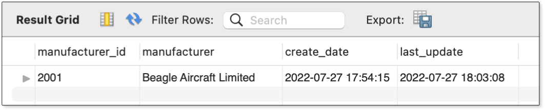
Figure 6 shows the data returned by this statement. As you can see, the table was updated with no problem, in part because you specified a new primary key value that did not already exist.

Figure 6. Updating the manufacturers table

You can also query the airplanes table to verify that the rows have been properly updated:

SELECT * FROM airplanes WHERE manufacturer_id = 2001;

Figure 7 shows the results returned by the query. As expected, the manufacturer_id values have been updated in all the target rows.

Figure 7. Updating the manufacturer_id column in the airplanes table

Chances are, you probably won’t have to update foreign key columns too frequently, but it’s good to understand what it takes to make it happen. Just know that there are other issues to be aware of, such as not trying to insert duplicate primary keys.

Updating primary key columns in MySQL tables

As with foreign keys, there might be times when you need to update the values in a primary key column. If you update a single value (as you saw above), it’s usually no problem as long as the new value conforms to the column’s requirements. However, things get trickier if updating multiple values at one time. For example, the following UPDATE statement attempts to add 1 to all plane_id values in rows that have a manufacturer_id value of 2001:

UPDATE airplanes 
SET plane_id = plane_id + 1
WHERE manufacturer_id = 2001;

The statement has a good chance of failing because of the order that MySQL updates each row of data (although you can never be certain about the exact order that the database engine will choose when updating data). This is because MySQL is trying to update the original value to a value that already exists and is itself waiting to be updated. For instance, if MySQL tries to update the first row from 342 to 343 before the second row has been changed, the statement will fail and MySQL will return the following error:

Error Code: 1062. Duplicate entry '343' for key 'airplanes.PRIMARY'

You might be tempted to include the IGNORE keyword to try to get around this issue:

UPDATE IGNORE airplanes 
SET plane_id = plane_id + 1
WHERE manufacturer_id = 2001;

The IGNORE keyword instructs MySQL to return a warning rather than an error and to continue with the statement’s execution instead of stopping. In this case, you’ll likely receive four warnings, along with a message indicating only one row was successfully updated:

1 row(s) affected, 4 warning(s):

1062 Duplicate entry '343' for key 'airplanes.PRIMARY'

1062 Duplicate entry '344' for key 'airplanes.PRIMARY'

1062 Duplicate entry '345' for key 'airplanes.PRIMARY'

1062 Duplicate entry '346' for key 'airplanes.PRIMARY'

Rows matched: 5 Changed: 1 Warnings: 4

If you query the airplanes table, you can see that only the last row has been updated, as shown in Figure 8. This is because the last row was the only one that did not try to update the primary key value to an existing value.

Figure 8. Using the IGNORE option when updating the plane_id column

A better solution is to include an ORDER BY clause that sorts the rows by the plane_id values, in descending order:

UPDATE airplanes 
SET plane_id = plane_id + 1
WHERE manufacturer_id = 2001
ORDER BY plane_id DESC;

When you include the ORDER BY clause in this way, MySQL applies the updates starting with the last row, making it possible to increment the values by 1 without generating any errors or warnings.

Figure 9 shows what the data now looks like after running the UPDATE statement.

Figure 9. Adding the ORDER BY clause to your UPDATE statement

You probably won’t need to use the ORDER BY clause very often, but when you do, it will prove very useful.

Another clause that’s similar in this respect is the LIMIT clause, which limits the number of rows that are updated. For instance, the following update statement limits the number of rows to 3:

UPDATE airplanes 
SET plane_id = plane_id + 1
WHERE manufacturer_id = 2001
ORDER BY plane_id DESC
LIMIT 3;

Because the UPDATE statement still includes the ORDER BY clause, the three rows that are updated start at the bottom and go up. Figure 10 shows the results of querying the table after the update.

Figure 10. Adding the LIMIT clause to your UPDATE statement

I suspect you’re not going to include the LIMIT clause in your UPDATE statements very often (if at all), but situations might arise in which you find it useful. For example, you might want to test an UPDATE statement that would normally modify a large number of rows. If you include the LIMIT clause while testing the statement, you’ll reduce the amount of time and processing it takes to verify that the statement is working properly.

Working with the MySQL UPDATE statement

The UPDATE statement is one of the most common statements used when working with MySQL data. In most cases, you’ll be including the UPDATE, SET and WHERE clauses. At times, you might forego the WHERE clause—at your own peril—and at other times, you might incorporate the ORDER BY clause or LIMIT clause (or both). However, the bulk of your updates will likely rely on the three primary clauses.

Regardless of which clauses you use, you should understand how they all work to ensure that you’re modifying your data as effectively as possible, while ensuring the accuracy of those updates. Fortunately, the UPDATE statement is fairly easy to understand and use, so you should have no problem getting started.

 

The post Introducing the MySQL UPDATE statement appeared first on Simple Talk.

from Simple Talk https://ift.tt/n8Frqto
via

Oracle optimizer Or Expansion Transformations

Jonathan Lewis' continuing series on the Oracle optimizer and how it transforms queries into execution plans:

1. Transformations by the Oracle Optimizer
2. The effects of NULL with NOT IN on Oracle transformations
3. Oracle subquery caching and subquery pushing
4. Oracle optimizer removing or coalescing subqueries
5. Oracle optimizer Or Expansion Transformations

There are two versions of this transformation, the “legacy” Or-Expansion – formerly known as “Concatenation” – and the new (12.2) implementation that allows Oracle greater scope and flexibility in its use. The basic mechanism is essentially the same in both versions though the shape of the execution plan does change. The key feature is that the optimizer can take a single query block and transform it into a UNION ALL of 2 or more query blocks which can then be optimized and run separately.

Here’s some code to create a table that I will use to demonstrate the principle:

create table t1
as
with generator as (
        select 
                rownum id
        from dual 
        connect by 
                level <= 1e4    -- > comment to avoid 
                                -- Wordpress format issue
)
select
        cast(rownum as number(8,0))                     id,
        cast(mod(rownum,1949) as number(8,0))           n1949,
        cast(mod(rownum,1951) as number(8,0))           n1951,
        cast(lpad(rownum,10,'0') as varchar2(10))       v1,
        cast(lpad('x',100,'x') as varchar2(100))        padding
from
        generator
order by
        dbms_random.value
;
create index t1_i1949 on t1(n1949);
create index t1_i1951 on t1(n1951);

The table t1 holds 10,000 rows. In case you’re wondering, 1949 and 1951 are prime numbers and since they are both slightly less than 2,000 most values in the two columns will appear 5 times each, but a few will appear six times. It’s worth doing a couple of quick queries to get a better intuitive feel for the data:

select  v1, n1949, n1951 from t1 where n1949 = 3;

select  v1, n1949, n1951 from t1 where n1951 = 3;

select  v1, n1949, n1951 from t1 where n1949 = 3 or n1951 = 3;

And here are the three sets of results from my test (in the absence of an “order by” clause your results may appear in a different order):

V1              N1949      N1951
---------- ---------- ----------
0000007799          3       1946
0000009748          3       1944
0000001952          3          1
0000005850          3       1948
0000000003          3          3
0000003901          3       1950

6 rows selected.

V1              N1949      N1951
---------- ---------- ----------
0000009758         13          3
0000005856          9          3
0000001954          5          3
0000007807         11          3
0000003905          7          3
0000000003          3          3

6 rows selected.

V1              N1949      N1951
---------- ---------- ----------
0000009758         13          3
0000005856          9          3
0000007799          3       1946
0000001954          5          3
0000007807         11          3
0000003905          7          3
0000009748          3       1944
0000001952          3          1
0000005850          3       1948
0000000003          3          3
0000003901          3       1950

11 rows selected.

You’ll notice, of course, that the two simple queries returned 6 rows, but the disjunct (“OR”) of the two separate predicates returned only 11 rows. A little visual inspection shows that the row where v1 = '0000000003' appears in both of the first two result sets when it’s only going to appear once in the final query.

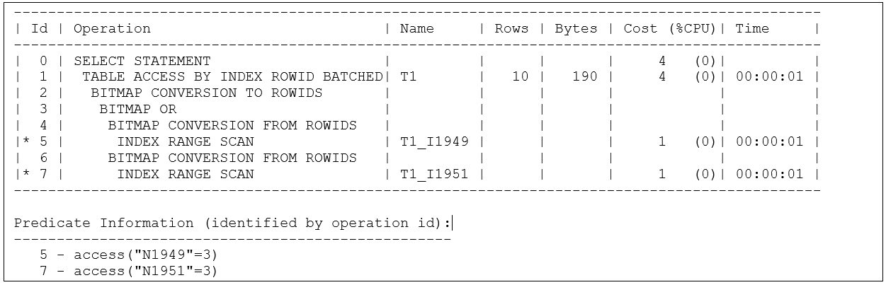
This example is so simple that the final plan doesn’t show OR expansion it has used a completely different option to access the data using a method that the optimizer thinks is cheaper (partly because of a limitation – not a bug – in the optimizer’s model). Here’s the plan (pulled from memory after checking the SQL_ID of the query):

select * from table(dbms_xplan.display_cursor('7ykzsaf3r0umb',null));

This returns:

The optimizer has decided to use btree/bitmap conversion. The plan does an index range scan of the two indexes, one for each predicate, then converts the two lists of rowids into two bit-strings, does a Bitmap-OR of the two strings then converts the resulting string back into a list of rowids. It’s an unfortunate feature of execution plans that bitmap strategies don’t include estimates of how many bits are “set” (i.e. 1) and how many rowids will be produced before showing the final estimate of rows returned after the table has been accessed by rowid and filtered.

Side note: Since the optimizer has no idea how the pattern of bits in a bitmap is related to the scattering of data (and the clustering_factor of a bitmap index is simply a count of the number of bitmap chunks in that index) the optimizer simply makes a guess about the data scatter. Roughly speaking it assumes that 80% of the rows identified through a bitmap predicate will be very well clustered, and that the remaining 20% will be widely scattered. Inevitably the resulting cost estimate of using the bitmap approach will be far too high in some cases and far too low in others.

Or-Expansion plans

Since the example allows the optimizer to use btree/bitmap conversion, the query will need a hint to disable that choice. Unfortunately, there’s no explicit hint to switch the mechanism off (you can force it to appear with the /*+ index_combine(alias) */ hint but there’s no “no_index_combine()” hint), so it’s necessary to fall back on the opt_param() hint to modify one of the optimizer parameters for the duration of the query.

Since I’m running 19.11.0.0 I’m going to run two more versions of the sample query – the first simply disables the btree/bitmap feature, the second also takes the optimizer back to the 12.1.0.2 optimizer feature level:

select  /*+ opt_param('_b_tree_bitmap_plans','false') */  
        v1, n1949, n1951 
from    t1 
where   n1949 = 3 or n1951 = 3;

select  /*+ 
                opt_param('_b_tree_bitmap_plans','false') 
                optimizer_features_enable('12.1.0.2') 
        */ 
        v1, n1949, n1951 
from    t1 
where   n1949 = 3 or n1951 = 3;

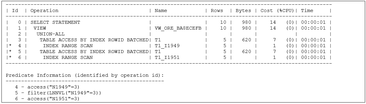
Here are the resulting plans – first the baseline 19.11.0.0 plan showing the newer Or-Expansion:

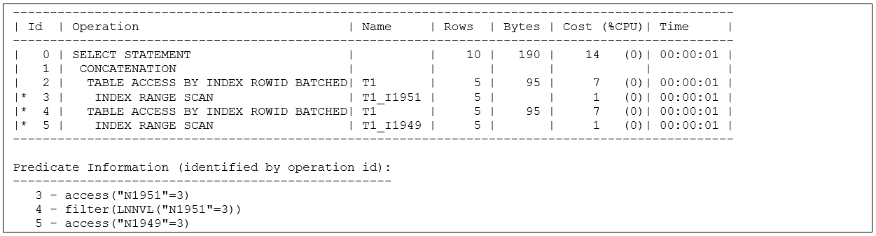
And here’s the 12.1.0.2 plan showing “Legacy” Or-Expansion (i.e. Concatenation):

 

The plans are clearly similar – both show two index range scans and the access predicate associated with each range scan uses the obvious index.

Both plans report an unusual filter predicate of the form lnnvl(column = constant) – and if you check the plan body and Predicate Information you’ll notice that this lnnvl() predicate is used during access to the second child of the Concatenation/Union All, but the “predicate within a predicate” echoes the predicate used during access to the first child of the plan. This is Oracle making sure that rows that were reported in the first part of the Concatenation/Union All do not get repeated by the second part.

The lnnvl() function takes a predicate as its single parameter, returning FALSE if the input predicate evaluates to TRUE, and TRUE if the predicate evaluates to FALSE or NULL. Effectively it is the “is not true()” function, engineered to work around some of the difficulties caused by SQL’s “three-value logic”.

There are several cosmetic differences between the plans – the view VW_ORE_xxxxxxxx makes it very clear that the plan includes Or-Expansion, and there’s an explicit UNION ALL operation that shows very clearly how Oracle is operating. One curious difference is the reversal of the order in which the original predicates become the separate branches of the transformed query – there doesn’t appear to be any clever arithmetic involved, it just seems to be a switch from bottom-up to top-down.

As a side note – this does mean that when you upgrade from a “Concatenation version” of Oracle” to Or-Expansion a query that you’ve written to “select first N rows” without including an “order by” clause may now return a different set of rows.

In effect, Or-Expansion has taken the original text and transformed it into a select from a UNION ALL view (text extracted from the CBO trace file and edited for readability – “test_user” was the name of the schema running the demo):

SELECT 
        VW_ORE_BA8ECEFB.ITEM_1 V1,
        VW_ORE_BA8ECEFB.ITEM_2 N1949,
        VW_ORE_BA8ECEFB.ITEM_3 N1951 
FROM    (
           (
           SELECT T1.V1 ITEM_1, T1.N1949 ITEM_2, T1.N1951 ITEM_3
           FROM TEST_USER.T1 T1 
           WHERE T1.N1949=3
           )
           UNION ALL
           (
           SELECT T1.V1 ITEM_1, T1.N1949 ITEM_2, T1.N1951 ITEM_3 
           FROM TEST_USER.T1 T1 
           WHERE T1.N1951=3 AND LNNVL(T1.N1949=3)
                )
        )       VW_ORE_BA8ECEFB
;

In more complex queries, of course, once this transformation has been done the optimizer may find ways other parts of the query can be transformed with the different query blocks embedded in this UNION ALL view. Again, this may cause some surprises when an upgrade takes you from Concatenation to Or-Expansion: plans may change because there are more cases where the optimizer can apply the basic expansion then carry on doing further transformations to individual branches of the UNION ALL.

Or-Expansion threats

A critical difference between Concatenation and Or-Expansion is that the OR’ed access predicates for the driving table must all be indexed before Concatenation can be used. The same restriction is not required for Or-Expansion and this means the optimizer will spend more time considering more execution plans while optimizing the query. Consider a query joining table tA and table tB with the following where clause:

SELECT  {list of columns}
FROM
        tA, tB
WHERE
        (tA.indexed_column = 'Y' or tA.unindexed_column = 'N')
AND     tB.join_column = tA.join_column
AND     tB.another_indexed_column = 'X'
;

This could be expanded to:

WHERE
         tA.indexed_column = 'Y'
AND      tB.join_column = tA.join_column
AND      tB.another_indexed_column = 'X'
...
UNION ALL
...
WHERE
         tA.unindexed_column = 'N'
AND      tB.join_column = tA.join_column
AND      tB.another_indexed_column = 'X'
AND      lnnvl(tA.indexed_column = 'Y')

This expansion would not be legal for Concatenation because (as indicated by the choice of column names) there is no indexed access path for the predicate tA.unindexed_column = ‘N’, but Or-Expansion would allow the transformation. At first sight that might seem like a silly choice – but now that the optimizer has two separate query blocks to examine, one of the options open to it is to produce a plan where the first query block uses an index into tA followed by a nested loop into tB while the second query block uses an index into tB followed by a nested loop into tA.

Generally we would expect the improved performance of the final plan to more than offset the extra time the optimizer spends investigating the extra execution plans but there are patterns where the optimizer tries too hard and things can go badly wrong; here’s an example from a few years ago that modelled a production performance problem:

drop table t1 purge;

CREATE TABLE t1
AS
WITH GENERATOR AS (
        SELECT  --+ materialize
                rownum id 
        FROM   dual 
        CONNECT BY 
                level <= 1e4
)
SELECT
        rownum          id1,
        rownum          id2,
        rownum          id,
        lpad(rownum,10) v1,
        rpad('x',100)   padding
FROM
        generator       v1,
        generator       v2
WHERE
        rownum <= 1e5   -- > comment to avoid 
                        -- wordpress format issue
;

CREATE INDEX t1_i1 ON t1(id1, id2);

SELECT * FROM t1 WHERE
   ( id1 =  1001 AND id2 in (1,2))
OR ( id1 =  1002 AND id2 in (2,3))
...
OR ( id1 =  1249 AND id2 in (249,250))
OR ( id1 =  1250 AND id2 in (250,251))
;

I’ve removed 246 lines from the query but you can probably see the pattern from the remaining 4 predicates. I didn’t write this query by hand, of course, I wrote a query to generate it. If you want to see the entire script (with some variations) you can find it at https://jonathanlewis.wordpress.com/2013/05/13/parse-time/

Running version 19.11 on my sandbox this query took 21.2 seconds to parse (optimize) out of a total run time of 22.1 seconds. The session also demanded 453 MB of PGA (Program Global Area) memory while optimizing the query. The execution plan was a full tablescan – but the optimizer spent most of its time costing Or-Expansion before discarding that option and picking a simple tablescan path.

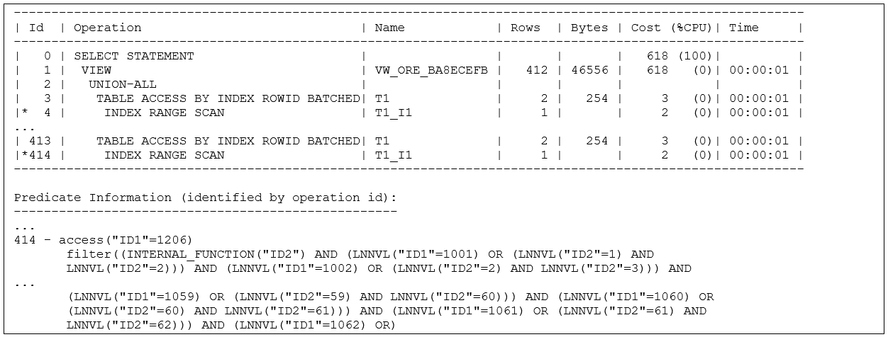
After a little trial and error I reduced the number of predicates to 206 at which point the plan switched from a full tablescan to using Or-Expansion (the cost was 618 for Or-Expansion and 619 for a hinted full tablescan, at 207 predicates the costs were 221 and 220 respectively). The counter-intuitive side effect of this change was to increase the optimization time to 27 seconds and the memory demand to 575MB. The reason for this was that having discovered that the initial OR-Expansion produced a lower cost than the tablescan the optimizer then evaluated a number of further transformations of the resulting UNION ALL view to see if it could produce an even lower cost.

Apart from the increase in the workload associated with the Or-Expansion another threat comes from an error in the estimate of CPU usage at actual run-time. Here are a few lines from the body of the execution plan with 206 predicates, and a few lines from the Predicate Information for just the last operation in the plan:

The plan includes 206 separate query blocks that do a basic index range scan with table access (I’ve shown just two of them) and as you work down the list the filter() predicate for each index range scan gets one more set of lnnvl() predicates than the previous one. In fact, by time the optimizer got to operation 128 – which is from the 63^rd query block in the Union All – the number of bytes allowed in v$sql_plan for reporting the filter predicate was too few to hold the entire predicate and, as you can see at the end of the sample above, the filter predicate has stopped at references to the values 61 and 62, and is nowhere near the values 206 and 207 which would have appeared in the last line of the original SQL statement. There’s a lot of lnnvl() checking that has to go on as the number of branches in the expansion increases – and that’s going to be burning up CPU at run-time.

To block the transformation and cut down the optimization time, all that was needed was the addition of the hint /*+ no_or_expand(@sel$1) */ to the query (sel$1 because I hadn’t used the qb_name() hint to give the query a programmer-friendly name) and this reduced the parse time from 27 seconds to 0.4 seconds and the memory demand to 7 MB.

Side note: It’s worth pointing out that when you run a query the memory used for optimization is in your PGA, and the memory you’re using will reduce the “aggregate PGA auto target” which affects the limit for every other user. On the other hand if you call “explain plan” to generate an execution plan without executing the query the memory used comes from the SGA (i.e. the shared pool), which means that when the optimizer goes a little mad with Or-Expansion your session may flush lots of useful information from the library cache, with far greater impact on the entire system. This is just one more reason for not depending on “explain plan” to give you execution plans.

If you’re responsible for the performance of a system, there are some clues about the overheads of optimization in extreme cases. One point to check is the active session history (ASH – v$active_session_history or dba_hist_active_sess_history) where you could aggregate SQLexecutions to check for statements that record more than one sample in a hard parse, e.g:

break on sql_id skip 1
select 
        sql_id, sql_exec_id, in_hard_parse, count(*) 
from 
        v$active_session_history 
group by 
        sql_id, sql_exec_id, in_hard_parse
having 
        count(*) > 1
order by 
        1,2,3

This returns

SQL_ID        SQL_EXEC_ID I   COUNT(*)
------------- ----------- - ----------
1v1mm1224up26             Y         18
2kt6gcu4ns3kq             N          2
                          Y         64
7zc0gjc4uamz6             Y         21
d47kdkn618bu4    16777216 Y          2
g1rvj7fumzxda    16777216 N          4

This isn’t a perfect search, unfortunately – if a statement is parsing, then it’s not yet executing so it doesn’t have an execution id (sql_exec_id), so when you see that sql_id“2kt6gcu4ns3kq” has recorded 64 samples “in hard parse” that might mean there have been lots of short hard parses (though that’s a little suspicious anyway) or a few long hard parses. You’d have to drill into sample times to get a better idea of what the larger numbers are telling you (64 consecutive sample times would be a fairly strong indication the statement was a threat).

Another thing you can check retrospectively is the alert log, as this may tell you about the memory aspect of extreme optimization problems. Here’s a short extract from my alert log following one of my nasty parse calls:

This isn’t saying anything about the hundreds of megabytes of PGA memory I’ve been using, it’s saying that someone pushed a “large object” into the SGA – but there’s a chance that an object that large is interesting and you’ll want to find out what it was, and the last few lines in the extract show that this one was an SQL statement that looks familiar. (The 51200K mentioned as the “notification threshold” is set by the hidden parameter _kgl_large_heap_warning_threshold.)

Summary

The Concatenation operation from earlier versions of Oracle has been superseded by the Or-Expansion operation, which is more flexible and can allow further transformations to be applied after the initial transformation in more ways than were available following the Concatenation operator. Or-Expansion is easily visible in execution plans, reporting a VIEW operation with a name like VW_ORE_xxxxxxxx followed by a UNION ALL operation.

On the plus side, some queries will be able to execute much more efficiently because the optimizer can find better plans for the different branches of the expansion; on the minus side the time spent in optimization can increase significantly and there will be cases where the cost of optimisation far outweighs the benefit of the faster execution. Although the CPU and elapsed time are the obvious costs of the optimization stage of Or-Expansion it is important to keep an eye on the demands for PGA that can also appear, so queries which have a large number of “OR’ed” predicates should be viewed with caution – and this includes queries with long “IN” lists, though the simplest type of IN-lists are likely to be transformed into “INLIST ITERATORS” rather than UNION ALL operations.

If you find cases where the optimizer persistently tries to use Or-Expansion when it’s a bad idea you can use the hint /*+ no_or_expand(@qbname) */ to block the expansion. The hint /*+ or_expand() */ is also available to force Or-Expansion (but it’s not a hint to use casually). If you aren’t allowed to block Or-Expansion through a hint or SQL patch then you could consider disabling the feature entirely by setting the hidden parameter _no_or_expansion to true at the system or session level.

The post Oracle optimizer Or Expansion Transformations appeared first on Simple Talk.

from Simple Talk https://ift.tt/LUCZpWq
via

Aha Moments at PASS Data Community Summit

Anyone who has attended Summit will recount tales of its wonderful ‘Aha!‘ moments. Perhaps it happens after a presentation, as you’re chatting in the lobby, when in a flash of inspiration an idea of how to tackle a problem suddenly reveals itself to you!

It may feel like a sudden flash, but more likely it’s the culmination of many small pockets of discovery; a day of learning in a pre-con, advice received in the Microsoft ‘tech zone’ of the Exhibition Hall, a casual chat at a Summit lunch, an interesting idea in a technical session. And now, as you stand in the lobby talking animatedly with a group of database people facing similar challenges, each of these disparate strands comes together and the solution is clear.

People tend to get misty-eyed when speaking of Summit, of the sense of community, the professional connections made, and long friendships forged. I’ve experienced this myself. However, if its value to you lies in building technical knowledge, and a strong professional network, the value to your employer depends on those ‘Aha!’ moments. These are the ones that will help you resolve the tough technical or architectural problem with which your team or organization is currently grappling.

The ‘hive mind’ can conjure some excellent ideas. We experience it occasionally on the best forum threads and discussions, but it really gets to work at a world event like PASS Data Community Summit. Here, you can network with DBAs and developers from across the globe, tackling similar problems in very different settings. You’ll hear new perspectives and fresh approaches to common problems. Often it will reveal the path you need to take.

If you’ve a good ‘Aha!’ moment from Summit, please share it! You can register for this year’s event here, and hopefully will provide a lot more of them.

The post Aha Moments at PASS Data Community Summit appeared first on Simple Talk.

from Simple Talk https://ift.tt/YWukOP1
via