Tuesday, November 22, 2022

Converting Data Across Time Zones: An In-Depth Primer

If only the entire world used UTC, wouldn’t life be so much easier? We can dream, can’t we? While some software applications can live in an ecosystem where all dates and times can be stored in a single time zone with no conversions needed, many cannot. As applications grow and interact more with international customers, this need becomes omnipresent.

Converting a current time from one time zone to another is relatively easy. Regardless of whether daylight savings is involved or not, one simply needs to retrieve the current time in both time zones, find the difference, and apply that difference as needed to date/time calculations. Historical data is trickier, though, as times from the past may cross different daylight savings boundaries.

This article dives into all the math required to convert historical times between time zones. While seemingly academic in nature, this information can be used when building applications that interact between time zones and need to apply detailed rules to those applications and their users. These calculations will be demonstrated in T-SQL and a function built that can help in handling the math for you.

Note that there are tools and functions that may be available to you that can convert time zone data automatically. For example, AT TIME ZONE in SQL Server 2016+ can do this. Not all data platforms have this available, though. Moreover, there is a huge benefit to understanding the nitty-gritty of how time zones are defined and how they work, even when tools are available to do the work for us.

The following is an example of how AT TIME ZONE can be used to quickly convert a point in time from on time zone to another:

SELECT
        CAST('3/1/2022 12:00:00' AS DATETIME2(0)) 
           AT TIME ZONE 'Eastern Standard Time' AS source_time,
        CAST('3/1/2022 12:00:00' AS DATETIME2(0)) 
           AT TIME ZONE 'Eastern Standard Time' 
             AT TIME ZONE 'Central European Standard Time' AS target_time,
        CAST('3/1/2022 12:00:00' AS DATETIME2(0)) 
           AT TIME ZONE 'Eastern Standard Time'
               AT TIME ZONE 'UTC' AS utc_time;

This T-SQL returns a time in Eastern Standard Time (3/1/2022 @ noon). The next time is the same one, but converted to Central European Time. The final time in the list is the same time converted to UTC. The inputs must be DATETIME2, or this syntax will fail. The results are as follows:

The results show the source time appended with the correct offset from UTC (-5 hours), the same time adjusted to Central European Time (+1 from UTC) and lastly the same time converted to UTC (with the expected offset of zero).

If AT TIME ZONE is available to you, consider using it as it is a relatively simple syntax that can help manage TIMEZONEOFFSET dates/times efficiently, without the need for extensive date math.

AT TIME ZONE does have some limitations, however. For example, a date from the 1800’s would still have modern daylight savings rules applied, even though daylight savings did not exist back then.

A Note on Changing Rules

And noted in the 1800’s example, daylight savings rules change. For example, in the United States, the period for daylight savings was lengthened by 5 weeks in 2007. Other countries have made similar changes over the years, with some abolishing the semi-annual time changes altogether. For the purpose of this article, and to avoid it getting far too complex, current rules will be honored in the examples, but the value of having T-SQL code that I will demonstrate is to allow you to be able to implement scenarios where the standard methods will not work.

If you have a need to accurately convert across boundaries when daylight savings rules (or any time zone rules for that matter) have changed, then add those breakpoints into your code as needed. These events are rare enough that they may not impact your code, and they are well-documented enough to be able to adjust for them effectively.

The simplest way to do this would be a versioned table that maintains time zone attributes and has a valid from/valid through date that indicates when each set of rules is applicable to a given time zone. Then any process that needs this data can consult the appropriate rules based on the date, filtering using the valid from/valid to dates.

Ideal Solutions to Time Zone Challenges

Understanding how time zones and daylight savings operate is invaluable to solving complex problems that arise when working with localized data. To some extent, avoiding these challenges altogether is next-to-impossible, but there are a wide variety of best practices that can minimize their impact and reduce the effort needed to resolve them.

Set Server Time to UTC

Having multiple moving targets can make working with data even more challenging. Data ultimately will reference two sets of time zones: The application data time zone and the server time zone. Having application and database servers set to UTC means that they have zero bias and never shift due to daylight savings. This greatly simplifies both code and database maintenance.

The most common problem that occurs when a database server is set to use a local time zone is when daylight savings shifts twice a year. What happens to SQL Server Agent Jobs when you spring forward and lose an hour from 02:00 to 03:00? The answer is that THEY NEVER RUN! For unsuspecting developers and administrators, this can be a nightmare. Imagine backups being skipped for a day. Or maybe a daily analytics job never crunches its data for an important dashboard. When daylight savings reverts to standard time, jobs scheduled during that hour to OCCUR TWICE (!) For some tasks, this may be acceptable, but a reporting task that creates data every hour may end up with duplicates. Similarly, any jobs that create files, backups, or tabular data will get an extra round of that data when this happens.

Any application that relies on SQL Server Agent or scheduled tasks that are scheduled using local server time will incur unexpected behavior when daylight savings shifts. The effort to mitigate this risk can be surprisingly complex to the point where some administrators simply avoid scheduling and all tasks during the daylight savings changeover time period (specified by standard_hour and daylight_hour). Similarly, a job that should run at midnight UTC will need to be adjusted alongside daylight savings changes if the server it resides on uses a non-UTC time zone. Otherwise, a job that runs at 8pm EST will become a job that runs at 01:00:00 UTC instead of 00:00:00 UTC when Eastern falls back to standard time.

If application and database servers can be set to UTC, then these problems disappear for good.

Store Date/Time data in UTC or DATETIMEOFFSET

When storing dates and times, the default often chosen when an application is new is the default local time zone. Over the years, this has resulted in many applications that use Eastern US or Pacific US time as the default format for storing this data. This seems convenient until an application grows to encompass many locales and inevitably becomes international, spanning dozens of countries and time zones. Now, conversions are needed to ensure that users see the correct time for where they live and internal processes can convert times correctly to enable meaningful data analytics. Similarly, a software development team may be scattered around many different time zones, adding more complexity into how dates/times are worked with.

Storing all dates and times in UTC ensures that no complex conversions are needed. This is simple and straightforward and if the database server is also set to UTC, then there is no discrepancy between SYSDATETIME() and SYSUTCDATETIME(). For some data points, such as log data, analytics, row versioning, or other internal processes, storing them in UTC is ideal for consistency and ease of use.

If data is directly correlated to a user or location that is time-sensitive, then storing that data using a DATETIMEOFFSET data type is ideal. DATETIMEOFFSET is a data type that stores a time along with its UTC offset. This provides the best of both worlds: the ability to quickly retrieve data points normalized to UTC (or some other time zone) and the ability to know what a local time is. Sometimes there is a need to understand what happens at certain times of day using local times, rather than UTC times. For example, analyzing how order processing occurs at a busy time of day is a common problem. Busy in London will occur at a different time of day than in Melbourne.

Do Not Make Assumptions

There are dozens of time zones defined around the world and they do not all operate the same way. Do not assume that the dates/times in your application will always behave like a specific time zone. Not only do different time zones behave differently from each other, but rules as to how time zones work can change over time.

Time zones should be seen as a property of the user experience. Time zones in of themselves are artificial constructs that help us navigate the day with more ease so that 12:00 is considered mid-day and is during a lighter part of the day, regardless of where you live. Computers do not care about time zones. Nor does data. Flying to Tokyo from New York does not cause you to travel forwards in time by crossing lots of time zones.

Therefore, treat time zones as if they are a user preference. If a user lives in Madrid, then they would experience the Central European time zone (UTC+2), but data stored about them may not need to know this. It could be UTC or DATETIMEOFFSET, if needed. Similarly, storing data in multiple time zones in a table is liable to result in confusion. Ideally, a column that represents a time should not require being stored repeatedly in many time zones. Those conversions should ideally happen in the presentation layer of an application and not in the database.

The Components of a Time Zone

Each time zone has built-in components that describe how it works. To understand how to convert between time zones, it is necessary to understand the components that comprise a time zone. These attributes can be roughly broken into two categories:

  1. How does this time zone compare to UTC?
  2. If this time zone uses daylight savings, how and when are adjustments made?

The following is a list of all components needed to understand the definition of a time zone:

Bias

This is the default difference between a time zone and UTC, typically given in minutes. It can be positive or negative. The number indicates the number of minutes that needs to be added to a local time to convert it into UTC during standard (non-daylight savings) times.

For example, a bias of zero indicates UTC/GMT. Eastern Standard time has a bias of 300, which indicates that 300 minutes need to be added to an Eastern Standard time (5 hours) to convert it to UTC during non-daylight savings times of the year. If daylight savings is in effect, then only 240 minutes would need to be added to the local time, though additional parameters related to daylight savings should be used to arrive at this number, since not all time zones behave the same way.

Start of Standard Time

For time zones with daylight savings, these numbers determine when during the year time is shifted from daylight savings back to standard time (aka: Fall Back). Along with the description will be the domain of values as they will be used in the code I will present.

  • Standard Month: The month of the year that time is shifted to standard time from daylight savings time. This is an integer from 1 (January) to 12 (December). Zero is typically used to denote time zones without daylight savings.
  • Standard Day: The day of the month after which daylight savings can occur. The day that daylight savings reverts is the first instance of the Standard Day of Week after the Standard Day. More on this below. This is an integer from 1-31. Zero is typically used to denote time zones without daylight savings.
  • Standard Day of Week: This is the day of the week that time shifts from daylight savings to standard time. This is an integer from 0 (Sunday) to 6 (Saturday) and has no meaning if this time zone does not have daylight savings.
  • Standard Hour: This is the hour of the day that time is shifted from daylight savings to standard time. This is an integer from 0 to 23 and has no meaning if this time zone does not have daylight savings.
  • Standard Bias: If there is any additional adjustment (in minutes) required to account for standard time, then it is provided here. Typically, this is zero and is not used in time zone calculations. For the purposes of this article, standard bias will not be used. Consider this a placeholder for hypothetical modifications introduced by future laws/changes, but as of the writing of this article is not used anywhere on Earth.

To determine when to shift from daylight savings to standard time, start with the standard month and day. If that day happens to be equal to the standard day of week, then you are done, otherwise iterate forward through the days of the month until the standard day of week is reached. For example, if the standard month is 11, the standard day is 1, and the standard day of week is 0 (Sunday), then that indicates that a time zone shifts from daylight savings to standard on the first Sunday of November, starting on November 1st. If November 1st is not a Sunday, then the shift will occur on the next Sunday of the month after November 1st. If the standard hour is 2, then the time will shift from daylight savings to standard time at 02:00 on that date.

Start of Daylight Saving Time

On the flip side, the following values provide the information needed to determine when and how to shift from standard time to daylight savings time. Time zones that do not use daylight savings are not impacted by these numbers.

  • Daylight Month: The month of the year that time is shifted to daylight savings time from standard time. This is an integer from 1 (January) to 12 (December). Zero is typically used to denote time zones without daylight savings.
  • Daylight Day: The day of the month after which time can shift from standard to daylight savings. The day that daylight savings occurs is the first instance of the Daylight Day of Week after the Daylight Day. This is an integer from 1-31. Zero is typically used to denote time zones without daylight savings.
  • Daylight Day of Week: This is the day of the week that time shifts from standard to daylight savings time. This is an integer from 0 (Sunday) to 6 (Saturday) and has no meaning if this time zone does not have daylight savings.
  • Daylight Hour: This is the hour of the day that time is shifted from standard to daylight savings time. This is an integer from 0 to 23 and has no meaning if this time zone does not have daylight savings.
  • Daylight Bias: This is the adjustment, in minutes, that occurs when time shifts from standard to daylight savings. This number can be positive or negative, but is usually negative and represents the minutes that are added to the local time zone bias to reach the daylight savings time. A time zone with a bias of 300 and a daylight bias of -60 indicates that when standard time shifts to daylight savings time, the local bias shifts to 240. In other words, this time zone “springs forward” an hour, as is often said colloquially.

The process to determine when to shift from standard to daylight savings time is quite similar to the process for shifting to standard time outlined earlier in this article. Start with the daylight month and day. This determines the earliest that daylight savings can occur. From here, the first instance of the daylight day of week (including that first date) is when daylight savings occurs. The daylight hour is the time when the daylight savings shift occurs. In most time zones, this is the same hour that is used for standard time.

Note that all time zone attributes are enumerated in Microsoft’s documentation and can be used when developing applications. More information can be found here: https://ift.tt/eFoIWl2

Many databases/lists of time zone attributes are available freely for download and use. The following is a small database containing a single table with the commonly used time zone metadata available for use. Feel free to download and share freely: https://www.dropbox.com/s/ifqflzqdhghifix/TimeZoneData.bak

There is a huge benefit to storing time zone information in a readily accessible table so that applications can use it whenever needed and have a centralized source of truth.

Example of Daylight Savings

Consider a time zone with the following parameters (this happens to be Pacific Standard Time):

  • Bias: 480 minutes (UTC-8)
  • Standard Month: 11 (November)
  • Standard Day: 1
  • Standard Day of Week: 0 (Sunday)
  • Standard Hour: 2
  • Daylight Month: 3 (March)
  • Daylight Day: 2
  • Daylight Day of Week: 0 (Sunday)
  • Daylight Hour: 2
  • Daylight Bias: -60 minutes

This time zone is UTC-8 hours (480 minutes). Daylight savings occurs on the first Sunday in March on or after March 2nd, at 02:00. At that time, 60 minutes are subtracted from this time zone’s bias, resulting in a new bias of 420 minutes (UTC-7 hours).

Similarly, this time zone reverts from daylight savings to standard time on the first Sunday in November on or after November 1st at 02:00. At that time, 60 minutes are added to this time zone’s bias to return it to its standard bias of 480 minutes (UTC-8 hours)

The Time Zone Challenge

Without daylight savings time, converting between time zones would simply be a matter of adjusting the bias between two time zones. For example, adjusting from a time zone with a bias of 300 to a time zone with a bias of 180 would only require that 120 minutes be subtracted from its bias. Practically speaking, reducing a time zone’s bias equates to adding minutes to a time whereas increasing the bias subtracts minutes from the time.

Daylight savings adds a wrinkle into this equation. The time on December 1st and the time on July 1st within a single time zone may each be subject to a different bias due to daylight savings. As a result, converting between time zones requires knowing whether each time zone honors daylight savings and if either (or both) do, then what are the details of when those time shifts occur.

For example, in the Central European time zone (UTC+1/bias of -60 minutes), daylight savings adds an hour on the first Sunday on or after March 5th. Therefore, 09:00 on March 1st is UTC+1, but 09:00 on April 1st is UTC+2. While those times are sampled in the same physical location, they essentially belong to different time zones. If data from this time zone is stored in UTC and converted back to the local time zone at a later time using the standard bias of -60, the result would be 09:00 on March 1st and 10:00 on April 1st.

Storing times as DATETIMEOFFSET resolves this issue in its entirety and is the recommended solution. Most date/time values in most databases are not stored with the UTC offset inline, though, and are subject to a data sampling error across daylight savings boundaries. DATETIMEOFFSET allows both the time and time zone to be defined all at once. This leaves no ambiguity with regards to precisely what time it was and its relationship to UTC and other time zones.

Therefore, the challenge that we are set to tackle here is to be able to use the attributes of time zones to retroactively convert one time into another and account for daylight savings in the process. Using the information discussed thus far, this process will be encapsulated into a scalar function that can handle the work for us.

Using T-SQL to Automate Time Zone Calculations

A better solution to the time zone problem is a function that can be passed the parameters for each time zone and can then crunch the resulting time using what we have discussed thus far in this article. The details for each time zone can be stored in table to make for more reusable code and reduce the need to hard-code time zone attributes whenever this is needed. Generally speaking, a table that contains a wide variety of attributes and dimensions for all time zones can be useful for many other purposes as well. The value in codifying time zone details and then referencing only standard time zone names or abbreviations is that it greatly reduces the chances for typos or mistakes. This provides similar functionality to a calendar table in that regard.

If one of the time zones is UTC, then zeroes can be passed in for all of that time zone’s parameters, which can simplify this function if one side of the equation happens to always be UTC. Similarly, if the daylight bias is always -60, which is likely, then it can be omitted as well. The function below has a variety of defaults to help simplify calls to it when various attributes are irrelevant, not needed, or not specified.

CREATE FUNCTION dbo.fnConvertBetweenTimeZones
(       @source_datetime DATETIME2(3),-- The date/time that will be 
                                    --converted to the target time zone.
        @source_bias AS SMALLINT = 0, -- Defaults to UTC
        @source_standard_month AS TINYINT = 0, -- Defaults to UTC
        @source_standard_day AS TINYINT = 0, -- Defaults to UTC
        @source_standard_day_of_week AS TINYINT = 0, -- Defaults to UTC
        @source_standard_hour AS TINYINT = 0, -- Defaults to UTC
     -- Source_ parameters default to UTC/no daylight savings
        @source_daylight_month AS TINYINT = 0, 
        @source_daylight_day AS TINYINT = 0, 
        @source_daylight_day_of_week AS TINYINT = 0,
        @source_daylight_hour AS TINYINT = 0,
     -- Defaults to -60 (1 hour) if used
        @source_daylight_bias AS SMALLINT = -60, 
     -- Target_ parameters default to UTC
        @target_bias AS SMALLINT, 
        @target_standard_month AS TINYINT = 0,
        @target_standard_day AS TINYINT = 0,
        @target_standard_day_of_week AS TINYINT = 0,
        @target_standard_hour AS TINYINT = 0,
        @target_daylight_month AS TINYINT = 0,
        @target_daylight_day AS TINYINT = 0,
        @target_daylight_day_of_week AS TINYINT = 0,
        @target_daylight_hour AS TINYINT = 0,
        @target_daylight_bias AS SMALLINT = -60)
RETURNS DATETIME2(3)
AS
BEGIN
        DECLARE @target_datetime DATETIME2(3);
        DECLARE @difference_in_minutes SMALLINT;
        -- Calculate base difference between time zones.
        SELECT @difference_in_minutes = @source_bias - @target_bias;
        -- Determine if source time was affected by daylight savings
        IF @source_daylight_month <> 0
        BEGIN
                DECLARE @source_daylight_start DATETIME2(3);
                DECLARE @source_daylight_end DATETIME2(3);
                -- Calculate when daylight savings starts
                SELECT @source_daylight_start = 
              DATEFROMPARTS(DATEPART(YEAR, @source_datetime), 
                      @source_daylight_month, @source_daylight_day);
                WHILE DATEPART(DW, @source_daylight_start) - 1 <> 
                                        @source_daylight_day_of_week
                BEGIN
                      SELECT @source_daylight_start = DATEADD(DAY, 1, 
                                              @source_daylight_start);
                END
                -- Calculate when daylight savings ends
                SELECT @source_daylight_end = 
              DATEFROMPARTS(DATEPART(YEAR, @source_datetime), 
                      @source_standard_month, @source_standard_day);
                WHILE DATEPART(DW, @source_daylight_end) - 1 <>   
                                          @source_standard_day_of_week
                BEGIN
                        SELECT @source_daylight_end = DATEADD(DAY, 1, 
                                               @source_daylight_end);
                END
                -- Add the daylight savings modifier, if needed
          
              IF @source_daylight_start < @source_daylight_end 
              -- Typically Northern hemisphere
                
                BEGIN
                  IF @source_datetime >= 
                   DATETIMEFROMPARTS(DATEPART(YEAR, @source_daylight_start), 
                          @source_daylight_month, 
                         DATEPART(DAY, @source_daylight_start), 
                                     @source_daylight_hour, 0, 0, 0)
                        AND @source_datetime < 
                DATETIMEFROMPARTS(DATEPART(YEAR, @source_daylight_end), 
                          @source_standard_month, 
                         DATEPART(DAY, @source_daylight_end), 
                                     @source_standard_hour, 0, 0, 0)
                        BEGIN
                                SELECT @difference_in_minutes = 
                       @difference_in_minutes + @source_daylight_bias;
                        END
                END
                IF @source_daylight_start > @source_daylight_end 
               -- Typically Southern hemisphere
                BEGIN
                 IF @source_datetime >= 
                  DATETIMEFROMPARTS(DATEPART(YEAR, @source_daylight_start), 
                      @source_daylight_month, 
                      DATEPART(DAY, @source_daylight_start), 
                               @source_daylight_hour, 0, 0, 0)
                        OR @source_datetime < 
                  DATETIMEFROMPARTS(DATEPART(YEAR, @source_daylight_end), 
                       @source_standard_month, 
                       DATEPART(DAY, @source_daylight_end), 
                               @source_standard_hour, 0, 0, 0)
                        BEGIN
                                SELECT @difference_in_minutes = 
                        @difference_in_minutes + @source_daylight_bias;
                        END
                END
        END
        -- Determine if the target time was affected by daylight savings
        IF @target_daylight_month <> 0
        BEGIN
                DECLARE @target_daylight_start DATETIME2(3);
                DECLARE @target_daylight_end DATETIME2(3);
                -- Calculate when daylight savings starts
                SELECT @target_daylight_start = 
               DATEFROMPARTS(DATEPART(YEAR, @source_datetime), 
                      @target_daylight_month, @target_daylight_day);
                WHILE DATEPART(DW, @target_daylight_start) - 1 <> 
                                           @target_daylight_day_of_week
                BEGIN
                        SELECT @target_daylight_start = 
                    DATEADD(DAY, 1, @target_daylight_start);
                END
                -- Calculate when daylight savings ends
                SELECT @target_daylight_end = 
                DATEFROMPARTS(DATEPART(YEAR, @source_datetime), 
                        @target_standard_month, @target_standard_day);
                WHILE DATEPART(DW, @target_daylight_end) - 1 <> 
                                            @target_standard_day_of_week
                BEGIN
                        SELECT @target_daylight_end = 
                         DATEADD(DAY, 1, @target_daylight_end);
                END
                -- Add the daylight savings modifier, if needed
                IF @target_daylight_start < @target_daylight_end 
                 -- Typically Northern hemisphere
                BEGIN
                 IF @source_datetime >= 
                  DATETIMEFROMPARTS(DATEPART(YEAR, 
                                       @target_daylight_start), 
                       @target_daylight_month, 
                       DATEPART(DAY, @target_daylight_start), 
                                       @target_daylight_hour, 0, 0, 0)
                        AND @source_datetime < 
                  DATETIMEFROMPARTS(DATEPART(YEAR, @target_daylight_end), 
                       @target_standard_month, 
                       DATEPART(DAY, @target_daylight_end), 
                                       @target_standard_hour, 0, 0, 0)
                        BEGIN
                                SELECT @difference_in_minutes = 
                        @difference_in_minutes - @target_daylight_bias;
                        END
                END
                IF @target_daylight_start > @target_daylight_end 
             -- Typically Southern hemisphere
                BEGIN
                        IF @source_datetime >= 
                 DATETIMEFROMPARTS(DATEPART(YEAR, @target_daylight_start), 
                      @target_daylight_month, 
                      DATEPART(DAY, @target_daylight_start), 
                                        @target_daylight_hour, 0, 0, 0)
                OR @source_datetime < 
                   DATETIMEFROMPARTS(DATEPART(YEAR, @target_daylight_end), 
                   @target_standard_month, 
                   DATEPART(DAY, @target_daylight_end), 
                                         @target_standard_hour, 0, 0, 0)
                        BEGIN
                                SELECT @difference_in_minutes = 
                          @difference_in_minutes - @target_daylight_bias;
                        END
                END
        END
        SELECT @target_datetime = 
             DATEADD(MINUTE, @difference_in_minutes, @source_datetime);
        RETURN @target_datetime;
END;

This function performs the following steps in order to convert @source_datetime to the target time zone:

  1. Determine the difference between time zones due to the difference in bias.
  2. If the source time zone observes daylight savings, then:
    • Determine when daylight savings begins for the source time zone.
    • Determine when daylight savings ends for the source time zone.
    • For time zones where the daylight savings month is before the standard month, apply the daylight bias, if needed. This is typically for time zones in the Northern hemisphere.
    • For time zones where the daylight savings month is after the standard month, apply the daylight bias, if needed. This is typically for time zones in the Southern hemisphere.
  3. If the target time zone observes daylight savings, then:
    • Determine when daylight savings begins for the target time zone.
    • Determine when daylight savings ends for the target time zone.
    • For time zones where the daylight savings month is before the standard month, apply the daylight bias, if needed. This is typically for time zones in the Northern hemisphere.
    • For time zones where the daylight savings month is after the standard month, apply the daylight bias, if needed. This is typically for time zones in the Southern hemisphere.
  4. Apply the calculated difference in minutes to the target datetime and return it.

Consider the following example:

SELECT dbo.fnConvertBetweenTimeZones('3/1/2022 12:00:00', 
             300, 11, 1, 0, 2, 3, 2, 0, 0, -60, -60, 10, 
             5, 0, 3, 3, 5, 0, 0, -60) AS target_time;

This code is converting noon on March 1st, 2022 from Eastern US time to Central European time. Both time zones observe daylight savings, but neither is observing it at this time. EST is UTC – 5 and CET is UTC + 1. The result of this function call is as follows:
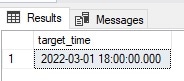
The results show that six hours were added to the source datetime. Since neither time zone was observing daylight savings, the time shift required only adding up the difference in biases and applying it to the date/time. In this case, 300 minutes from the source plus 60 additional minutes from the target, or 360 minutes (6 hours).

To test a scenario where one time zone is in daylight savings while the other is not, the following example can be used:

SELECT dbo.fnConvertBetweenTimeZones('6/1/2022 12:00:00', 
             300, 11, 1, 0, 2, 3, 2, 0, 0, -60, 0, 0, 
             0, 0, 0, 0, 0, 0, 0, 0) AS target_time;

This converts from Eastern Daylight Savings Time to UTC, with the result being as follows:
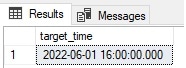
The bias for Eastern Time is 300 minutes, but is offset by -60 due to daylight savings, resulting in a bias of -240 minutes. This equates to UTC-4 and therefore to convert to UTC requires adding 4 hours to the source datetime, resulting in a conversion from 12:00 to 16:00 on the same date.

We can apply the dummy test case of converting a time from the same time zones to each other:

SELECT dbo.fnConvertBetweenTimeZones('7/1/2022 12:00:00', 
             480, 11, 1, 0, 2, 3, 2, 0, 0, -60, 480, 11, 
              1, 0, 2, 3, 2, 0, 0, -60) AS target_time;

Converting 7/1/2022 12:00:00 from PST to PST results in the following datetime:
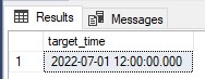
No surprise here, but this does provide a good QA test case to ensure that things are working the way they are expected to.

A common application of a function like this would be to apply it to a set of data from a table, rather than a hard-coded scalar value. The following query against WideWorldImporters converts the LastEditedWhen DATETIME2 column from Central time to UTC:

SELECT
        Orders.OrderID,
        Orders.LastEditedWhen,
        dbo.fnConvertBetweenTimeZones(Orders.LastEditedWhen, 
                    360, 11, 1, 0, 2, 3, 2, 0, 0, -60, 0, 0, 0, 0, 0, 
                    0, 0, 0, 0, 0) AS edited_time_from_CST_to_UTC
FROM WideWorldImporters.Sales.Orders
WHERE Orders.LastEditedWhen BETWEEN '3/2/2013' AND '4/4/2013'
ORDER BY Orders.LastEditedWhen, Orders.OrderID;

Note that this sample database from Microsoft may be downloaded for free from this link. This example intentionally intersects the time when Central time shifts from standard to daylight savings. The results illustrate that shift:
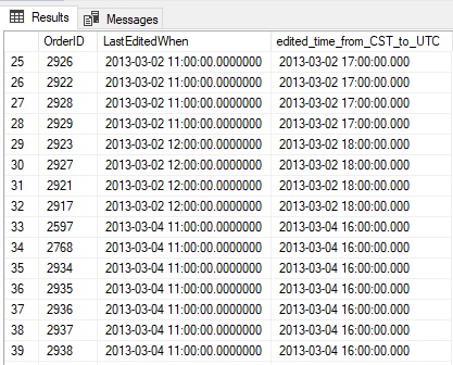
Note that the offset from Central US time to UTC changes from 6 hours to 5 hours after daylight savings goes into effect. The additional daylight bias of -60 minutes is added to the overall bias for Central time (360 minutes/6 hours) resulting in a new bias of 300 minutes (5 hours).

If time zone data is stored in a permanent reference table, then that table can be joined into the query to allow for a more dynamic approach based on the source/target time zones, removing most of the hard-coded literals and replacing them with column references within the time zone table.

What Else Can This be Used for?

The knowledge of how times work can be greatly helpful when working with code that does not already manage dates and times perfectly. Legacy code, T-SQL from older SQL Server versions, or code that needs to work across different data platforms may not be managed so easily.

The metadata that describes time zones can be used on its own as a reference tool to understand when and how daylight savings changes occur. They can also be used to gauge the time difference between two locations. The need to do this effectively arises often, even in systems where time zones are handled relatively well.

While the idea of regularly changing clocks to manage daylight savings has been losing appeal over the years, it is likely to remain in effect in many locales for years to come. If changes are made to remove it in a time zone or country, knowing how to adjust for future dates can allow applications to effectively prepare for future change, even before software updates are issued throughout the many tools and services we rely on to build, maintain, and host them.

Conclusion

Understanding how time zones and daylight savings works will make working with localized data much easier. If an application can be architected to minimize the need to convert between time zones, then doing so will avoid a wide variety of challenges and problems in the future. If an application cannot avoid this due to legacy data structures or code, then formalize how to convert between time zones and use the knowledge of how to represent time zones using their various attributes to provide the most reliable processes possible for managing multiple time zones.

The code in this article may not be needed in all scenarios, but will provide insight into the complexities of time zone conversions, especially with historical data. Use it as a way to better encapsulate metadata about time zones into a single source-of-truth and then build code that works with time zone data to be as re-usable as possible. This will improve code quality, reduce errors, and make an application more maintainable in the long run!


The post Converting Data Across Time Zones: An In-Depth Primer appeared first on Simple Talk.


from Simple Talk https://ift.tt/8mZyKEi
via

Monday, November 21, 2022

SQL Server 2022: Azure AD Authentication

SQL Server 2022 is finally GA and one of the features I was most expecting is finally available. It’s the allows Azure AD Authentication. Azure AD users can access SQL Server directly, without a second user account.

SQL Server on premises requires Azure ARC to be integrated to Azure. Azure VMs, on the other hand, don’t allow the usage of Azure ARC. Microsoft waited until the last moment to enable the same feature on the SQL Server IAAS Agent Extension.

Azure creates the SQL Server IAAS Agent Extension automatically for us when we create a SQL Server virtual machine. It appears as an additional Virtual Machine object. Using this object, we can control many details of SQL Server configuration inside an azure virtual machine and one of these details is the authentication method.


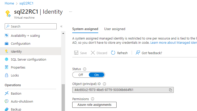
The first requirement for the Azure AD authentication is to set an identify to the virtual machine. On the Virtual Machine, we access the Identity tab and turn on the System Assigned Managed Identity. Azure will create an identity to the VM with the same name as the VM.


Define the Identity Permissions

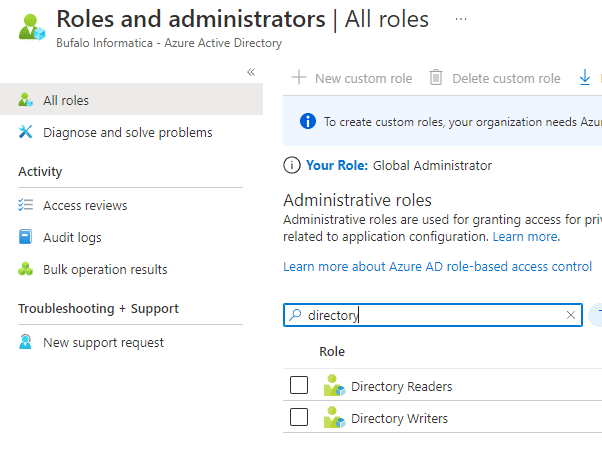
The VM identity needs permission to access active directory for authentication. We can set this permission by assigning the role Directory Readers to the VM account. Follow these steps to set the permissions:

1) Access Azure Active Directory

2) Click the Role and Administrators tab

3) On the search text box, type “Directory” to locate the directory readers role


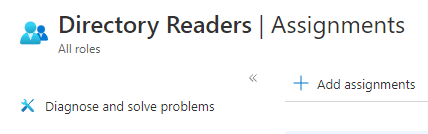
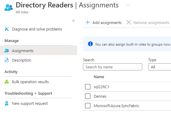
4) Click the Directory Readers role

5) Click the Add assignments button

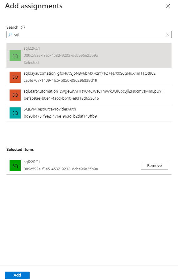
6) Locate the VM identity and click the add button


Set the Azure Authentication in SQL Server 2022

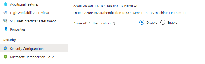
After these steps, we can enable the Azure AD Authentication on the SQL Server IaaS agent following these steps:

7) Access the Security Configuration tab


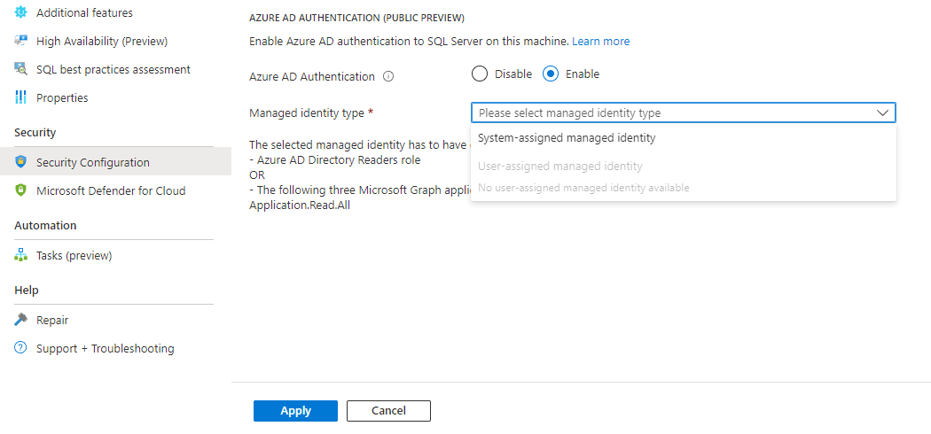
8) Click the Enable option

9) On the Managed identity type drop down, select the identity to be used.


10) Click the Apply button

Finally, we need to give permission to Azure users to access SQL Server. We need to use SSMS to set the permissions to the Azure users. The statements are simple:

CREATE login [dennes@dennesbufaloinfocom.onmicrosoft.com] FROM EXTERNAL provider
ALTER server role sysadmin ADD member
[dennes@dennesbufaloinfocom.onmicrosoft.com] 


Of course, you will adapt the role of your users according to your need. On Azure SQL Databases we can only create users from Azure if we are connected with an Azure account. SQL Server 2022 on an Azure VM doesn’t have this requirement.

Conclusion

SQL Server 2022 is the most cloud connected SQL Server version. Most of the connected features depend on Azure ARC, but Microsoft left for the last minute to enable the features through the SQL Server IaaS agent. One example that this was a last minute feature is how difficult it is to find documentation about this configuration.


The post SQL Server 2022: Azure AD Authentication appeared first on Simple Talk.


from Simple Talk https://ift.tt/fYFRCTh
via

Saturday, November 19, 2022

Backing up MySQL Part 3: mysqlpump

In the MySQL world, there are a couple of ways to take backups of your data. Backups in MySQL can be categorized into two distinct categories: logical or physical. MySQL also comes with a lot of tools helping us achieve our backup objectives: we have walked you through one of the most popular offerings in this space – Percona XtraBackup – in the second part of this series, and the first part of this series covered one of the main logical MySQL backup tools called mysqldump. As far as backups are concerned, though, we are far from done – for example, mysqldump alone has a brother called mysqlpump. Since the two CLI-based backup tools are frequently confused with each other, the aim of this blog is to clear the confusion up a little.

What is mysqlpump?

mysqlpump is a backup utility that is used via the command-line interface. The tool is very similar to mysqldump in that it provides us with the ability to take logical backups, but also different at the same time – the goal of mysqlpump is to be an extendable, parallel-supporting replacement of mysqldump. In their blog from 2015, MySQL team said that one of the primary aims of introducing mysqlpump was not be forced to implement legacy functionality that is provided by mysqldump.

mysqlpump was introduced to the world of MySQL in 2015 – the tool was added to MySQL 5.7.8.

Using mysqlpump

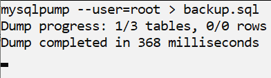
The most basic use case of mysqlpump looks like this (the tool can be used in the same fashion both on Linux and on Windows):

mysqlpump is designed in such a way that it will only dump tables that were created by a user – in other words, it will refrain from backing up tables that were created internally by MySQL (it won‘t touch any of the internal tables.)

The one feature that is exclusive to mysqlpump, though, is the ability to issue backups using multiple threads at once – to figure out how many threads your system has, follow these steps:

  1. Linux users – issue a command like lscpu or lscpu | egrep ‘Thread|CPU\(s\)’ and look at the output (you should see something similar to “Thread(s) per core.”)
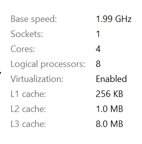
  2. Windows users – open up task manager and look at the number next to “Logical processors” – they represent the amount of threads in the system:

Once you know the number of threads in your system, think about the number of threads you wish (and can) allocate to mysqlpump – things might seem difficult and complex, but your thought process shouldn’t take more than a couple of seconds – mysqlpump is usually quick to complete too.

Once you know the number of threads in your infrastructure, configure the number of threads that can be used together with mysqlpump. Threads are to be configured using the --default-parallelism and --parallel-schemas options. Also, consider providing the username and password that you’re using to access MySQL itself through my.cnf for secure access: passwords provided through the CLI can be observed by accessing the history of issued commands. If you don’t want to do that, feel free to provide a username and a password, but be aware that mysqlpump itself will issue you warnings if you do so:

mysqlpump --default-parallelism=[threads] > data.sql

Since the “specialty” of mysqlpump is to back up data using multiple threads, we can also define the number of threads that we want the tool to use to dump a specific database – this functionality of mysqlpump can be exceptionally useful if we’re working with bigger sets of data, but need a logical backup to be taken.

mysqlpump – the Details

  • To specify more threads to dump a large database and less threads for smaller databases, look at the option named parallel-schemas. If you define your parameters like so, 6 threads will be used for larger databases, and 2 for smaller ones:
    mysqlpump --parallel-schemas=6:large_db1,large_db2 --parallel_schemas=2:small_db [--default-parallelism=x] > backup.sql
    Note the --default-parallelism option: a default number of threads when dumping other databases (databases that are not defined) can also be specified.
  • To back up only specific databases, define your query like so (here db_1 and db_2 represent two separate databases):
    mysqlpump –-databases db_1 db_2 > databases.sql
    You can also accomplish the same goal like so:
    mysqlpump --include-databases=db_1,db_2 --result-file=dump.sql
  • mysqlpump can also perform an “empty” dump (meaning that it can only back up the schema of the database, but not the data contained within):
    mysqlpump --include-databases=data_1,db2,db3 --skip-dump-rows --result-file=mydata.sql
  • mysqlpump also gives us the ability to use wildcards inside of any parameter. That means that if we have a lot of databases, backing a part of them (only those starting with the letter x, for example) is a breeze:
    mysqlpump --include-databases=x% --result-file=s_databases.sql
  • We can also exclude databases from being backed up like so (the following query would exclude all databases starting with test_ and back up all the rest):
    mysqlpump --exclude-databases=test_% --result-file=data.sql
  • We can also work with entire patterns (the following query would exclude all tables matching the demo pattern from the beginning):
    mysqlpump --exclude-tables=__demo --result-file=backup.sql
  • And last but not least, mysqlpump is also able to work with events and routines – all the same, just specify events or routines instead of databases and tables:
    mysqlpump --[include|exclude]-[events|routines]=title1,title2 --result-file=verycoolbackup.sql

mysqlpump can do a number of other things as well – all of the information on mysqlpump, as with everything MySQL-related, can be found at the documentation.

The Downsides of mysqlpump

However, as powerful as mysqlpump is, it’s also not without its weaknesses. Research made by Giuseppe Maxia back in September 2015 suggests that mysqlpump is faster than mysqldump, but only slightly – the blogger provides an example where mysqldump takes 3 minutes and 33 seconds to execute, whereas mysqlpump takes 2 minutes and 55 seconds – the difference is there, but we presume that the blogger has expected it to be way bigger than it was.

The research was made with approximately 20 million rows inside of the tables in the database – a figure big enough for both scripts to handle, but not large enough to invoke SELECT * INTO OUTFILE (a command used to back up bigger sets of data.) This suggests that mysqlpump is good if we find ourselves needing to use specific options not available to mysqldump, but doesn’t provide much of an upside otherwise.

Summary

mysqlpump entered the MySQL scene in 2015 with the release of MySQL 5.7.8. At first it was thought that it could be a reliable replacement for mysqldump and also offer a couple of “exotic” options not available to its counterpart, but as time went by mysqlpump proved that it still needs more refinement to be considered a reliable replacement for mysqldump.

Both mysqldump and mysqlpump are part of the MySQL’s ecosystem to this day, yet people steer towards mysqldump more than they do towards mysqlpump – while mysqlpump has its use cases, it is thought that its speed is not significant enough to outweigh its counterpart.

We hope that you’ve enjoyed reading this article, stay around the Redgate blog to learn more about everything database-related, and until next time.

The post Backing up MySQL Part 3: mysqlpump appeared first on Simple Talk.


from Simple Talk https://ift.tt/NP4qAgi
via

Thursday, November 17, 2022

Backing Up MySQL Part 2: Percona XtraBackup

There’s no doubt about it – if you’ve ever heard of Percona, you’ve heard of XtraBackup as well. XtraBackup is one of the primary Percona’s offerings in the backup space: the tool is famous amongst DBAs as one of the primary open-source utilities to take hot backups. The tool is known to avoid locking databases during its backup procedures – of course, it has a couple of limitations unique to itself, but that’s not an obstacle for experienced database administrators across the globe: the tool is loved by pretty much everyone who uses it, and with Percona at its side, we all know that the tool is going to deliver awesomeness by day and by night.

What is Percona XtraBackup?

As already stated above, Percona XtraBackup is one of the primary offerings for MySQL & Percona database administrators developed by Percona. The tool is an open-source backup utility that does not lock our databases during the backup processes it performs. Percona says that their tool can provide automatic verification of backups that have been taken, offer fast dumping and restore times, and above all, it’s supported by their award-winning consulting services helping us make sure that our data and its backups are in safe hands by day and by night.

How To Use Percona XtraBackup?

In order to start exploring the features offered by Percona’s XtraBackup, please install the tool before proceeding any further – the tool can be installed from a repo, from a tarball, from packages, or via source code – the old-fashioned way of installing the tool from a repository is a favourite option for many. To install the tool from a repo, head over to Percona’s documentation, and once you’re done installing, you can backup your data by issuing the command below (the command below will perform a full backup of your database, and then store the backup in a directory named “backups”):
xtrabackup --backup --target-dir=/backups

Bear in mind that in this case, contrary to mysqldump, the “backups” directory won’t consist of only one file – Percona’s XtraBackup would backup the following:

  • The my.cnf file that consists of the most vital information for MySQL to function correctly (XtraBackup will take a backup of the file and name it backup-my.cnf)
  • The file vital for InnoDB to function correctly – ibdata1. Since ibdata1 holds data, indexes, Multiversion Concurrency Control (MVCC) data, and double write & insert buffers that are necessary for InnoDB to work in the way it does, without it InnoDB’s infrastructure would plummet to ashes.
  • All databases inside of your MySQL infrastructure including the test and performance_schema databases.

Incremental backups can also be made in a very similar fashion: first, take a full backup using the command provided above, then issue a very similar statement, just add a --incremental-basedir statement at the end of it like so:
xtrabackup --backup --target-dir=/backups –incremental-basedir=/incbackups

In order to take a compressed backup, add the --compress option, and for partial backups, use one or more of the following options:

  • Use the --databases or --databases-file options to back up a database or a list of databases from a file:
    xtrabackup --databases=”db1 db2 test_db demo_db”
    xtrabackup --databases-file=databases.txt*
    * The file databases.txt would need to contain databases and tables in the format of database.table.
  • Use the --tables or --tables-file options to back up a table or a list of tables in the same fashion you would back up databases.

Woohoo – you’ve now learned how to take backups using Percona XtraBackup! That’s not everything, though – when using Percona XtraBackup you would also find yourself needing to prepare your backups for them to be successfully restored: we will tell you how to do that in the next section.

Preparing XtraBackups

As you could have noticed, Percona XtraBackup doesn’t take backups in a simple backup.sql form you might be used to when using mysqldump or other database backup tools – instead, Percona XtraBackup often takes a backup of the files associated with the database with itself too (we have covered those in the previous chapter.)

That’s why all of the backups taken using Percona XtraBackup need to be prepared for recovery before they can be successfully recovered – here’s how to do that for each flavour of backups:

  • To prepare a full or an encrypted backup to be restored, run the following command:
    xtrabackup --prepare --target-dir=backups/
  • To prepare an incremental backup to be recovered, you would need to ensure that the rollback phase will be skipped by specifying an --apply-log-only option. Percona themselves state that if the rollback phase isn’t prevented, the incremental backups would be worth nothing and you would have to start over, so keep that in mind. To prepare an incremental backup, run the same command as with full backups, just with the --apply-log-only option, nothing complex here:
    xtrabackup –apply-log-only –prepare –target-dir=backups/
  • To prepare a partial backup, specify the --export tag (don’t worry about warnings in this case – they are most likely issued because InnoDB “sees” tables, but their files do not exist in the data directory):
    xtrabackup --prepare --export --target-dir=backups/

And.. you’re done! Well, kind of. Now you also need to restore the backups, right?

Restoring XtraBackups

Now that you’ve made and prepared your backups, there will obviously be a point in time where you would need to restore what you’ve got in store. Again, such a process is a little different for each backup type, but don’t fret – we’re here to help. Here’s how to come around this issue:

  • To restore full, compressed, incremental, or encrypted backups, add a --copy-back option to restore your backup to the data directory:
    xtrabackup --copy-back --target-dir=/backups
  • To restore partial backups, all you have to do is restore all of the tables in the partial backup (copy them back to the server of your choice.)

That’s it – it’s that simple! Of course, we can run into a couple of issues during these steps as well, so it’s always beneficial to keep an eye out for the documentation.

Options Offered by Percona XtraBackup

As with everything command-line related, Percona XtraBackup has a couple of options associated with itself. Some of them are as follows (all of the options can be found over at the Percona’s documentation):

Percona XtraBackup Option

Meaning

--backup

Takes a backup of the database.

--check-privileges

Checks if Percona XtraBackup has all of the required privileges to be operating properly.

--apply-log-only

Prepares to take incremental backups by ignoring all stages except the redo stage.

--copy-back

Restores a backup. This option is meant to be used in conjunction with other options (see examples above.)

--databases=x | --tables=x

“x” specifies a database or a table inside of a database to be backed up. These options are similar to --databases-file or --tables-file options that backs up databases or tables from a file.

--defaults-file

Makes XtraBackup read only the options specified in the file after this parameter (the file will most likely be my.cnf.)

Summary

Percona XtraBackup is the flagship tool in Percona’s backup arsenal – the tool is widely used by junior and senior database administrators alike and as it avoids the locking of databases during its backup procedures, takes backups in a quick and safe fashion, and allows all kinds of backups to be restored quickly, there’s no doubt that Percona XtraBackup will be the option of choice for database engineers for many years to come. We hope that this blog post has provided you with some of the insight into the Percona’s XtraBackup world and that you will refer to the Percona’s manual for more information, and we will see you in the next blog!

The post Backing Up MySQL Part 2: Percona XtraBackup appeared first on Simple Talk.


from Simple Talk https://ift.tt/6bdQxzR
via

Saturday, November 12, 2022

Introducing the MySQL DELETE statement

Preparing your MySQL environment

As with the previous few articles, I used the same database and tables for the examples in this article (the travel database and the manufacturers and airplanes tables). In this case, however, I recommend that you start from scratch and rebuild the database and tables to keep things simple for this article. To set up the database, run the following script:

DROP DATABASE IF EXISTS travel;

CREATE DATABASE travel;

USE travel;

CREATE TABLE manufacturers (
  manufacturer_id INT UNSIGNED NOT NULL AUTO_INCREMENT,
  manufacturer VARCHAR(50) NOT NULL,
  create_date TIMESTAMP NOT NULL DEFAULT CURRENT_TIMESTAMP,
  last_update TIMESTAMP NOT NULL 
    DEFAULT CURRENT_TIMESTAMP ON UPDATE CURRENT_TIMESTAMP,
  PRIMARY KEY (manufacturer_id) )
ENGINE=InnoDB AUTO_INCREMENT=1001;

CREATE TABLE airplanes (
  plane_id INT UNSIGNED NOT NULL AUTO_INCREMENT,
  plane VARCHAR(50) NOT NULL,
  manufacturer_id INT UNSIGNED NOT NULL,
  engine_type VARCHAR(50) NOT NULL,
  engine_count TINYINT NOT NULL,
  max_weight MEDIUMINT UNSIGNED NOT NULL,
  wingspan DECIMAL(5,2) NOT NULL,
  plane_length DECIMAL(5,2) NOT NULL,
  parking_area INT GENERATED ALWAYS AS ((wingspan * plane_length)) STORED,
  icao_code CHAR(4) NOT NULL,
  create_date TIMESTAMP NOT NULL DEFAULT CURRENT_TIMESTAMP,
  last_update TIMESTAMP NOT NULL 
    DEFAULT CURRENT_TIMESTAMP ON UPDATE CURRENT_TIMESTAMP,
  PRIMARY KEY (plane_id),
  CONSTRAINT fk_manufacturer_id FOREIGN KEY (manufacturer_id) 
    REFERENCES manufacturers (manufacturer_id) ) 
ENGINE=InnoDB AUTO_INCREMENT=101;

Once you’ve created the database, you can add the sample data you’ll need to follow along with the exercises in this article. Start by running the following INSERT statement to add data to the manufacturers table:

INSERT INTO manufacturers (manufacturer)
VALUES ('Bombardier'), ('Beagle Aircraft Limited');

SELECT *
FROM   manufacturers;

The statement adds two rows to the manufacturers table and outputs those rows. The manufacturer_id column in those rows should have been assigned the values 1001 and 1002.

After you confirm the data in the manufacturers table, you should run the following INSERT statement, which populates the airplanes table:

INSERT INTO airplanes 
  (plane, manufacturer_id, engine_type, engine_count, 
    wingspan, plane_length, max_weight, icao_code)
VALUES
  ('Learjet 24',1001,'Jet',2,35.58,43.25,13000,'LJ24'),
  ('Learjet 24A',1001,'Jet',2,35.58,43.25,12499,'LJ24'),
  ('Challenger (BD-100-1A10) 300',1001,'Jet',2,63.83,68.75,38850,'CL30'),
  ('Challenger (BD-100-1A10) 350',1001,'Jet',2,69,68.75,40600,'CL30'),
  ('Challenger (CL-600-1A11) 600',1001,'Jet',2,64.33,68.42,36000,'CL60'),
  ('Challenger (CL-600-2A12) 601',1001,'Jet',2,64.33,68.42,42100,'CL60'),
  ('A.109 Airedale',1002,'piston',1,36.33,26.33,2750,'AIRD'),
  ('A.61 Terrier',1002,'piston',1,36,23.25,2400,'AUS6'),
  ('B.121 Pup',1002,'piston',1,31,23.17,1600,'PUP'),
  ('B.206',1002,'piston',2,55,33.67,7500,'BASS'),
  ('D.4-108',1002,'piston',1,36,23.33,1900,'D4'),
  ('D.5-108 Husky',1002,'piston',1,36,23.17,2400,'D5');

SELECT *
FROM   airplanes;

The values 1001 and 1002 from the manufacturers table provide the foreign key values for the manufacturer_id column in the airplanes table. After you run the second INSERT statement, the SELECT query will let you confirm that 12 rows have been added to the airplanes table. The first row should have been assigned 101 as the plane_id value, and the plane_id values for the other rows should have been incremented accordingly.

The DELETE statement syntax

The basic syntax for the DELETE statement is fairly straightforward and includes many of the same elements you saw in the other DML statements (INSERT and UPDATE article links):

DELETE [IGNORE] FROM table_name
[WHERE where_condition]
[ORDER BY order_list]
[LIMIT row_count]

The syntax shown here does not include all supported statement components, but it provides the basic elements you need to know to get started with the DELETE statement. You can refer to MySQL topic DELETE Statement for the complete syntax. In the meantime, here’s a breakdown of the statement’s clauses, as I’ve shown in the syntax:

  • The DELETE clause, which includes the FROM subclause, is the only mandatory clause in the DELETE statement. The clause identifies that table from which the data will be deleted. You can specify multiple tables, which involves defining join conditions, but my focus in this article is on single-table deletes. The DELETE clause also supports the use of the IGNORE modifier for returning a warning message, rather than an error, if an issue arises.
  • The WHERE clause determines which rows to delete, based on one or more search conditions. The clause works much like the WHERE clause in SELECT and UPDATE statements. Although the WHERE clause is optional, you should be very careful running a DELETE statement that does not include one. Without a WHERE clause, the statement will delete every row in the target table, unless the LIMIT clause is included.
  • The ORDER BY clause specifies the order that rows should be deleted. This clause is used primarily in conjunction with the LIMIT clause to help better direct which rows should be removed. The ORDER BY clause is similar to the one you saw in the SELECT and UPDATE statements. The clause is optional and cannot be used for multi-table deletes.
  • The LIMIT clause limits the number of rows that will be deleted. When used with the ORDER BY clause, the deleted rows will be determined by the sort order specified by that clause. As with the ORDER BY clause, the LIMIT clause is optional and cannot be used for multi-table deletes.

As you work through the examples in this article, you’ll get a better sense of how the various statement elements work together. That said, the clauses are, for the most part, self-explanatory, and for most uses, you should have little trouble figuring out how they work. The larger concern is that you can lose a lot of data if you’re not careful when using this statement, so always exercise caution, and be sure that all data is fully protected. Above all, make sure you’re not working in a production environment when learning how to use the DELETE statement.

Deleting data from a MySQL table

As noted above, the DELETE clause is the only mandatory clause in a DELETE statement. If you run a DELETE statement with only this clause, it will remove all of the data from the target table—a consideration that should not be taken lightly. If you determine that this is what you want to do, you need only specify the DELETE and FROM keywords, followed by the table name, as in the following example:

DELETE FROM airplanes;

The statement will delete all data from the airplanes table, unless safe mode is enabled. Safe mode is typically enabled by default on a MySQL instance to help limit the possibility of updating or deleting all data in a table.

Much the same as described for the UPDATE statement, if safe mode is enabled on your MySQL instance, you’ll receive the following error message when you try to run the above statement:

Error Code: 1175. You are using safe update mode and you tried to update a table without a WHERE that uses a KEY column. To disable safe mode, toggle the option in Preferences -> SQL Editor and reconnect.

When safe mode is enabled, you cannot run a DELETE statement without a WHERE clause that does not specify a key column in the WHERE clause criteria, unless you include a LIMIT clause. This helps to ensure that you don’t inadvertently delete a table full of data. You can disable safe mode (as the error message suggests) by setting the server properties or by temporarily disabling safe mode when you run the DELETE statement. The temporary approach is usually the safest.

To temporarily disable safe mode, use a SET statement to change the SQL_SAFE_UPDATES system variable to 0 prior to running your DELETE statement and then set the variable to 1 after running the statement, as shown in the following example:

SET SQL_SAFE_UPDATES = 0;

DELETE FROM airplanes;

SET SQL_SAFE_UPDATES = 1;

The SET statements toggle the system variable off and then on during the current session. When taking this approach, be aware that if your DELETE statement generates an error, statement execution will stop and the second SET statement will not execute, so make sure you run this statement to reset the SQL_SAFE_UPDATES variable to 1. Also note that the SET statement supports the optional GLOBAL modifier, which defines a variable at the global scope. However, I recommend that you do not use this option when disabling safe deletes. It is less risky to disable safe mode at the session level to avoid any inadvertent data modifications. Use GLOBAL only if it’s essential in your situation.

Once safe mode is disabled, you should be able to run your DELETE statement without generating an error. After you do, you can confirm your changes with a simple SELECT statement that retrieves all data from the airplanes table. The statement should return no rows.

Adding a WHERE clause to your DELETE statement

In most cases, you’ll want to include a WHERE clause in your DELETE statements so you can target which rows in a table should be deleted (as opposed to deleting all rows). The WHERE clause defines one or more search conditions that specify exactly what data to delete. To see how this works, you should first add the data back to the airplanes table (assuming you’re trying out these examples):

INSERT INTO airplanes 
  (plane, manufacturer_id, engine_type, engine_count, 
    wingspan, plane_length, max_weight, icao_code)
VALUES
  ('Learjet 24',1001,'Jet',2,35.58,43.25,13000,'LJ24'),
  ('Learjet 24A',1001,'Jet',2,35.58,43.25,12499,'LJ24'),
  ('Challenger (BD-100-1A10) 300'
               ,1001,'Jet',2,63.83,68.75,38850,'CL30'),
  ('Challenger (BD-100-1A10) 350'
                ,1001,'Jet',2,69,68.75,40600,'CL30'),
  ('Challenger (CL-600-1A11) 600'
                ,1001,'Jet',2,64.33,68.42,36000,'CL60'),
  ('Challenger (CL-600-2A12) 601'
               ,1001,'Jet',2,64.33,68.42,42100,'CL60'),
  ('A.109 Airedale',1002,'piston',1,36.33,26.33,2750,'AIRD'),
  ('A.61 Terrier',1002,'piston',1,36,23.25,2400,'AUS6'),
  ('B.121 Pup',1002,'piston',1,31,23.17,1600,'PUP'),
  ('B.206',1002,'piston',2,55,33.67,7500,'BASS'),
  ('D.4-108',1002,'piston',1,36,23.33,1900,'D4'),
  ('D.5-108 Husky',1002,'piston',1,36,23.17,2400,'D5');

SELECT *
FROM airplanes;

Confirm that the data has been re-added to the airplanes table by looking at the output of the SELECT statement. The table should now be populated with the same 12 rows, with one notable difference. The first plane_id value is now 113 rather than 101 because MySQL tracks the last auto-incremented value that was assigned to a row, even if that row has been deleted.

After you’ve inserted the data into the airplanes table, you can run the following DELETE statement, which includes a basic WHERE clause:

DELETE FROM airplanes
WHERE icao_code = 'pup';

The search condition specifies that the icao_code value must equal pup for a row to be deleted. However, if you try to run this statement and safe mode is enabled, MySQL will again return error 1175:

Error Code: 1175. You are using safe update mode and you tried to update a table without a WHERE that uses a KEY column. To disable safe mode, toggle the option in Preferences -> SQL Editor and reconnect.

MySQL returns this error because the WHERE clause does not include a key column in its search condition. To get around this, you can again temporarily disable safe mode at the session level:

SET SQL_SAFE_UPDATES = 0;

DELETE FROM airplanes
WHERE icao_code = 'pup';

SET SQL_SAFE_UPDATES = 1;

If you query the airplanes table after running these statements, the table should now include only 11 rows rather than 12. Only one row satisfied the search condition, so only that row was deleted.

In cases where you specifically know what rows to delete, you should try to use a key column in your search condition to avoid having to disable safe mode. For example, the row deleted in the previous example had a plane_id value of 121. As a result, you could have recast the DELETE statement as follows:

DELETE FROM airplanes
WHERE plane_id = 121;

Of course, it’s not always practical to use a key column, in which case, you should define the WHERE clause in a way that best suits your situation, even if it means specifying multiple search conditions, as in the following example:

SET SQL_SAFE_UPDATES = 0;

DELETE FROM airplanes
WHERE engine_type = 'piston' AND max_weight < 2500 ;

SET SQL_SAFE_UPDATES = 1;

Because the WHERE clause contains no key column, safe mode must again be disabled during the session.

The WHERE clause itself includes two search conditions. The first one specifies that the engine_type value must be piston, and the second one specifies that the max_weight value must be less that 2500. The search conditions are connected by the AND logical operator, which means that both conditions must evaluate to true for a row to be deleted.

In this case, several rows matched both search conditions, so they were all removed from the airplanes table. If you query the table, you should find that it now includes only eight rows.

Adding ORDER BY and LIMIT clauses to your DELETE statement

Together, the ORDER BY and LIMIT clauses help you better control how rows are deleted from a table. To see how this works, start be adding a row back into the airplanes table:

INSERT INTO airplanes 
  (plane, manufacturer_id, engine_type, engine_count, 
    wingspan, plane_length, max_weight, icao_code)
VALUES
  ('D.4-108',1002,'piston',1,36,23.33,1900,'D4');

Because this row is being added separately from when the previous rows were added, it will have a different create_date value from the other rows. (The value is a timestamp.) You can use this value to single out the row when building your DELETE statement:

DELETE FROM airplanes
ORDER BY create_date DESC
LIMIT 1;

Notice that the statement includes no WHERE clause with a key column and that there are no SET statements. You can get away with this here because the DELETE statement includes a LIMIT clause. If necessary, you can include a WHERE clause with the ORDER BY and LIMIT clauses, but it’s not needed in this case.

The ORDER BY clause specifies that the rows should be deleted based on the create_date values, sorted in descending order. This ensures that the last row inserted is the first row deleted, assuming it has a unique create_date value. The LIMIT clause then specifies that only one row should be deleted. This will be the first row as it is determined by the ORDER BY clause. You might also consider this approach when deleting archived data, except that you would likely specify an amount other than 1 in the LIMIT clause, such as 100, 1000, or another value.

It’s hard to say how often you’ll use the ORDER BY and LIMIT clauses in your queries. But it’s good to know that you have this option if you want to apply similar logic when deleting data from your database tables.

You can also use these clauses independently of each other. For example, you might use the LIMIT clause when you need to delete a large number of rows from a table and you’re concerned about the impact on database performance. Instead of deleting all the rows at once, you can delete them in batches based on the number of rows specified in the LIMIT clause. Then you can simply rerun the DELETE statement until all the target rows have been removed.

Using the IGNORE modifier in your DELETE statement

As noted earlier, the DELETE statement supports the use of the optional IGNORE modifier, which you also saw in the INSERT and UPDATE statements. When IGNORE is used, your DELETE statement will return a warning rather than an error if an issue arises. In addition, MySQL will continue with the statement execution. If you don’t use IGNORE, MySQL will return an error and stop all statement execution, including any statements in the batch that follow the DELETE statement.

To see how this works, start by running the following INSERT statement, which adds several rows to the manufacturers table:

INSERT INTO manufacturers (manufacturer)
VALUES ('Airbus'), ('Beechcraft'), ('Cessna'), ('Piper');

SELECT *
FROM   manufacturers;

From the output of this batch, you should find that the Airbus row has a manufacturer_id value of 1003. You will use this value as the foreign key value when you add a row to the airplanes table for an Airbus plane. To add the row, run the following INSERT statement:

INSERT INTO airplanes 
  (plane, manufacturer_id, engine_type, engine_count, 
    wingspan, plane_length, max_weight, icao_code)
VALUES
('A220-100',1003,'Jet',2,115.08,114.75,134000,'BCS1');

Suppose you now want to delete all the rows you recently added to the manufacturers table. You might try to run the following DELETE statement, using the manufacturer_id values for those rows:

DELETE FROM manufacturers
WHERE manufacturer_id IN (1003, 1004, 1005, 1006);

When you try to run this statement, MySQL stops statement execution and returns the following error, which indicates you have a foreign key violation:

Error Code: 1451. Cannot delete or update a parent row: a foreign key constraint fails (`travel`.`airplanes`, CONSTRAINT `fk_manufacturer_id` FOREIGN KEY (`manufacturer_id`) REFERENCES `manufacturers` (`manufacturer_id`))

MySQL returned this error because you tried to delete a row that was being referenced by the airplanes table. As a result, the entire statement failed and no rows were deleted. However, you can ensure that the DELETE statement continues to execute even if one of the deletions fails by including the IGNORE modifier:

DELETE IGNORE FROM manufacturers
WHERE manufacturer_id IN (1003, 1004, 1005, 1006);

Now the statement returns the following message, which shows the number of rows that have been affected and provides a warning:

3 row(s) affected, 1 warning(s): 1451 Cannot delete or update a parent row: a foreign key constraint fails (`travel`.`airplanes`, CONSTRAINT `fk_manufacturer_id` FOREIGN KEY (`manufacturer_id`) REFERENCES `manufacturers` (`manufacturer_id`))

From this message, you can see that three rows have been deleted and that there has been a foreign key violation. If you query the manufacturers table, you’ll find that it now contains only three rows, including the one for Airbus. To remove all the Airbus data, you must first delete any referencing records from the airplanes table:

DELETE FROM airplanes
WHERE manufacturer_id = 1003;

You should then be able to run the following DELETE statement to remove the Airbus record from the manufacturers table, which will leave you with only two rows in that table:

DELETE  FROM manufacturers
WHERE manufacturer_id = 1003;

The IGNORE modifier can be useful when you need to schedule a deletion and want the statement execution to continue even if some rows cannot be deleted. This could be especially useful when deleting large sets of data. After the bulk of records have been deleted, you can go back and address any warnings. Be aware, however, that the IGNORE modifier works for only certain types of errors.

Working with the MySQL DELETE statement

The DELETE statement, along with the SELECT, INSERT, and UPDATE statements, represent four of the most important statements you’ll use when working with MySQL data. However, they’re not the only DML statements. MySQL also supports DML statements such as CALL, LOAD DATA, REPLACE, and TABLE.

But the four we’ve covered so far in this series are a great place to start for manipulating data, with the DELETE statement helping to complete that picture. The statement makes it possible to easily remove data that is incorrect or outdated. In fact, the statement can be almost too easy to use, and you must be careful not to inadvertently delete the wrong data. That said, the DELETE statement is extremely useful, and you should be sure that you fully understand how to use it, along with the SELECT, INSERT, and UPDATE statements.


The post Introducing the MySQL DELETE statement appeared first on Simple Talk.


from Simple Talk https://ift.tt/8lqiUrj
via

Friday, November 11, 2022

Optimizing MySQL: The Basics of Query Optimization

MySQL is a very interesting beast to deal with – both junior developers and expert database administrators working with the RDBMS know that the world of MySQL offers a breadth of opportunities not found anywhere else: people can choose a storage engine to use from a list of powerful storage engines, the RDBMS can be heavily optimized to serve very specific needs, MySQL has multiple specific types of tools and operations in place that can be used to optimize query performance, etc.

One of the most frequent causes of headaches for database administrators for ages are queries and their optimization for speed. As old as this question is, it’s still very hot. Have a skim through database-related questions posted on StackOverflow within the present week – do you see any patterns? “Slow query…”, “Performance Improvement…“, “Indexing strategy for..”, “Preventing toxic selects”, “Database not using index.” All of those questions mean one thing – issues concerning database performance are still very important, and people want to know how best to work with their queries to achieve the best mix of performance, availability, security, and capacity.

In the upcoming series, we’re focusing on the optimization of MySQL – we’re going to walk you through storage engine and query optimization, we’re going to tell you a couple of secrets situated around MySQL optimization settings, how best to measure performance, amongst other things. We’re starting small – in this blog, we’re walking you through the basics of the basics and answering the age-old question – why are my queries slow?!

Why Your Queries Are Slow

MySQL offers a couple of types of queries we can choose from:

  • INSERT queries that insert data into our database;
  • SELECT queries that read through data;
  • UPDATE queries that update our data;
  • DELETE queries that delete data within our database;
  • ALTER queries that change (alter, hence the name) data within our database.

The main reasons those queries are slow are as follows:

  • INSERT queries are slow most likely because there is a lot of data to be inserted into the database or (and) because the database isn’t optimized properly.
  • SELECT queries are slow mainly because they read through a lot of unnecessary data. The less data there is to scan through, the faster our SELECT queries will become. That’s it – there’s no rocket science involved.
  • UPDATE queries are usually slow because we either have an index on the column that is being updated or we are executing a huge update query without familiarizing ourselves with the internals of storage engines – InnoDB usually locks the table when UPDATEs are being performed and unlocks it after the fact.
  • DELETE queries might be slow because of an index on the column that we’re deleting the data from or because we’re deleting massive amounts of data without knowing the internals of storage engines as well. However, unlike UPDATE queries, DELETE queries have a couple of tricks up their sleeve – they can be massively sped up if we use the TRUNCATE query to remove all of the rows at once, then reimport only the necessary data.
  • ALTER queries are usually slow because of improperly optimized operations that run internally:
    • ALTER queries first make a copy of the table.
    • Once the copy of the table is made, the data existing in the original table is copied into it.
    • All of the necessary changes are made.
    • The original table is swapped with the copy.

All of those operations consume time – time that must be accounted for.

Some of such operations can be optimized for performance by properly adjusting the buffer pool used by the InnoDB storage engine, others can be optimized by adding or removing the presence of indexes and partitions, and all of them can be optimized by understanding the internals of queries available within MySQL. For now, though, understand one thing – queries are processes comprised of tasks, and to optimize the performance of those processes, we must optimize the tasks within those processes.

We hope that you’ve enjoyed reading this article and that it helped you grasp the basics of query optimization in the database management system of MySQL – stay tuned to learn how to optimize tasks within processes, read our blog to learn about database management systems in more detail, and until next time.

The post Optimizing MySQL: The Basics of Query Optimization appeared first on Simple Talk.


from Simple Talk https://ift.tt/wniH16e
via