Subqueries in MySQL

Part of Robert Sheldon's continuing series on Learning MySQL. The series so far:

1. Getting started with MySQL
2. Working with MySQL tables
3. Working with MySQL views
4. Working with MySQL stored procedures
5. Working with MySQL stored functions
6. Introducing the MySQL SELECT statement
7. Introducing the MySQL INSERT statement
8. Introducing the MySQL UPDATE statement
9. Introducing the MySQL DELETE statement

With that in mind, let’s dive into the subquery and take a look at several different ones in action. In this article, I focus primarily on how the subquery is used in SELECT statements to retrieve data in different ways from one table or from multiple tables. Like the previous articles in this series, this one is meant to introduce you to the basic concepts of working with subqueries so you have a solid foundation on which to build your skills. Also like the previous articles, it includes a number of examples to help you better understand how to work with subqueries so you can start using them in your DML statements.

Preparing your MySQL environment

For the examples in this article, I used the same database and tables that I used for the previous article. The database is named travel and it includes two tables: manufacturers and airplanes. However, the sample data I use for this article is different from the last article, so I recommend that you once again rebuild the database and tables to keep things simple for this article’s examples. You can set up the database by running the following script:

DROP DATABASE IF EXISTS travel;

CREATE DATABASE travel;
USE travel;
CREATE TABLE manufacturers (
  manufacturer_id INT UNSIGNED NOT NULL AUTO_INCREMENT,
  manufacturer VARCHAR(50) NOT NULL,
  create_date TIMESTAMP NOT NULL DEFAULT CURRENT_TIMESTAMP,
  last_update TIMESTAMP NOT NULL 
    DEFAULT CURRENT_TIMESTAMP ON UPDATE CURRENT_TIMESTAMP,
  PRIMARY KEY (manufacturer_id) )
ENGINE=InnoDB AUTO_INCREMENT=1001;

CREATE TABLE airplanes (
  plane_id INT UNSIGNED NOT NULL AUTO_INCREMENT,
  plane VARCHAR(50) NOT NULL,
  manufacturer_id INT UNSIGNED NOT NULL,
  engine_type VARCHAR(50) NOT NULL,
  engine_count TINYINT NOT NULL,
  max_weight MEDIUMINT UNSIGNED NOT NULL,
  wingspan DECIMAL(5,2) NOT NULL,
  plane_length DECIMAL(5,2) NOT NULL,
  parking_area INT GENERATED ALWAYS AS ((wingspan * plane_length)) STORED,
  icao_code CHAR(4) NOT NULL,
  create_date TIMESTAMP NOT NULL DEFAULT CURRENT_TIMESTAMP,
  last_update TIMESTAMP NOT NULL 
    DEFAULT CURRENT_TIMESTAMP ON UPDATE CURRENT_TIMESTAMP,
  PRIMARY KEY (plane_id),
  CONSTRAINT fk_manufacturer_id FOREIGN KEY (manufacturer_id) 
    REFERENCES manufacturers (manufacturer_id) ) 
ENGINE=InnoDB AUTO_INCREMENT=101;

After you’ve created the database, you can add the sample data so you can follow along with the exercises in this article. Start by running the following INSERT statement to add data to the manufacturers table:

INSERT INTO manufacturers (manufacturer)
VALUES ('Airbus'), ('Beagle Aircraft Limited'), ('Beechcraft'), ('Boeing'), 
  ('Bombardier'), ('Cessna'), ('Dassault Aviation'), ('Embraer'), ('Piper');

The statement adds nine rows to the manufacturers table, which you can confirm by querying the table. The manufacturer_id value for the first row should be 1001. After you confirm the data in the manufacturers table, you can run the following INSERT statement to populate the airplanes table, using the manufacturer_id values from the manufacturers table:

INSERT INTO airplanes 
  (plane, manufacturer_id, engine_type, engine_count, 
    wingspan, plane_length, max_weight, icao_code)
VALUES
  ('A340-600',1001,'Jet',4,208.17,247.24,837756,'A346'),
  ('A350-800 XWB',1001,'Jet',2,212.42,198.58,546700,'A358'),
  ('A350-900',1001,'Jet',2,212.42,219.16,617295,'A359'),
  ('A380-800',1001,'Jet',4,261.65,238.62,1267658,'A388'),
  ('A380-843F',1001,'Jet',4,261.65,238.62,1300000,'A38F'),
  ('A.109 Airedale',1002,'Piston',1,36.33,26.33,2750,'AIRD'),
  ('A.61 Terrier',1002,'Piston',1,36,23.25,2400,'AUS6'),
  ('B.121 Pup',1002,'Piston',1,31,23.17,1600,'PUP'),
  ('B.206',1002,'Piston',2,55,33.67,7500,'BASS'),
  ('D.5-108 Husky',1002,'Piston',1,36,23.17,2400,'D5'),
  ('Baron 56 TC Turbo Baron',1003,'Piston',2,37.83,28,5990,'BE56'),
  ('Baron 58 (and current G58)',1003,'Piston',2,37.83,29.83,5500,'BE58'),
  ('Beechjet 400 (same as MU-300-10 Diamond II)',1003,'Jet',2,43.5,48.42,15780,'BE40'),
  ('Bonanza 33 (F33A)',1003,'Piston',1,33.5,26.67,3500,'BE33'),
  ('Bonanza 35 (G35)',1003,'Piston',1,32.83,25.17,3125,'BE35'),
  ('747-8F',1004,'Jet',4,224.42,250.17,987000,'B748'),
  ('747-SP',1004,'Jet',4,195.67,184.75,696000,'B74S'),
  ('757-300',1004,'Jet',2,124.83,178.58,270000,'B753'),
  ('767-200',1004,'Jet',2,156.08,159.17,315000,'B762'),
  ('767-200ER',1004,'Jet',2,156.08,159.17,395000,'B762'),
  ('Learjet 24',1005,'Jet',2,35.58,43.25,13000,'LJ24'),
  ('Learjet 24A',1005,'Jet',2,35.58,43.25,12499,'LJ24'),
  ('Challenger (BD-100-1A10) 350',1005,'Jet',2,69,68.75,40600,'CL30'),
  ('Challenger (CL-600-1A11) 600',1005,'Jet',2,64.33,68.42,36000,'CL60'),
  ('Challenger (CL-600-2A12) 601',1005,'Jet',2,64.33,68.42,42100,'CL60'),
  ('414A Chancellor',1006,'Piston',2,44.17,36.42,6750,'C414'),
  ('421C Golden Eagle',1006,'Piston',2,44.17,36.42,7450,'C421'),
  ('425 Corsair-Conquest I',1006,'Turboprop',2,44.17,35.83,8600,'C425'),
  ('441 Conquest II',1006,'Turboprop',2,49.33,39,9850,'C441'),
  ('Citation CJ1 (Model C525)',1006,'Jet',2,46.92,42.58,10600,'C525'),
  ('EMB 175 LR',1008,'Jet',2,85.33,103.92,85517,'E170'),
  ('EMB 175 Standard',1008,'Jet',2,85.33,103.92,82673,'E170'),
  ('EMB 175-E2',1008,'Jet',2,101.67,106,98767,'E170'),
  ('EMB 190 AR',1008,'Jet',2,94.25,118.92,114199,'E190'),
  ('EMB 190 LR',1008,'Jet',2,94.25,118.92,110892,'E190');

The manufacturer_id values from the manufacturers table provide the foreign key values needed for the manufacturer_id column in the airplanes table. After you run the second INSERT statement, you can query the airplanes table to confirm that 35 rows have been added. The first row should have been assigned 101 for the plane_id value, and the plane_id values for the other rows should have been incremented accordingly.

Building a basic scalar subquery

A scalar subquery is one that returns only a single value, which is then passed into the outer query through one of its clauses. The subquery is used in place of other possible expressions, such as a constants or column names. For example, the following SELECT statement (the outer query) includes a subquery in search condition of the WHERE clause:

SELECT plane_id, plane
FROM airplanes
WHERE manufacturer_id = 
  (SELECT manufacturer_id FROM manufacturers 
    WHERE manufacturer = 'Beechcraft');

The subquery is the expression on the right side of the equal sign, enclosed in parentheses. A subquery must always be enclosed in parentheses, no matter where it’s used in the outer statement.

Make certain that your subquery does indeed return only one value, if that’s what it’s supposed to do. If the subquery were to return multiple values and your WHERE clause is not set up to handle them (as in this example), MySQL will return an error letting you know that you messed up.

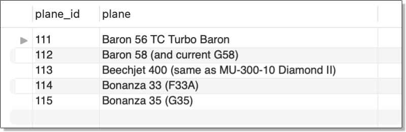
In this case, the subquery is a simple SELECT statement that returns the manufacturer_id value for the manufacturer named Beechcraft. This value, 1003, is then passed into the WHERE clause as part of its search condition. If a row in the airplanes table contains a manufacturer_id value that matches 1003, the row is included in the query results, which are shown in the following figure.

The subquery in this example retrieves data from a second table, in this case, manufacturers. However, a subquery can also retrieve data from the same table, which can be useful if the data must be handled in different ways. For example, the subquery in the following SELECT statement retrieves the average max_weight value from the airplanes table:

SELECT plane_id, plane, max_weight
FROM airplanes
WHERE max_weight > 
  (SELECT AVG(max_weight) FROM airplanes);

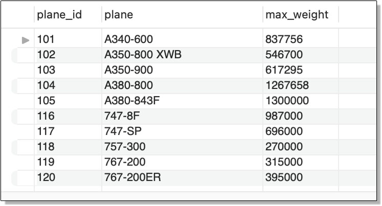
The WHERE clause search condition in the outer statement uses the average to return only rows with a max_weight value greater than that average. If you were to run the subquery on its own, you would see that the average maximum weight is 227,499 pounds. As a result, the outer SELECT statement returns only those rows with a max_weight value that exceeds 227,499 pounds, as shown in the following figure.

As I mentioned earlier in the article, you can use subqueries in statements other than SELECT. One of those statements is the SET statement, which lets you assign variable values. You can use a SET statement to define a value that can then be passed into other statements. For example, the following SET and SELECT statements implement the same logic as the previous example and return the same results:

SET @avg_weight = 
  (SELECT ROUND(AVG(max_weight)) FROM airplanes);
SELECT plane_id, plane, max_weight
FROM airplanes WHERE max_weight > @avg_weight;

The SET statement defines a variable named @avg_weight and uses a subquery to assign a value to that variable. This is the same subquery that is in the previous example. The SELECT statement then uses that variable in its WHERE clause (in place of the original subquery) to return only those rows with a max_weight value greater than 227,499 pounds.

The examples in this section focused on using scalar subqueries in SELECT statements, but be aware that you can also use them in UPDATE and DELETE statements, as well as the SET clause of the UPDATE.

Working with correlated subqueries

One of the most valuable features of a subquery is its ability to reference the outer query from within the subquery. Referred to as a correlated subquery, this type of subquery can return data that is specific to the current row being evaluated by the outer statement. For example, the following SELECT statement uses a correlated subquery to calculate the average weight of the planes for each manufacturer, rather than for all planes:

SELECT m.manufacturer_id, m.manufacturer, 
  a.plane_id, a.plane, a.max_weight
FROM airplanes a INNER JOIN manufacturers m
  ON a.manufacturer_id = m.manufacturer_id
WHERE a.max_weight > 
  (SELECT ROUND(AVG(max_weight)) FROM airplanes a2
    WHERE a.manufacturer_id = a2.manufacturer_id);

Unlike the previous two examples, the subquery now includes a WHERE clause that limits the returned rows to those with a manufacturer_id value that matches the current manufacturer_id value in the outer query. This is accomplished by assigning an alias (a) to the table in the outer query and using that alias when referencing the table’s manufacturer_id column within the subquery.

In this case, I also assigned an alias (a2) to the table referenced within the subquery, but strictly speaking, you do not need to do this. I like to include an alias for consistency and code readability, but certainly take whatever approach works for you.

To better understand how the subquery works logically (as opposed to how the optimizer might actually execute it), consider the first row in the airplanes table, which has a manufacturer_id value of 1001.

When the outer query evaluates the first row, it compares the max_weight value to the value returned by the subquery. To carry out this comparison, the database engine first matches the manufacturer_id value in the outer query to the manufacturer_id values returned by the subquery’s SELECT statement. It then finds all rows associated with the current manufacturer and returns the average max_weight value for that manufacturer, repeating the process for each manufacturer returned by the outer query.

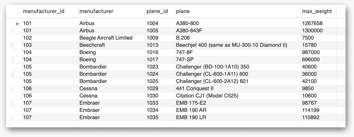
The following figure shows the results returned by the outer SELECT statement. The max_weight values are now compared only with the manufacturer-specific averages.

You can also use this same subquery in the SELECT clause as one of the column expressions. In the following example, I added the subquery after the max_weight column and assigned the alias avg_weight to the new column:

SELECT manufacturer_id, plane_id, plane, max_weight,
  (SELECT ROUND(AVG(max_weight)) FROM airplanes a2
    WHERE a.manufacturer_id = a2.manufacturer_id) AS avg_weight
FROM airplanes a
WHERE max_weight > 
  (SELECT ROUND(AVG(max_weight)) FROM airplanes a2
    WHERE a.manufacturer_id = a2.manufacturer_id);

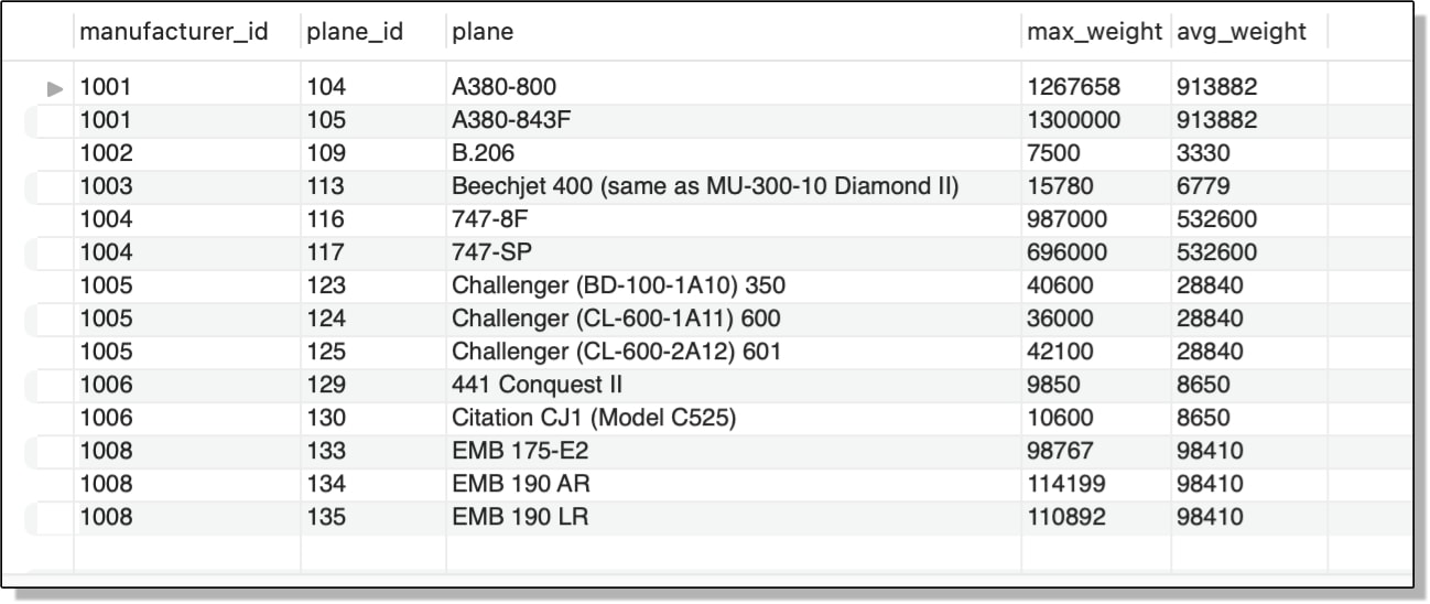
The new subquery works the same as in the preceding example. It returns the average weight only for the planes from the current manufacturer, as shown in the following figure.

In the previous example, I used a subquery to create a generated column. However, you can use a subquery when creating an even more complex generated column. In the following example, I’ve added a generated column named amt_over, which subtracts the average weight returned by the subquery from the weight in the max_weight column:

SELECT manufacturer_id, plane_id, plane, max_weight,
  (SELECT ROUND(AVG(max_weight)) FROM airplanes a2
    WHERE a.manufacturer_id = a2.manufacturer_id) AS avg_weight,
  -- subtracts average weight from max weight
  (max_weight - (SELECT ROUND(AVG(max_weight)) FROM airplanes a2
    WHERE a.manufacturer_id = a2.manufacturer_id)) AS amt_over
FROM airplanes a
WHERE max_weight > 
  (SELECT ROUND(AVG(max_weight)) FROM airplanes a2
    WHERE a.manufacturer_id = a2.manufacturer_id);

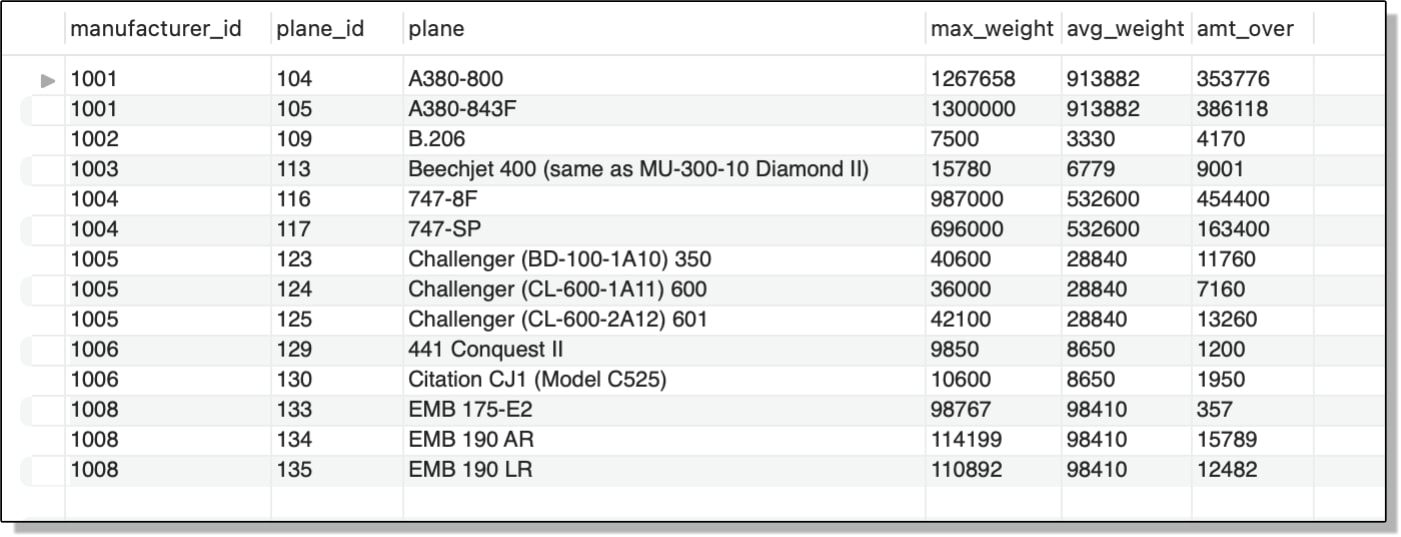
The avg_weight column in the SELECT list is a generated column that uses a subquery to return the average weight of the current manufacturer. The amt_over column is also a generated column and it uses the same subquery to return the average weight. Only this time, the column subtracts that average from the max_weight column to return the amount that exceeds the average.

The following figure shows the results now returned by the outer SELECT statement. As you can see, they include the amt_over generated column, which shows the differences in the weights.

If you want, you can also retrieve the name of the manufacturer from the manufacturers table and include that in your SELECT clause, as shown in the following example:

SELECT manufacturer_id, 
  (SELECT manufacturer FROM manufacturers m 
    WHERE a.manufacturer_id = m.manufacturer_id) manufacturer,
  plane_id, plane, max_weight,
  (SELECT ROUND(AVG(max_weight)) FROM airplanes a2
    WHERE a.manufacturer_id = a2.manufacturer_id) AS avg_weight,
  (max_weight - (SELECT ROUND(AVG(max_weight)) FROM airplanes a2
    WHERE a.manufacturer_id = a2.manufacturer_id)) AS amt_over
FROM airplanes a
WHERE max_weight > 
  (SELECT ROUND(AVG(max_weight)) FROM airplanes a2
    WHERE a.manufacturer_id = a2.manufacturer_id);

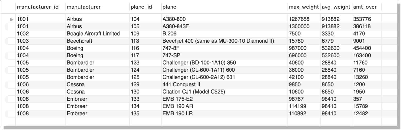
This statement is similar to the previous statement except that it adds the manufacturer column, a generated column. The new column uses a subquery to retrieve the name of the manufacturer from the manufacturers table, based on the manufacturer_id value returned by the outer query.

In some cases, a subquery might not perform as well as other types of constructs. For example, MySQL can often optimize a left outer join better than a subquery that carries out comparable logic. If you’re using a subquery to perform an operation that can be achieved in another way and are concerned about performance, you should consider testing both options under a realistic workload to determine which is the best approach.

The following figure shows the results with the additional column, which I’ve named manufacturer.

One other detail I want to point out about using subqueries in the SELECT list is that you can include them even if you’re grouping and aggregating data. For instance, the following SELECT statement includes a subquery that retrieves the name of the manufacturer associated with each group:

SELECT manufacturer_id, 
  (SELECT manufacturer FROM manufacturers m 
    WHERE a.manufacturer_id = m.manufacturer_id) manufacturer,
  COUNT(*) AS plane_amt
FROM airplanes a
WHERE engine_type = 'piston'
GROUP BY manufacturer_id
ORDER BY plane_amt DESC;

The subquery in this statement is similar to those you’ve seen in other examples, except that now you’re dealing with aggregated data, so the subquery must use a column that is mentioned in the GROUP BY clause of the outer statement, which it does (the manufacturer_id column). The statement returns the results shown in the following figure.

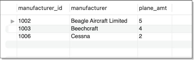
As you can see, the data has been grouped based on the manufacturer_id column, and the name of the manufacturer is included with each ID. In addition, the number of airplanes with piston engines is provided for each manufacturer, with the results sorted in descending order, based on that amount.

Working with a row of data

So far, all the examples in this article have returned scalar values, but your subqueries can also return multiple values, as noted earlier. For example, it might be useful to use a subquery to aggregate a table’s data, calculate specific averages in that data (returned as a single row), and then retrieve rows from the same table that exceed those averages, which is what I’ve done in the following SELECT statement:

SELECT 
  (SELECT manufacturer FROM manufacturers m 
    WHERE a.manufacturer_id = m.manufacturer_id) manufacturer,
        plane_id, plane, max_weight, parking_area,
  (SELECT ROUND(AVG(max_weight)) FROM airplanes a2
    WHERE a.manufacturer_id = a2.manufacturer_id) AS avg_weight,
  (SELECT ROUND(AVG(parking_area)) FROM airplanes a2
    WHERE a.manufacturer_id = a2.manufacturer_id) AS avg_area
FROM airplanes a
WHERE (max_weight, parking_area) > 
  (SELECT ROUND(AVG(max_weight)), ROUND(AVG(parking_area)) 
    FROM airplanes a2
    WHERE a.manufacturer_id = a2.manufacturer_id);

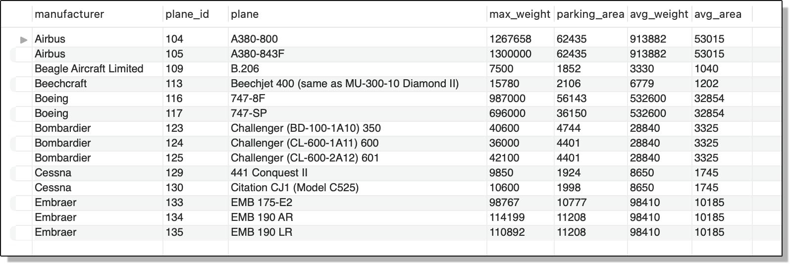
Notice that the WHERE clause in the outer statement includes the max_weight and parking_area columns in parentheses. In MySQL, this is how you create what is called a row constructor, a structure that supports simultaneous comparisons of multiple values. In this case, the row constructor is compared to the results from the subquery, which returns two corresponding values. The first value is the average weight, as you saw earlier. The second value returns the average parking area, which is based on the values in the parking_area column.

In both cases, the averages are specific to the current manufacturer_id value in the outer query. For the outer query to return a row, the two values in the row constructor must be greater than both corresponding values returned by the subquery. Notice also that the SELECT list now includes both the max_weight and parking_area columns, along with the average for each one. The outer statement returns the results shown in the following figure.

One thing you might have noticed about the subqueries in the preceding examples, particularly those used in the WHERE clauses, is that all the search conditions in those clauses use basic comparison operators, either equal (=) or greater than (>). However, you can use any of the other comparison operators, including special operators such as IN and EXISTS, as you’ll see in the next section.

Working with a column of data

The previous section covered row subqueries. A row subquery can return only a single row, although that row can include one or more columns. This is in contrast to a scalar subquery , which returns only a single row and single column. In this section, we’ll look at the column subquery, which returns only a one column with one or more rows.

As with row subqueries, column subqueries are often used in the WHERE clause when building your search conditions. Also like row subqueries, your search condition must take into account that the subquery is returning more than one value.

For example, the WHERE clause in the following SELECT statement uses the IN operator to compare current the manufacturer_id value in the outer statement with the list of manufacturer_id values returned by the subquery:

SELECT manufacturer_id, manufacturer 
FROM manufacturers
WHERE manufacturer_id IN 
  (SELECT DISTINCT manufacturer_id FROM airplanes
    WHERE engine_type = 'piston');

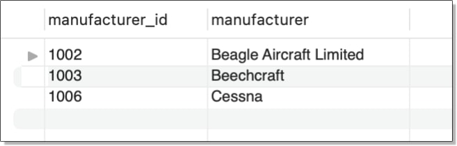
The column data returned by the subquery includes only those manufacturers that offer planes with piston engines (as reflected in the current data set). The IN operator determines whether the current manufacturer_id value is included in that list. If it is, that row is returned, as shown in the following figure.

As with many operations in MySQL, you can take different approaches to achieve the same results. For example, you can replace the IN operator with an equal comparison operator, followed by the ANY keyword, as shown in the following example:

SELECT manufacturer_id, manufacturer 
FROM manufacturers
WHERE manufacturer_id = ANY 
  (SELECT DISTINCT manufacturer_id FROM airplanes
    WHERE engine_type = 'piston');

You could have instead used another comparison operator, such as greater than (>) or lesser than (<) or even ALL instead of ANY. The statement returns the same results as the previous example. In fact, you can also achieve the same results by rewriting the entire statement as an inner join:

SELECT DISTINCT m.manufacturer_id, m.manufacturer
FROM manufacturers m INNER JOIN airplanes a
  ON m.manufacturer_id = a.manufacturer_id
WHERE a.engine_type = 'piston';

I’m not going to go into joins here, but as I mentioned earlier, joins can sometimes provide performance benefits over subqueries, so you should be familiar with how they work and how they differ from subqueries (a topic that could easily warrant its own article).

With that in mind, be aware that you can also use the NOT keyword with some operators to return different results. For example, the WHERE clause in the following SELECT statement uses the NOT IN operator ensure the current manufacturer_id value is not in the list of values returned by the subquery:

SELECT manufacturer_id, manufacturer 
FROM manufacturers
WHERE manufacturer_id NOT IN 
  (SELECT DISTINCT manufacturer_id FROM airplanes);

In this case, the subquery returns a distinct list of all manufacturer_id values in the airplanes table. The list is then compared to each manufacturer_id value in the manufacturers table, as specified by the outer query. If the value is not in the list, the search condition evaluates to true and the row is returned. In this way, you can determine which manufacturers are in the manufacturers table but are not in the airplanes table. The query results are shown in the following figure.

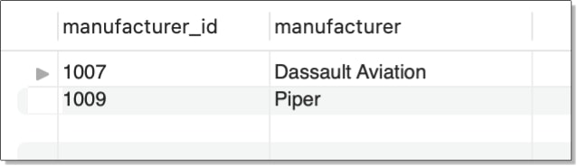
Be very careful when using NOT IN with your subqueries. If the subquery returns a NULL value, your WHERE expression will never evaluate to true.

Another operator you can use in the WHERE clause is EXISTS (and its counterpart NOT EXISTS). The EXISTS operator simply checks whether the subquery returns any rows. If it does, the search condition evaluates to true, otherwise it evaluates to false. For example, the following SELECT statement defines similar logic as the preceding example, except that it checks for which manufacturers are included in both tables:

SELECT manufacturer_id, manufacturer 
FROM manufacturers m
WHERE EXISTS
  (SELECT * FROM airplanes A
    WHERE a.manufacturer_id = m.manufacturer_id);

Notice that you need only specify the EXISTS operator followed by the subquery. If the subquery returns a row for the current manufacturer_id value, the search condition evaluates true and the outer query returns a row for that manufacturer. The following figure shows the results returned by the statement.

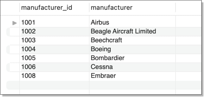
When working with column subqueries, it’s important to understand how to use comparison operators such as IN, NOT IN, ANY, ALL, and EXISTS. If you’re not familiar with them, be sure to refer to the MySQL documentation to learn more.

Using subqueries in the FROM clause

In addition to rows, columns, and scalar values, subqueries can also return tables, which are referred to as derived tables. Like other subqueries, a table subquery must be enclosed in parentheses. In addition, it must also be assigned an alias, similar to specifying a table alias when building correlated subqueries. For example, the following SELECT statement includes a table subquery named total_planes, which is included in the FROM clause of the outer statement:

SELECT ROUND(AVG(amount), 2) avg_amt
FROM 
  (SELECT manufacturer_id, COUNT(*) AS amount 
  FROM airplanes
  GROUP BY manufacturer_id) AS total_planes;

Notice that the outer statement does not specify a table other than the derived table returned by the subquery. The subquery itself groups the data in the airplanes table by the manufacturer_id values and then returns the ID and total number of planes in each group. The outer statement then finds the average number of planes across all groups. In this case, the statement returns a value of 5.00.

Now let’s look at another example of a table subquery. Although this next example is similar to the previous one in several ways, it includes something you have not seen yet, one subquery nested within another. In this case, I’ve nested a table subquery within another table subquery to group data based on custom categories and then find the average across those groups:

-- outer SELECT calculates average count across all categories
SELECT
  ROUND(AVG(amount), 2) AS avg_amt
FROM
  -- outer subquery aggregates categories and calculates count for each one
  (SELECT category, COUNT(*) amount 
  FROM 
    -- inner subquery categorizes planes based on parking area
    (SELECT CASE
      WHEN parking_area > 50000 THEN 'A'
      WHEN parking_area >= 20000 THEN 'B'
      WHEN parking_area >= 10000 THEN 'C'
      WHEN parking_area >= 5000 THEN 'D'
      WHEN parking_area >= 1000 THEN 'E'
      ELSE 'F'
    END AS category
    FROM airplanes) AS plane_size
  GROUP BY category
  ORDER BY category) AS plane_cnt;

The innermost subquery—the one with the CASE expression—assigns one of five category values (A, B, C, D, E, and F) to each range of parking area values. The subquery returns a derived table named plane_size, which contains a single column named category. The column contains a category value for each plane in the airplanes table.

The data from the plane_size table is then passed to the outer subquery. This subquery groups the plane_size data based on the category values and generates a second column named amount, which provides the total number of planes in each category. The outer subquery returns a derived table named plane_cnt. The outer statement then finds the average number of planes across all groups in the derived table, returning a value of 5.83.

Working with MySQL subqueries

Like many aspects of MySQL, the topic of subqueries is a much broader than what can be covered in a single article. To help you complete the picture, I recommend that you also check out the MySQL documentation on subqueries, which covers all aspects of how to use subqueries. In the meantime, you should have learned enough here to get a sense of how subqueries work and some of the ways you can use them in your SQL statements. Once you have a good foundation, you can start building more complex subqueries and use them in statements other than SELECT queries. Just be sure to keep performance in mind and consider alternative statement strategies, when necessary, especially if working with larger data sets.

 

The post Subqueries in MySQL appeared first on Simple Talk.

from Simple Talk https://ift.tt/PRWcA0Q
via

Backing Up MySQL Part 6: Physical vs. Logical Backups

Everyone who has ever backed up data using any kind of RDBMS knows a thing or two about backups. Backups are a central part of data integrity – especially nowadays, when data breaches are happening left and right. Properly tested backups are crucial to any company: once something happens to our data, they help us quickly get back on track. However, some of you may have heard about the differences between backups in database management systems – backups are also classified into a couple of forms unique to themselves. We’re talking about the physical and logical forms – these have their own advantages and downsides: let’s explore those and the differences between the two. This tutorial is geared towards MySQL, but we will also provide some advice that is not exclusive to MySQL.

What are Logical Backups?

Logical backups are backups of data consisting of statements that let the database recreate the data. Think of how you usually take backups within MySQL – no matter if you find yourself using the Export functionality within phpMyAdmin or using mysqldump to back up your most precious data, both of those measures have the same thing in common – they create statements that recreate data, creating logical backups as a result. And that’s exactly what defines logical backups – logical backups aim to recreate data by running SQL statements.

Sometimes though, developers might find themselves in waters where recreation of files is required.

What are Physical Backups?

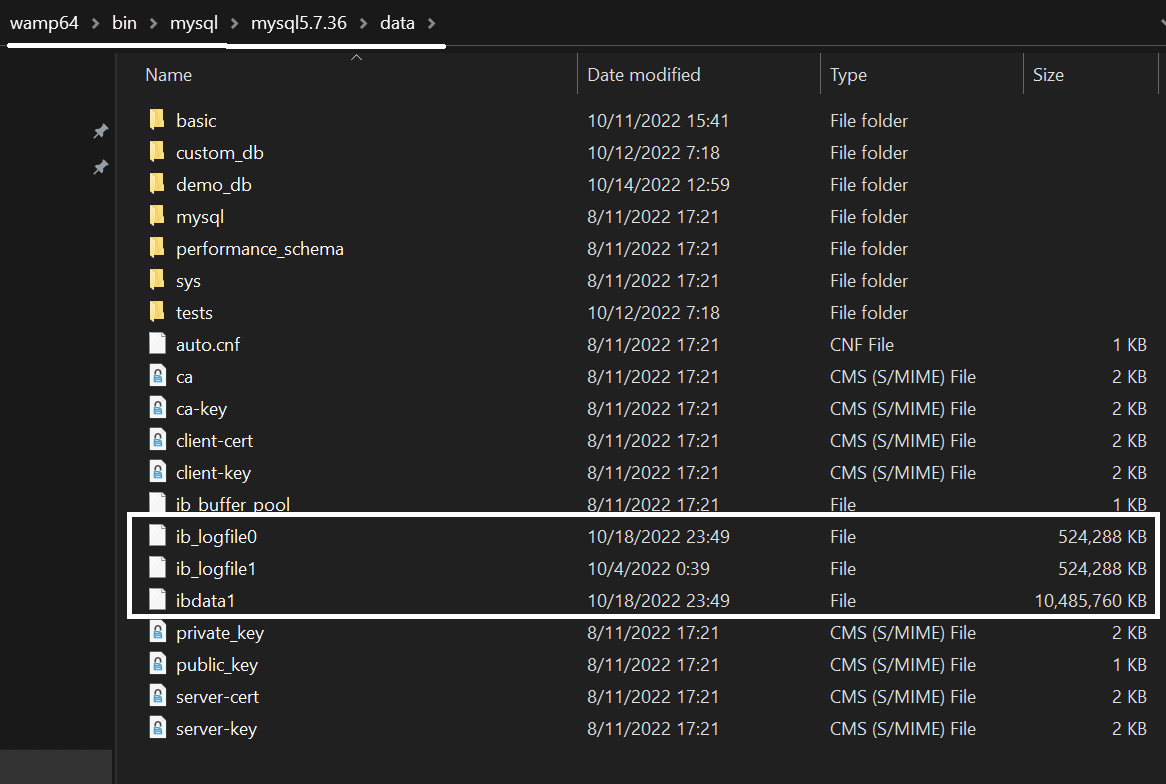
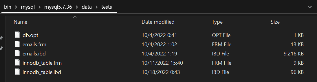
Physical backups, as you might’ve guessed, copy the “physical” data – files – that comprise a database. As far as MySQL is concerned, the physical backup of MySQL usually consists of a copy of the data directory found here (Windows-based example – in Linux, the directory would be /var/lib/mysql/mysql5.7.36/data):

Logical Backups in MySQL

Taking logical backups within MySQL is easier than you might’ve guessed – think of any part of MySQL that backs up statements to recreate data. Got one? You’ve got yourself a logical backup!

In MySQL, logical backups are taken by:

• The Export functionality in phpMyAdmin
• Using mysqldump
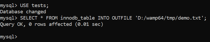
• Or using the SELECT [columns] INTO OUTFILE [path] statement in a specific database:

phpMyAdmin

Contrary to popular belief, the export functionality within phpMyAdmin can offer quite a lot of options to choose from. Users have a variety of options to choose from, including, but not limited to:

• The ability to choose whether to back up table structure, data, or both;
• The ability to choose the format of the backup;
• The option to can lock the tables while data is being written to them;
• The ability to export tables as separate files;
• The ability to compress the backup, skip tables larger than a specified value, etc.

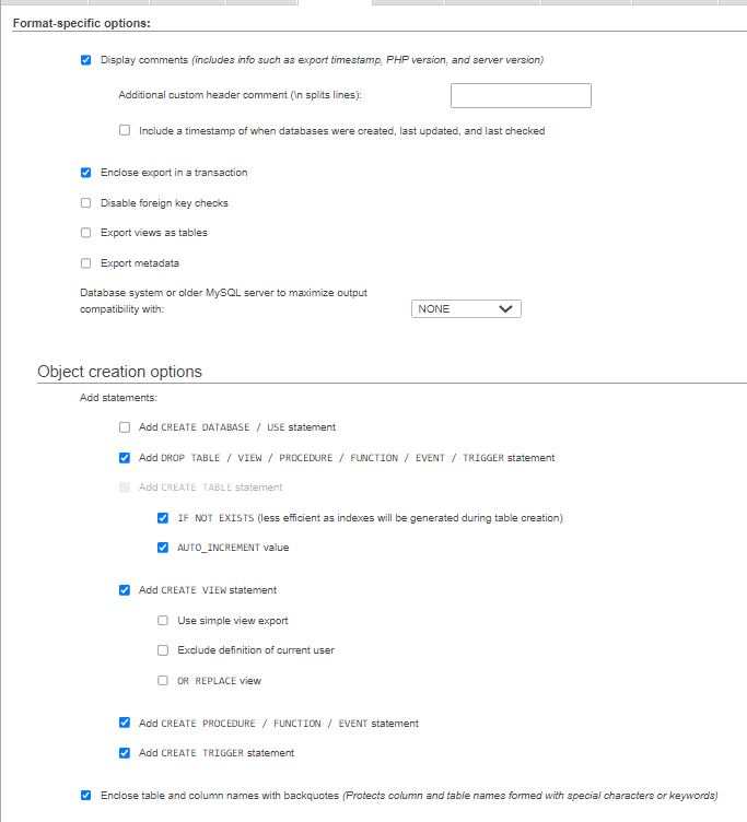
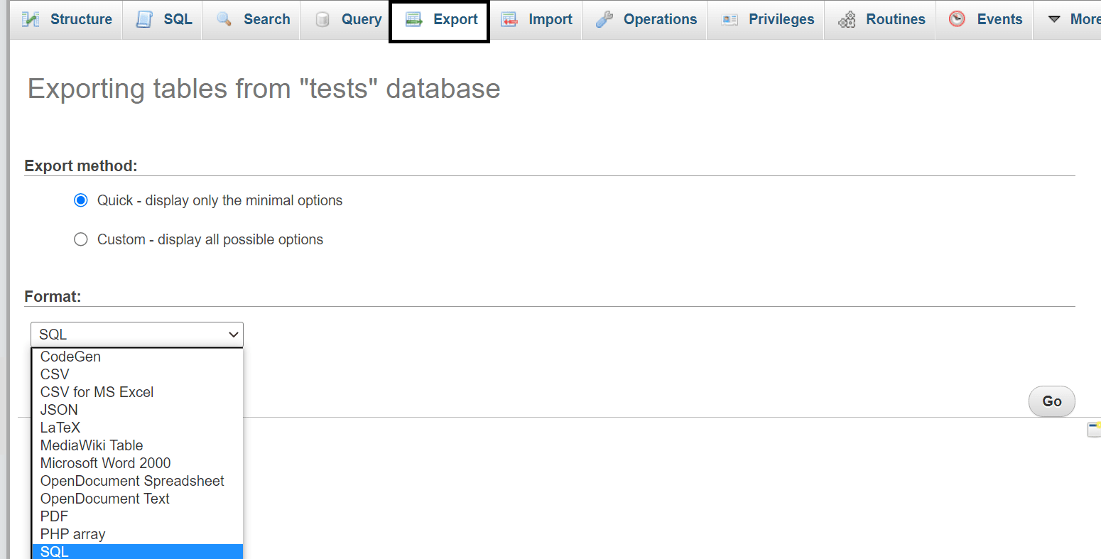
Some of the abilities of phpMyAdmin can be seen below:

Since phpMyAdmin is one of the most widely used tools within MySQL, it’s logical (see what we did there?) that it offers a lot of options for both junior developers and experienced DBAs alike (see example above.) phpMyAdmin isn’t anything fancy and it’s been here for decades – yet, its slick UI and rich feature set make it stand out from the crowd.

mysqldump

The next tool in the toolset of a MySQL DBA is, of course, mysqldump itself – the tool works much like the Export functionality within MySQL, just that it’s command line-based. For all of the nitty-gritty details, refer to the first blog of these series, but in a nutshell, mysqldump is once again blessed with an extremely rich set of features including, but not limited to:

• An ability to let backups continue being performed even if errors are encountered.
• An ability to only dump the schema within the tables.
• Only dump data matching a specific WHERE clause.

In order to use mysqldump, we need to be privileged enough to issue SELECT queries, and the syntax would look something similar to the following statement (to be issued before you log in to your database via the CLI on Windows or Linux):

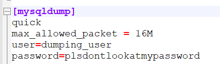
If you’re security minded, keep in mind that you can also prevent yourself from providing a username (-u) and the password (-p) by specifying it in the main configuration file of MySQL under the [mysqldump] heading like so (specify the user and password variables) – doing so will prevent anyone from seeing your username and password in the list of last issued commands in Linux:

For many people, phpMyAdmin and mysqldump provides enough of a grip into the world of backups – however, some might say the capabilities of the tools are a little lacking; those who venture into the world of big data might have to confirm the statement from experience – while both phpMyAdmin and mysqldump can offer powerful methods to back your data up in a fashion that is quicker than usual (LOCK TABLES provides developers with the ability to lock tables for a certain time until the backup is finished making its operations significantly quicker), both of those methods have a glaring flaw – the backups they create are riddled with INSERT statements.

There’s nothing “wrong” with INSERT statements per se, but their weakness is that they’re very ill-equipped to handle anything more than a couple million rows at a time: the core reason behind this is that INSERT statements come with a lot of overhead that MySQL has to consider – amongst other things, that includes parsing too. Imagine running 500,000 INSERT queries one after another where MySQL has to complete the following steps:

1. Start.
2. Check for permissions.
3. Open tables.
4. Initialize the query.
5. Acquire locks.
6. Do its work (run the query.)
7. Finish (“end”) the query.
8. Close tables.
9. Clean up.

Complete these steps. Now complete them again and repeat everything for additional 499,998 iterations. Does that sound quick? Sure, if we lock the tables, we might avoid the steps #3 and #8, but our queries will be slow nonetheless – there are a lot of things MySQL has to consider when running INSERT queries. There is a solution, though – we should also look into the LOAD DATA INFILE [path] INTO TABLE [table] query which is specifically designed for big data sets.

SELECT INTO OUTFILE & LOAD DATA INFILE

An alternative to INSERT that’s specifically designed for big data sets looks something like this:

LOAD DATA INFILE ‘/tmp/data.txt’ INTO TABLE demo_table [FIELDS TERMINATED BY|OPTIONALLY ENCLOSED BY] “|”;

That’s the LOAD DATA INFILE query, of course. It’s designed specifically for bulk data loading, and it’s capable of loading data in with “bells and whistles”:

• It’s able to skip certain lines or columns.
• It’s able to only load data into specific columns.
• It comes with significantly less overhead for parsing.

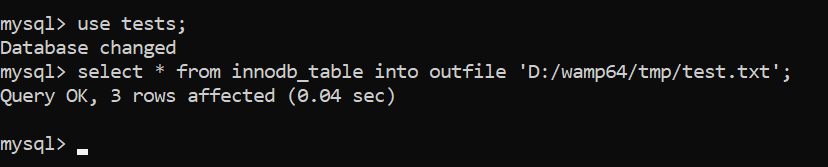
When LOAD DATA INFILE is in use, MySQL doesn’t perform as many operations as it does when INSERT INTO is in use, making operations significantly faster. To take a backup of your big data set use its brother – SELECT * INTO OUTFILE – like so:

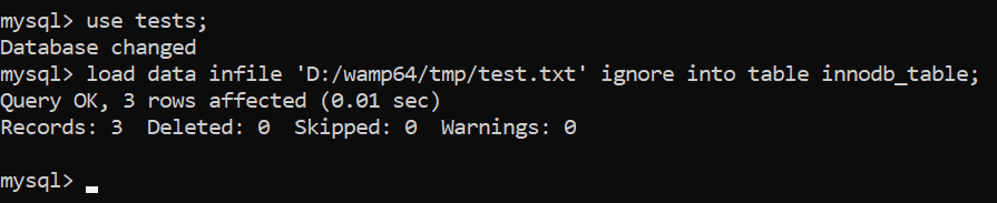
Then use LOAD DATA INFILE to load data back into your database (here we also use the IGNORE statement to ignore all potential errors – duplicate key issues, etc.):

Recap

• Backups taken by both phpMyAdmin and mysqldump can be simply re-imported into MySQL by using a simple query like so or via the phpMyAdmin interface (remove the -u and -p options if the username and password is specified in my.cnf):
  mysql -u root -p [database_name] < database_backup.sql
• To restore a backup taken using SELECT … INTO OUTFILE, use LOAD DATA INFILE.

However, while these three options comprise logical backups – the most frequently used form of backups in MySQL – and the process of taking them is quick, easy and straightforward, keep in mind that there’s also another way to accomplish your goals – people can also take backups in a physical form. Such backups copy files containing the data instead of recreating statements that build the data.

Physical Backups in MySQL

Physical backups offer the ability to copy files (physical data) instead of the statements that recreate it. To take a physical backup in MySQL:

1. Make sure MySQL is shut down (otherwise we’d be copying files that MySQL is still working with.)
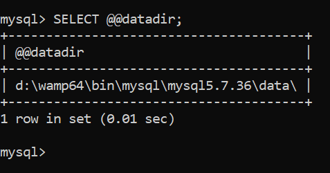
2. Head over to the data directory (entering SELECT @@datadir while logged in to your MySQL instance will help you see where it is):

1. Head over to the directory where you’ll store the physical backup, then create a directory inside of it using mkdir:
   mkdir [directory_name]
2. Copy the files named ibdata1 (the main tablespace file of InnoDB), ib_logfile0 and ib_logfile1 (undo and redo logs exclusive to InnoDB) to the directory you just created, then copy the data directory itself. Do note that if the data directory is big, copying operations will take some time.
3. You just took a physical backup!

If, for some reason, you find yourself using MyISAM (which is obsolete at the time of writing), taking physical backups of it is even easier – you just need to copy the data folder containing your databases, their data (.MYD files) and associated indexes (.MYI files.)

Physical backups can be useful when there’s a necessity to restore everything from a database from some media storage in one go, however, some might call the process of taking them a little tedious. To each their own though.

Recap

Physical backups copy the files that the data is based upon – to take a copy of them when using InnoDB, take a copy of the InnoDB tablespace (ibdata1) and the undo & redo logs (ib_logfile0 & ib_logfile1), then the data folder. To back up MyISAM, take a copy of all of the data and index files (.MYD and .MYI files) in the data folder.

Summary

MySQL offers everyone a couple of ways to back up data – while the most common option are logical backups that back up statements that recreate the data, indexes, partitions, and all related details, some might make use of physical backups where users copy the data files themselves: each option has its own upsides and downsides, so make sure to try both options out before your plan out your backup strategy. Familiarize yourself with all of the options, then make your own, physical or logical, decision.

We hope that this blog has been informational and that you’ve learned something new, and until next time!

The post Backing Up MySQL Part 6: Physical vs. Logical Backups appeared first on Simple Talk.

from Simple Talk https://ift.tt/TMdH0CE
via

Backing Up MySQL Part 5: Big Data

According to research made by Statista in 2022, the amount of data that is being worked with globally is expected to reach more than 180 zettabytes. Part of that is because more and more data is being introduced to the online world – but another part has its roots in software development. There are approximately 24.3 million software developers in the world (source: InApps), and with the number increasing every year, there‘s bound to be a lot of work with data.

The one thing that has always helped software developers work with data are databases – databases are not all made equal though. Some are said to be a fit for working with bigger data sets (MongoDB comes to mind), some are fit for timescale data (think TimescaleDB), some are a good fit for other use cases.

However, MySQL is MySQL – the RDBMS has been here for ages, and undeniably, it‘s here to stay. As with every database management system, MySQL has its upsides and downsides – one of the biggest notable downsides of MySQL is that many people think that it‘s not a fit for working with big data.

However, that’s not exactly true – MySQL is powering some of the biggest websites in the world from Facebook (for Facebook, MySQL is one of the main database management systems of choice as the social network stores almost all of the necessary data in it), to some of the biggest & fastest data breach search engines in the world letting people secure themselves from identity theft.

MySQL is a powerful, but a complex beast and in this blog, we will tell you how to back up big data sets within that beast.

The Infrastructure of MySQL

Before working with bigger data sets inside MySQL, you should familiarize yourself with its infrastructure. The most frequently used storage engine specific to MySQL is InnoDB and its counterpart XtraDB developed by Percona. Both InnoDB and XtraDB have a couple of properties unique to themselves:

1. The functionality of InnoDB is based on the InnoDB buffer pool – the buffer pool is an area used to cache the data and indexes when they are accessed. The bigger it is, the faster certain types of queries that are using the buffer pool or its data (SELECT, LOAD DATA INFILE) will complete.
2. InnoDB supports the ACID model guaranteeing data atomicity, consistency, transaction isolation, and durability. Note that even though InnoDB is known to offer support for ACID properties by default, it can also be made to exchange ACID for speed (and vice versa.)
3. InnoDB has a couple of acquaintances – while InnoDB data is stored in the ibdata1 file, InnoDB also has a couple of log files – ib_logfile0 and ib_logfile1 – that are used to store undo and redo logs. Undo logs contain information about undoing changes made by a specific transaction, while redo logs store information about how to re-do them (hence the names.) Both files can be found either in the /var/lib/mysql/mysql*.*.**/data directory if Linux is in use, or in the /bin/mysql/mysql*.*.**/data directory if you find yourself using Windows (*.*.** represents the MySQL version):
   
4. All of the settings relevant to InnoDB can be configured via the settings present in my.cnf.

Now as far as backups are concerned, we don‘t need to know much about the internals of InnoDB (or any other MySQL storage engine for that matter) because we can simply take them using mysqldump, mydumper, or through phpMyAdmin by heading over to the Export tab:

All of those tools will provide us with logical backups that can be used to restore data whenever we please, however, for those of us that work with bigger data sets, neither of those tools are an option – as INSERT statements contained in the backups derived from those tools usually come with a lot of overhead, developers frequently find themselves needing to dip their toes in other waters instead.

Backing Up Big Data

Logical Backups

In order to back up data sets that are bigger in size, developers need to keep a couple of things in mind:

1. First off, if a logical backup is being taken, we should avoid creating a backup filled with INSERT INTO statements – this article should provide you with a little more information what these are, but the main reason such statements are to be avoided is because such statements come with a lot of overhead that MySQL has to consider. In order to execute a single INSERT statement, MySQL has to check for permissions, open the necessary tables, initialize the query, acquire all locks that are needed for the query to execute, run the query, finish the work (let the query run until it’s finished), close tables and perform additional clean up operations. Of course, these might be relatively quick to complete in the grand scheme of things, but we need to consider that we would be working with hundreds of millions of rows at a time.
2. Working with big data sets would require a dedicated server, or at the very least, a VPS. This one is probably already out of the question (you’ve done your investigation into the hosting provider before choosing one, right?), but nonetheless, choosing the right server for our big data project is always a necessity.
3. How many databases are we backing up? How many tables are inside of those databases? Do all of those need to be backed up? You would be surprised how many times we can limit the amount of data that is being backed up by simply thinking ahead.
4. Did we work with bigger data sets before? Our experience in the past teaches us more lessons than we could imagine – however, if we didn’t have much experience beforehand, we can also just ask around – if our colleagues are well-versed in the field, the answers to most pressing questions shouldn’t be too far away.

Once the basics are covered and we’ve decided what we’re backing up, it’s time to move on. The best way to take a logical backup of a bigger data set is to use the LOAD DATA INFILE query – since the query comes with many of its own bells and whistles, it’s significantly faster than ordinary INSERT statements:

• MySQL needs little overhead to parse the query.
• Users can easily skip lines or columns.
• Users can easily specify the columns to load the data into at the end of the query.

It’s important to note that MySQL offers two ways to use LOAD DATA to load data into our infrastructure – LOAD DATA LOCAL is another query that users can use. The local option only works if we didn’t define the local-infile option to be 0 or if the local-infile option is defined within my.cnf underneath the [mysql] and [mysqld] headings. The LOAD DATA LOCAL query is widely considered to be insecure because the parsing of data happens on the server side – the local option:

• Invokes certain security functions of MySQL that must be followed.
• Changes the behavior of MySQL when searching for the file to import.
• In some cases (when dealing with errors, etc.), it has the same effect as IGNORE does.

The most important security considerations are explained here.

The main reason LOAD DATA INFILE works so well with bigger data sets though is because the files created with it only contain the data that is being backed up separated by a specific character (“:”, “|”, “,”, Tab, etc.) – MySQL can then load the data straight into a specific column without performing any additional operations and know where the set of data “ends” as well. A basic query looks like so:

LOAD DATA INFILE ‘file.ext’ INTO TABLE demo_table [options]; where:

• file.ext is a file bearing any extension other than SQL (.txt, .csv, etc.);
• demo_table defines the table that the data will be loaded into.
• After the file and the table are defined, we can choose to define certain options:
  • TERMINATED BY will make our columns end with a certain character (it can be useful when our file has a lot of records that are terminated by a character):
    LOAD DATA INFILE ‘file.ext’ INTO TABLE demo_table TERMINATED BY ‘|’;
  • CHARACTER SET will make MySQL use a specific character set when importing the data. This feature can be very important when loading in data that comes from a different geographical place than the existing data (e.g. if our data is from England, and we’re importing data from Korea, China, Russia, etc.) – it will help us avoid errors when importing such data sets – learn more about charsets here.
    LOAD DATA INFILE ‘file.ext’ INTO TABLE demo_table CHARACTER SET latin1;
  • PARTITION will make MySQL able to insert data into a specific partition – that’s very useful when working with bigger partitioned data sets – the partition can be specified like so (p1, p2, and p3 defines the partitions):
    LOAD DATA INFILE ‘file.ext’ INTO TABLE demo_table PARTITION p1, p2, p3;
  • IGNORE LINES|ROWS can be used to ignore certain lines or rows – this feature can be very useful when we want to ignore a certain amount of rows or lines when importing big data sets – perhaps we only want to import rows starting from the row #25527? (we can either ignore lines or rows):
    LOAD DATA INFILE ‘file.ext’ INTO TABLE demo_table IGNORE 25526 LINES|ROWS;

All of the options can be found at the MySQL documentation.

As far as backups of big data are concerned, the most popular options that are used are as follows:

1. TERMINATED BY
2. PARTITION
3. CHARACTER SET
4. IGNORE LINES|ROWS

Each of those options have their own upsides (see above) and when combined with an exceptionally large data set (think 100M rows and above), they make the LOAD DATA INFILE operation even more powerful than before.

To take a backup that can be restored by using the LOAD DATA INFILE statement on the other hand, we’d need to use the SELECT [columns] INTO OUTFILE statement:

SELECT * FROM demo_table INTO OUTFILE ‘backup.txt’ [options];

The options remain the same. That’s it!

Another consideration that is worth mentioning is the IGNORE keyword: the keyword will ignore all of the errors derived from the query: think not all entries having enough columns, some rows being wrongfully terminated (terminated with the wrong character), etc. – to make use of the keyword in LOAD DATA INFILE operations, specify it like so:

LOAD DATA INFILE ‘path/file.txt’ IGNORE INTO TABLE demo_table [options];

To make use of the keyword in SELECT ... INTO OUTFILE operations, make use of the keyword like so:

SELECT * INTO OUTFILE ‘demo.txt’ IGNORE FROM demo_table [options];

Contrary to popular belief, the IGNORE keyword has more use cases than we could think of – can you imagine how much time is saved by ignoring thousands or even millions of errors?

Physical Backups

As far as physical backups are concerned, backing up big data sets is not that different from backing fewer amount of rows – here’s what we have to consider:

1. We can either take a hot or cold backup (a hot backup is taken when a database is still running, while a cold backup is taken while the database is down.)
2. We need to consider whether we will use tools or take the backup manually (the tools that come to mind in this space include MySQL Enterprise Backup and others.)

If you decide to take a hot backup, most of the time you will be advised to use mysqlbackup (MySQL Enterprise Backup) as it provides good results with minimal downtime.

If we decide on a cold backup, the following steps should help:

1. Shut down MySQL.
2. Copy all of the files relevant to your storage engine of choice – if you’re using InnoDB, take a backup of ibdata1, ib_logfile0, and ib_logfile1 and store them somewhere safe (If you’re using MyISAM, simply take a backup of .MYD and .MYI files in your MySQL data directory and stop here.)
3. If you’re using InnoDB, take a copy of all of the tables in the data directory of MySQL (start from the /var/lib/mysql/bin/ directory if you find yourself using Linux – if you’re using Windows, follow the path given below):
   
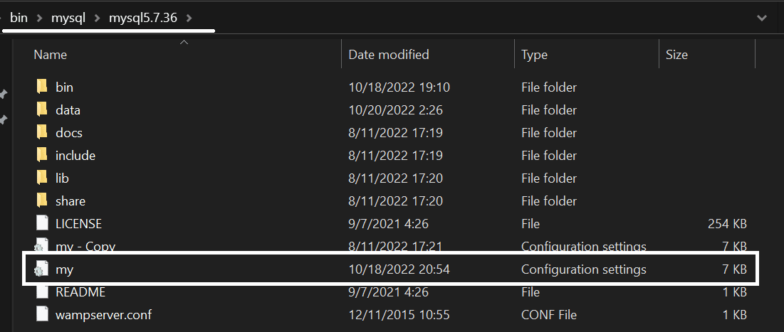
4. Finally, take a copy of my.cnf – the file can be found in /var/lib/bin/mysql/mysqlversion when using Linux – if you find yourself using Windows, the file is called my.ini and it can be found here (keep in mind that taking a copy of the file can be useful to review old settings as well):

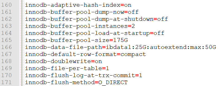
For those who are interested, the settings within the file will most likely look like so – if you want to, feel free to explore the file, then come back to this blog:

Anyhow, here’s why performing all of these things is a necessity:

1. Shutting down MySQL will ensure that nothing interferes with our backup operation.
2. The backup of ibdata1 will take a backup of all of the data existing in InnoDB, while backing up the ib_logfile0 and ib_logfile1 will back up the redo logs.
3. Taking a copy of the .frm and .ibd files is necessary because as of MySQL 5.7.8, only table metadata is stored in ibdata1 to prevent congestion – the actual table data is stored in the .frm and .ibd files (an .ibd file contains the data of the table, while an .frm file contains table metadata.)
4. Taking a copy of my.cnf (or my.ini if we find ourselves using Windows) is an absolute necessity as well because the file contains all of the settings relevant to all storage engines in MySQL. That means that even if we are using an obsolete storage engine like MyISAM and want to continue running the engine on the server that we’re loading the backup onto for some reason (MyISAM provides faster COUNT(*) operations because it stores the number of rows in the table metadata – InnoDB does not), we can.
5. Finally, make sure to store everything in a safe and accessible place – doing so allows us to recover data whenever we need to.

To restore a hot backup taken by using MySQL Enterprise Backup, once again refer to our blog, and to restore a cold physical backup taken by following the steps above, follow the steps below (the steps are specific to InnoDB):

1. While MySQL is still down, copy over your my.cnf file to your server and adjust the settings within the file to your liking.
2. Place the folders contained within the data folder when backing up back into the data directory.
3. Place the ibdata1 file and the log files back into the data directory of MySQL (see above for an example.)
4. Start MySQL.

To recover your MyISAM data, simply copy over the data folder to your server. No further action is necessary due to the fact that MyISAM doesn’t store additional data in files as InnoDB does.

To take and restore physical backups of InnoDB, we can also use PITR (Point-In-Time Recovery) – some say that the PITR method is significantly easier, but that depends on the person. Anyway, the MySQL manual should walk you through all of the necessary steps.

Summary

Backing up big data sets in MySQL is not the easiest thing to do – however, with knowledge centered around how the main storage engine (InnoDB) works internally and what queries we can run to make our backup process faster, we can overcome every obstacle in our way.

Of course, as with everything, there are certain nuances, so make sure to read all about them in the MySQL documentation chapters surrounding the necessary functions you need to employ – came back to this blog for more information about database functionality and backups within them, and until next time!

The post Backing Up MySQL Part 5: Big Data appeared first on Simple Talk.

from Simple Talk https://ift.tt/56bLHMR
via

Express.js or Next.js for your Backend Project

Backend projects create projects to execute code on a centralized server and then communicate results with a client. These kinds of projects are executed efficiently with Express.js, and the number of web developers who use this framework is increasing daily. Next.js, on the other hand, makes backend projects more interesting because you can use it alongside an existing backend as well as for frontend development.

Both Next.js and Express.js are good tools for development and production projects. 

Development and production are terms that every software developer should know. Development refers to the stage when you are still building and experimenting with your application on your machine. It is not yet open for end users to do anything beyond quality assurance testing. Production represents the stage when your application is available for the public – end users– to use. You must have fixed all glitches at this stage (or at least all that you can find!), and the application is ready for users to do the work the application is built for and expect that work to be persisted. 

It is essential to state here that Express.js and Next.js are both powerful tools for creating an enjoyable user interface. However, both tools have peculiarities to understand so in this article I will help you decide whether Express.js or Next.js is the best Javascript framework for your backend project.

This article will compare Express.js and Next.js and show which may be preferable for you when embarking on a backend project.

What is Express.js?

Express.js (also referred to as Express) is a node.js web application framework. It is an excellent backend web tool and was founded by TJ Holowaychuk who also is the sole developer of Apex software.  Express.js is layered on node.js which aids in managing servers. Node.js is a reliable javascript runtime that is efficient in creating server-side applications. Express.js became popular when it was used by top brands like Fox Sports, PayPal, Une and IBM. For more companies that use Express.js, check this article on the Express.js website.

Web developers can make the most of the features of Express.js because it stands out among other web application frameworks, one reason being that developing with it is faster. In addition to this, it offers a less stressful system of debugging. If you are a developer, I am sure you understand how stressful finding and removing bugs from software can be. This is especially true with backend software as errors do not always show up directly to the end user.

What is Express.js used for?

In the JavaScript/Node.js ecosystem, Express.js is used to create applications, API endpoints, routing systems, and frameworks.

A selection of the types of applications you can build with Express.js on the backend include

• Single Page Applications
• Real Time Collaboration Software
• Streaming Software
• Financial Technology(Fintech) Applications

In the following sections I will discuss how Express.js can be used to implement these types of solutions.

Single-Page Applications

Single-Page Applications (SPAs) are a modern approach to application development in which the entire application is routed into a single index page. Express.js is an excellent framework for creating an API that connects these SPA applications to server resources and consistently allows them to serve data. Examples of single page applications include Gmail, Google Maps, Airbnb, Netflix, Pinterest, PayPal, and many other. Companies are using SPAs to create a fluid, scalable experience that works similar to an application in a browser window.

Real-Time Collaboration Software

Collaboration tools make it easier for businesses to work and collaborate daily. With Express.js, you can easily develop collaborative and real-time networking applications.

For example, this framework is employed to build real-time applications like chat and dashboard applications. Express.js make it virtually effortless to integrate WebSocket into the framework.

Express.js handles the routing and middleware portions of the process, allowing developers to focus on the critical business logic of these real-time features when developing live collaborative tools, rather than the real-time itegrations.

Streaming Software

Streaming software is ubiquitous these days. Most people use one like Netflix, Disney+, etc. Streaming software is complex real-time application typically using many layers of data streams. To build such an app, you’ll need a solid framework that can efficiently handle asynchronous data streams. Express.js It’s an excellent framework for developing and deploying enterprise-grade, scalable streaming applications.

Financial Technology (Fintech) Applications

Fintech refers to computer programs and other forms of technology that support or enable banking and financial services. Building a fintech application to support customers anywhere from any device is a continuing industry trend, and Express.js is one of the best frameworks for developing highly scalable fintech application

If your plan is to develop and deploy a fintech application with a high user and transaction volume, it may interest you to know that you’ll be joining companies like Paypal and Capital One in using Express.js.

What is Next.js?

Next.js is a React-based open-source web development framework. It was brought about by Vercel, which was formerly known as Zeit. It allows us to add functions – like server-side rendering and static web generations – to React based apps. In addition to this, it extends React to provide additional features that are extremely useful in production, such as caching, which improves response times and decreases the number of requests to external services.

Next.js is used in web development to create fast web apps. You can create a React app that uses server-side rendering to store content on the server in advance. End-users can easily interact with the HTML page and a user-friendly interactive website or app.

What is Next.js used for?

Next.js has handled quite a lot of problems in frontend for years now making big and popular companies to rely on it. It’s mostly known to help developers create performant web applications and speedy static websites. Below highlights some of the things that the framework is used for the following usage types, amongst others.

• Server-side rendering
• Static Websites
• Routers
• Web Software
• Code Splitting

In the following sections I will discuss how Next.js can help with these sorts of utilizations.

Server-side rendering

By default, Next.js performs server-side rendering. This optimizes your app for search engines. You can also use any middleware like express.js or Hapi.js, as well as any database like MongoDB or MySQL.

Static websites

By employing a static generation tool such as Next.js, you can serve a full page of content on the first load. Next.js’s static site generator provides good speed without sacrificing the quality.

Routers

A router is a mechanism that lets you determine what occurs when a user goes to a certain webpage. For more details, see this page on the Next.js website. This is yet another fantastic feature of Next.js.

When you make use of the create-react-app command, you must usually install react-router and configure it but Next.js includes its own routers with no configuration. The routers do not require any additional configuration. Simply place your page in the pages folder, and Next.js will handle all routing configuration.

Web software

Because Next.js possesses features such as the TypeScript support which helps to avoid and catch errors in the development phase, it is suitable for building large-scale and complex software. Next.js includes a robust debugging feature, which allows developers to debug their code by generating friendly error messages.

Authenticating statically generated pages permits Next.js to automatically determine that a page is static if no blocking data requirements exist. This allows Next.js to support different authentication patterns. Next.js can be used to create a client-friendly interactive user interface.

Code splitting

It is true that code splitting, also referred to as lazy loading, enhances the user experience of your application. In some applications, it’s possible that a page may take some time to load. If the loading time is long, the visitor may dismiss your app because they are not sure whether the application has failed or not.

To avoid this, a trick is used to show the visitor that the page is loading, such as displaying a spinner. Doing this allows you to deal with and control slow loading by only loading part of the JavaScript in your page quickly, and loading the rest while the user waits, confident that the site has not frozen up.

Next.js includes methods for splitting code that makes it easy to dynamic loading of pages.

Edges and Drawbacks

In this section, I will provide you with a set of positives and negatives for both Express.js and Next.js. This will help you to decide which of the libraries in this article is best in certain situations.

Edges of Express.js 

This section will cover a few aspects of Express.js that makes these JavaScript tools great for back-end development.

• It supports JavaScript, making it simple to learn. In addition to that, Express.js is also widely available and has a big community. 
• It offers a straightforward route for client requests.
• Express.js includes middleware that handles decision-making. You can define an error handling in the middleware as well.
• Express.js provides developers with convenience, flexibility, and efficiency.
• Asynchronous APIs are used.
• Express.js is compatible with any database. Databases like MongoDB, Redis, and MySQL are straightforward to connect to.
• It is simple to integrate with various template engines such as Jade, Vash, and EJS.
• It’s simple to serve static files and app resources.

Drawbacks of Express.js 

Express.js exercises a lot of benefits in web development but there are also drawbacks that comes with working with this tool. In this section I will list some of them.

• The middleware system provided by Express.js encounters a number of client request issues.
• There could be issues with asynchronous callbacks. For more information on such callback, visit this page.
• Developers who are familiar with other software languages may find Node.js’ event-driven nature difficult to grasp.
• Organization of code in Express.js projects can be complex.
• Express.js security can have security vulnerabilities that need frequent patching. For more details, visit this webpage.
• Its error messages are frequently ineffective, making it hard to debug at times.

Edges of Next.js 

Comparing Next.js with its counterparts, you’ll come across plenty of benefits and this section will highlight some of these benefits.

• The delivery of the complete webpage is ensured by static site generation.
• When developing Next.js projects, it allows for simple deployment. All you do is link up your account to GitHub and transfer your Next.js repositories. 
• It allows for simple page navigation. The Next.js router enables client-side route transitions between pages.
• API Routes allows you to use multiple HTTP actions for the identical address in the same file.
• Next.js includes TypeScript out of the box, making builds easier.
• The number of developers is increasing as the popularity of Next.js grows. As a result, it may be easier to find a company or freelancer to make any necessary changes.
• Security of data is reasonably easy to ensure using Next.js.
• It makes creating an outstanding user experience (UX) easy.

Drawbacks of Next.js 

Some features of Next.js might come up as a disadvantage when relating it to how it affects you, relating to a particular situation, time or project and this section will shed more light on those cons.

• Cost of flexibility is somewhat expensive. This is because Next.js does not include many installed front pages, so you must create the entire front-end layer from scratch.
• Development and management are worth considering.  Say you want to use Next.js to build an online store but don’t have an in-house development team, you may need to hire someone to handle the development and management subsequently.
• Because there is no built-in state manager, you will need to use Redux, MobX, or something similar.
• In comparison to Gatsby.js, there are fewer plug-ins available.
• Because Next. js supports static website development, the amount of time it takes do build software packages with many pages could be quite lengthy.

Key elements Comparison

In this table, I will show a list of key elements of a JavaScript libraries, and how Express.js and Next.js fit these elements.

Key elements	Express.js	Next.js
Data fetching	Doesn’t let Express.js deliver a response from server-side to an EJS template in client’s side	Next.js data fetching enables you to deliver your content in a variety of ways, based on the use case of your application.
Server use	Can be used both on the client-side and the server-side	Used for building server-side rendering applications
Plug-in and ecosystem	The Express Gateway plugin includes entities and supports event subscription.	Next.js makes use of existing powerful tools such as Webpack, Babel, and Uglify, and presents them to the end user in a stunningly simple interface.
Static generation	Deferred static generation.  Developers can choose to postpone the creation of specific pages until the first time a user requests them.	Incremental static generation. After you’ve built your site, you can use Next.js to create or update static pages.
Scalability	When developing a large-scale web application, it handles user API calls efficiently and requires little to no extra configuration.	Next, js makes it simple to scale multiple pages because it allows you to choose whether to render each page on the client, the server, or both.
Speed	a Node. js backend framework with minimalist and fast tools and functions for developing scalable backend applications	Because of the static destinations and server-side rendering, it is extremely fast.
SEO	It is beneficial for SEO as it offers crawlers from search engines with a fully rendered homepage, making their work easier.	Next.js is a fundamental tool for achieving impressive SEO performance.

Express.js Vs Next.js: Is either truly better?

There are numerous JavaScript packages available for use in your project but determining which one is best for you can be difficult. Many developers use Express.js because it is simple to learn and rapidly growing. Next.js is also popular because of its ease of use and performance advantages.

Next.js is smart enough to only load the Java and CSS required for each document. This results in much quicker page loading times because the user’s browser isn’t required to install JavaScript and CSS that aren’t required for the page where the user is viewing.

Express.js enables the routing of web applications utilizing multiple URL and HTTP methods. It enables an Express JS designer to handle a large number of orders and quickly generate responses for specific URLs. This enhances the user experience while also allowing the apps to scale.

These two are great tools to use for the project but the question of which is better lies in what exactly the nature of your project is. One is a specialized backend tool while the other is a full stack tool which can be used for both frontend and backend.

The post Express.js or Next.js for your Backend Project appeared first on Simple Talk.

from Simple Talk https://ift.tt/IbwU2C9
via

Backing up MySQL Part 4: mydumper

There are many tools we can use to back up our MySQL databases. Some are well-known and used by the best technology companies out there (mysqldump comes to mind), and some are a little less famous, but still have their place in the MySQL world. Enter mydumper – the tool is built by the engineering team over at Percona and it‘s supposedly created to address performance issues caused by mysqldump.

Prerequisites and Installation

mydumper is a tool that lets people take logical backups of their MySQL databases. The tool is built according to the best MySQL practices, it‘s being actively maintained, and works on all flavors of MySQL, including Percona Server and MariaDB. Note that the tool is not built-in to MySQL – to use it, one needs to install the development versions of MySQL or any of its flavors, install a couple of development tools, and install the development versions of GLib, ZLib, PCRE, and ZSTD – once all of these libraries are installed, we should follow the instructions for installation that are available here.

All of these libraries accomplish specific goals – GLib is a bundle of libraries, ZLib is used to compress data, PCRE stands for „Perl-Compatible Regular Expressions“, and ZSTD – otherwise known as ZStandard – is a compression algorithm developed by Facebook.

The installation of mydumper will provide us with:

• The ability to export and import data using multiple threads in parallel, sort of like mysqlpump does.
• The ability to use regex expressions when exporting data.
• Easily manageable output – all tables will be backed up into separate files exclusive to them, data and metadata will be separated, etc.

Using mydumper

Once mydumper is installed, we can start playing with the tool. Even though there are multiple advanced features provided by the tool, the syntax isn‘t rocket science and looks like the following:

mydumper [options]

That‘s it, really. Well, users will still need to specify the host (--host), user (--user), and password (--password) to work with, but other than that, only the options remain. The output that is received will, of course, vary and depend directly on the options that are specified, so let‘s look into them as well:

• Users can specify the --database option to provide mydumper with the database to work with (dump data from.) Alternatively, the --B option can also be specified.
• The --tables option, or its shortened version --T, will let users specify a comma-delimited list of tables to take a copy of.
• The databases and tables that are being dumped need to have an output directory that can be specified by appending --outputdir or --o (the directory must be writable.)
• Users can also split INSERT statements into smaller size by using --statement-size (or --s.) Note that the size of INSERT statements are to be specified in bytes (default size – 1,000,000 bytes.)
• mydumper allows its users to specify which storage engines to ignore (i.e. mydumper will not back up tables built on this specific storage engine) by using --ignore-engines or --i.
• The --regex or --r option will let users specify databases and tables using regex in the format of „database.table.“ Something like this should do:
  mydumper --regex „(^demo_db\.demo_database$)“
• To specify the number of threads mydumper is able to use (the default number of allocated threads is 4), consider the --threads or --t option.
• mydumper is also able to automatically send long-running queries to the timeout realm or kill long-running queries: that can be done by either specifying the --long-query-guard or --kill-long-queries parameters (or their shorter counterparts which are --l and --k respectively.)

The options specified above should tell you a little about just how powerful mydumper can be when used properly – however, do note that other options can be used as well – mydumper also comes with a brother called myloader which is essentially a backup tool that restores data generated by mydumper from a directory specified by the user. To use myloader, invoke it like so:

myloader --directory=[directory] [--overwrite_tables] --user=your_user

The --directory option takes the directory inside of which the backup created by mydumper is being stored, and the overwrite-tables option can also be invoked to overwrite all existing tables.

Make sure to read up on the docs surrounding the two tools here and follow Percona’s blog to learn more about the tools they develop – explore the Databases part of SimpleTalk to learn more about the functionality of all kinds of databases (our blog is not limited to MySQL!) and how they impact the behavior of applications, and we’ll see you in the next one.

The post Backing up MySQL Part 4: mydumper appeared first on Simple Talk.

from Simple Talk https://ift.tt/oWGdpUs
via