Tuesday, June 6, 2023

Power BI Connections Management

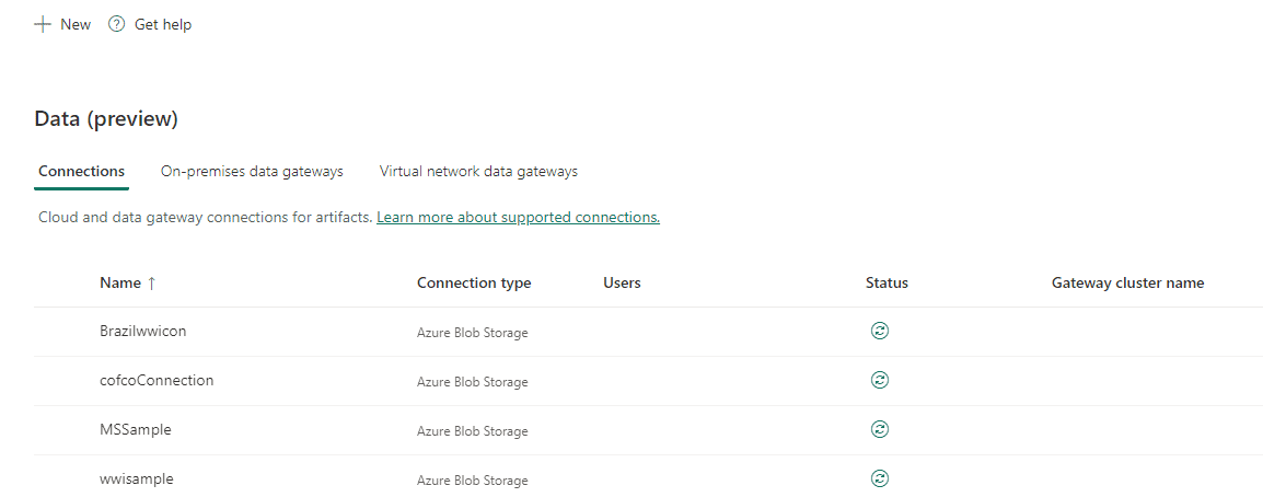
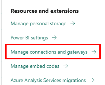
Some time between January and now, a new preview feature was included in Power BI Portal. It’s a new Manage Connections and Gateway window, still in preview. We can access this option on the Settings button.

Interface gráfica do usuário, Texto, Aplicativo Descrição gerada automaticamente

In the past, the connections were related to on-premises data gateways. For each gateway we could create many connections and manage who would be the users with permissions to re-use these connections.

This is a separation of responsibilities: A Power BI Administrator, or gateway administrator, can be the responsible to create and manage the connections, while Power BI developers can use the connections without knowing the details about the connectivity.

The cloud brought the need of the Virtual network data gateways, which I explained in another article. The connections can be linked to an on-premises data gateway, a VNet data gateway or can also be a direct connection to a cloud resource.

Considering this evolution, the new Connections Management window allow us to manage the connections by themselves, independent of the gateways.

Interface gráfica do usuário, Texto Descrição gerada automaticamente

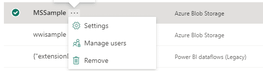
Each connection has an action button which allow us to manage the access to the connection (Manage Users), change the connection configuration (Settings) or remove the connection.

Interface gráfica do usuário, Aplicativo Descrição gerada automaticamente

Interface gráfica do usuário, Texto, Aplicativo, Email Descrição gerada automaticamente

Imagine creating 30 reports over the same connection. If you need to move the data source to a new place, you can reconfigure the connection one single time on the portal and all the reports will access the data from the new location.

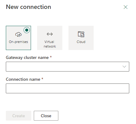
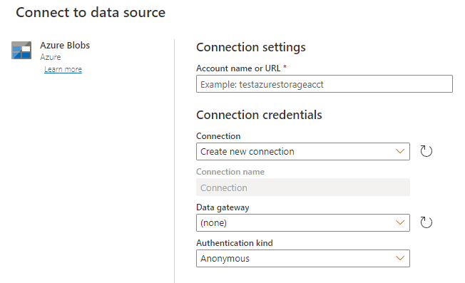
If we click the button New we can create a new connection. We can choose if the connection will be linked with an on-premises data gateway, a VNET Gateway or if it will be a connection directly to a cloud resource.

Interface gráfica do usuário, Aplicativo Descrição gerada automaticamente

Limitations of the Preview

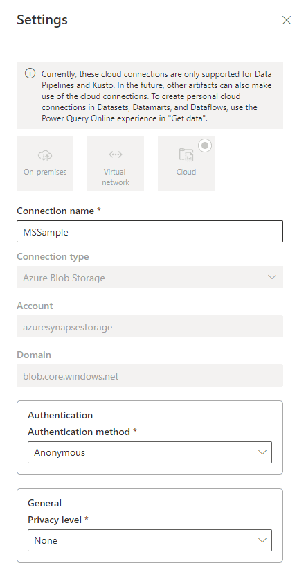
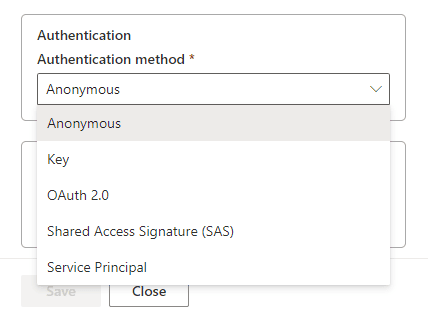
The connection configuration is limited at the moment: We can’t change the connection location, such as the address of the storage account, but we can change the authentication.

Interface gráfica do usuário, Texto, Aplicativo, chat ou mensagem de texto Descrição gerada automaticamente

We can use existing connections or create new ones in Microsoft Fabric. In Datamarts or Dataflows we can only create new connections, but not use existing ones. On the other hand, in Power BI Desktop we can’t create or use the connections at the moment.

Interface gráfica do usuário, Texto, Aplicativo Descrição gerada automaticamente

Conclusion

This feature is still limited, but it’s an important backbone service in Microsoft Fabric/Power BI environment which is related with many more resources in the entire Microsoft Fabric ecosystem.

The post Power BI Connections Management appeared first on Simple Talk.


from Simple Talk https://ift.tt/0aBfY8G
via

Monday, June 5, 2023

Why Test-Driven Development? (Part 1)

Software development is a very tough discipline. Robert Martin (better known as Uncle Bob) holds that software development is the toughest discipline because never before in human history was there an expectation to deal with such insane levels of details. Software development is so tough that it even created the movement called Extreme Programming (XP). We’re talking extreme levels of focus and hard work needed to produce quality software.

Since the core activity in software development is the activity of programming, what is the main challenge we’re faced with when attempting to program computers? Whenever we sit down to write some code, we are faced with two equally demanding challenges:

  1. We are focused on writing the code that will behave as expected.
  2. We are focused on writing the code that will be well structured.

It turns out that holding both expectations in our head at the same time tends to produce a lot of confusion. Trying to focus on two things at the same time is often a recipe for producing substandard material.

Is there a way to fix this impasse? Yes, there is a way – it was proposed by Kent Beck in the 1990s with his formulation of the Extreme Programming discipline. Kent proposed a different approach to writing programs by segregating the above two activities. This way of writing programs consists of first focusing on the activities that will produce code that behaves as expected. During this first phase, we neglect to focus on the quality of the code structure. In other words, we just write the code that comes easy to us. Meaning, it’s okay during this phase to break many rules and produce code that will make many professionals cringe and frown upon. That first pass of writing code (the first draft) is sloppy and messy; and that’s okay. We are asked to give ourselves permission to be sloppy at this juncture. Our aim at this point is single-minded – create code that will behave as expected.

And now for the crucial question: how do we know that the sloppy code we just wrote behaves as intended? We could manually verify the behaviour of the newly created code. But that would be very wasteful. Hey, here’s an idea – since we are very good at automating processes, why don’t we investigate automating our own development process? Instead of doing tedious, repeatable chores manually, why don’t we offload those chores to the machines?

What repeatable manual chores am I referring to here? I’m mostly thinking about the following scenario: we make a diff (a change) to the source code with the intention to get it to produce some desired behavior. We save those changes, and then embark on performing the following manual steps:

  1. Compile the code
  2. Build the app
  3. Configure the app
  4. Run the app
  5. Navigate to the login page on the app
  6. Log in with special credentials that simulate a specific user role
  7. Navigate the app to reach the section that is affected by the code change
  8. Enter some test data
  9. Examine the resulting output
  10. Log out and log in again with different credentials that simulate different user role
  11. Repeat steps from 7 to 9

Whew! That’s a lot of manual heavy lifting. Why are we doing things in such a pedestrian way? All the above steps can be easily automated. Saves not only time but also spares us from ‘fat fingers’ mistakes.

So, how do we automate the above chores? Simple – we write some code. But wait a minute – didn’t we just say that writing code is super tough because we are striving to satisfy two incompatible expectations (i.e., the expectation that the code behaves to our satisfaction and the expectation that the code is well structured). Well, in this case, the code we write to automate development chores is a different breed of code. Unlike the implementation/production/shipping code, which must be well-designed and properly structured, the code we write to automate our development activities need not be that fancy.

Rules for automating behavioral expectations

There is an adage in the software development profession: “Functionality is an asset; code is a liability.” That means we want to implement certain functionality, and if we can do it without having to write any code, that would be the most desirable outcome. However, oftentimes it is not possible to implement new functionality without writing some code, so a compromise seems unavoidable.

Functionality is what we call system behavior. Once implemented, the system behaves in certain automated fashion. While developing the system, we strive to make the system behave in the expected way(s).

To keep expectations about behavior separated from expectations about the code structure, we must write the expectation first. Let’s illustrate with a simple example. Suppose we are developing a tip calculator and we are expecting it to calculate tip percentages correctly. We can say “given an order total of $100.00, when the service was good, add $15.00 to the total to produce the grand total of $115.00”. That expectation stipulates that the system will calculate a 15% tip for a good service.

Okay, but how do we automate that expectation? We do it by writing a test. The test will first arrange for the preconditions by declaring the order total to be $100.00 and the service level to be ‘good’. The test will then envision that there is a system in place and that the test will be its first client. The test (i.e., the client) will notify the system saying, “here is the order total of $100.00 and the service was good; please calculate the tip and add it to the order total”.

To many software developers, this approach feels a bit odd, a bit backwards. Why are we spending time imagining how we could be interacting with an imaginary system? Isn’t it smarter to first build a system, and only then attempt to interact with it?

The reason we are envisioning how will the client’s interaction go with a not-yet-created system lies in our desire to keep our options open. We prefer to remain flexible. If we were to wait until the system gets built, we’d be coerced into having no choice but to interact with it in ways that may not make much sense to us, the client. The ease of understanding the system and the usability of the system are important aspects of the system design, which is why we are pursuing this train of thought.

So, by following this open-ended approach, we find ourselves in a very flexible position: we can envision any type of interaction with the nascent “tip calculator” system. We could call it directly and synchronously (i.e., blocking); we could try calling it asynchronously; we could even attempt to interact with it by publishing messages and letting the system subscribe to our publishing channel and consume our messages. Sky is the limit.

Once we formulate our first stab at how we would like the client to interact with the system, we can pretend that the interaction happened. The only thing left to do is to verify if the system behaved the way we expect it to behave. In this case, we are expecting the system to behave by returning $115.00 as the order grand total.

Now, in practical terms, this arrangement means that the expected system behaviour will not happen. We can try to run this half-baked test, and it will fail, of course. It cannot succeed for the simple reason that the system it is supposed to interact with does not exist yet.

But this failure is a good thing. It lets us know that our expectation hasn’t been met, and it gives us the impetus to keep going in the attempt to develop a system that satisfies our expectation.

From this little exercise, the most important thing is to focus 100% on our expectation regarding the system behavior. We need not waste any time pondering the implementation of the expected behavior. In other words, we are focused on formulating what is the system supposed to be doing, not on how the system is supposed to be doing it.

Separating the what from the how (separating the intention from the implementation) is a very powerful practice. It lets us focus on one thing at a time, which increases our chances of delivering quality work. Divide and rule is a maxim that is pretty much applicable to all situations.

The next thing to notice in the above exercise is that we are not formulating any conditional logic. The expectation, the test we have laid out above, is proceeding in a straight line. From arranging the preconditions (i.e., “given the order total is $100.00 and the service was good”), to triggering the system behaviour (i.e., sending the message to the yet-to-be-built system), to asserting the produced results (i.e., did the system return $115.00 grand total?). The last part is often referred to as post-condition (or, simply, assertion).

Pay close attention to how nowhere in the flow of the above test do we expect the code to make any branching decisions (in the form of “if this condition, then do that, otherwise do the other thing”). This ground rule is super important. It can be formulated as “never add any conditional logic to your tests!”

Of course, a testing framework itself possesses that branching logic, in the form of “if the expectation has been met, the test passes, otherwise the test fails”. Such branching logic is baked into the assertion statement offered by the testing framework; however, we don’t need to add any further logic to it; it is offered to us for free.

To summarize, two ground rules when automating behavioral expectations are:

  1. Envision what needs to be done, not how it will get done
  2. Avoid implementing any conditional (i.e., branching) logic in the test

How to work on meeting the expectation?

Now that we have crafted the shell of our expectation, how do we fulfill that expectation? In a more technical parlance, how do we make the failing test pass?

The recommended way to do that is to focus on two things:

1. Taking only small steps

2. Taking ordered small steps

The small-steps approach is another unusual aspect of this discipline. Professional software developers sometimes tend to view that approach as being suitable for novices, who are still learning the ropes. Then, once the ramping up process is done, novices graduate to intermediate/senior level and at that point they should dispose of the sheepish small steps and take the coding challenges in bigger strides.

That, however, is not the Test-Driven Development way. In TDD, we really cherish small steps. And by small steps I’d insist we mean micro-steps. Or one micro-step at a time.

Before we take a closer look into why micro-steps are so desirable, let’s have a look at what is meant by a micro-step. The first thing to ask always is: what is the smallest step we can do now? Usually, the smallest step is the simplest step. But that’s not always the case.

In this case, however, the smallest step we could possibly take would be crafting a skeleton of the system we intend to endow with expected behaviour. It could be a module, or a class, or some other construct containing executable code that could be triggered. Usually, such skeleton system can accept some input values and then return some output values.

So, we take our first small step by crafting a class or a module. That class/module can contain a simple function or a method that accepts arguments, or input parameters. For example, it can accept the order total and the service level parameters.

OK, but now that we have a simple system that accepts those values, how can we make that system behave? How can we make it return the expected value (in our case, we’re expecting it to return $115.00). We take the next simplest possible step – we return the hardcoded value. The body of the method remains empty, save for the simple statement:

return 115.00;

And with that simple change, we now have built the system that behaves as expected – it accepts the order total of $100.00 and the service level labeled as ‘good’, and then functions (i.e., behaves) by returning the $115.00 value. In effect, this test now passes! The expectation has been met. We’re done here.

Or are we?

More complex behavior

If every order total was $100.00 and if every service level was ‘good’, we wouldn’t have the need for developing an automated tip calculator app. What happens when, to keep things extremely simple, the order total is still $100.00 but the service level is ‘great’?

In that case, our expectation is that the system should add $20.00 to the order total, producing a grand total of $120.00. We can now write another test that formulates such expectation. When we run that test, it will fail. Why? Because it will send the order total of $100.00 and the service level ‘great’ to the tip calculator, but it will receive back the actual value of $115.00. And because it was expecting the actual value to be $120.00 in case of a great service, the assertion will fail.

How do we make the second test pass? The only way to make it pass is by replacing the hardcoded return value with some processing logic. The processing logic will have to make calculating decisions based on the type of the service. If the service was ‘good’, add 15% to the order total, if the service was great, add 20% to the order total. Both tests now pass.

What happens when we expect the system to calculate the tip for excellent service? We formulate another expectation. We create a new test that expects the actual grand total to be $125.00 given the order total of $100.00 and service level ‘excellent’.

Of course, this new test will fail (as it should). It fails because the system doesn’t know what to return when the service level is ‘excellent’. So, we need to modify our processing code to make it recognize the service level ‘excellent’ and then calculate the appropriate tip and add it to the order total (by applying 25% on the order total).

As should already be obvious from this exercise, we are growing the capabilities of our system in a very gradual, piecemeal fashion. And each step of the way is marked by a failing test that then passes once we make modifications to our shipping code.

It is also worth noting that our progression moves from very concrete code (as in hardcoded value) toward more abstract code (replacing hardcoded value with actual calculations that are performed on demand). We will see that TDD is a discipline that keeps egging us, little by little, away from more concrete code toward more abstract, more generic code.

For now, we have illustrated only one side of the Test-Driven Development process. We have accomplished the first challenge: making the code behave as expected. A bigger, more important side of this process – creating well-structured code — will be discussed in the next article.

Conclusion

The above-described approach to developing software will probably look ridiculous to developers who have never tried it. I know it looked not only ridiculous, but also very stupid to me when I first encountered it back in 2002. I could not believe why would anyone waste time writing more code than is necessary? Why write those executable expectations/tests when all we’re really asked to deliver is the shipping code? Obviously, no customer will ever agree to pay for those tests. Isn’t it logical then to avoid wasting time writing those tests?

Of course, even back then we all agreed that having regression tests is necessary. But those regression tests were to be written after we finish writing the shipping code, not before. Also, traditionally regression tests were the jurisdiction of the testers, or QA, not something software developers were expected to produce.

When it was explained to me that writing the test before we write the code is helping with the code quality, that didn’t make any sense to me either. I was confused – so, if we don’t think developers are capable of writing quality code without tests (which are supposed to drive the code quality), what makes us think that those same developers are suddenly capable of writing quality code in tests? Isn’t that approach just pulling the wool over our eyes? Tests are also code, and if we are doubtful that developers can write quality shipping code, why are we not doubtful that they can write quality test code?

We will clarify that dilemma in the following article. Still, for now, we should review one important aspect of the example we’ve examined so far. By following the simplest TDD practice, we were able to implement tip calculator functionality without ever resorting to any manual steps. None of the 11 steps exposed in the introduction had to be executed. From that, we see that TDD offers full software development process automation.

When making changes to our code, we never have to manually compile, configure, run, log in, navigate, and type some test data to be able to verify if the change works as expected. Instead, we let our tests do all the heavy lifting. Tests are there to eliminate any manual waste; they are fast, reliable, repeatable at will.

Tests are also great for providing many other useful services that enhance the process of software development and ensure higher quality. More on that in the next article.


The post Why Test-Driven Development? (Part 1) appeared first on Simple Talk.


from Simple Talk https://ift.tt/LF9Z5Vj
via

Saturday, June 3, 2023

On Premises vs Cloud

In this blog, we will explore the disparities between on-premises and cloud infrastructures, highlighting their respective benefits and drawbacks.

What is an On-Premises Architecture?

An on-premises data center refers to a physical facility owned and operated by an organization, serving as a central hub for managing and housing its own IT infrastructure. This infrastructure includes servers, networking equipment, storage devices, and other hardware components. Within an on-premises data center, the organization has complete control over the infrastructure, software systems, security measures, and overall management of the data center environment.

Typically, on-premises data centers are located either within the organization’s premises or in a dedicated nearby facility. They are purposefully designed to meet the specific requirements of the organization, allowing for customization to effectively address the organization’s unique IT needs.

Setting up an on-premises IT infrastructure involves establishing a data center, procuring physical hardware and licenses, and installing the necessary software. This process can take weeks or even months for complex architectures. It requires collaboration among different teams, such as Hardware, Networking, and IT Support, to complete the setup. Even after the upfront costs, it may take months for the organization to test whether the infrastructure meets their requirements and performs as expected. If the on-premises infrastructure falls short of the organization’s needs, adjustments may require new hardware and software. This entire process represents a significant upfront cost in terms of both time and money for any organization, resources that could be better utilized focusing on core business functionality.

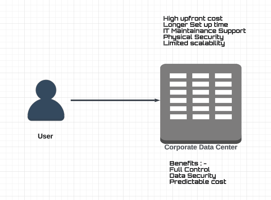
Figure 1 shows a user connecting to an on-prem data center which is self-managed.

A picture containing text, screenshot, diagram, design Description automatically generated

Figure 1: Illustration of a user using on-premises data center.

It is the responsibility of the user or team responsible for managing the infrastructure to ensure that servers are functioning, physically secure, and that software and hardware are regularly maintained and updated. The diagram above highlights certain concerns, including the need for additional personnel for maintenance, high initial costs, and a potentially longer setup process.

On-premises refers to information technology infrastructure hardware and software applications that are hosted on data centers owned/leased by companies. Organizations and businesses have substantial control over the underlying infrastructure.

The key strengths organizations get from on-premises infrastructure are:

  1. Control of hardware and software: Customers exert great control over the hardware and software stacks. Customers can customize their own configurations, upgrades, and system changes.
  2. Fine-grained control in areas of responsibility: Customers have low-level control over governance and regulatory compliance, as well as other areas for which they are solely responsible.
  3. Internet connectivity does not have to be a dependency: An on-premises architecture can be configured so that Internet connectivity does not have to be a requirement for software access. In an on-premises environment, the infrastructure and applications are hosted and managed within the organization’s own physical premises or dedicated data center. The data and services are accessed and operated within the local network, without relying on an external internet connection for their core functionality.
  4. Lower Total Cost of Ownership (TCO): An on-premises architecture can have a lower TCO from a licensing perspective. In an on-premises environment, organizations typically purchase software licenses upfront and own them indefinitely. This means they have the freedom to use the software without ongoing subscription fees or recurring payments. They can negotiate licensing agreements and terms directly with the software vendors, potentially securing better pricing based on their specific needs and usage patterns.
  5. Predictable cost: Organizations have more control over their costs as they make upfront investments in hardware and software. This allows for better cost predictability and the ability to allocate resources according to the organization’s budget and needs.

The on-premises infrastructure does possess a few drawbacks:

  1. Large initial investment: The on-premises infrastructure requires large hardware and software purchases, which represent significant upfront costs. Maintenance, including support and upgrades, represents additional costs.
  2. Longer setup and implementation time: The on-premises infrastructure set-up can take a considerable amount of time for installation, especially for complex systems like a database management system, which typically requires more than just installing a piece of software and letting the users used it.
  3. Responsibility for maintenance: With the on-premises infrastructure, the customer is responsible for maintaining their own server hardware, software, storage, disaster recovery, etc.

What is the Cloud and How Does It Compare to On-Premises Architecture?

The Cloud represents on-demand delivery of IT resources over the Internet. Organizations do not need to manage hardware and software in the Cloud. Instead, customers pay for resources like storage, compute, high availability/disaster recovery, and other services as they use them. Cloud service providers charge customers at well-defined intervals, at a granularity as low as per-second billing for resources. Resources can generally be configured and acquired, configured, and removed easily and quickly (often with a few mouse-clicks), and, hundreds of services are available to customers.

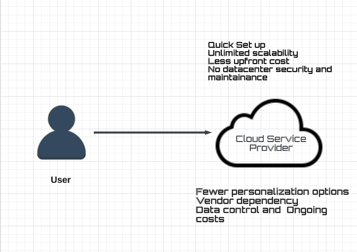
Figure 2 shows a user connecting to a cloud provider.

A diagram of a cloud service provider Description automatically generated with medium confidence

Figure 2: Illustration of a user using cloud services.

The Benefits of Cloud Architecture include

  • Quick deployment: Customers don’t need to provision any hardware, and software can be deployed within minutes. This can drastically reduce time-to-market.
  • Scalability: The biggest advantage of Cloud Computing is that a customer pays only for what they use. In situations where more storage, or greater compute power, is needed, the customer can dynamically and easily scale up their application. In doing so, they pay only for the additional resources used rather than spending money on physical hardware purchases. When the additional resources are no longer needed, the customer can quickly and easily scale down to their normal usage level again.
  • No hardware maintenance: A customer doesn’t need to worry about maintenance of hardware or data center; and physical security is the responsibility of the Cloud provider.
  • Affordable: Cloud providers require no upfront cost. Customers can make regular monthly payments or negotiate a longer-term contract with a Cloud provider to save money and gain more benefits. Customers can start their journey with initial monthly payments and later engage in a longer-term contract when their application is stable, giving them the best of both worlds.
  • Disaster Recovery and Business Continuity: Cloud service providers typically provide reliable disaster recovery and backup solutions. They replicate data across multiple data centers, guaranteeing data resilience and reducing the chances of data loss. This capability allows organizations to swiftly recover from disasters and ensure uninterrupted business operations.
  • Cutting-Edge Technologies: Cloud providers make consistent investments in cutting-edge technologies like artificial intelligence (AI), machine learning (ML), and the Internet of Things (IoT). Through cloud services, organizations can harness the power of these technologies without the requirement of significant infrastructure or specialized expertise in these domains.

The Drawbacks of the Cloud Architecture are:

  • Less customization: Although Cloud providers 100’s of services to choose from and expose many customization options and, customers can apply more fine-grained customizations to their on-premises data centers as compared to Cloud providers. The on-premises model provides greater control over the operating system, software, etc.
  • Long term contracts: Starting with a Cloud provider is often cheaper, but over a long-term period it can be more expensive. This can be due to data transfer costs, moving data in and out of the cloud can be costly, particularly for large volumes of data. After a business has made a commitment to a specific cloud provider, transitioning to an alternative provider can be challenging and may incur considerable expenses and disruptions. As a result, this scenario may result in reduced competition and higher costs over the long run.
  • Connectivity: Using the Cloud requires reliable and sufficient Internet connectivity. Regional, or Internet-wide, Cloud provider outages may adversely affect your productivity.
  • Data Security Concerns: Storing confidential information in the cloud gives rise to apprehensions regarding the security and privacy of data. Organizations must place their trust in the security measures and data handling practices of their chosen cloud service provider. Unauthorized access or breaches in cloud-stored data can lead to significant repercussions.
  • Cost Management: Although cloud architecture provides flexibility and scalability, inadequate management can lead to unforeseen expenses. It is crucial for organizations to closely monitor their usage of cloud resources and optimize their configurations to prevent excessive spending.

Conclusion

While both on-premises and cloud computing offer distinct advantages and disadvantages, I would like to share my perspective on the reasons behind the increasing adoption of cloud computing. The current era is witnessing an unprecedented pace of technological advancement, characterized by the rapid evolution of various technologies. One significant trend in the industry is the increasing adoption of cloud solutions. This shift is primarily motivated by the fact that companies no longer must bear the burden of maintaining specialized expertise. Furthermore, the process of installing software in the cloud is considerably faster compared to the traditional approach of purchasing, installing, and managing costly servers independently.

By embracing cloud solutions, companies can prioritize their core business activities instead of diverting valuable time and resources towards the upkeep of complex infrastructures. Moreover, organizations benefit from the flexibility to easily add or remove resources across different performance classes, enabling swift adjustments to meet changing demands. This eliminates the need for protracted procurement processes that would otherwise consume months of valuable time.

Another advantage lies in the vast array of services offered by cloud service providers. Organizations are not limited to using cloud services solely for storage purposes. Instead, they gain access to a broad range of services spanning numerous domains, expanding their capabilities beyond storage, and empowering them to leverage the full potential of cloud computing.

Overall, the relentless advancement of technology, coupled with the inherent benefits of cloud solutions, has prompted organizations to embrace this paradigm shift. By harnessing the power of the cloud, companies can streamline their operations, focus on core competencies, and avail themselves of a wide array of services to drive innovation and stay competitive in today’s fast-paced digital landscape.


The post On Premises vs Cloud appeared first on Simple Talk.


from Simple Talk https://ift.tt/VoAgae8
via

Thursday, June 1, 2023

SQL Server 2022: Capture SQL Anti-Patterns

 
One of the new Extended Event available in SQL Server 2022 is the query_antipattern. This extended event allows to identify anti-patterns on the SQL queries sent to the server.  An anti-pattern in this case is some code that the SQL Server optimizer can’t do a great job optimizing the code (but cannot correct the issue automatically).
 
This is a very interesting possibility: Including this event in a session allow us to identify potential problems in applications. We can do this in development environments to the the problems earlier in the SDLC (Software Development Life Cycle).  Let’s replicate some examples and check how this works.
 

Requirements

If you want to follow along with the examples, you need to install the sample database WideWorldImporters. You can download it on this link https://github.com/Microsoft/sql-server-samples/releases/tag/wide-world-importers-v1.0
 
After downloading and restoring the database,  you need to create a new index on Sales.Orders using the code below:
USE [WideWorldImporters]
GO

CREATE NONCLUSTERED INDEX [indPurchaseOrder]
  ON [Sales].[Orders] ( [customerpurchaseordernumber] ASC )
GO

Prepare the Extended Events Session

Create the Extended Event Session using the following code. (The Extended Event output will be solely to the ring buffer, which lets you view the data easily in SSMS and is good for quick viewing of extended session output.)
USE master;
GO 

IF EXISTS (SELECT * 
           FROM   sys.dm_xe_sessions 
           WHERE  NAME = 'query_antipattern_xe') 
  BEGIN 
      DROP event session [query_antipattern_xe] ON server; 
  END
GO 

CREATE EVENT SESSION [query_antipattern_xe] ON SERVER  
     ADD EVENT sqlserver.query_antipattern (   
        ACTION(sqlserver.client_app_name,sqlserver.plan_handle, 
               sqlserver.query_hash,sqlserver.query_plan_hash,
               sqlserver.sql_text)
          ) ADD TARGET package0.ring_buffer(SET max_memory=(500)) 
GO
Start the Extended Event Session using the following code:
ALTER EVENT SESSION query_antipattern_xe ON SERVER
STATE = START;
GO
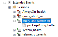
Then verify it is started in management studio:
 
 
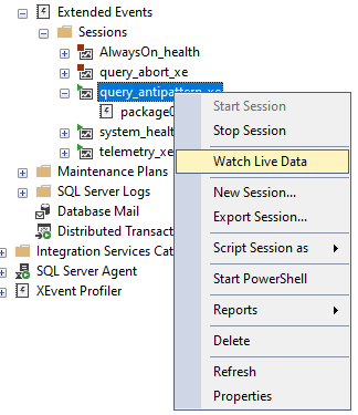
Right-click the session and select the Watch Live Data menu item. This will let you see as new events occur.


Anitpattern #1 – Implicit conversions

One of the biggest silent performance killers in T-SQL code is certain implicit conversions where the comparison cannot be performed in a lossless manner.  For an example, in a new query window, execute the script to cause the first anti-pattern:
USE WideWorldImporters
GO

SELECT *  
FROM    Sales.Orders 
WHERE  CustomerPurchaseOrderNumber=10014;
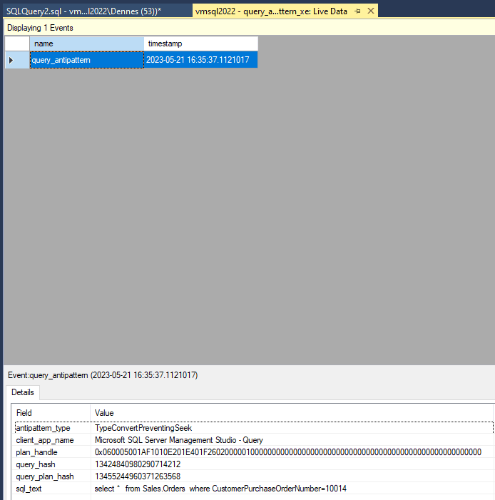
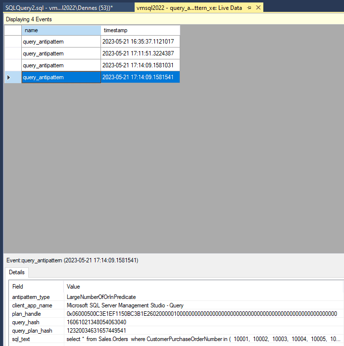
Check the Live Data window to see the anti-pattern capture
 
 
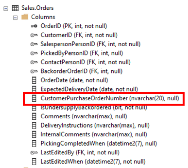
You can see in the antipattern_type row that this is a TypeConvertPreventingSeekevent.  SQL Server is capable of automatically converting data types in a query. The field type is NVARCHAR and the query parameter is INT. Some automatic query conversions prevent the use of index seek, typically where the conversion may be lossless. 
 
 
Because of how conversions work, if you look a the query plan for this query, you will see that the CustomerPurchaseOrderNumber column is converted to an integer for the comparison. Each row has to be converted, so the index cannot be used. Relying on automatic data type conversions in predicates is considered an anti-pattern. If any value in the column was not able to be converted to an INT value, the query would have failed.
 
While it is always a good practice to match your parameter or search criteria to the datatype of your column, this anti-pattern is only captured when it actually prevents the Index Seek. For example, if you changed the predicate to WHERE CustomerPurchaseOrderNumber=CAST('10014' as char(10)); you will still see the implicit conversion, but since the ASCII value can be losslessly changed to a UNICODE value, the index can be used, and no anti-pattern event is raised.
 

Anitpattern #2 – Large IN expressions

To demonstrate this antipattern, I will use the following query that has 150 items in the IN expression of the WHERE clause.

SELECT * 
FROM   Sales.Orders 
WHERE  CustomerPurchaseOrderNumber IN ( 10001,10002,10003,10004,10005,
10006,10007,10008,10009,10010,10011,10012,10013,10014,10015,10016,10017,
10018,10019,10020,10021,10022,10023,10024,10025,10026,10027,10028,10029,
10030,10031,10032,10033,10034,10035,10036,10037,10038,10039,10040,10041,
10042,10043,10044,10045,10046,10047,10048,10049,10050,10051,10052,10053,
10054,10055,10056,10057,10058,10059,10060,10061,10062,10063,10064,10065,
10066,10067,10068,10069,10070,10071,10072,10073,10074,10075,10076,10077,
10078,10079,10080,10081,10082,10083,10084,10085,10086,10087,10088,10089,
10090,10091,10092,10093,10094,10095,10096,10097,10098,10099,10100,10101,
10102,10103,10104,10105,10106,10107,10108,10109,10110,10111,10112,10113,
10114,10115,10116,10117,10118,10119,10120,10121,10122,10123,10124,10125,
10126,10127,10128,10129,10130,10131,10132,10133,10134,10135,10136,10137,
10138,10139,10140,10141,10142,10143,10144,10145,10146,10147,10148,10149,
10150);
Note: this query was created using by taking the following query code:
SELECT * 
FROM   Sales.Orders 
WHERE  CustomerPurchaseOrderNumber IN ( );
And generating the IN expression using 
SELECT STRING_AGG( CustomerPurchaseOrderNumber,',')
FROM ( SELECT DISTINCT TOP 150 CustomerPurchaseOrderNumber
       FROM Sales.Orders) Orders;
Just paste the output into the parenthesis. Next, select and execute the query. Check the Watch Live Data window and you should see some new activity.
 
 
The Anti-Pattern identified is the LargeNumberOfOrInPredicate. The IN predicate in fact is translated as a series of OR logical conditions which cannot be optimized, resulting in this anti-pattern. Part of why this is noted as an anti-pattern is that the TypeConvertPreventingSeekevent occurs as well because we are again comparing NVARCHAR to INT types. 
 
If you change the IN expression to use a character type (either Unicode or ASCII), you will not get the warning because just like with the previous example, if it has no direct negative on the optimization of the query, it will not raise the event. You can generate the IN expression as Unicode values using the following query:
SELECT STRING_AGG( 'N''' + CustomerPurchaseOrderNumber + '''',',')
FROM ( SELECT DISTINCT TOP 150 CustomerPurchaseOrderNumber
       FROM Sales.Orders) Orders;

Identifying Additional Anti-Patterns

When looking at the output from the Extended Event, the anti-pattern is identified on the antipattern_type field. We can get the possible values of the antipattern_type field from the extended events system tables and in this way identify what are the possible anti-patterns this event can track.
 
Execute the query below:
SELECT map_value 
FROM sys.dm_xe_map_values 
WHERE name = N'query_antipattern_type';
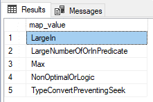
This returns:
 
 
Let’s analyze the result of the query for what the other types of anti-patters might be::
  • TypeConvertPreventingSeek and LargeNumberOfOrInPredicate: These are the two anti-patterns we tested
  • LargeIn: The name explains a lot, but when executing a query with a lot of values in anIN expression, the anti-pattern identified is the LargeNumberOfOrInPredicate. It’s not clear what makes the LargeIn to be identified.
  • Max and NonOptimalOrLogic : There is not enough documentation about these two.

Azure SQL Databases

This extended event is also available in Azure SQL Databases. You can read more about how to capture this event on this link https://www.red-gate.com/simple-talk/blogs/azure-sql-extended-events-and-the-use-of-slash/

Conclusion

This extended event has a considerable potential and we should enable it in SQL Servers 2022. However, the anti-patterns identified are still limited and lacking documentation, we should follow the evolution of this event on future SQL Server cumulative updates.
 
One additional thing to note. this can be a very noisy event, especially if you have these events occuring frequently in your application for one, but simple queries of the system views may also cause events to fire. For example, Aaron Bertrand notes in his T-SQL Tuesday Blog from Septemever 2022 that SELECT * FROM sys.database_principals; will cause an implicit conversion (Query_Antipattern_Type: TypeConvertPreventingSeek) event to occur. Aaron provides some advice on how to set up your events that can help mitigate the noisiness.


The post SQL Server 2022: Capture SQL Anti-Patterns appeared first on Simple Talk.


from Simple Talk https://ift.tt/X4uF8EA
via

Wednesday, May 31, 2023

The Importance of Tact

The concept of tact is simple. Telling people truths, often harsh truths, without making it seem harsh. Hopefully, it is clear that being truthful is one of the more essential things in life. As a person in technology (and certainly as an editor), we often need to be honest when the truth hurts a bit more than average.

For example, consider the security manager dealing with one of their coworkers who just clicked on a phishing link that caused the company to lose an hour of data (or day or week.) Without more information, it seems clear that the coworker should be escorted off the premises. Well, at least after listening to a 20-hour rant that would take this blog post from a general audience rating to something far closer than a full-on mature rating.

With these extreme consequences in mind, the next step is determining who this security lecture will be directed at. A recent hire, a company veteran, the CIO, maybe even the company’s owner. How you handle this situation requires knowledge of the audience and shovelfuls of tact based on who the perpetrator turns out to be. You probably can’t terminate the owner, but if you are not tactful enough in handling that situation, whoever replaces you will probably be quite tactful when helping you carry your personal effects to the car.

Most of the time, the need is more subtle than this. You might be leading a code review, a design meeting, or tech editing a piece of writing. Letting others know their shortcomings and failures in a way that informs them without crushing them is a delicate balance. For example, coaching a 10-year-old football team (no matter what you think of when you hear football) is far different than coaching a professional team. Even though it is essentially the same game, the necessary skills to be a coach are very different.

On the other hand, there is one person in this world you should not be tactful with. If you want to pause to think of all the funny answers, the webpage will wait as long as you need. Unfortunately, this person who needs the least tact is often the one you are most tactful with, trying to make this person feel better about everything they do.

The person you be the least tactful with is yourself.

If telling your company owner that they were the cause of a million dollars worth of data damage because they clicked on a link that was supposed to help out their private life is hard… telling yourself the same thing is almost impossible. Oh, I was distracted. I thought that was an actual link… everything except that you messed up, and it is your fault, and you must do better.

Most of us have lied to ourselves for so long about so many things we don’t even know the truth. Some of us hold ourselves in such high regard we can’t even see our limitations. Reminding yourself that you aren’t able to do something is one of the most brutal truths we need to tell ourselves.

The post The Importance of Tact appeared first on Simple Talk.


from Simple Talk https://ift.tt/md1ibpP
via

Monday, May 29, 2023

T-SQL Gap-Filling Challenge

A student of mine sent me a T-SQL challenge involving gap-filling of missing dates and balances. I found the challenge interesting and common enough and figured that my readers would probably find it interesting to work on as well.

I’ll present the challenge and three possible solutions, as well as the results of a performance test. AS always, I urge you to try and come up with your own solutions before looking at mine.

If you would like to download the code including the solutions, you can find it in a .zip file here.

The Challenge

The challenge involves two tables called Workdays and Balances. The Workdays table holds the dates of all workdays going back a few years. The Balances table holds account IDs, dates of workdays when the account balance changed, and the balance on the current date. There’s a foreign key on the date column in the Balances table referencing the date column in the Workdays table.

Use the following code to create the Workdays and Balances tables:

SET NOCOUNT ON;

USE tempdb;

DROP TABLE IF EXISTS dbo.Balances, dbo.Workdays;
GO

CREATE TABLE dbo.Workdays
(
  dt DATE NOT NULL,
  CONSTRAINT PK_Workdays PRIMARY KEY(dt)
);

CREATE TABLE dbo.Balances
(
  accountid INT NOT NULL,
  dt DATE NOT NULL
    CONSTRAINT FK_Balances_Workdays REFERENCES dbo.Workdays,
  balance NUMERIC(12, 2) NOT NULL,
  CONSTRAINT PK_Balances PRIMARY KEY(accountid, dt)
);

Note that the definition of the primary key constraint on Workdays results in a clustered index with dt as the key. Similarly, the definition of the primary key constraint on Balances results in a clustered index with (accountid, dt) as the key.

To generate the sample data for this challenge, you will need a helper function that returns a sequence of integers in a desired range. You can use the GetNums function for this purpose, which you create using the following code:

CREATE OR ALTER FUNCTION dbo.GetNums
      (@low AS BIGINT = 1, @high AS BIGINT)
  RETURNS TABLE
AS
RETURN
  WITH
    L0 AS ( SELECT 1 AS c 
            FROM (VALUES(1),(1),(1),(1),(1),(1),(1),(1),
                        (1),(1),(1),(1),(1),(1),(1),(1)) AS D(c) ),
    L1 AS ( SELECT 1 AS c FROM L0 AS A CROSS JOIN L0 AS B ),
    L2 AS ( SELECT 1 AS c FROM L1 AS A CROSS JOIN L1 AS B ),
    L3 AS ( SELECT 1 AS c FROM L2 AS A CROSS JOIN L2 AS B ),
    Nums AS ( SELECT ROW_NUMBER() 
                       OVER(ORDER BY (SELECT NULL)) AS rownum
              FROM L3 )
  SELECT TOP(@high - @low + 1)
     rownum AS rn,
     @high + 1 - rownum AS op,
     @low - 1 + rownum AS n
  FROM Nums
  ORDER BY rownum;

Alternatively, if you’re using SQL Server 2022 or Azure SQL Database, you can use the built-in GENERATE_SERIES function instead. In my examples I’ll use the GetNums function.

Use the following code to populate the Workdays table with dates in 2013 through 2022 excluding weekends as sample data:

DECLARE @start AS DATE = '20130101', @end AS DATE = '20221231';

INSERT INTO dbo.Workdays(dt)
  SELECT A.dt
  FROM dbo.GetNums(0, DATEDIFF(day, @start, @end)) AS N
    CROSS APPLY (VALUES(DATEADD(day, N.n, @start))) AS A(dt)
  -- exclude Saturday and Sunday
  WHERE DATEDIFF(day, '19000107', dt) % 7 + 1 NOT IN (1, 7);

Normally, dates of holidays would also be excluded from the table, but for our testing purposes we can keep things simple and just exclude weekends.

As for the Balances table; to check the logical correctness of your solutions, you can use the following code, which populates the table with a small set of sample data:

TRUNCATE TABLE dbo.Balances;

INSERT INTO dbo.Balances(accountid, dt, balance)
  VALUES(1, '20220103', 8000.00),
        (1, '20220322', 10000.00),
        (1, '20220607', 15000.00),
        (1, '20221115', 7000.00),
        (1, '20221230', 4000.00),
        (2, '20220118', 12000.00),
        (2, '20220218', 14000.00),
        (2, '20220318', 16000.00),
        (2, '20220418', 18500.00),
        (2, '20220518', 20400.00),
        (2, '20220620', 19000.00),
        (2, '20220718', 21000.00),
        (2, '20220818', 23200.00),
        (2, '20220919', 25500.00),
        (2, '20221018', 23400.00),
        (2, '20221118', 25900.00),
        (2, '20221219', 28000.00);

The task involves developing a stored procedure called GetBalances that accepts a parameter called @accountid representing an account ID. The stored procedure should return a result set with all existing dates and balances for the input account, but also gap-filled with the dates of the missing workdays between the existing minimum and maximum dates for the account, along with the last known balance up to that point. The result should be ordered by the date.

Once you have written your code, you can use the following code to test your solution for correctness with account ID 1 as input:

EXEC dbo.GetBalances @accountid = 1;

With the small set of sample data you should get an output with the following 260 rows, shown here in abbreviated form:

dt         balance
---------- --------
2022-01-03 8000.00
2022-01-04 8000.00
2022-01-05 8000.00
2022-01-06 8000.00
2022-01-07 8000.00
...
2022-03-21 8000.00
2022-03-22 10000.00
2022-03-23 10000.00
2022-03-24 10000.00
2022-03-25 10000.00
2022-03-28 10000.00
...
2022-06-06 10000.00
2022-06-07 15000.00
2022-06-08 15000.00
2022-06-09 15000.00
2022-06-10 15000.00
2022-06-13 15000.00
...
2022-11-14 15000.00
2022-11-15 7000.00
2022-11-16 7000.00
2022-11-17 7000.00
2022-11-18 7000.00
2022-11-21 7000.00
...
2022-12-29 7000.00
2022-12-30 4000.00

Test your solution with account ID 2 as input:

EXEC dbo.GetBalances @accountid = 2;

You should get an output with the following 240 rows, shown here in abbreviated form:

dt         balance
---------- --------
2022-01-18 12000.00
2022-01-19 12000.00
2022-01-20 12000.00
2022-01-21 12000.00
2022-01-24 12000.00
...
2022-02-17 12000.00
2022-02-18 14000.00
2022-02-21 14000.00
2022-02-22 14000.00
2022-02-23 14000.00
2022-02-24 14000.00
...
2022-03-17 14000.00
2022-03-18 16000.00
2022-03-21 16000.00
2022-03-22 16000.00
2022-03-23 16000.00
2022-03-24 16000.00
...
2022-04-15 16000.00
2022-04-18 18500.00
2022-04-19 18500.00
2022-04-20 18500.00
2022-04-21 18500.00
2022-04-22 18500.00
...
2022-05-17 18500.00
2022-05-18 20400.00
2022-05-19 20400.00
2022-05-20 20400.00
2022-05-23 20400.00
2022-05-24 20400.00
...
2022-06-17 20400.00
2022-06-20 19000.00
2022-06-21 19000.00
2022-06-22 19000.00
2022-06-23 19000.00
2022-06-24 19000.00
...
2022-07-15 19000.00
2022-07-18 21000.00
2022-07-19 21000.00
2022-07-20 21000.00
2022-07-21 21000.00
2022-07-22 21000.00
...
2022-08-17 21000.00
2022-08-18 23200.00
2022-08-19 23200.00
2022-08-22 23200.00
2022-08-23 23200.00
2022-08-24 23200.00
...
2022-09-16 23200.00
2022-09-19 25500.00
2022-09-20 25500.00
2022-09-21 25500.00
2022-09-22 25500.00
2022-09-23 25500.00
...
2022-10-17 25500.00
2022-10-18 23400.00
2022-10-19 23400.00
2022-10-20 23400.00
2022-10-21 23400.00
2022-10-24 23400.00
...
2022-11-17 23400.00
2022-11-18 25900.00
2022-11-21 25900.00
2022-11-22 25900.00
2022-11-23 25900.00
2022-11-24 25900.00
...
2022-12-16 25900.00
2022-12-19 28000.00

Performance Testing Technique

To test the performance of your solutions you will need to populate the Balances table with a larger set of sample data. You can use the following code for this purpose:

DECLARE
  @numaccounts AS INT = 100000,
  @maxnumbalances AS INT = 24,
  @maxbalanceval AS INT = 500000,
  @mindate AS DATE = '20220101',
  @maxdate AS DATE = '20221231';

TRUNCATE TABLE dbo.Balances;

INSERT INTO dbo.Balances WITH (TABLOCK) (accountid, dt, balance)
  SELECT 
      A.accountid, 
      B.dt, 
    CAST(ABS(CHECKSUM(NEWID())) % @maxbalanceval AS NUMERIC(12, 2)) 
                                                          AS balance
  FROM (SELECT n AS accountid, 
               ABS(CHECKSUM(NEWID())) % @maxnumbalances + 1 AS numbalances
        FROM dbo.GetNums(1, @numaccounts)) AS A
    CROSS APPLY (SELECT TOP (A.numbalances) W.dt                   
                 FROM dbo.Workdays AS W
                 WHERE W.dt BETWEEN @mindate AND @maxdate
                 ORDER BY CHECKSUM(NEWID())) AS B;

This code sets parameters for the sample data before filling the table. The performance results that I’ll share in this article were based on sample data created with the following parameter values:

  • Number of accounts: 100,000
  • Number of balances per account: random number between 1 and 24
  • Balance dates: chosen randomly from Workdays within the range 2022-01-01 to 2022-12-31

Using the above parameters, the sample data resulted in about 1,250,000 rows in the Balances table. That’s an average of about 12.5 balances per account before gap filling. After gap filling the average number of balances per account was about 200. That’s the average number of rows returned from the stored procedure.

If you need to handle a similar task in your environment, of course you can feel free to alter the input parameters to reflect your needs.

The requirement from our stored procedure is to have a sub-millisecond runtime as it’s expected to be executed very frequently from many concurrent sessions.

If you’re planning to test your solutions from SSMS, you’d probably want to run them in a loop with many iterations, executing the stored procedure with a random input account ID in each iteration. You can measure the total loop execution time and divide it by the number of iterations to get the average duration per proc execution.

Keep in mind though that looping in T-SQL is quite expensive. To account for this, you can measure the time it takes the loop to run without executing the stored procedure and subtract it from the time it takes it to run including the execution of the stored procedure.

Make sure to check “Discard results after execution” in the SSMS Query Options… dialog to eliminate the time it takes SSMS to print the output rows. Your test will still measure the procedure’s execution time including the time it takes SQL Server to transmit the result rows to the SSMS client, just without printing them. Also, make sure to not turn on Include Actual Execution Plan in SSMS.

Based on all of the above, you can use the following code to test your solution proc with 100,000 iterations, and compute the average duration per proc execution in microseconds:

DECLARE 
  @numaccounts AS INT = 100000, 
  @numiterations AS INT = 100000,
  @i AS INT, 
  @curaccountid AS INT,
  @p1 AS DATETIME2, @p2 AS DATETIME2, @p3 AS DATETIME2,
  @duration AS INT;

-- Run loop without proc execution to measure loop overhead
SET @p1 = SYSDATETIME();
SET @i = 1;
WHILE @i <= @numiterations
BEGIN
  SET @curaccountid = ABS(CHECKSUM(NEWID())) % @numaccounts + 1;
  SET @i += 1;
END;
SET @p2 = SYSDATETIME();

-- Run loop with proc execution
SET @i = 1;
WHILE @i <= @numiterations
BEGIN
  SET @curaccountid = ABS(CHECKSUM(NEWID())) % @numaccounts + 1;
  EXEC dbo.GetBalances @accountid = @curaccountid;
  SET @i += 1;
END;

SET @p3 = SYSDATETIME();
-- Compute average proc execution time, accounting for 
-- loop overhead
SET @duration = (DATEDIFF_BIG(microsecond, @p2, @p3) - 
               DATEDIFF_BIG(microsecond, @p1, @p2)) / @numiterations;

PRINT 
  'Average runtime across '
    + CAST(@numiterations AS VARCHAR(10)) + ' executions: '
    + CAST(@duration AS VARCHAR(10)) + ' microseconds.';

If you also want to measure the number of logical reads, you can run an extended events session with the sql_batch_completed event and a filter based on the target session ID. You can divide the total number of reads by the number of iterations in your test to get the average per proc execution.

You can use the following code to create such an extended event session, after replacing the session ID 56 in this example with the session ID of your session:

CREATE EVENT SESSION [Batch Completed for Session] ON SERVER 
ADD EVENT sqlserver.sql_batch_completed(
    WHERE ([sqlserver].[session_id]=(56)));

One thing that a test from SSMS won’t do is emulate a concurrent workload. To achieve this you can use the ostress tool, which allows you to run a test where you indicate the number of concurrent threads and the number of iterations per thread. As an example, the following code tests the solution proc with 100 threads, each iterating 1,000 times, in quiet mode (suppressing the output):

ostress.exe -SYourServerName -E -dtempdb -Q"DECLARE @numaccounts AS INT = 100000; DECLARE @curaccountid AS INT = ABS(CHECKSUM(NEWID())) % @numaccounts + 1; EXEC dbo.GetBalances @accountid = @curaccountid;" -n100 -r1000 -q

Of course, you’ll need to change “YourServerName” with your server’s name. The ostress tool reports the total execution time of the test. You can divide it by (numthreads x numiterations) to get the average proc execution time.

Next, I’ll present three solutions that I came up with, and report their average runtimes based on both the SSMS and the ostress testing techniques, as well their average number of logical reads.

Solution 1, using TOP

Following is my first solution, which relies primarily on the TOP filter:

CREATE OR ALTER PROC dbo.GetBalances
  @accountid AS INT
AS

SET NOCOUNT ON;

SELECT W.dt,
   (SELECT TOP (1) B.balance
    FROM dbo.Balances AS B
    WHERE B.accountid = @accountid
      AND B.dt <= W.dt
    ORDER BY B.dt DESC) AS balance
FROM dbo.Workdays AS W
WHERE W.dt BETWEEN (SELECT MIN(dt) 
                    FROM dbo.Balances 
                    WHERE accountid = @accountid)
               AND (SELECT MAX(dt) 
                    FROM dbo.Balances 
                    WHERE accountid = @accountid)
ORDER BY W.dt;

This is probably the most obvious solution that most people will come up with intuitively.

The code queries the Workdays table (aliased as W), filtering the dates that exist between the minimum and maximum balance dates for the account. In the SELECT list the code returns the current workday date (W.dt), as well as the result of a TOP (1) subquery against Balances (aliased as B) to obtain the last known balance. That’s the most recent balance associated with a balance date (B.dt) that is less than or equal to the current workday date (W.dt). The code finally orders the result by W.dt.

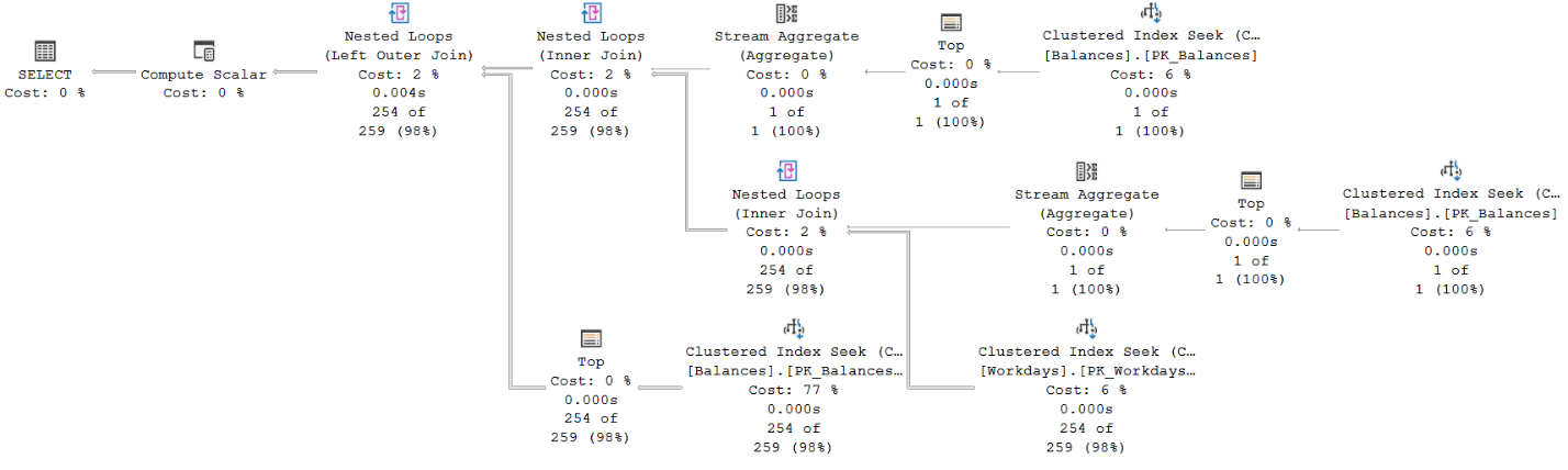
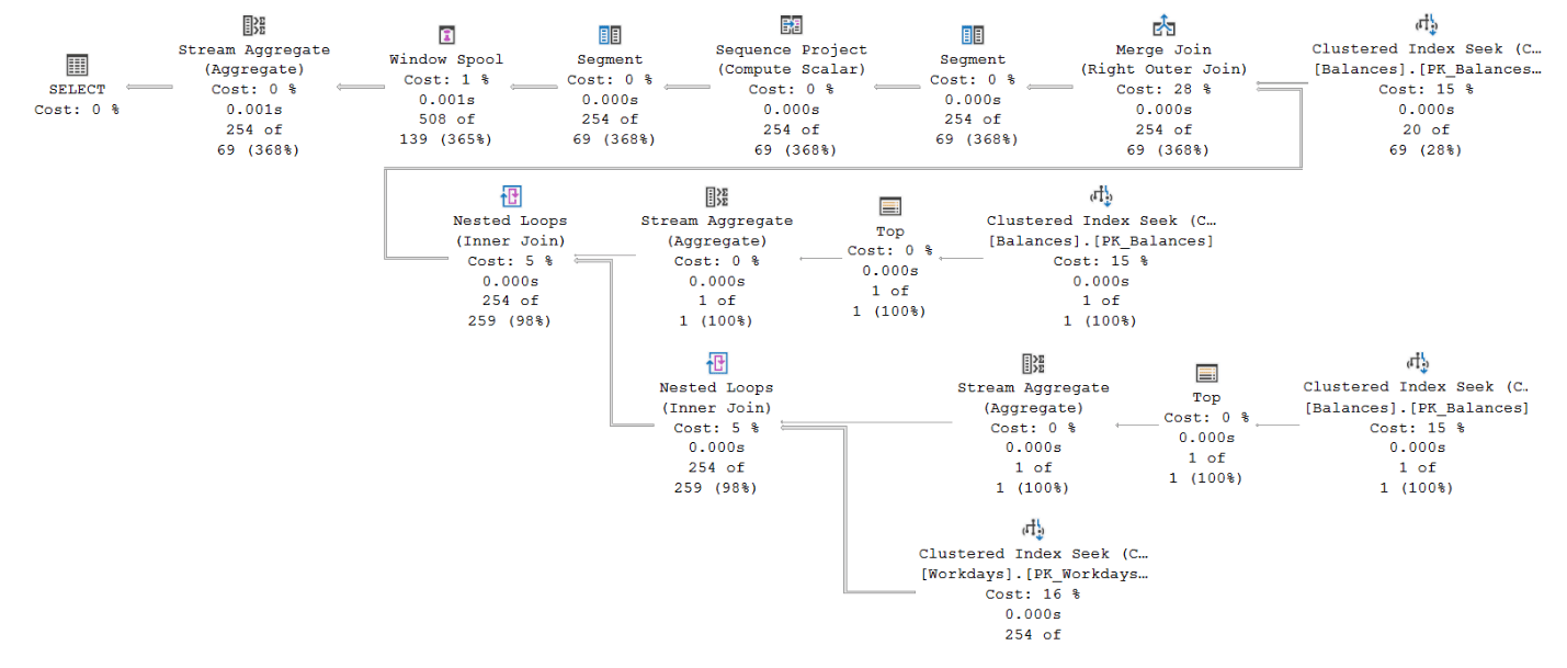
The plan for Solution 1 is shown in Figure 1.

Figure 1: Plan for Solution 1

The top two seeks against the Balances clustered index obtain the minimum and maximum balance dates for the account. Each involves as many logical reads as the depth of the index (3 levels in our case). These two seeks represents a small portion of the cost of the plan (12%).

The bottom right seek against the Workdays clustered index obtains the dates of the workdays between those minimum and maximum. This seek involves just a couple of logical reads since each leaf page holds hundreds of dates, and recall that in our scenario, each account has an average of about 200 qualifying workdays. This seek also represents a small portion of the cost of the plan (6%).

The bulk of the cost of this plan is associated with the bottom left seek against the Balances clustered index (77%). This seek represents the TOP subquery obtaining the last known balance, and is executed per qualifying workday. With an average of 200 qualifying workdays and 3 levels in the index, this seek performs about 600 logical reads across all executions.

Notice that there’s no explicit sorting in the plan since the query ordering request is satisfied by retrieving the data based on index order.

Here are the performance numbers that I got for this solution in average per proc execution:

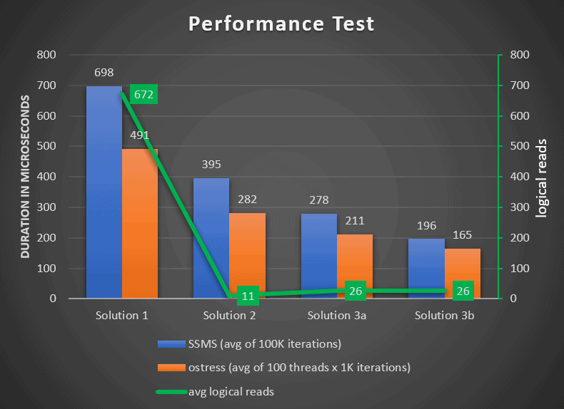
Duration with SSMS test: 698 microseconds

Duration with ostress test: 491 microseconds

Logical reads: 672

Solution 2, using IGNORE NULLS

SQL Server 2022 introduces a number of T-SQL features to support queries involving time-series data. Once specific feature that is relevant to our challenge is the standard NULL treatment clause for offset-window functions (FIRST_VALUE, LAST_VALUE, LAG and LEAD). This feature allows you to specify the IGNORE NULLS clause if you want the function to continue looking for a non-NULL value when the value in the requested position is missing (is NULL). You can find more details about the NULL treatment clause here.

Following is my second solution, which uses the NULL treatment clause:

CREATE OR ALTER PROC dbo.GetBalances
  @accountid AS INT
AS
SET NOCOUNT ON;
SELECT W.dt, 
       LAST_VALUE(B.balance) IGNORE NULLS 
           OVER(ORDER BY W.dt ROWS UNBOUNDED PRECEDING) AS balance
FROM dbo.Workdays AS W
  LEFT OUTER JOIN dbo.Balances AS B
    ON B.accountid = @accountid
    AND W.dt = B.dt
WHERE W.dt BETWEEN (SELECT MIN(dt) 
                    FROM dbo.Balances 
                    WHERE accountid = @accountid)
               AND (SELECT MAX(dt) 
                    FROM dbo.Balances 
                    WHERE accountid = @accountid)
ORDER BY W.dt;
GO

The code performs a left outer join between Workdays and Balances. It matches workday dates that appear between the minimum and maximum balance dates for the account (obtained with subqueries like in Solution 1) with the balance dates for the account. When a match is found, the outer join returns the respective balance on that workday date. When a match isn’t found, the outer join produces a NULL value as the balance.

The SELECT list then computes the last known balance using the LAST_VALUE function with the IGNORE NULLS clause.

Like in Solution 1, this solution’s code returns the data ordered by W.dt.

The plan for Solution 2 is shown in Figure 2.

Figure 2: Plan for Solution 2

The topmost seek in the plan against the Balances clustered index retrieves the balances for the account. The cost here is 3 logical reads.

The two seeks in the middle of the plan against the Balances clustered index retrieve the minimum and maximum balance dates for the account. Each costs 3 logical reads.

The bottom seek against the Workdays clustered index retrieves the workday dates in the desired range. It costs a couple of logical reads.

The Merge Join (Right Outer Join) operator merges the workday dates with the respective balance dates based on index order, preserving the workday dates.

Finally, the operators to the left of the Merge Join operator compute the LAST_VALUE function’s result, applying the logic relevant to the IGNORE NULLS option.

Like with Solution 1’s plan, this solution’s plan has no explicit sorting since the query ordering request is satisfied by retrieving the data based on index order.

Here are the performance numbers that I got for this solution in average per proc execution:

Duration with SSMS test: 395 microseconds

Duration with ostress test: 282 microseconds

Logical reads: 11

As you can see, that’s a significant improvement in runtime and a dramatic improvement in I/O footprint compared to Solution 1.

Solutions 3a and 3b, Matching Balance Date Ranges with Workdays

The characteristics of our data are that there are very few balances per account (an average of 12.5), and many more applicable workdays (an average of about 200). With this in mind, a solution that starts with Balances and then looks for matches in Workdays could potentially be quite optimal, as long as it also gets optimized this way. Here’s solution 3a implements this approach:

CREATE OR ALTER PROC dbo.GetBalances
  @accountid AS INT
AS
SET NOCOUNT ON;
WITH C AS
(
  SELECT B.dt, B.balance,
         LEAD(B.dt) OVER(ORDER BY B.dt) AS nextdt
  FROM dbo.Balances AS B
  WHERE accountid = @accountid
)
SELECT ISNULL(W.dt, C.dt) AS dt, C.balance
FROM C
  LEFT OUTER JOIN dbo.Workdays AS W
    ON W.dt >= C.dt AND W.dt < C.nextdt
ORDER BY dt;
GO

The query in the CTE called C uses the LEAD function to create current-next balance date ranges.

The outer query then uses a left outer join between C and Workdays (aliased as W), matching each balance date range with all workday dates that fall into that date range (W.dt >= C.dt AND W.dt < C.nextdt).

The SELECT list returns the first non-NULL value among W.dt and C.dt as the result dt column, and C.balance as the effective balance on that date.

The outer query returns the result ordered by the result column dt.

The plan for Solution 3a in Figure 3.

Figure 3: Plan for Solution 3a

The top seek against the clustered index on balances retrieves the balances for the account. This seek costs 3 logical reads. The remaining operators to the left of the seek and before the Nested Loops operator compute the LEAD function’s result, relying on index order. Then, a seek is applied against the clustered index on Workdays per balance date range. In average, you get 12.5 seeks, each costing a couple of reads.

The one tricky thing in this plan is that there’s a Sort operator used to handles the query’s presentation ordering request. The explicit sorting is needed since the ordering expression is a result of a computation with the ISNULL function. That’s similar to breaking SARGability when applying manipulation on the filtered column. Since we’re talking about a couple hundred rows that need to be sorted in average, the sort is not a disaster, but it does require a memory grant request, and it does cost a bit.

Here are the performance numbers that I got for this solution in average per proc execution:

Duration with SSMS test: 278 microseconds

Duration with ostress test: 211 microseconds

Logical reads: 26

Even though the number of logical reads is a bit higher than for Solution 2, the runtime is an improvement.

If we could just get rid of the explicit sorting though! There is a neat trick to achieve this. Remember, the sorting is required due to the fact that the ordering expression is the result of a computation with the ISNULL function. You can still get the correct ordering without manipulation by ordering by the composite column list C.dt, W.dt.

Here’s solution 3b implements this approach:

CREATE OR ALTER PROC dbo.GetBalances
  @accountid AS INT
AS
SET NOCOUNT ON;
WITH C AS
(
  SELECT B.dt, B.balance,
         LEAD(B.dt) OVER(ORDER BY B.dt) AS nextdt
  FROM dbo.Balances AS B
  WHERE accountid = @accountid
)
SELECT ISNULL(W.dt, C.dt) AS dt, C.balance
FROM C
  LEFT OUTER JOIN dbo.Workdays AS W
    ON W.dt >= C.dt AND W.dt < C.nextdt
ORDER BY C.dt, W.dt;
GO

The plan for Solution 3b in Figure 4.

Figure 4: Plan for Solution 3b

Voila! The plan is similar to that of Solution 3a, but the sort is gone.

Here are the performance numbers I got for this solution:

Duration with SSMS test: 196 microseconds

Duration with ostress test: 165 microseconds

Logical reads: 26

That’s a pretty nice improvement compared to the performance numbers that we started with for Solution 1.

Performance Summary

Figure 5 shows the performance test results. It has the average runtimes using both the SSMS test and the ostress test summarized as bar charts corresponding to the left Y axis, and the line chart representing the average logical reads corresponding to the right Y axis.

Figure 5: Performance Test Summary

Conclusion

In this article I covered a gap-filling challenge that involved gap-filling balances with missing workday dates, and for each reporting the last known balance. I showed three different solutions including one that uses a new time-series related feature called the NULL treatment clause.

As you can imagine, indexing and reuse of cached query plans were paramount here, and both were handled optimally. Using a good representative sample data that adequately represents the production environment, and an adequate testing technique are also important.

The performance expectations were for a sub-millisecond runtime in a concurrent workload, and this requirement was achieved. In fact, all solutions satisfied this requirement, with the last taking less than 200 microseconds to run.


The post T-SQL Gap-Filling Challenge appeared first on Simple Talk.


from Simple Talk https://ift.tt/1aNvUI4
via
Saturday, May 27, 2023

Unmasking SQL Server Dynamic Data Masking, Part 1, Intro

This is the beginning of a series on SQL Server Dynamic Data Masking. Dynamic Data Masking is a concept familiar with all developers and users of sensitive data. It is implemented in SQL Server with simplicity and elegance, requiring minimal changes to front end applications, including reporting, and almost no changes to queries. The series includes:

  1. An in-depth introduction and use cases
  2. Setup, examples, testing recommendations, coding alternatives to Dynamic Data Masking
  3. Side-channel attacks
  4. Attack mitigations and general architectural-considerations

The dynamic data masking feature was introduced in SQL Server 2016. Data masking addresses gaps in exposing data to end users when direct access is allowed via reporting tools, data analysis, machine learning, or any query tool. Masking is used to protect sensitive or proprietary data from users not authorized to view that data by obfuscating the actual data with a mask as it is returned to the user. Stated simply, actual data is not returned to the user but rather replaced with a traditional style mask hiding all or part of the configured column.

For instance, instead of seeing your coworker’s actual salary, something like 000.00 would be returned. Instead of seeing the proprietary name for a product, the mask of xxx would be returned. The mask can be all zeroes, in the case of a number, all x’s for characters, a pre-designated mask, or a completely custom mask.

When using front end applications with built in masking capabilities or custom code, this need has long been addressed. SQL Server dynamic masking instead addresses the masking need directly in the data engine. Implementing masking in the engine ensures data is protected regardless of the access method, reducing the work necessary to mask data in multiple user interfaces and reducing the chance of exposing unmasked data. The engine only presents data based on the security model, including masked or unmasked data.

In this introduction blog, I want to do two things. First, introduce masking as a general topic. Then as an appendix to this post, include the code to setup the rest of the series.

Competing Solutions

Other products exist that actually modify the data in the database, typically referred to as static data masking. This can be useful for moving production data to non-production environments. Since the data is actually modified, even users with escalated privileges in these environments can’t override security and view the proprietary data. Data masked dynamically makes no actual changes to your data

The prime use case for physically masking the data is providing a cleansed copy of production data to non-production environments. This contrasts with dynamic data masking, with a use case of hiding sensitive data in production environments. They address very different use cases and some architectures may require both types of products.

Developers and other users with elevated privileges can easily bypass dynamic data masking in non-production environments. Since non-production environments aren’t typically monitored as closely as production environments, physically masking the data in these environments is a good option.

Static masking can be especially important if government regulations are involved or any other situation where the chance of a data breach has to be reduced to the absolute minimum, which as a data professional, should be practically always. With static data masking, the original data is secure since it has been modified. But because the data is modified, some functionality is lost. Connections to external systems, some front-end application functionality, and some testing scenarios are difficult if not impossible.

Considering that the primary function of a database engine is maintaining data and ensuring the integrity of that data, there aren’t many scenarios when static data masking is appropriate for production. Dynamic data masking requires careful planning and a dedicated plan to be sure it works. Modifying the data requires more planning and time.

Alternate Solutions

Dynamic masking is presented as a possible solution when users are allowed to directly query data. There are caveats to this recommendation, including security concerns presented in later sections. Direct ad-hoc access to data isn’t typically something you should allow your users to do against production transactional systems, so that wouldn’t be a recommended use case. That leaves us with warehouses and reporting systems as the obvious candidates.

Using production data is often necessary to thoroughly test systems, especially system integrations. It can take an unfeasible amount of effort to setup data in all necessary interconnected systems and it is likely to still leave gaps in testing scenarios. It is possible to lock down the target data by means other than data masking. Separate schemas, alternate column names, encrypted columns, lookup tables with alternate keys, or simply excluding the target data are all possibilities depending on the business requirements. The primary strength of dynamic data masking is the low effort to implement. Testing and automatic upgrades done by Microsoft is another big strength. It is much harder to justify a custom solution when something is built into the product, patched, and enhanced by the vendor. Dynamic data masking can also be combined with restricting access via views and stored procedures to make it a more secure solution.

SQL Server’s Always Encrypted is another useful solution that meets a different need. The data is encrypted before it reaches the database engine. Client applications have the encryption key, usually in a key store, and send and receive encrypted data to the engine. It is up to the client application to mask data if that functionality is needed. One benefit of Always Encrypted is that data is encrypted before it hits the data engine. This means that even privileged users, such as administrators, can’t see an unencrypted version of the data. Only authorized application users see the data.

Dynamic Data Masking Security

When configured for a column, dynamic data masking is applied for all users unless they have specific authorization to view the unmasked data. Users need to be granted the UNMASK, ALTER ANY MASK, or CONTROL permission on the database to view unmasked data. Starting with SQL Server 2022, the UNMASK permission is more granular and allows unmasking down to a column level.

Supersets of these permission sets are included in the dbo database role and the sysadmin server role. If users only have SELECT permissions and they don’t have super user permissions, the data will be masked. When implementing a new security layer it is always important to verify that security is working as expected. In general, SQL Server security is additive, so if a user is accidentally put into a group or role with permission to unmask data, they will have those permissions.

Dynamic Data Masking Use Cases

In this section I want to cover some of the primary use cases for the Dynamic Data Masking feature. While it isn’t perfect (as I will cover in a later blog about how it can be defeated if you aren’t careful), it has some very exciting uses.

Simply Hiding Sensitive Data from Users

The primary purpose of dynamic data masking is to obfuscate proprietary data from unauthorized users. The data isn’t changed, rather it is simply presented to users in a modified format or as a static value, such as 0 for integers. You can choose your own format if desired, so you might choose to include the first characters of a name or number, part of an email address including the @ sign so the data in the column is clear, or almost any user defined format.

It can also be used to hide data for authorized users in non-secure or public environments. Dynamic masking does this at the database engine level, thus making raw data access more secure. So, if data scientists, report users, testers, business analysts, product owners or other users are able to access data directly, it can still be protected. Dynamic queries, reports, data extracts are all protected. Users with unmasking privileges to the table or column see unmodified data.

Note that as noted, there are some security concerns with using Dynamic Data Masking in ad-hoc scenarios.


No Syntax Restrictions

The dynamic portion of dynamic data masking is what makes it powerful. Columns configured with dynamic masking functions exactly like other columns, with the exception that the output differs depending on who accesses the data.

The masked columns can be used to JOIN and for GROUP clauses (the actual value is used, not the masked value you see). It can also be used for WHERE clauses without using the masked values. It can be used in aggregations, functions like substring, in comparison operators, and in joins.

If a column with sensitive data is used as the primary key for a table, and that column is masked, it can still be used as the lookup column in your INNER JOIN while keeping it secure. Histograms based on the salaries of employees while keeping the salaries confidential are possible. Data can be limited to a geographic region without allowing users to see the specific geographic data. All the data can be used for comparison operations, aggregations, joins, any operation normally used by data, while still keeping it reasonably confidential (Later in this series I will show examples of what I mean by “reasonably”.)

This is generally why the feature is mostly for building user interfaces, and not to secure data from nosy ad-hoc users,

Summary

SQL Server Dynamic Data Masking was created to make it easier to obfuscate sensitive data. The relative ease of implementation makes it a nice additional layer when presenting SQL Server data. Future sections include detailed setup examples, caveats for use and security considerations.


——————

Appendix, Preparing the test database:

The database I will be using in subsequent blogs is the sample database WideWorldImporters, available in github, using the latest version available. In this section I will provide instructions for setting up and initializing the database for the following blog entries.

Dynamic data masking was added to multiple tables and columns. The columns chosen were determined purely for demonstration purposes and were not evaluated for business utility.

  1. Restore a copy of WideWorldImporters
    1. For an on-Prem installation, use WideWorldImporters-STANDARD.bak
    2. For an Azure database installation, use WideWorldImporters-STANDARD.bacpac
      1. For verification in Azure, the lowest standard tier was used
      2. The FULL version can be used but requires a higher service tier due to the inclusion of memory optimized tables. If you try to import the FULL version to a low tier model in Azure, you will get the following error:

Warning SQL0: A project which specifies SQL Server 2016 as the target platform may experience compatibility issues with Microsoft Azure SQL Database v12.

Error SQL72014: Framework Microsoft SqlClient Data Provider: Msg 40536, Level 16, State 2, Line 1 ‘MEMORY_OPTIMIZED tables’ is not supported in this service tier of the database.

  1. Add users for testing scripts.
    1. MaskedReader for viewing data in a masked state
    2. UnmaskedReader for viewing data in an unmasked state
USE WideWorldImporters;
GO
 
/*
* Create datbase user without a login
* Add to db_datareader for basic access
* Add to [External Sales] for additional access via RLS
*/
CREATE USER MaskedReader WITHOUT LOGIN;
GO
 
ALTER ROLE db_datareader
ADD MEMBER MaskedReader;
GO
 
ALTER ROLE [External Sales]
ADD MEMBER MaskedReader;
GO
 
 
/*
* Create datAbase user without a login
* Add to db_owner for basic access
* Add to [External Sales] for additional access via RLS
*/
CREATE USER UnmaskedReader WITHOUT LOGIN;
GO
 
ALTER ROLE db_owner
ADD MEMBER UnmaskedReader;
GO
 
ALTER ROLE [External Sales]
ADD MEMBER UnmaskedReader;
  1. Mask columns
    1. As installed, WideWorldImporters has 5 masked columns in the Purchasing.Suppliers table and 5 in the corresponding temporal table, Purchasing.Suppliers_Archive.
    2. The following script adds masking to
      1. Application.Countries
      2. Additional columns to Purchasing.Suppliers
      3. Purchasing.SupplierTransactions
      4. Sales.Customers
      5. Sales.Orders
    3. Note that corresponding columns in temporal tables are automatically masked when the parent table is masked.


USE WideWorldImporters;
GO
 
ALTER TABLE Application.Countries
ALTER COLUMN IsoAlpha3Code
ADD MASKED WITH (FUNCTION = 'default()');
GO
 
ALTER TABLE Purchasing.Suppliers
ALTER COLUMN DeliveryLocation
ADD MASKED WITH (FUNCTION = 'default()');
GO
 
ALTER TABLE Purchasing.Suppliers
ALTER COLUMN InternalComments
ADD MASKED WITH (FUNCTION = 'default()');
GO
 
ALTER TABLE Purchasing.Suppliers
ALTER COLUMN PhoneNumber
ADD MASKED WITH (FUNCTION = 'default()');
GO
 
ALTER TABLE Purchasing.Suppliers
ALTER COLUMN SupplierName
ADD MASKED WITH (FUNCTION = 'default()');
GO
 
ALTER TABLE Purchasing.SupplierTransactions
ALTER COLUMN AmountExcludingTax
ADD MASKED WITH (FUNCTION = 'default()');
GO
 
ALTER TABLE Purchasing.SupplierTransactions
ALTER COLUMN LastEditedWhen
ADD MASKED WITH (FUNCTION = 'default()');
GO
 
ALTER TABLE Purchasing.SupplierTransactions
ALTER COLUMN OutstandingBalance
ADD MASKED WITH (FUNCTION = 'default()');
GO
 
ALTER TABLE Purchasing.SupplierTransactions
ALTER COLUMN SupplierInvoiceNumber
ADD MASKED WITH (FUNCTION = 'default()');
GO
 
ALTER TABLE Purchasing.SupplierTransactions
ALTER COLUMN TaxAmount
ADD MASKED WITH (FUNCTION = 'default()');
GO
 
ALTER TABLE Purchasing.SupplierTransactions
ALTER COLUMN TransactionAmount
ADD MASKED WITH (FUNCTION = 'default()');
GO
 
ALTER TABLE Purchasing.SupplierTransactions
ALTER COLUMN TransactionDate
ADD MASKED WITH (FUNCTION = 'default()');
GO
 
ALTER TABLE Sales.Customers
ALTER COLUMN CreditLimit
ADD MASKED WITH (FUNCTION = 'default()');
GO
 
ALTER TABLE Sales.Customers
ALTER COLUMN CustomerName
ADD MASKED WITH (FUNCTION = 'default()');
GO
 
ALTER TABLE Sales.Customers
ALTER COLUMN DeliveryAddressLine1
ADD MASKED WITH (FUNCTION = 'default()');
GO
 
ALTER TABLE Sales.Customers
ALTER COLUMN DeliveryAddressLine2
ADD MASKED WITH (FUNCTION = 'default()');
GO
 
ALTER TABLE Sales.Customers
ALTER COLUMN DeliveryPostalCode
ADD MASKED WITH (FUNCTION = 'default()');
GO
 
ALTER TABLE Sales.Orders
ALTER COLUMN OrderDate
ADD MASKED WITH (FUNCTION = 'default()');

Setup Notes

https://github.com/Microsoft/sql-server-samples/releases/tag/wide-world-importers-v1.0

WideWorldImporters-STANDARD.bacpac

WideWorldImporters-STANDARD.bak


References

https://learn.microsoft.com/en-us/sql/relational-databases/security/dynamic-data-masking?view=sql-server-ver16

http://wiki.gis.com/wiki/index.php/Decimal_degrees

https://learn.microsoft.com/en-us/sql/t-sql/statements/execute-as-transact-sql?view=sql-server-ver16

https://learn.microsoft.com/en-us/sql/t-sql/queries/with-common-table-expression-transact-sql?view=sql-server-ver16

https://learn.microsoft.com/en-us/sql/relational-databases/security/row-level-security?view=sql-server-ver16

https://learn.microsoft.com/en-us/sql/relational-databases/security/encryption/always-encrypted-tutorial-getting-started?view=sql-server-ver16&tabs=ssms

https://learn.microsoft.com/en-us/sql/relational-databases/security/encryption/always-encrypted-database-engine?view=sql-server-ver16

The post Unmasking SQL Server Dynamic Data Masking, Part 1, Intro appeared first on Simple Talk.


from Simple Talk https://ift.tt/3SwpDvI
via