Thursday, September 7, 2023

Microsoft Fabric: Lakehouse and Data Factory in Power BI environment

Microsoft is merging Data Factory and Power BI Dataflows in one single ETL solution. It’s not a simple merging, but still these ETL tools are easier to use then ever.

In this article, I will demonstrate how to create a lakehouse and ingest data using a step-by-step walkthrough that you can follow along with. You will see that it is not very difficult and what features are available.

If you need a refresher on what Microsoft Fabric is, you can read the first article I wrote here overview of Microsoft Fabric and this other one to enable a free preview so you can try it out without spending money.

Creating the Lakehouse

Let’s create a new lakehouse, step by step.

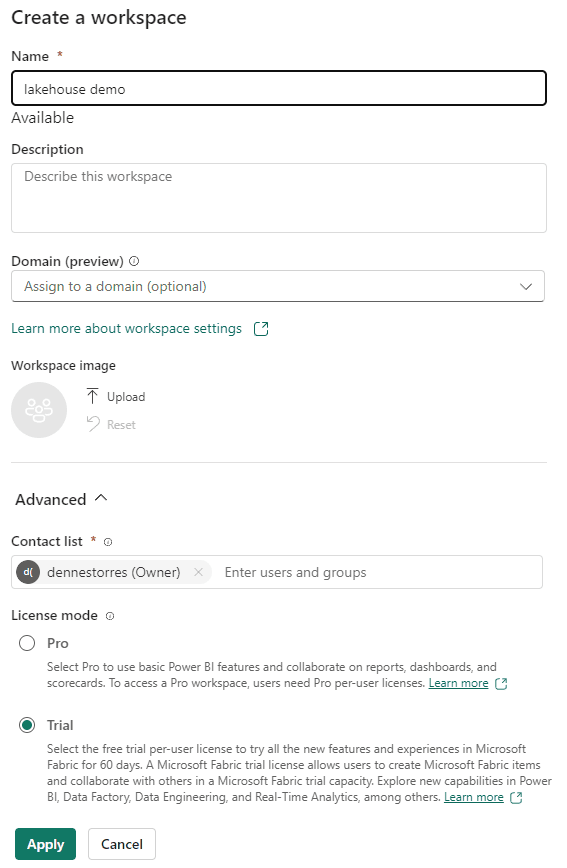
  • Create a new workspace, let’s call it lakehouse demo. Use the trial resources explained here
Interface gráfica do usuário, Texto, Aplicativo, Email Descrição gerada automaticamente 

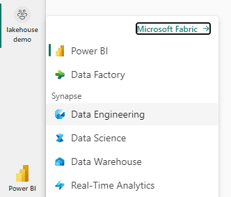
  • Select the Data Engineering Experience
Interface gráfica do usuário, Aplicativo Descrição gerada automaticamente

Tela de computador com texto preto sobre fundo branco Descrição gerada automaticamente com confiança média

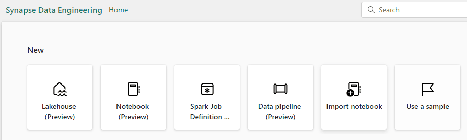
Synapse is present everywhere. The title of the window appears as Synapse Data Engineering

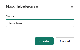
  • Click the Lakehouse button and give it a name, demolake (or whatever you want to, but in the article it will be named demolake)

Interface gráfica do usuário, Texto, Aplicativo, chat ou mensagem de texto Descrição gerada automaticamente

Ingesting Files into the Lakehouse

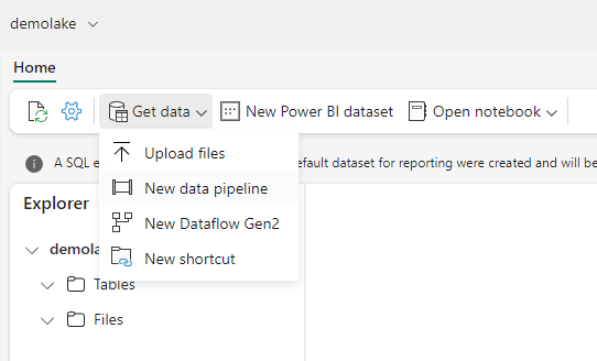
After creating the lakehouse, it’s time to create a data factory pipeline to ingest the data.

  • Click the menu Get Data -> New Data Pipeline

Interface gráfica do usuário, Aplicativo Descrição gerada automaticamente

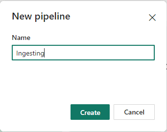
  • Give a name to the pipeline as Ingesting
Interface gráfica do usuário, Texto, Aplicativo, chat ou mensagem de texto Descrição gerada automaticamente

The wizard for data ingestion is one of the new features. It makes the work much easier than in previous iterations of these tools. The next image shows the first window of the wizard.
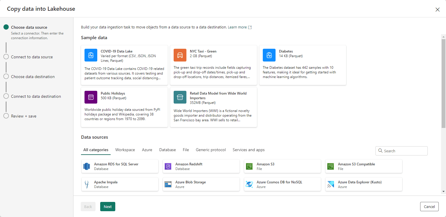
Interface gráfica do usuário, Texto, Aplicativo, Email Descrição gerada automaticamente

We will load information from a sample azure blob storage provided by Microsoft and with anonymous access.

  • Select Azure Blob Storage as the source and click the Next button.
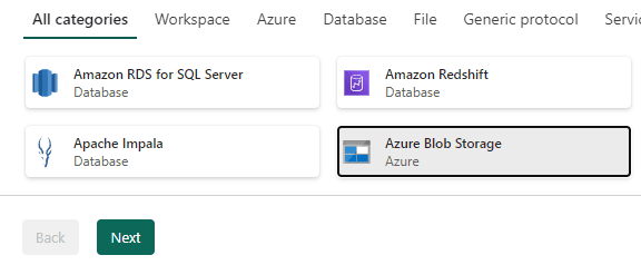
Interface gráfica do usuário Descrição gerada automaticamente

On the following screen, you can choose between an existing connection or a new one. The Power BI environment saves connections to be reused by different objects and this includes Microsoft Fabric objects. You can read more about Power BI and Fabric connection management
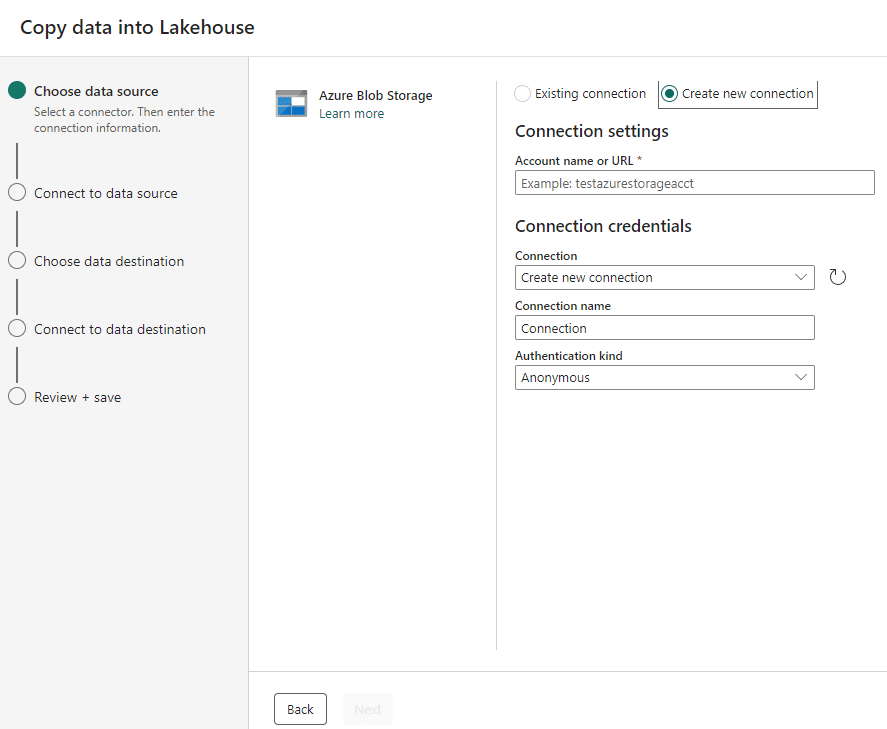
Interface gráfica do usuário, Aplicativo Descrição gerada automaticamente

  • On the Account Name or URL textbox, type the following address: https://ift.tt/oVRdsyO
  • On the Connection Name textbox, type wwisample
  • Click the Next button.

Here we can find how easy a wizard can be: After noticing we don’t have anonymous access direct to the container, the wizard gives us another window to type the precise path we would like to access and get the data from:
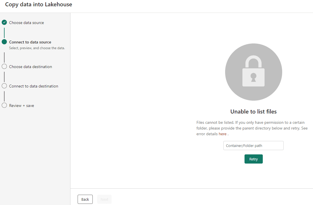
Interface gráfica do usuário, Aplicativo, Teams Descrição gerada automaticamente

  • On the textbox in the middle of the wizard, type the following path: /sampledata/WideWorldImportersDW/parquet
  • Click the Retry button

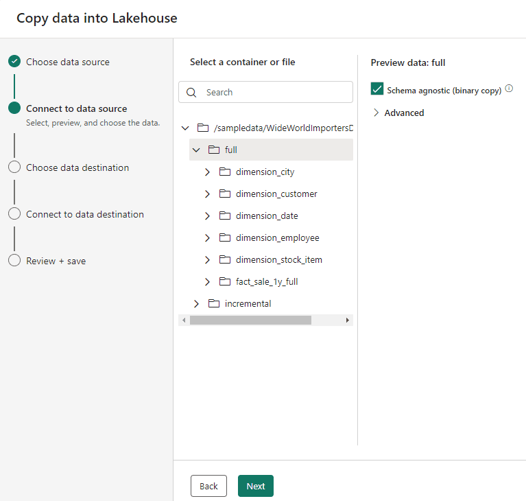
After the retry, we will be able to see the list of folders available for us and the options about the format for ingestion.

  • Select the folder full
  • Mark the checkbox Schema agnostic (binary copy)
Interface gráfica do usuário, Aplicativo Descrição gerada automaticamente

The binary copy option, like the one existing in Data Factory’s Copy Activity, allow us to copy not only multiple files but multiple folders to the Files area of the lakehouse.

The same couldn’t be done to the Tables area of the lakehouse, we would need to import the tables one by one with the correct schema.

  • Click the Next button.
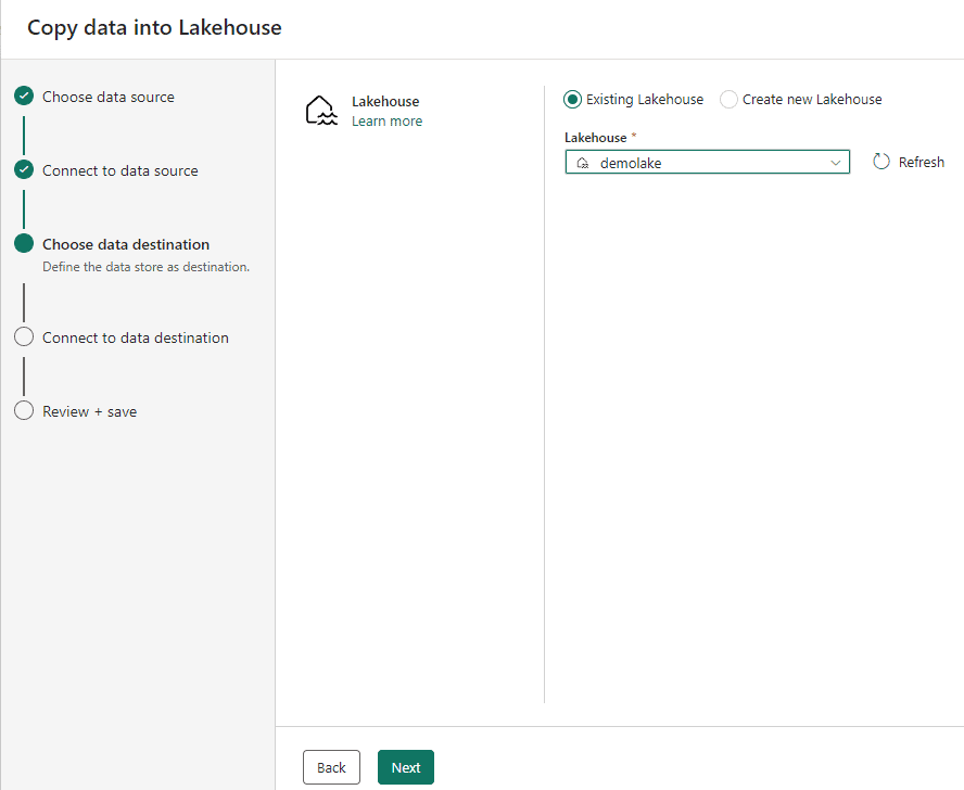
  • Choose the option Existing Lakehouse

Interface gráfica do usuário, Texto, Aplicativo Descrição gerada automaticamente

Choosing the lakehouse is the first option on the destination choice.

  • Click the Next button

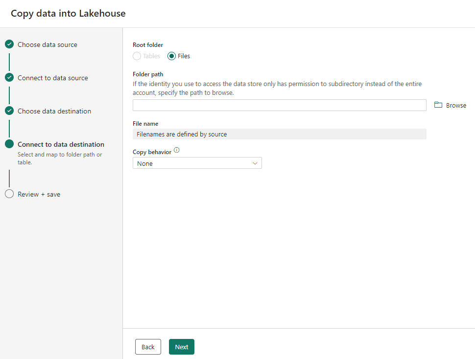
We need to select the destination of the files being copied. The Tables destination is disabled because we selected the binary copy.

The Browse button allow you to organize the files you are copying according to your folder structure. In our example, we don’t have a folder structure yet, so we don’t need to click the Browse button.
Interface gráfica do usuário, Texto, Aplicativo, Email Descrição gerada automaticamente

  • Click the Next button

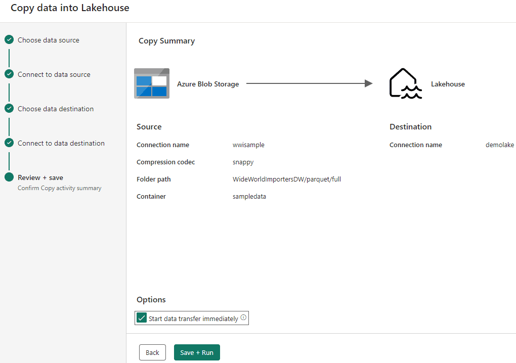
At this point, all the configuration needed for the ingestion is done. We only need to conclude the Wizard and ask for the execution.

  • Mark the checkbox Start data transfer immediately.
  • Click the Save + Run button.

Interface gráfica do usuário, Aplicativo Descrição gerada automaticamente

The pipeline will be executed, and you may notice it’s a simple Copy Activity, which is usual for a Data Factory Pipeline. As explained, the pipelines and dataflows in Microsoft Fabric are a merge between Power BI and Data Factory features.


Interface gráfica do usuário, Texto, Aplicativo Descrição gerada automaticamente

Interface gráfica do usuário, Texto, Aplicativo Descrição gerada automaticamente

  • Click the demolake button on the left bar.

Ícone Descrição gerada automaticamente

The left bar adapts itself with icons of recently opened resources, allowing you to navigate among them.

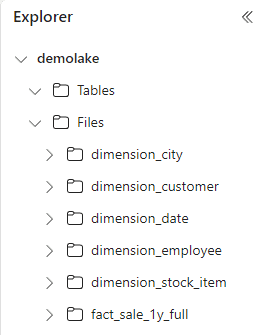
On the lake explorer, you will notice the folders for each table inside the Files area. The shows you that the data is ingested.
Interface gráfica do usuário Descrição gerada automaticamente

Ingest as Table

We ingested the data as binary files. Let’s analyse how would it be to ingest the data as a Table.

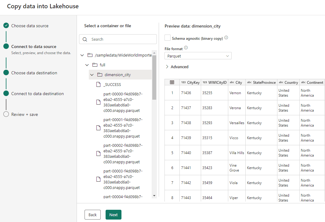
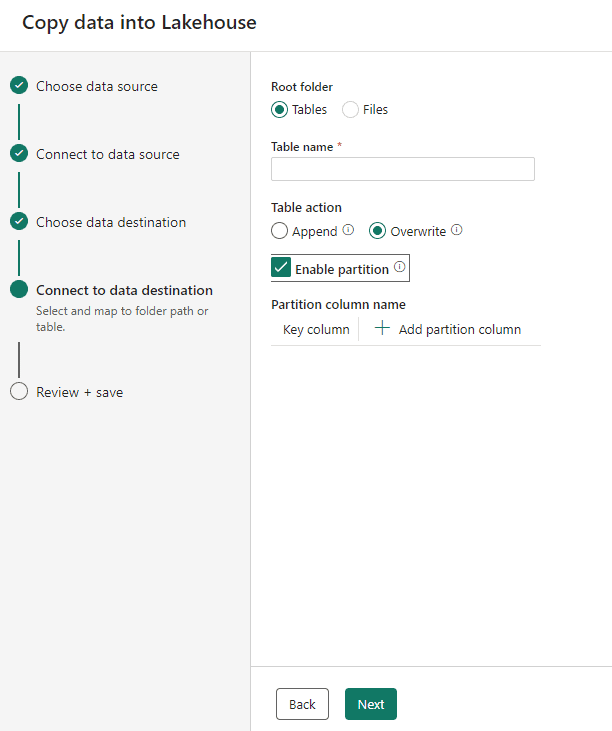
Back to selecting the source, during the Copy Data into Lakehouse wizard, if we select one single folder, which contains one single table, and select the correct data format, we can ingest the information to the Table area of the lakehouse.
Interface gráfica do usuário, Aplicativo Descrição gerada automaticamente

When selecting tables as destination, we can select the following options:

  • The table name
  • The Action: We can Append the data to an existing table or overwrite the data of an existing table.
  • Partitioning: All the storage is kept in Delta format. This format allows to partition the data according to field values. The partitioning will be done breaking the data in different folder. For example, if you choose to partition by Year, a different folder will be created for each year.
Interface gráfica do usuário, Aplicativo, Email Descrição gerada automaticamente

Files and Tables

The Files area in the lakehouse is dedicated to RAW data, the data just ingested. After the ingestion, we should load the data in the Tables area. The Tables area allow the following:

  • The data will be specially optimized, being able to reach a performance up to 10x the regular delta table performance.
  • The data is still 100% compatible with delta format.
  • The data is available for SQL Queries using the SQL Endpoint

Even if the data in the Files area is already in Delta format, the tables will only be available for the SQL Endpoint if converted to the Tables area.

There are two different methods to convert the data form the Files area to the Tables area: We can use the UI or we can use a spark notebook.

Missing Point

In tools such as Synapse Serverless, we can use SQL to access data from storage in many different formats using the OPENROWSET function. However, this feature is not available in Microsoft Fabric, at least yet.

Converting the Files into Tables

Let’s analyse some differences in relation to the usage of the UI and the usage of a spark notebook:

UI Conversion

Spark Notebook

No writing options configuration

Custom writing options configuration

No partitioning configuration

Custom partitioning configuration

Manual Process

Schedulable process

The process of conversion is very simple:

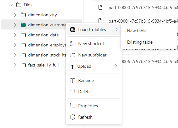
  • Right-Click the folder containing the files.
  • Select Load To Tables -> New Table

Interface gráfica do usuário, Aplicativo Descrição gerada automaticamente

The Existing Table option allow us to add more data in an existing table manually. However, the process will be too manual, it would be better to schedule a notebook for this.

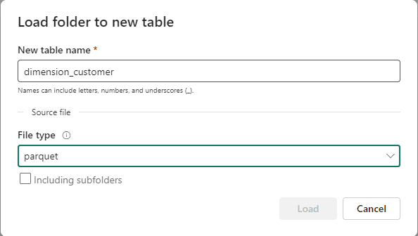
  • On the Load new folder to table window, type the name of the table in the New table name textbox
  • On the File type drop down, select parquet
Interface gráfica do usuário, Texto, Aplicativo, Email

  • Repeat the steps 21-24 for each table
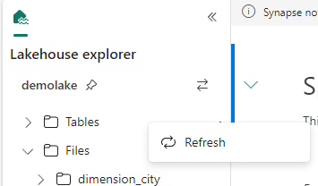
  • On the lakehouse explorer, right click Tables and click Refresh.
Interface gráfica do usuário, Aplicativo Descrição gerada automaticamente

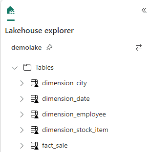
  • The tables are now available in the Tables area.
Interface gráfica do usuário, Aplicativo Descrição gerada automaticamente

  • On the left bar, click the demolake button.

Let’s look on the storage behind the tables in the lakehouse.

  • Right click the fact_sale table
  • On the context menu, click View files menu item.
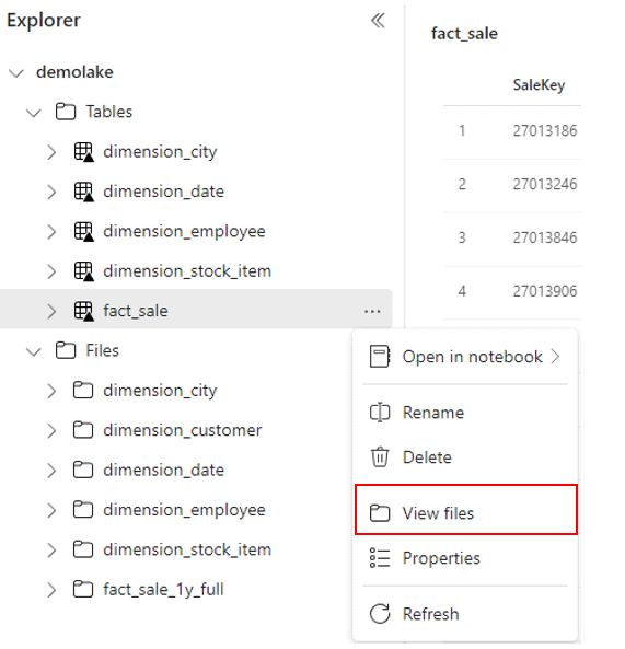
Interface gráfica do usuário, Aplicativo Descrição gerada automaticamente

Mind how the files are stored in delta format.
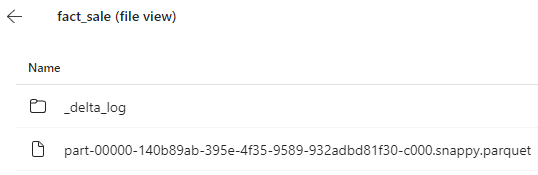
Interface gráfica do usuário, Texto, Aplicativo Descrição gerada automaticamente

Using a SQL Endpoint

The lakehouse provides a SQL Endpoint which allow us to use SQL language over the data.

Let’s make some experiments with the SQL Endpoint. We can use the box on the top right of the window to change the view from the lakehouse to the SQL Endpoint.
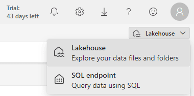
Interface gráfica do usuário, Texto, Aplicativo, chat ou mensagem de texto Descrição gerada automaticamente

The SQL Endpoint changes the Explorer view to a database format, showing only the Tables content as a database.
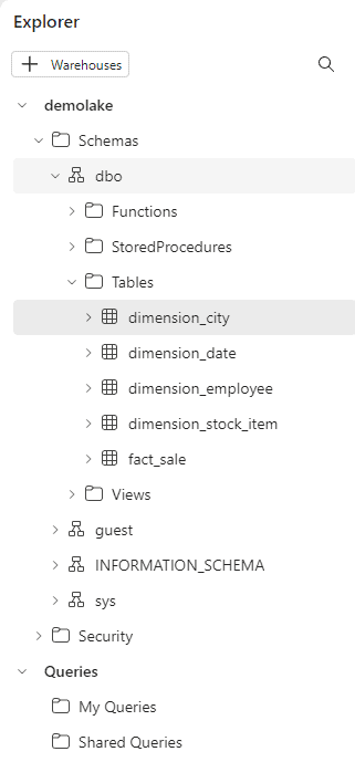
Interface gráfica do usuário, Texto, Aplicativo Descrição gerada automaticamente

On this view, we have the option to create queries, either SQL Queries or Visual Queries. The capability to create queries is available in many different places in Power BI and Microsoft Fabric environment:

Power BI Datamarts

I wrote about them and query creation here (https://www.red-gate.com/simple-talk/databases/sql-server/bi-sql-server/datamarts-and-exploratory-analysis-using-power-bi/) when the UI was still Design Tab and SQL Tab. The UI is slightly different today, but the meaning is the same – query creation, with two types of queries.

Fabric Data Warehouse

I wrote about it here (https://www.red-gate.com/simple-talk/blogs/microsoft-fabric-data-warehouse-ingestion-using-t-sql-and-more/) at that point, I only wrote about using the SQL Queries to execute DDL statements.

This is, in fact, one of the differences between a Data Warehouse and a SQL Endpoint: The Data Warehouse has full DDL support, while the SQL Endpoint has limited DLL support.

Fabric Lakehouse

This is the example illustrated on this article.

Am I missing other places where the same UI was implemented? Probably. Add on the comments, please.

Creating a Visual Query

  • Click the New Visual Query button.
  • Drag the Fact_Sale table to the Visual Query area.
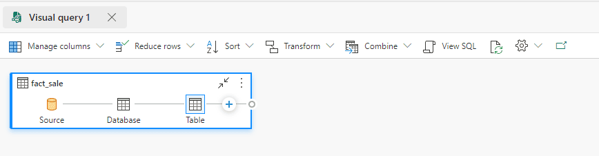
Interface gráfica do usuário, Texto Descrição gerada automaticamente com confiança média

  • Drag the Dimension_Customer table to the Visual Query area.
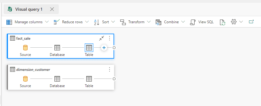
Interface gráfica do usuário, Texto, Aplicativo, Email Descrição gerada automaticamente

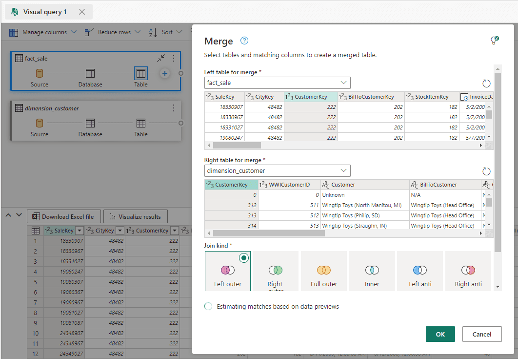
  • Click the + button on Fact_Sale in the Visual Query area and select Merge queries as new
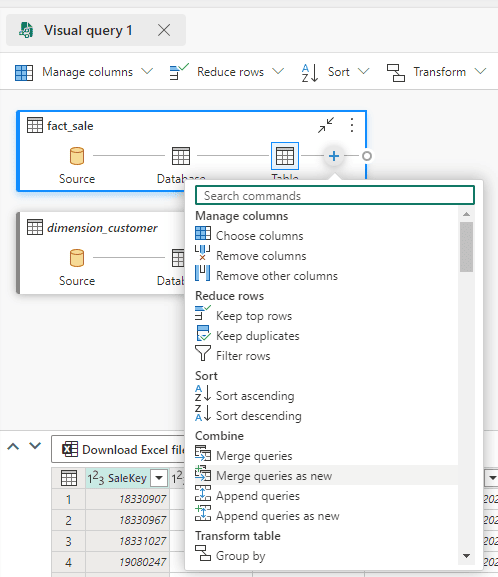
Interface gráfica do usuário, Aplicativo Descrição gerada automaticamente

  • Select the Dimension_Customer table on the Right table for merge drop down.

Interface gráfica do usuário, Tabela Descrição gerada automaticamente

  • Click the Ok button.
  • Click on the Data Display area and move the focus to the last column on the right.
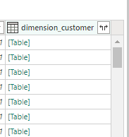
    Tabela Descrição gerada automaticamente

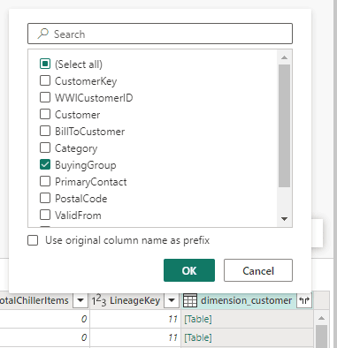
  • Click the Expand button and select only the BuyingGroup column.

   Interface gráfica do usuário, Aplicativo Descrição gerada automaticamente

After making a join between the tables, the columns from the first table are kept and we choose which columns from the second table we would like to include in the join as well.

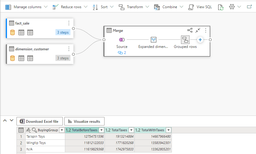
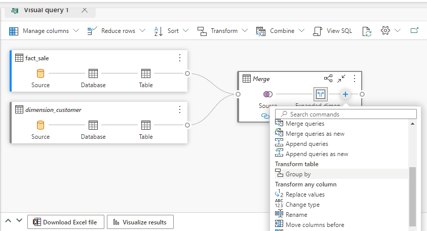
  • Click the + button on the merged table and select Group By
    Interface gráfica do usuário Descrição gerada automaticamente com confiança média 

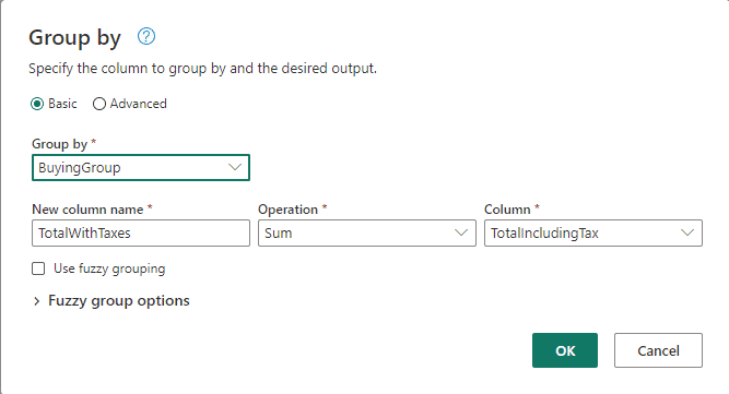
  • On the Group By window, Select BuyingGroup field in the Group By dropdown.
  • On the New column name textbox type TotalWithTaxes
  • On the Operation dropdown, select Sum.
  • On Column dropdown, select TotalIncludingTax field.

We have only used the Basic option on this example. The Advanced option would allow us to add multiple grouping fields and multiple aggregations.
A screenshot of a computer Description automatically generated

  • Click the Ok button.

Interface gráfica do usuário Descrição gerada automaticamente

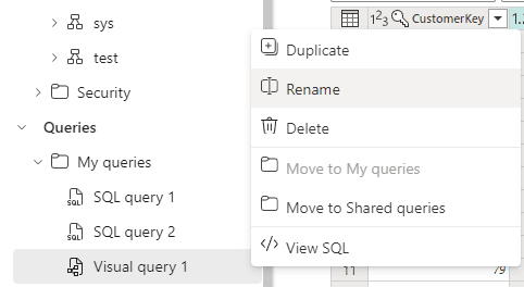
  • On the left window, under My Queries, click the expand .. button close the Visual Query 1 and select Rename.
Interface gráfica do usuário, Aplicativo Descrição gerada automaticamente

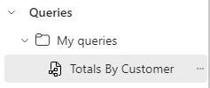
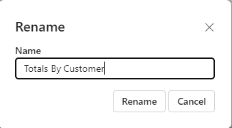
  • On the Rename window, on the Name textbox, type Totals By Customer
Interface gráfica do usuário, Texto, Aplicativo Descrição gerada automaticamente

  • Click the Rename button.

    Interface gráfica do usuário, Texto, Aplicativo Descrição gerada automaticamente

What to do with the queries

After creating a visual query, we can use it in many ways:

  • We can click the View SQL button and use the SQL to create a view or a materialized object.

At the time of publishing this article, the preview version has a bug and only shows the initial SQL query, not the final query with all the transformations. We hope this is fixed soon.
Interface gráfica do usuário, Aplicativo Descrição gerada automaticamente

  • We can download an excel file and continue our exploration on the Excel file.

The Excel is dynamically configured to execute the query against the Lakehouse. As a result, the data is dynamically load from the lake every time we open the Excel. We can save this file and use it to analyse the same query as many times as we would like.

These are the steps to download and use an Excel file:

  1. Click the Download Excel File button on the Display area.

  • Open the downloaded excel file.
  • Click the Enable Editing button.

This first warning is caused because the Excel file was downloaded from the web. This is the first level of security.

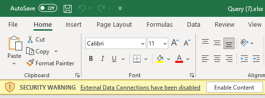
  • On the Security Warning, click Enable Content button.
A screenshot of a computer Description automatically generated

The Excel file opened contains dynamic content, including a SQL query to build an Excel table. This is active content which needs to be enabled. This is the 2nd level of security.

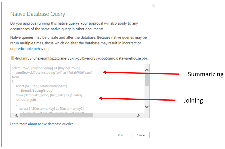
  • On the Native Database Query window, click the Run button.
A screenshot of a computer Description automatically generated

We will be running a SQL query pointing to a server. Excel shows the query and asks for confirmation. This is the 3rd level of security.

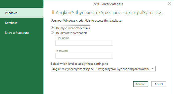
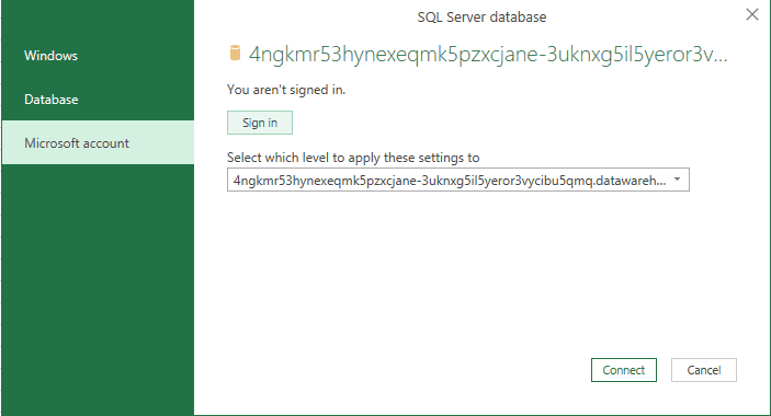
  • On the SQL Server Database window, choose Microsoft Account on the left side.
A screenshot of a computer Description automatically generated

  • Click the Sign In button and login with your Microsoft Fabric account.
A screenshot of a computer Description automatically generated

Mind the SQL Server address on this window: It’s in fact the SQL Endpoint address from the lakehouse.

  • Click the Connect button.

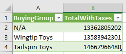
The SQL query will only be executed if the user opening the Excel file has permissions on the Microsoft Fabric SQL Endpoint. This is the 4th level of security.
A screenshot of a computer Description automatically generated

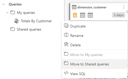
  • We can turn the query into a shared query and allow other team members to continue the data exploration.

On the context menu for the query, we choose Move to Shared Queries. We can move back to My Queries if we would like so.

There are only these two options: Or the query is private to the user, or it’s accessible to every user who has access to the lakehouse.
A screenshot of a computer Description automatically generated

Modelling the Tables

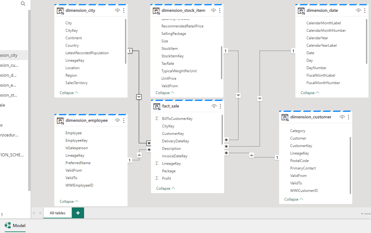
The SQL Endpoint in a lakehouse allow us to model the tables in the same way it does in a Data Warehouse and I illustrated on my article about Data Warehouse.

In the same way, the model is stored in the default dataset. By doing so, we establish a default modelling we would like the consumers to have when accessing the lakehouse. This is not only about table relationships, but also the creation of measures.
A screenshot of a computer Description automatically generated

Creating a Report

I already explained the process of building a report on my article about Data Warehouse, it’s very similar. I will approach details about the access from Power BI to OneLake in future articles.

The only difference worth mentioning on this point is that clicking on the button Visualize Results will create a dataset and a report from the query we visually generated. We can download and inspect the resulting dataset. It’s built with a single SQL query towards the lakehouse SQL Endpoint.

A white rectangular object with colorful text

Summary

Microsoft Fabric is a great tool, as I highlighted on my overview. It provides plenty of options about how to manage our data, either using a Data Warehouse, explained in a previous article, or a lake house, explained on this article. All the options linked by a common environment, the Power BI, going way beyond the BI area.

In future articles I will approach how to choose the option to use and how to organize these scenarios on an enterprise level.


The post Microsoft Fabric: Lakehouse and Data Factory in Power BI environment appeared first on Simple Talk.


from Simple Talk https://ift.tt/3HecR42
via

Tuesday, September 5, 2023

Orchestrating a MySQL Container on Kubernetes

If you’ve been using MySQL for a while and want to learn how to orchestrate MySQL containers, you’ve come to the right place. And while using Docker on its own to manage a single MySQL instance or multiple instances has certain drawbacks, such as lacking the ability to orchestrate multiple instances, scale, and provide services for external clients, in this blog we’ll explore how Kubernetes addresses these limitations and what to do when you’re facing problems.

To begin, visit the Docker Hub, find a Docker image called “mysql” (it can be utilized to generate a Docker container with a MySQL database instance on Kubernetes), and let’s begin.

Prerequisites

To follow along with this tutorial, you need the following:

  • Minikube and VirtualBox installed locally – This tutorial uses Minikube v1.25.2 and VirtualBox 6.1.
  • Basic knowledge of Kubernetes
  • Basic knowledge of MySQL

Setting up minikube

Minikube is a popular tool used in the development of Kubernetes-based applications. It allows developers to create a local Kubernetes cluster for testing, debugging, and experimenting with Kubernetes features and applications. To use Minikube, a virtualization driver is needed. The driver creates and manages a virtual machine that hosts the Kubernetes cluster. This tutorial uses VirtualBox as the driver, which is free and open-source virtualization software that allows users to run multiple operating systems on a single machine.

To create a Kubernetes cluster with Minikube and VirtualBox, you need to run the command:

minikube start --driver=virtualbox

This command will initiate MiniKube with VirtualBox as its driver. At present, VirtualBox is the most stable driver available for Minikube.

Set up MySQL on Kubernetes

Now we will set up MySQL – we will use a version of MySQL available on Docker Hub, authenticate it with credentials we’ll help you set up, and then create a pod. We will also create a PersistentVolume (PV) and PersistentVolumeClaim (PVC) to work with storage inside your Kubernetes Cluster. PV sets aside storage resources in the cluster for MySQL, while PVC requests storage from the PV.

To get started, you need to create a folder for all the Kubernetes YAML files. You will create the YAML file (my-storage.yaml) for storage first, which will include data for the PV and PVC, then paste the following code in it:

apiVersion: v1
kind: PersistentVolume
metadata:
   name: mysql-pv
spec:
   capacity:
      storage: 250Mi
   accessModes:
      - ReadWriteOnce
   hostPath:
      path: "/var/lib/mysql"
---
apiVersion: v1
kind: PersistentVolumeClaim
metadata:
    name: mysql-pv-claim
spec:
    accessModes:
        - ReadWriteOnce
    resources:
       requests:
          storage: 250Mi

The PersistentVolume resource, named mysql-pv, defines a storage volume with a capacity of 250Mi (250 megabytes) and is using the hostPath volume plugin, which allows the volume to be mounted from a file or directory on the host system. In this case, the volume is being mounted from the /var/lib/mysql directory on the host system, but make sure to change the path if you’ve set a different directory for your MySQL data files.

The PersistentVolumeClaim resource, named mysql-pv-claim, defines a request for a persistent volume with a capacity of 250Mi that can be mounted with read-write access by a single node at a time. This claim can then be used by other Kubernetes resources, such as a Deployment, to request storage resources.

Now send the above configuration to Kubernetes with the following command:

kubectl apply -f my-storage.yaml

After you’ve applied the configuration to Kubernetes, it’s time to move on to the deployment and the service.

Starting the Deployment and Service

Now, we’ll create the deployment and the service for MySQL. Kubernetes will pull the Docker image mysql:latest from Docker Hub and use it to create a container that will run on Kubernetes. In Kubernetes, a Service provides a stable IP address for a set of Pods, allowing other parts of the application to easily access the Pods without needing to know their specific IP addresses or ports and since your MySQL image will require the values of the variables named MYSQL_ROOT_PASSWORD, MYSQL_DATABASE, MYSQL_USER and MYSQL_PASSWORD, we will need to create those secret values before deployment.

You can create these values by running the following commands (replace put-database-name, put-root-password, put-username, and put-user-password with values relevant to your database.) Also keep in mind that in Kubernetes, a secret may also contain more than one key/value pair:

kubectl create secret generic mysql-db --from-literal=database=put-database-name

kubectl create secret generic mysql-root-pass --from-literal=password=put-root-password

kubectl create secret generic mysql-user-pass --from-literal=username=putusername --from-literal=password=put-user-password

Here, the Kubernetes manifest creates a Service resource named “mysql” that exposes a port (3306) on the nodes in the cluster via a NodePort. The selector specified in the manifest ensures that the Service routes traffic to pods with the label app: mysql.

To get the deployment and Service going, create a new manifest file (mysql.yaml) and paste in the following code.

apiVersion: v1
kind: Service
metadata:
   name: mysql
spec:
   type: NodePort
   selector:
      app: mysql
   ports:
      - port: 3306
      targetPort: 3306
      nodePort: 30007
---
apiVersion: apps/v1
kind: Deployment
metadata:
   name: mysql-deployment
   labels:
      app: mysql
spec:
   replicas: 1
   selector:
      matchLabels:
         app: mysql
   template:
      metadata:
         labels:
            app: mysql
      spec:
         volumes:
         - name: mysql-pv
           persistentVolumeClaim:
              claimName: mysql-pv-claim
      containers:
        - name: mysql
          image: mysql:latest
          env:
          - name: MYSQL_ROOT_PASSWORD
            valueFrom:
               secretKeyRef:
                  name: mysql-root-pass
                  key: password
          - name: MYSQL_DATABASE
            valueFrom:
               secretKeyRef:
                 name: mysql-db
                 key: database
          - name: MYSQL_USER
            valueFrom:
               secretKeyRef:
                 name: mysql-user-pass
                 key: username
          - name: MYSQL_PASSWORD
            valueFrom:
               secretKeyRef:
                 name: mysql-user-pass
                 key: password
            volumeMounts:
          - name: mysql-pv
            mountPath: /var/lib/mysql
            ports:
            - containerPort: 3306
              name: mysql

Explanation of the code above:

Here’s what you need to know about the code block you’ve just reviewed:

  • spec: This section contains the specifications for the Kubernetes resource, such as the type of Service or the number of replicas for the Deployment.
  • selector: This section specifies the label selector for the Service or Deployment. In this case, the Service will match pods with the app=mysql label and the Deployment will select pods with the app=mysql label.
  • type: This section specifies the type of Service being created. In this case, the type is NodePort, which exposes the Service on a static port on each node in the cluster.
  • ports: This section specifies the ports that the Service will listen on. In this case, the Service will listen on port 3306 and forward traffic to port 3306 on the pods.
  • volumes: This section specifies the volumes that will be used by the container. In this case, there is one volume named mysql-pv, which is created by a PersistentVolume.
  • containers: This section specifies the containers that will be run by the Deployment. In this case, there is one container named mysql, which is using the mysql:latest Docker image.
  • env: This section specifies the environment variables that will be set for the container. In this case, there are four environment variables being set using secrets created from Kubernetes Secret resources. This was set earlier.
  • volumeMounts: This section specifies the mount points for the volumes that will be used by the container. In this case, there is one volume named mysql-pv, which is mounted to the container’s /var/lib/mysql directory.
  • containerPort: This section specifies the port that the container will listen on. In this case, the container will listen on port 3306.

Now, apply your configuration by running the command below:

kubectl apply -f mysql.yaml

This command applies a configuration to a resource from a given file. Let Kubernetes do its thing and after 5-10 minutes, run the following command to check if your pod is running the following command. Take note of the pod name – you will need it to interact with your database later on.

kubectl get pods

If your pod is running, you should see something like the image below:

In this section, we have been able to create a pod where the MySQL server will run. We will need this is the next sections to work on the server.

Interacting with the Database

Now, we will start an interactive shell to interact with our MySQL database. The interactive shell will enable us to interact with MySQL through the CLI. Start the interactive shell by running the following command (replace paste-pod-name with the name of the pod you’ve just taken note of):

kubectl exec --stdin --tty paste-pod-name -- /bin/bash

Within the interactive shell, run the following command to start the MySQL CLI as the root user (username you created earlier). You will be prompted to provide the password. Provide the password you used in this command:

kubectl create secret generic mysql-root-pass --from-literal=password=put-root-password

This command was used to store the root password.

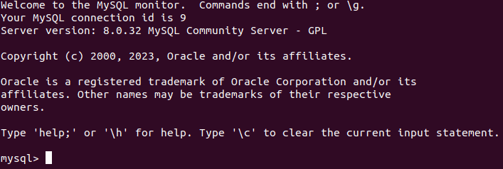
Now, log in to your MySQL instance – provide a username and a password:

mysql –u [putusername] –p

Your result should look like the image below.

Now run the following command to create a new database:

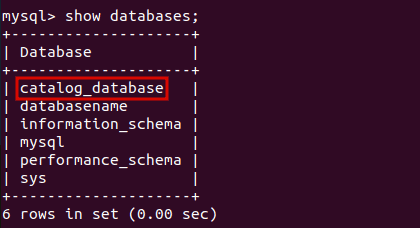
CREATE DATABASE catalog_database;

Now run the following MySQL command to list the databases available, and you should see all your databases including the one you just created.

show databases;

Now navigate into any of your databases with the following command:

use catalog_database;

Next, create a database table called Catalog with the following SQL statement.

CREATE TABLE Catalog(
  CatalogId INTEGER PRIMARY KEY,
  Journal VARCHAR(25),
  Publisher VARCHAR(25),
  Edition VARCHAR(25),
  Title VARCHAR(45),
  Author VARCHAR(25)
);

Add a row of data to the Catalog table with the following SQL statement.

INSERT INTO Catalog 
VALUES('1','Muscle Magazine','Jude Mag', 'June 2013',
       'How to grow muscles','Muhammed Ali');

The Catalog table gets created and a row of data gets added. You can checkout your data with the following statement:

SELECT * 
FROM Catalog;

Conclusion

In this article, we learned how to orchestrate the MySQL database using Kubernetes. We started with specifying the storage specification for the database, then moved to creating the deployment that runs the MySQL container. We also created a Kubernetes service so that the database can be accessed. Furthermore, we went further to interact with the database running in Kubernetes.

Now, in the unlikely event of a database failure, a new instance will automatically be generated for you, ensuring that all your data remains intact and persistent.


The post Orchestrating a MySQL Container on Kubernetes appeared first on Simple Talk.


from Simple Talk https://ift.tt/3zCn2MY
via

Monday, September 4, 2023

SQL Server Row Level Security Deep Dive. Part 2 – Setup and Examples

The previous section in this series was an introduction to Row Level Security (RLS) and some use cases. This section focuses on basic setup of RLS, methods for implementing RLS and performance considerations with those implementations. The RLS access predicate is applied to every row returned to a client making performance a big factor in any design. Expensive lookups or other bad designs can hurt not only performance on that table but overall system performance if CPU or IO is heavily impacted.

Basics

Define the strategy based on business requirements

Implementing RLS is as much a business endeavour as technical. Without a business case to implement RLS, there is no reason for the extra effort and testing involved. This is where driving out business requirements and making sure the solution fits the problem is important. Non-technical members of the team or business partners likely won’t know what RLS is or if it should be used. Differential access to the same data, replacing systems (or proposed systems) with multiple reports based on user groups, and multi-tenant access are possible indicators that RLS may be a useful tool. There are always multiple ways to solve a problem. If RLS would simplify the design and make it more robust, that’s when I start to seriously consider it for a design. It does help if the business is aware of RLS and have used it in other projects or databases, but having the business essentially design the system is dangerous too. Use all of the information available during planning sessions and design the system that best fits the need of the business and the skills of the technical team.

The business requirements should include a method to determine the rows allowed based on groups of users. It can be a very broad definition, such as country or business division assigned to a user, or it can much more specific and elaborate. Whatever method is decided, there should be an automated method to enable that strategy in the database for each user. The method can be active directory groups or properties, SQL roles, application database tables, a front-end designed and coded for this purpose (in conjunction with configuration tables), or any other method determined by the business. The strategy needs to be translated to something accessible to the database engine. Several methods are listed in the official documentation and are discussed below, but the actual authorization groups used by the RLS access predicate will likely be stored in the SESSION_CONTEXT, a lookup table, or a SQL role.

An access predicate is defined for each table

The actual implementation of RLS happens with two database objects, an access predicate and a security policy. The access predicate is an inline table-valued function (TVF) and defines the authorization and lookup process. This table-valued function is applied to each row that would be returned to the user. It is evaluated and only allows the row to return if the defined criteria are met. This sounds like a very general description, but that’s because it is very general. The rows returned are based on the business requirements defined for your project. Each RLS implementation is a custom solution and requires the rules to be implemented in the access predicate.

The access predicate defines the security mechanism for each row. Lookup queries and joins can be used, but they have a performance cost. The column used for security is passed in as a parameter and must be available in the table or the system (i.e., @CountryCode). Rows are then filtered (for read operations) or blocked (for write operations), or both. The filtering process is defined by the security policy.

A security policy is defined for each table

The security policy is what ties the access predicate to the table, specifies the column to be used as the parameter in the predicate, indicates how data should be restricted (filter, block, or both), and if RLS is enabled for the table or not via the STATE value. It is the mechanism that enables or disables RLS at a table level. Remember that RLS is table specific and only applies to tables where it is applied. That’s the job of the security policy. Each table can have a maximum of 1 security policy assigned. It can be enabled for both options, filter and block, but only one policy can be on a table.

Examples

The following examples use the WideWorldImporters sample database. They show basic access predicates and security policies.

Example 1 – lookup table

The following example shows a lookup table getting used to perform the authorization process. This example uses a local table in a separate schema, RLS. This is more secure from a procedural standpoint since you can be sure that regular users don’t have access to the table and aren’t able to modify it as long as you don’t use db_datareader or db_datawriter.

CREATE SCHEMA RLS
AUTHORIZATION dbo
GO
--Create the table to hold the RLS rules
CREATE TABLE RLS.UsersSuppliers (
        UsersSuppliersID                int                             NOT NULL CONSTRAINT PK_RLSUsersSuppliers PRIMARY KEY CLUSTERED          identity
        ,UserID                                 nvarchar(255)   NOT NULL
        ,SupplierID                             int                             NOT NULL
)
GO
CREATE UNIQUE NONCLUSTERED INDEX UNQ_RLSUsersSuppliers_NaturalKey
ON RLS.UsersSuppliers (
        UserID
        ,SupplierID
)
GO
--Test user without a login
CREATE USER RLSLookupUser WITHOUT LOGIN
GO
--Grant SELECT access to the entire Purchasing schema
--Deny SELECT on the RLS schema
GRANT SELECT ON SCHEMA::Purchasing TO RLSLookupUser
DENY SELECT ON SCHEMA::RLS TO RLSLookupUser
GO
--Grant the test user access to a single supplier ID
INSERT INTO RLS.UsersSuppliers (
        UserID
        ,SupplierID
)
VALUES (
        'RLSLookupUser'
        ,4
)
GO
--Simple access predicate with a lookup
CREATE FUNCTION RLS.AccessPredicate_SupplierID_PurchasingSuppliers(@SupplierID  int)
RETURNS TABLE
WITH SCHEMABINDING
AS
RETURN
        SELECT 
                1 AccessResult
        FROM RLS.UsersSuppliers US
                INNER JOIN Purchasing.Suppliers PS
                        ON US.SupplierID        = PS.SupplierID
        WHERE US.SupplierID                     = @SupplierID
                AND US.UserID                   = USER_NAME()
GO
--Enforce the access predicate defined above
--Note that the STATE = ON
CREATE SECURITY POLICY RLS.SecurityPolicy_SupplierID_PurchasingSuppliers
ADD FILTER PREDICATE RLS.AccessPredicate_SupplierID_PurchasingSuppliers(SupplierID) ON Purchasing.Suppliers
,ADD BLOCK PREDICATE RLS.AccessPredicate_SupplierID_PurchasingSuppliers(SupplierID) ON Purchasing.Suppliers AFTER UPDATE
WITH (STATE = ON, SCHEMABINDING = ON)
GO

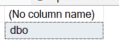
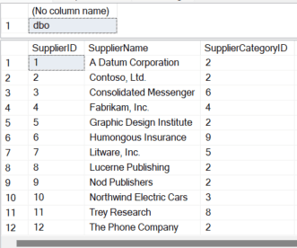
Be sure to validate your RLS configuration. The test user above, RLSLookupUser, is shown doing this below. Note that it was executed in the context of a dbo account and no rows are returned.

--Show the current user name
SELECT USER_NAME()
--Rows returned with RLS applied
SELECT *
FROM Purchasing.Suppliers

--Change the user running the SELECT
EXECUTE AS USER = 'RLSLookupUser'
SELECT *
FROM Purchasing.Suppliers
--Revert back to the logged in user
REVERT

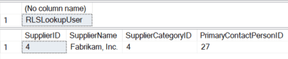
Notice that the SupplierID matches the ID in the script populating the RLS.UsersSuppliers table, 4.

Example 2 – lookup table with dbo override

This example differs in that it checks for the db_owner role. If found, all rows are returned. This is useful if it fits your use case. It makes it easier for DBAs to perform maintenance on the RLS tables and run ad-hoc statements to fix issues.

--Drop the security policy so the old access predicate has no references
DROP SECURITY POLICY RLS.SecurityPolicy_SupplierID_PurchasingSuppliers
--WITH (SCHEMABINDING=OFF)
GO
--Drop the old access predicate so the new one can be created
DROP FUNCTION  RLS.AccessPredicate_SupplierID_PurchasingSuppliers
GO
CREATE FUNCTION RLS.AccessPredicate_SupplierID_PurchasingSuppliers(@SupplierID  int)
RETURNS TABLE
WITH SCHEMABINDING
AS
RETURN
        SELECT 1 AccessResult
        WHERE IS_MEMBER('db_owner') = 1 
        UNION
        SELECT 
                1 AccessResult
        FROM RLS.UsersSuppliers US
                INNER JOIN Purchasing.Suppliers PS
                        ON US.SupplierID        = PS.SupplierID
        WHERE US.SupplierID                     = @SupplierID
                AND US.UserID                   = USER_NAME()
GO
--Enforce the access predicate defined above
--The same security policy is used
CREATE SECURITY POLICY RLS.SecurityPolicy_SupplierID_PurchasingSuppliers
ADD FILTER PREDICATE RLS.AccessPredicate_SupplierID_PurchasingSuppliers(SupplierID) ON Purchasing.Suppliers
,ADD BLOCK PREDICATE RLS.AccessPredicate_SupplierID_PurchasingSuppliers(SupplierID) ON Purchasing.Suppliers AFTER UPDATE
WITH (STATE = ON, SCHEMABINDING = ON)
GO

Note that a UNION is used rather than an OR in the WHERE clause. This is a general tuning guideline and usually works better for all queries, not just RLS access predicates. Notice how running the SELECT as a dbo returns all rows, but the first user is still restricted.

--Show the current user name
SELECT USER_NAME()
--Rows returned with RLS applied
SELECT *
FROM Purchasing.Suppliers
--Change the user running the SELECT
EXECUTE AS USER = 'RLSLookupUser'
SELECT USER_NAME()
SELECT *
FROM Purchasing.Suppliers
--Revert back to the logged in user
REVERT

In contrast to the first example, all rows are returned for the dbo account.

Example 3 – Role member lookup

The next example is similar to the method used in the base implementation of the WideWorldImporters sample database. It has a dbo override and also checks for role membership.

--Create a role for each customer type
CREATE ROLE [CustomerType_Agent]
CREATE ROLE [CustomerType_Wholesaler]
CREATE ROLE [CustomerType_Novelty Shop]
CREATE ROLE [CustomerType_Supermarket]
CREATE ROLE [CustomerType_Computer Store]
CREATE ROLE [CustomerType_Gift Store]
CREATE ROLE [CustomerType_Corporate]
CREATE ROLE [CustomerType_General Retailer]
--The Gift Store type has associated records so it is used for this example
--All other types would have an associated user or you could
--assign a group or specific users to the various roles
CREATE USER RLSGiftStore WITHOUT LOGIN
GO
ALTER ROLE [CustomerType_Gift Store] ADD MEMBER RLSGiftStore
GO
ALTER ROLE db_datareader ADD MEMBER RLSGiftStore
GO
--Add the access predicate. 
--This shows two things
--1. The Lookup based on role member using the IS_ROLEMEMBER function
--2. The JOIN to the CustomerCategories table. This is not a direct lookup for the base RLS table
CREATE FUNCTION RLS.AccessPredicate_CustomerID_SalesCustomers(@CustomerID       int)
RETURNS TABLE
WITH SCHEMABINDING
AS
RETURN
        SELECT 1 AccessResult
        WHERE IS_MEMBER('db_owner') = 1 
        UNION
        SELECT ISNULL(AccessResult,0)
        FROM (
                        SELECT 
                1 AS AccessResult
        FROM Sales.Customers C
                INNER JOIN Sales.CustomerCategories CC
                        ON C.CustomerCategoryID         = CC.CustomerCategoryID
        WHERE C.CustomerID                                      = @CustomerID
                AND IS_ROLEMEMBER(N'CustomerType_' + CC.CustomerCategoryName,USER_NAME())               = 1) AccessPredicate
GO
--Add the security policy
--This is straight forward, but also note that it uses the CustomerID
--and not the CustomerCategoryName. The name is a lookup in CustomerCategories
CREATE SECURITY POLICY RLS.SecurityPolicy_CustomerID_SalesCustomers
ADD FILTER PREDICATE RLS.AccessPredicate_CustomerID_SalesCustomers(CustomerID) ON Sales.Customers
,ADD BLOCK PREDICATE RLS.AccessPredicate_CustomerID_SalesCustomers(CustomerID) ON Sales.Customers AFTER UPDATE
WITH (STATE = ON, SCHEMABINDING = ON)
GO

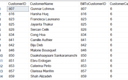
This only returns 50 rows out of the 663, which is correct based on RLS rules.

EXECUTE AS USER = 'RLSGiftStore'
SELECT *
FROM Sales.Customers
REVERT
GO

As you can see, implementing RLS is relatively simple once you understand how everything is connected. Keeping it simple is important for maintenance and performance.

Authorization methods in RLS

The authorization method for RLS involves storing user information in a table or using another lookup strategy. The examples above show a lookup table and role membership for granting access, but any lookup can be used. This needs to defined after the business rules are determined and it is directly tied to that analysis. This storage or lookup strategy will determine how the access predicate functions. Complex methods will likely benefit with being stored in a table. This is also useful when users are allowed to directly query data themselves. When all access is managed through an application, SESSION_CONTEXT is a viable solution. It all depends on the business need, the current technical solutions in place, and the method that will be used to access the RLS protected data.

CONTEXT_INFO()

It is possible to use CONTEXT_INFO for RLS, but this is definitely not recommended. It is a clear security risk since any user can override their own information. It is also not possible to lock these values when they are set. In simple terms, it means a user can change or set RLS security if it uses CONTEXT_INFO. Do not use CONTEXT_INFO for RLS.

SESSION_CONTEXT()

SESSION_CONTEXT can be used for RLS and it is a secure solution when implemented correctly. SESSION_CONTEXT works with all versions of SQL, including Azure SQL Database and with Microsoft Fabric. The key to making SESSION_CONTEXT secure is setting the value to read only when it is created.

The following has a potential security gap:

EXEC sp_set_session_context 'RLSRegion', 'Central'

That gap is closed by using the syntax below. The last parameter, 1, is for the @read_only parameter:

EXEC sp_set_session_context 'RLSRegion', 'Central', 1

If a user tries to override the value after it has been set, they will get the following error. If the user opens a new session, SESSION_CONTEXT is not set, meaning a user could set it to any value.

The other crucial part is ensuring that the SESSION_CONTEXT is set for each user. If access is only allowed through an application, it is relatively easy to be sure it is set. If the SESSION_CONTEXT is not set, the user won’t have access. This is also a security gap if the user can run commands since they will be able to set it themselves to any value.

A logon trigger can be used for full instances of SQL Server, on-prem and managed instances in Azure. If implemented, it needs to be very lightweight without a complicated lookup. This will be run for every connection to the server, so it may not work well for servers supporting multiple applications and databases. Thorough testing is recommended.

Local lookup table / Synapse lookup table

Storing authorization groups in a table works well for very complex authorization groups, such as multiple tiers of access (i.e., city, state, country, region). Complex RLS schemes don’t work well during the query process unless they are simplified. In my example of city, state, country, region, it works better to store each city allowed by the user, even if they are assigned access at a higher level (i.e., country). This might result in thousands of rows for a single user in the RLS table, but a very fast lookup process and it eliminates multiple joins in the access predicate. This assumes proper indexes on both the tables protected by RLS and the authorization table. Even with this general recommendation, it is always good to test your specific scenario. It is always possible to take things to an extreme level that doesn’t work well. If it is difficult or not possible to expand a hierarchy, care must be taken in the access predicate to ensure performance is acceptable. Normal query performance guidelines should be followed. It is usually better to include a UNION statement, or multiple UNION statements, rather than using OR statements in a JOIN.

Storing the authorization groups in a table also works well when users are allowed to query data directly or when multiple tools or applications are allowed to hit a warehouse and it isn’t feasible to create separate views and stored procedures for each group. In other words, ad-hoc queries from the perspective of the query engine. It is much more difficult to force the SESSION_CONTEXT to be set for every connection in an ad-hoc scenario. Setting the SESSION_CONTEXT can be done with SQL Server or in an Azure managed instance with a logon trigger, but this is not supported in Azure SQL Database. If that is your environment or in your upgrade path, it isn’t an option and you will want to look at a table-based solution instead.

This will be revisited during the section dedicated to security mitigations, but there are a few things to keep in mind if storing RLS authorization groups in tables. Put the lookup table and any tables used to support the lookup table in a separate scheme inaccessible to regular users (the RLS schema in my examples above). Update rights should be very limited. This also means that built-in database roles shouldn’t be used for regular users either, including the usual db_datareader and db_datawriter.

SQL Roles

SQL Roles can be used as a lookup mechanism in access predicates. Simple lookups would work well with this pattern. Since active directory groups can also be members of roles, that makes a good pattern and is easy to maintain. The sample in WideWorldImporters uses this as one of several methods for lookups.

SELECT 1 AS AccessResult
        WHERE IS_ROLEMEMBER(N'db_owner') <> 0

Specific users

Specific users can also be targeted by access predicates. This may be a good method to ensure that your administrator account always has access. It can also be used in conjunction with other lookups. This method is also demonstrated in the WideWorldImporters sample.

ORIGINAL_LOGIN() = N'Website'

Staging tables

A common pattern for warehouses is to create staging tables where raw or partially processed data can be placed before it is fully curated and made generally available to end users. If this pattern is used, be sure to put the staging tables in a different database or separate schema. This segregated space should not be accessible by regular users, even for SELECT access. Consider using the DENY permission on the ETL schema in addition to not granting permission to the schema if the tables are in the same database as the processed tables. In large organizations it is easy for a security request to be granted inadvertently if it follows patterns for standard databases but shouldn’t be followed in your RLS enabled database.

Summary

Creating and setting up RLS is relatively easy once the business rules are clearly understood. It may be necessary to create and regularly populate configuration tables for this process or add other structures to the database, such as user roles. A single access point and security predicate is then added to a table for RLS to be enabled. There are a number of methods to perform the lookup, including local tables, SESSION_CONTEXT() or any other method that meets the business need. Keep security and performance in mind at each stage of design. Each method implementing RLS has potential security holes and potential performance issues. Testing and validation of each method is key to any RLS setup.

Next sections on RLS:

Part 3 – Performance and Troubleshooting

Part 4 – Integration, Antipatterns, and Alternatives to RLS

Part 5 – RLS Attacks

Part 6 – Mitigations to RLS Attacks

Reference

https://learn.microsoft.com/en-us/sql/t-sql/functions/session-context-transact-sql?view=sql-server-ver16

https://learn.microsoft.com/en-us/sql/relational-databases/triggers/logon-triggers?view=sql-server-ver16

https://learn.microsoft.com/en-us/sql/relational-databases/system-stored-procedures/sp-set-session-context-transact-sql?view=sql-server-ver16

https://learn.microsoft.com/en-us/sql/relational-databases/security/row-level-security?view=sql-server-ver16

The post SQL Server Row Level Security Deep Dive. Part 2 – Setup and Examples appeared first on Simple Talk.


from Simple Talk https://ift.tt/vgyCfP6
via

Friday, September 1, 2023

Decoding Efficiency in Deep Learning, A Guide to Neural Network Pruning in Big Data Mining

In recent years, deep learning has emerged as a powerful tool for deriving valuable insights from large volumes of data, more commonly referred to as big data. Harnessing the computational capabilities of artificial neural networks, deep learning algorithms have the ability to model complex patterns and make accurate predictions based on these patterns. This makes them particularly valuable in big data mining, a field that deals with extracting meaningful information from substantial datasets.

However, as much as deep learning presents numerous opportunities for big data mining, it also brings forth significant challenges. One of the critical issues is inefficiency, especially in the context of large-scale deep learning networks. These networks often comprise millions, if not billions, of parameters that demand high computational power and substantial time for training. The resources required scale dramatically with the size of the data being processed, which can be a significant barrier to efficient big data mining.

To tackle this issue, various strategies have been developed, one of the most effective being neural network pruning. This process involves systematically eliminating the less important neurons or connections within a network, thereby reducing its complexity without significantly affecting its performance. By effectively “pruning” the network, we can dramatically enhance computational efficiency and reduce the resources needed for training and deployment. This article aims to provide a comprehensive guide to neural network pruning techniques, offering insights into how they can help enhance deep learning efficiency in big data mining.

Neural Network Pruning: An Overview

Think of a neural network as a complex machine with many adjustable knobs. Each of these knobs controls a particular aspect of the machine’s behavior. In the context of neural networks, these “knobs” are referred to as parameters, and they determine how the network processes information. For example, imagine a basic neural network designed to predict house prices. If you adjust a knob (or parameter) slightly, the network might start predicting slightly higher prices for houses with swimming pools. If you adjust another knob, it might give more importance to the size of the house. When we talk about “pruning” in neural networks, it’s like we are identifying which knobs are not contributing much to the machine’s accuracy and removing them. By doing so, we simplify our machine, making it faster and more efficient, without significantly compromising its ability to predict house prices accurately.

Neural network pruning is a process for optimizing a trained neural network by reducing the number of parameters or computational resources it uses, without significantly impacting its predictive performance. The idea is to “prune” away the less significant parts of the network, such as certain weights or neurons, effectively reducing the network’s complexity and size.

This technique is particularly effective in scenarios where you have a large, over-parameterized model that performs well but is too computationally expensive or large for the hardware you need to deploy it on. By removing parts of the network that contribute least to the output predictions, you can often create a smaller, faster model that still maintains a high level of accuracy.

Neural network pruning offers several advantages. It can:

  • Reduce the model’s memory footprint, making it possible to deploy larger models on devices with limited memory capacity.
  • Decrease the computational requirements, leading to faster predictions, which is especially crucial in real-time applications.
  • Lower energy consumption, which is essential for battery-powered devices.
  • Provide a level of regularization, which may reduce overfitting and improve the model’s ability to generalize from the training data to unseen data.

Principle of Neural Network Pruning

The fundamental principle behind neural network pruning is the idea that not all neurons in a network contribute equally to the output. Some connections (weights) between neurons have minimal influence on the final prediction of a network. By identifying and removing these connections, we can simplify the network without significantly degrading performance. This removal process, known as “pruning”, results in a “sparse” model with fewer parameters, leading to quicker inference and lower memory usage.

Two broad categories of pruning are “weight pruning” and “neuron pruning”. In weight pruning, we remove individual connections in the neural network, setting the corresponding weights to zero. This results in a sparse representation of weight matrices. On the other hand, in neuron pruning, we remove entire neurons along with their connections, which leads to a smaller, less complex network.

How Pruning Helps in Reducing Overfitting and Improving Model Generalization

Pruning has a regularizing effect on the neural network, helping prevent overfitting. Overfitting occurs when a model learns the training data too well, including its noise and outliers, resulting in poor performance on unseen data. By reducing the model’s complexity through pruning, we limit its capacity to memorize the training data, thereby enhancing its ability to generalize to new data.

Techniques of Neural Network Pruning

Neural network pruning techniques can be broadly categorized into four types: Weight Pruning, Neuron Pruning, Structured Pruning, and Sparse Pruning. These methods differ mainly in the scope and strategy of the pruning process.

Weight Pruning

Weight pruning involves eliminating the least important weights in the network, essentially setting these weights to zero. This results in a sparse representation of weight matrices, where the zero weights indicate pruned connections.

A simple method for weight pruning is magnitude-based pruning, where weights below a certain absolute magnitude are pruned. Here’s how you might implement it:

```python
def magnitude_pruning(model, pruning_percent):
    # Calculate the threshold value as the 
    #(pruning_percent)th percentile of the weight magnitudes
    all_weights = np.concatenate([np.abs(w.numpy().flatten()) 
                                       for w in model.weights])
    threshold = np.percentile(all_weights, pruning_percent)
    
    # Create a new model with the same architecture
    new_model = create_model()  # Assume create_model() 
            #returns a new model with the same architecture
    new_model.set_weights(model.get_weights())  # Copy weights        
                              #from the old model to the new one
    
    # Prune the weights
    for w in new_model.weights:
        w.assign(tf.where(tf.abs(w) < threshold, 0., w))
        
    return new_model
```

This function prunes the given percent of the smallest weights in the model and returns a new model with pruned weights.

Neuron Pruning

Neuron pruning is a more aggressive approach that involves removing entire neurons and their associated connections from the neural network. This results in a reduced model size and complexity. One common strategy is to prune neurons with the smallest L2-norm of weights in the outgoing layer.

def neuron_pruning(model, pruning_percent):
    # Calculate the L2 norm for each neuron in the layer
    norms = np.linalg.norm(model.layers[1].get_weights()[0], 
                                                       axis=0)
    
    # Determine the threshold for pruning
    threshold = np.percentile(norms, pruning_percent)
    
    # Create a mask for neurons to keep (non-pruned neurons)
    mask = norms >= threshold
    
    # Apply the mask to the weights and biases
    weights, biases = model.layers[1].get_weights()
    model.layers[1].set_weights([weights[:, mask], 
                                              biases[mask]])
    
    return model

Sparse Pruning

Sparse pruning aims at making the connections in the neural network sparse without changing the overall architecture. It’s similar to weight pruning but with the aim to achieve a certain level of sparsity in the model. This method is often used in combination with other pruning methods to achieve the desired level of sparsity.

# Define pruning parameters
pruning_params = {
      'pruning_schedule': 
              sparsity.PolynomialDecay(initial_sparsity=0.0,
              final_sparsity=0.9,  # aiming for 90% sparsity
              begin_step=0,
 end_step=10000)
}
# Apply the pruning wrapper to the model
pruned_model = 
     sparsity.prune_low_magnitude(model,**pruning_params)
#Now, compile and retrain the pruned model for a few epochs
pruned_model.compile(optimizer='adam', 
                loss='sparse_categorical_crossentropy',
                metrics=['accuracy'])
pruned_model.fit(x_train, y_train, epochs=5, 
                  validation_data=(x_test, y_test))
# After retraining, further prune the model
pruned_model = 
    sparsity.prune_low_magnitude(pruned_model, **pruning_params)
# ...and so on, until the desired level of sparsity is reached

Structured Pruning

Structured pruning involves removing structured sets of parameters or connections. (The previous methods are generally known as unstructured pruning methods.) For instance, pruning an entire filter from a convolutional layer, or pruning all weights associated with a specific feature map. This method can preserve the hardware efficiency of the pruned models, as certain hardware architectures are not optimized for handling sparsely connected layers.

def structured_pruning(model, pruning_percent):
    # Calculate the L2 norm for each filter in the convolutional layer
    norms = np.linalg.norm(model.layers[1].get_weights()[0], 
                                                 axis=(0, 1, 2))
    
    # Determine the threshold for pruning
    threshold = np.percentile(norms, pruning_percent)
    
    # Create a mask for filters to keep (non-pruned filters)
    mask = norms >= threshold
    
    # Apply the mask to the filters and biases
    filters, biases = model.layers[1].get_weights()
    model.layers[1].set_weights([filters[:,:,:,mask],
                                             biases[mask]])
    
    return model

Note

Each of these pruning techniques serves different purposes and is suited to different types of neural network architectures. The choice of technique depends on the specific requirements and constraints of the task at hand, including the acceptable level of degradation in model performance, the hardware resources available for model deployment, and the desired level of model compression.

Comparison of Different Pruning Techniques

In this section, we’ll compare the four pruning techniques we discussed earlier: Weight Pruning, Neuron Pruning, Structured Pruning, and Sparse Pruning. These techniques differ in terms of their approach, use cases, effectiveness, and impact on model performance and structure.

Weight Pruning

Weight Pruning focuses on eliminating the smallest weights in the network. It is one of the most straightforward and commonly used methods due to its simplicity and flexibility.

Advantages

1. Simple to implement.

2. Can yield good results in terms of reducing model size and improving computational efficiency.

3. Flexible, can be applied at different granularities (individual weights, vectors, or matrices of weights).

Disadvantages

1. Can lead to a scattered distribution of zero-weights, which might not significantly improve computational efficiency on specific hardware platforms.

2. Removing weights can sometimes lead to a significant performance drop, or not as accurate as before. In a neural network, especially deep networks, sometimes even minor weights can play crucial roles in intricate relationships and patterns the network has learned. If these weights are removed under the assumption that they do not significantly impact the model’s performance, it can disturb these relationships and result in a performance (accuracy) drop. This is similar to removing that seemingly minor ingredient from the soup and finding out it was essential for the overall taste.

Neuron Pruning

Neuron Pruning involves eliminating the least important neurons from the network. It’s a more aggressive technique that can lead to more significant reductions in model size and complexity.

Advantages

1. More effective in reducing model size and complexity compared to weight pruning.

2. Results in dense weight matrices, which can be beneficial for computational efficiency on specific hardware platforms.

Disadvantages

1. Can significantly alter the structure of the model.

2. Often leads to a more significant drop in model performance (accuracy) compared to weight pruning.

Sparse Pruning

Sparse Pruning is a technique aiming to achieve a certain level of sparsity in the model without changing the overall architecture of the network.

Advantages

1. Can achieve a high level of sparsity, leading to significant reductions in model size.

2. Typically used in combination with other techniques, providing a high degree of flexibility.

Disadvantages

1. Requires careful tuning of the sparsity level to avoid excessive performance drop.

2. Like weight pruning, it can lead to a scattered distribution of zero-weights, which might not significantly improve computational efficiency on specific hardware platforms.

As we can see, each pruning technique has its own strengths and weaknesses. The choice of technique largely depends on the specific use case, the neural network architecture, the computational resources available, and the trade-off between model size, computational efficiency, and predictive performance. In practice, these techniques are often combined and used iteratively to achieve the best results.

Structured Pruning

Structured Pruning involves removing structured sets of parameters or connections. This method can yield models that are more efficiently executable on specific hardware.

Advantages

1. Preserves the original structure of the layers, which can lead to better hardware efficiency.

2. Reduces the model size significantly while maintaining the model’s accuracy to a large extent.

Disadvantages

1. Not easy to implement and often requires knowledge about the specific architecture of the model.

2. The choice of structure to prune might not always be clear, and a wrong choice can lead to a significant drop in model performance. Structured pruning involves removing entire structures, like neurons, channels, or even layers from a neural network, rather than individual weights.

Imagine a city with numerous roads and bridges (akin to the structure in a neural network). To alleviate traffic, city planners decide to remove some roads that seem less traveled. There’s a particular bridge that appears to have less traffic than others, so they decide to remove it.

However, after removing this bridge, they realize that it was a crucial connection for certain neighborhoods to reach the hospital quickly. While the bridge might have had less overall traffic, its importance for emergency vehicles was paramount. Now, with the bridge gone, ambulances have to take longer routes, leading to significant delays.

Translating this to structured pruning, the bridge is analogous to a layer or channel in the neural network. Just because it seems less “busy” doesn’t mean it’s not vital. Removing an entire layer or channel without fully understanding its importance can lead to the neural network (the “city”) becoming inefficient at its task.

Practical Examples and Case Studies

In this section, we will delve into a few practical examples and case studies that highlight the application and benefits of neural network pruning in different scenarios.

Case Study 1: Pruning LeNet on MNIST

In one study, Han et al. applied weight pruning to the LeNet model trained on the MNIST dataset. (The MNIST database is a set of handwritten characters that can be used to train image systems.)

The weights with the smallest magnitudes were removed, reducing the number of parameters from around 431K to 8K – a reduction of over 98% with no loss in accuracy. This shows how weight pruning can significantly reduce model size without sacrificing performance.

Here is a simplified example of this process in code:

```python
# Assume 'model' is a pre-trained LeNet model
# Define the pruning parameters
pruning_percent = 98
# Prune the weights using magnitude-based weight pruning
pruned_model = magnitude_pruning(model, pruning_percent)
# Compile and evaluate the pruned model
pruned_model.compile(optimizer='adam', loss='sparse_categorical_crossentropy', metrics=['accuracy'])
loss, accuracy = pruned_model.evaluate(x_test, y_test)
print(f"Test accuracy after pruning: {accuracy}")
```

Case Study 2: Pruning AlexNet on ImageNet

In another study, researchers applied structured pruning to the AlexNet model trained on the ImageNet dataset. They pruned convolutional filters with small norms, reducing the model’s computational complexity (measured in FLOPs) by 35% and the number of parameters by 16%, with a decrease in top-5 accuracy of less than 1%.

This type of structured pruning can be coded as follows:

```python
# Assume 'model' is a pre-trained AlexNet model
# Define the pruning parameters
pruning_percent = 35
# Prune the filters using structured pruning
pruned_model = structured_pruning(model, pruning_percent)
# Compile and evaluate the pruned model
pruned_model.compile(optimizer='adam', loss='sparse_categorical_crossentropy', metrics=['accuracy'])
loss, accuracy = pruned_model.evaluate(x_test, y_test)
print(f"Test accuracy after pruning: {accuracy}")
```

These case studies showcase the application of different pruning techniques and their effectiveness in various contexts. Neural network pruning has become an essential tool for model optimization, enabling the deployment of large neural networks on resource-constrained devices and improving computational efficiency.

Challenges and Limitations of Neural Network Pruning

While neural network pruning offers many advantages, it also presents several challenges and limitations. In this section, we will discuss some of these potential issues.

Determining the Optimal Level of Pruning

One of the significant challenges in neural network pruning is deciding the extent to which a network should be pruned. Pruning a network too little might not deliver the expected efficiency benefits, while pruning too much can lead to a significant drop in the model’s performance.

Deciding on the right balance often requires careful fine-tuning and experimentation. This can be time-consuming and resource-intensive, especially for large networks.

Retraining Pruned Networks

After a network is pruned, it often needs to be retrained to recover its performance. This retraining process can take a significant amount of time, especially for large, complex networks. In some cases, the time and resources required for retraining can offset the benefits gained from pruning.

Ineffectiveness on Certain Hardware

Certain hardware, like GPUs, are designed to process dense matrices efficiently. Therefore, they might not gain significant efficiency improvements from models with sparse weight matrices, as produced by weight pruning and sparse pruning. In such cases, structured pruning that maintains dense matrices (e.g., neuron pruning or filter pruning) may be more beneficial.

Non-universality of Pruning Strategies

Not all pruning strategies work equally well for different types of networks and different tasks. For example, a strategy that works well for pruning a Convolutional Neural Network (CNN) may not work as well for a Recurrent Neural Network (RNN) or a Transformer. Researchers often have to develop task-specific or architecture-specific pruning strategies, which can be a challenging and time-consuming process.

Possible Deterioration of Model Interpretability

Pruning a network can sometimes make it more challenging to interpret. For instance, if you prune neurons or layers from a network, the remaining structure can become harder to understand, especially if the pruned network needs to be retrained. This can make it more difficult to understand how the network makes its predictions, which can be a disadvantage in applications where interpretability is important.

Overall, while neural network pruning is a powerful tool for improving model efficiency, it should be used thoughtfully and with a clear understanding of these potential challenges and limitations. With the rapid progress in research in this area, we can expect the development of new techniques and approaches that mitigate some of these challenges in the future.

Conclusion

The rising complexity of deep learning models and the increasing demand for their deployment in resource-constrained environments have brought the topic of neural network pruning to the forefront of the machine learning community. Pruning techniques, aimed at reducing the number of parameters in a model without significant loss of performance, provide a promising solution to this problem.

In this article, we delved into the concept of neural network pruning, discussing its principles, various techniques, and their applications in real-world scenarios. We also examined several case studies to understand the impact of different pruning strategies on model efficiency and performance. Despite its benefits, we explored the challenges and limitations that accompany these techniques, such as determining the optimal level of pruning, the necessity of retraining pruned networks, and hardware constraints.

Looking ahead, we envision a future where pruning techniques become more automated, hardware-aware, and integrated directly into the training process. Such advancements will continue to push the boundaries of what is possible in the realm of deep learning, making these powerful models accessible for a wider array of applications.

In conclusion, neural network pruning serves as an essential tool in our machine learning arsenal. It plays a pivotal role in the journey towards making deep learning models more efficient, enabling us to extract more value from these powerful computational constructs while adhering to our resource constraints. By continuing to innovate and refine these techniques, we will be well-equipped to handle the ever-evolving challenges of big data and deep learning.


The post Decoding Efficiency in Deep Learning, A Guide to Neural Network Pruning in Big Data Mining appeared first on Simple Talk.


from Simple Talk https://ift.tt/ro8Kb4V
via

Monday, August 28, 2023

A Beginners Guide to MySQL Replication Part 5: Group Replication

This article is part of Aisha Bukar's 6 part series on MySQL Replication. The entries include:

 MySQL Group replication is a remarkable feature introduced in MySQL 5.7 as a plugin. This technology allows you to create a reliable group of database servers. One of the most important features of MySQL’s group replication is that it allows these servers to store redundant data. This allows the database state to be replicated across multiple servers making it efficient in the situation where there is a server breakdown, the other servers in the cluster can agree to work together.

This technology is built on top of the MySQL InnoDB storage engine and employs a multi-source replication approach which we discussed in part 3 of the replication series. In this article, we’d be looking at an overview of the group replication technique, configuring and managing group replication, and also best practices for group replication. So, let’s get started!

Overview of group replication

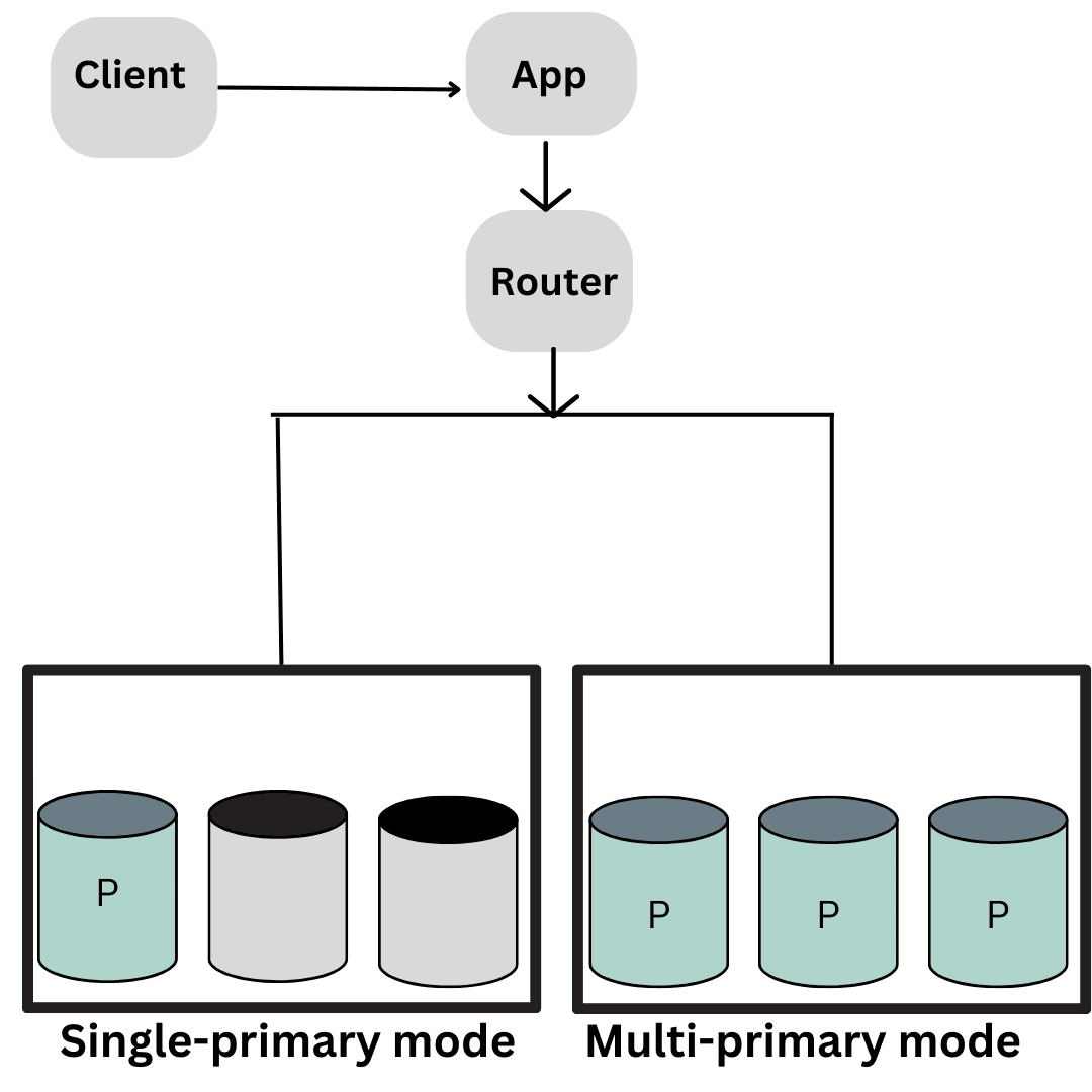
MySQL’s group replication was designed to give a high availability, fault tolerant database cluster. It operates using a multi-master replication approach, allowing multiple MySQL server instances to collaborate as a group, ensuring data consistency and availability. This feature ensures high availability by allowing multiple servers to work together, and if one server fails, another server in the group takes over, minimizing downtime and ensuring continuous access to the data.

Group replication can operate in single-primary mode (default), where only one server (which is the primary server) can accept write operations at a time, or multi-primary mode, where multiple servers can accept write operations simultaneously.


Group replication uses a certification-based replication protocol to ensure that data remains consistent across all servers in the group. In the event of a primary server failure, group replication automatically elects a new primary server to handle write operations, ensuring uninterrupted service by employing middleware devices such as network load balancers or routers. Additionally, it supports both synchronous and asynchronous replication modes, providing flexibility based on your application’s requirements.

Configuring group replication

In order to use MySQL Group Replication, you need to install and configure the plugin on each server in the group. This plugin is designed specifically for the MySQL server and enables you to replicate data across multiple servers, ensuring that your data is always secure and consistent.

By following the installation and configuration instructions carefully, you can ensure that your MySQL group replication setup is both efficient and effective. Here’s a step by step guide to help you demonstrate the process of configuring the group replication:

Ensure that the group replication plugin is installed and activated on each server instance

The MySQL Server 8.0 comes bundled with the Group Replication plugin, so there is no need for extra software. However, it is essential to install the plugin on the active MySQL server to enable its functionality. To install the Group Replication plugin on the active MySQL servers, follow these steps:

i. Check Plugin Availability: First, ensure that the group replication plugin is available in your MySQL installation. Starting from MySQL 8.0, the plugin is included by default, but it’s a good practice to verify its presence. You can do this using the following command:

SHOW PLUGINS;


ii. Connect to MySQL: Use the MySQL client or MySQL Shell to connect to the MySQL server where you want to install the plugin. You need appropriate administrative privileges (e.g., the root user) to perform the installation.

iii. Install the Plugin: Run the following SQL command to install the Group Replication plugin:

INSTALL PLUGIN group_replication SONAME 'group_replication.so';

If you are using Windows, use ‘group_replication.dll’ instead of ‘group_replication.so’.

iv. Verify Installation: To confirm that the installation was successful, you can check the installed plugins by running:

SHOW PLUGINS;

Make sure that ‘group_replication’ appears in the list of installed plugins.

v. Repeat for Other Servers: Repeat the above steps for each of the active MySQL servers that you want to be part of the Group Replication cluster.

It’s important to note that when setting up a Group Replication cluster, all servers should have the same version of MySQL and identical configurations. Also, ensure that you have a backup of your data before making any significant changes to your MySQL installation.

Monitoring group replication 

Monitoring group replication using the performance schema in MySQL involves utilizing a powerful feature that provides the metrics for analyzing the performance of various database activities, including replication. The performance schema allows you to gather detailed insights into how your group replication setup is performing, identify bottlenecks, and diagnose issues. Here’s how you can monitor group replication using the performance schema:

1.Enable Performance Schema: Ensure that the performance schema is enabled in your MySQL server. You can do this by editing the MySQL configuration file (my.cnf or my.ini) and setting the appropriate configuration option, usually “performance_schema=ON”.

2. Relevant Performance Schema Tables: The performance schema provides a range of tables that store information about different aspects of MySQL’s performance, including replication. The key tables related to group replication monitoring include:

i. replication_group_members: This table provides information about the members of your replication group, their status, roles, and more.

ii. replication_connection_status: This table offers details about the connection status between replication group members.

iii. replication_applier_status_by_worker: This table provides information about the status of applier workers on each member, including replication lag and progress.

iv. replication_group_member_stats: This table contains various statistics related to replication for each group member, including transaction counts and sizes.

Running Queries and Analyzing Data

You can run SQL queries against these performance schema tables to retrieve insights into your group replication setup. For example:

To monitor the overall health and state of the replication group, the following query is issued:

SELECT * FROM performance_schema.replication_group_members;

To monitor a group replication members performance, the following query is used:

SELECT * FROM performance_schema.replication_group_member_stats\G

You can also monitor group replication with GTIDs. This is a crucial task which helps to maintain the dependability and consistency of your database. GTIDs (Global Transaction Identifiers) are unique identifiers that are allocated to each transaction in a MySQL database. This makes it simpler to track changes across multiple servers. For more information on GTID, check out part 4 of this series.

To effectively monitor group replication with GTIDs, powerful tools such as MySQL Enterprise Monitor or Percona Monitoring and Management are utilized. These tools allow you to keep an eye on your replication group’s status, assess transaction performance and latency, and diagnose any issues that may arise. It is highly recommended to regularly monitor your replication group to guarantee that it is functioning correctly and to detect potential issues early on. 

Best practices for group replication

To achieve a successful MySQL group replication, it’s crucial to ensure that:

1. All members in the group are using the same version of MySQL

2. All members have identical configuration settings

3. All members are connected through a reliable network

It’s also essential to monitor the group’s status regularly and perform backups to maintain data safety in case of failures. Limiting the number of members in the group can reduce the likelihood of conflicts and ensure efficient replication. Consistency and communication are the main factors in maintaining the group’s success.

Conclusion

MySQL group replication is an important topic in replication. It helps multiple server instances to collaborate as a group. This article is beginner friendly and only highlights the important aspects of using the group replication technique. For more in-depth information, please visit the official MySQL blog and documentation.

The post A Beginners Guide to MySQL Replication Part 5: Group Replication appeared first on Simple Talk.


from Simple Talk https://ift.tt/xOe8CDt
via

Saturday, August 26, 2023

Yet Another Reason to Not Use sp_ in your SQL Server Object Names

In 2012, Aaron Bertrand said most everything I knew (and a bit more) about the issues with using the sp_ prefix. Procedures prefixed with sp_ have special powers when placed in the the master database in that it can be executed anywhere on the server after that. Nothing much has change in those suggestions.

It isn’t that such objects are to be completely avoided, it is that they are ONLY to be used when you need the special qualities. Ola Hallengren’s backup solution creates a dbo.sp_BackupServer procedure so you can run the backup command from any database.

But if you don’t need the special properties of the sp_procedure, they are bad for the reasons Aaron stated, the reason I stumbled upon today being just a special subset. In this case CREATE OR ALTER behaves differently than CREATE in a way that was really confusing to me as I was working on a piece of code today.

My problems are going to be simple code management issues where some code existed in the master database and it confused me as to why something was working, and then why it wasn’t.)

I had accidentally executed the procedure create script in the master database. (I know, I am the only person with this mistake to their name. But if there is no USE statement to start off a script, when I am testing out code it often ends in master. I don’t have access to ANY production resources, so I am usually playing with other people’s code. It is in fact a good reason to change your default database to tempdb.)

Using CREATE OR ALTER

So I executed something like the following:

USE master; --I clearly didn't have a USE 
            --statement in my code!
GO
CREATE OR ALTER PROCEDURE dbo.sp_DoSomethingSimple
AS
 BEGIN
        --format for easier access in writing
        SELECT CAST(DB_NAME() AS VARCHAR(30)) AS DatabaseName;
 END;
GO

Then, later in my testing, I did something like this:

USE WideWorldImporters
GO
EXECUTE  dbo.sp_DoSomethingSimple;
GO

This worked fine and returned:

DatabaseName
------------------------------
WideWorldImporters

Seemed fine. So, I went to drop and recreate this procedure with a new column in the output.

CREATE OR ALTER PROCEDURE dbo.sp_DoSomethingSimple
AS
 BEGIN
     SELECT CAST(DB_NAME() AS VARCHAR(30)) AS DatabaseName,
           CAST(USER_NAME () AS VARCHAR(30)) AS UserName;
 END;
GO

This is where it gets weird, and where your developer is going to be confused… quite confused. It said it did not exist, even though I just executed it:

Msg 208, Level 16, State 6, Procedure sp_DoSomethingSimple, Line 1 [Batch Start Line 34]

Invalid object name 'dbo.sp_DoSomethingSimple'.

Well, I never. I just executed this procedure, and it was there. And EVEN IF IT WEREN’T, I said CREATE OR ALTER. So, create it. A few more rounds like this, a stop for a snack and maybe fight a few Goombas on Mario Brothers, and then a few more rounds against the query compiler… it hit me. I bet I saved this in the master database. So, I cleared it out and all was okay.

But for sake of demonstration, let’s leave that object right where it was. In the master database. This code will make sure that the procedure is only in master, not in your current database:

SELECT  'master', CONCAT(OBJECT_SCHEMA_NAME(object_id),
                '.',OBJECT_NAME(object_id))
FROM    master.sys.procedures
WHERE   name = 'sp_DoSomethingSimple'
UNION 
SELECT  CAST(DB_NAME() AS NVARCHAR(30))
                , CONCAT(OBJECT_SCHEMA_NAME(object_id),
                '.',OBJECT_NAME(object_id))
FROM    sys.procedures
WHERE   name = 'sp_DoSomethingSimple'
GO

/*

This should only return:

------------------------------ ----------------------------
master                         dbo.sp_DoSomethingSimple

If it just has the one row for master, we can continue on.

Ok, so let’s do far more dangerous version of this. Let’s try to drop the procedure. CREATE OR ALTER didn’t change anything, so other than confusing me, not a big deal. But what about:

USE WideWorldImporters
GO
DROP PROCEDURE dbo.sp_DoSomethingSimple;
GO
EXECUTE  dbo.sp_DoSomethingSimple;
GO

Uh oh. I have just silently dropped the master procedure that I really didn’t want to lose.

Msg 2812, Level 16, State 62, Line 77
Could not find stored procedure 'dbo.sp_DoSomethingSimple'.

Of course, I can create the procedure in the WideWorldImporters database now, but it is only available to my database. If that is what you wanted, then that is fine, but if not, you will eventually hear about it. Hopefully you won’t have to admit it was your fault, but if it is, blame the person who used sp_ as the prefix, unless that was you too…

Using CREATE and DROP

Finally, what if instead of CREATE OR ALTER, you had just used CREATE? Assuming you have been following along, there should not be a sp_DoSomethingSimple in either place now, but I added code to make sure:

USE master; 
DROP PROCEDURE IF EXISTS dbo.sp_DoSomethingSimple;
GO
USE WideWorldImporters;
DROP PROCEDURE IF EXISTS dbo.sp_DoSomethingSimple;
GO

After dropping the procedures, try executing the following:

USE master; 
GO
CREATE PROCEDURE dbo.sp_DoSomethingSimple
AS
 BEGIN
        --format for easier access in writing
        SELECT CAST(DB_NAME() AS VARCHAR(30)) AS DatabaseName;
 END;
GO
USE WideWorldImporters
GO
CREATE PROCEDURE dbo.sp_DoSomethingSimple
AS
 BEGIN
        SELECT CAST(DB_NAME() AS VARCHAR(30)) AS DatabaseName,
                   CAST(USER_NAME () AS VARCHAR(30)) AS UserName;
 END;
 GO

If the procedures did not exist, no error occurred. If that wasn’t fun enough to say “no sp_ procedures”, then I have one more reminder:

Use WideWorldImporters;
DROP PROCEDURE dbo.sp_DoSomethingSimple;

Returns the following message:

Commands completed successfully.

Run it again:

DROP PROCEDURE dbo.sp_DoSomethingSimple;/*

Same return message, you just dropped the one in master. But what you thought happened was that the first DROP PROCEDURE failed. Or you probably did, I know that was my first reaction. A third execution will get you the message you expected:

Msg 3701, Level 11, State 5, Line 126

Cannot drop the procedure 'dbo.sp_DoSomethingSimple', because it does not exist or you do not have permission.

Changing the syntax to DROP PROCEDURE IF EXISTS will not change the outcome of the following batches. The second execution will still drop the master copy. If you use the sort of code we used before IF EXISTS existed:

IF EXISTS (SELECT * 
           FROM sys.objects 
           WHERE OBJECT_ID('dbo.sp_DoSomethingSimple') = 
                                                 object_id)
DROP PROCEDURE dbo.sp_DoSomethingSimple;

Then it would not drop the master copy (but to use a cumbersome prefix like sp_, is it worth not being able to say DROP PROCEDURE IF EXISTS?)

Conclusion

Only use sp_ as a prefix to your procedure if you need it, and then it goes in the master database. Otherwise, you may get pretty confused one day when a system object stops working because it doesn’t always work like you expect.


The post Yet Another Reason to Not Use sp_ in your SQL Server Object Names appeared first on Simple Talk.


from Simple Talk https://ift.tt/Wza2xsd
via