Tuesday, March 12, 2019

Help Shape the Future of SQL Monitor

Each year, Redgate runs a survey to ask the folks at companies, from DBAs and Devs to CIOs, about how they monitor SQL Server. Those insights help us understand how we can make SQL Monitor more valuable to DBAs – or anyone responsible for the “care and feeding” of a SQL Server.

The Estate Management features, available with v9, were developed based on feedback from customers like you. Giving you a way to see where you need to spend your time each day and helping you take care of small issues before they become big ones are some of the benefits you’ll see with SQL Monitor.

If you would like a copy of last year’s report, you can find it here. I do hope that you will participate in the 2019 survey which closes on April 5th. It’s a short survey that should take you less than 10 minutes to complete, and you’ll be eligible to win a $250 Amazon Voucher. We would love to hear about the issues you face managing your SQL Server estate, be that one instance or a thousand!

The post Help Shape the Future of SQL Monitor appeared first on Simple Talk.


from Simple Talk https://ift.tt/2EZfrmN
via

Sunday, March 10, 2019

SQLBits and Data in Devon 2019

This is my first blog in a while and I’m sorry it’s not a technical one.  You may be aware but I’m one of the SQLBits organisers which means that for the last few months all my spare time has been devoted to SQLBits organisation.

We were really pleased with how the event went and all the feedback has been really positive.  If you’d like to get involved in helping next year please email us at Helpers@sqlbits.com and we’ll add you to the list.  We can’t guarantee you’ll get to help all days but every new person who volunteers will at least get offered to help on Saturday.

What we should really be doing now is resting after the busy few months we’ve had but because myself and Jonathan (@Fatherjack) are fools we have decided to run our own event in April 2019.  Data in Devon (Formerly known as SQL Saturday Exeter) is running on 26 and 27th April.  This event is part of the Global Azure Bootcamp and is happening at The Jurys Inn, Exeter, Devon.

Friday 26th April has 5 MVPs running deep dive workshops into topics at the bargain price of £175 during March where the price goes up to £200.  The workshops are:

– BI in Azure by Alex Whittles
 Infrastructure as Code with Terraform by John Martin
– Machine Learning: From model to production using the cloud, containers and Dev Ops
– Performance Pain Reduction for Data Platform Projects by William Durkin
– Getting up to speed with PowerShell” by Rob Sewell

The Data in Devon “main event” will be on Saturday 27th of April with 4 parallel tracks and 7 sessions per track, with expert speakers from the UK, Europe and the USA. Attendance for the Saturday is free and includes all of the training sessions and plenty of coffee and other refreshments to keep you going all day.

Take a look at the session schedule and then sign up while tickets are still available!

Hopefully you’ll see something of interest and come and join us in the South West of England.  If not we hope to see you at another event very soon.


The post SQLBits and Data in Devon 2019 appeared first on Simple Talk.


from Simple Talk https://ift.tt/2TtAEzj
via

Friday, March 8, 2019

Discovering Three or Four Part Names in SQL Server Database Code

I am in the middle of a project to enable our corporate databases to work with continuous integration using RedGate SQL Automation (and hopefully get a few blogs/articles out of it too.) One of the things that the tool does is create your database in multiple ways, with multiple names, in order to compare to existing databases and generate a deployment package. The ability to generate your empty database on a server with no other databases is a goal that simplifies this process (and simplifies your test processes as well).

In order to make this work, one of the considerations is to eliminate cross database dependencies, as you can’t reference objects that don’t exist in views, and even in stored procedures, which offer delayed resolution of objects, you can’t test the code without the database it is referencing.

In addition, and somewhat more important to the process, is dealing with three part names that reference the name of the database your object is in. During the comparison process, the database can be created with a name that is different from your target database to compare to (referred to as a shadow database.) So if you are in database X and have references to X.schema.table, but the database is generated as X_Shadow, the X. is now a cross database reference rather than the local reference you are desiring.

Four part names to linked servers are a different sort of nightmare, but one that is (hopefully) exceedingly rare. The queries presented will help with this as well.

Some of our databases have cross database dependencies by design. For example, a staging database may be accessible from loading code in the base database. Or we may have added a bolt on database, like a database of views or user space that we allow cross references to. In all cases however, we need to know what those dependencies are so we can handle them, and ferret out invalid ones.

To illustrate, I will use the following database with a set of references to the WideWorldImporters database.

CREATE DATABASE TestDependencies
GO
USE TestDependencies
GO
CREATE SCHEMA Demo;
GO
--view that accesses WideWorldImporters
CREATE VIEW Demo.WWCities
AS
SELECT Cities.CityID, Cities.CityName
FROM   WideWorldImporters.Application.Cities
GO
--view with local three part name. Bad practice
CREATE VIEW Demo.WWCityCall
AS
SELECT WWCities.CityId, WWCities.CityName
FROM   TestDependencies.Demo.WWCities
GO
--procedure that references a non-existant db
CREATE OR ALTER PROCEDURE Demo.WideWorldI
AS
BEGIN
        SELECT * 
        FROM  WideWorldI.Application.Cities
END
GO
--procedure with dynamic SQL to foreign database
CREATE OR ALTER PROCEDURE Demo.DynamicSQL
AS
BEGIN
        DECLARE @query nvarchar(MAX)
        SET @query = 'SELECT * 
                      FROM WideWorldImporters.Application.Cities'
        EXEC (@query)
END
GO

The following query will give you the cases of three and four part names that are being specifically used in the database. It uses the sys.sql_expression_dependencies view that will give you references to any object from any object, filtered such that the referenced database name isn’t null (if the third part of the name is null, it is a local reference, everything is awesome.)

SELECT OBJECT_SCHEMA_NAME(objects.object_id) 
                            AS referencing_schema_name,
       objects.name AS referencing_object_name,
          objects.type_desc referencing_object_type,
          CASE WHEN referenced_database_name = DB_NAME() 
                  AND referenced_server_name IS NULL 
            THEN 'Internal' ELSE 'External' END 
                        AS referenced_database_location,
COALESCE(sql_expression_dependencies.referenced_server_name,  
         '<localserver>') AS referenced_server_name,
       sql_expression_dependencies.referenced_database_name,
       sql_expression_dependencies.referenced_schema_name,
       sql_expression_dependencies.referenced_entity_name 
                                    AS referenced_object_name
FROM sys.sql_expression_dependencies
                JOIN sys.objects
                        ON objects.object_id = 
                   sql_expression_dependencies.referencing_id
WHERE referenced_database_name IS NOT NULL
ORDER BY referencing_schema_name,referencing_object_name

You can see from the results that due to late binding of names in stored procedure objects, it doesn’t care that the database WideWorldI doesn’t exist. It just shows it as a dependency, just like it did for the real WideWorldImporters reference. A column not returned is the referenced_id column that can tell you if internal database stuff currently exists or not, but it does not capture ids of external objects, those are resolved when you execute the object.

The internal problems are easily fixed, but the external ones can be trouble for trying to build a database from a script. Our solution for generating empty databases with three part names was to designate “families” of databases that we must generate together, so if you are building database X, then you need to build XPrime first and allow cross database only from X to XPrime.

One last note, you can’t be 100% sure that you have everything due to possibility of uncompiled bits of code in dynamic SQL, as I included in one of the example bits of code. A tool you can use for this is sys.dm_db_uncontained_entities, which is meant for checking containment status of the db.

We will be interested in Dynamic SQL references, which will return as an unknown condition, because it is not possible to know what the dynamic SQL will access (and a truly stupid (or evil) programmer can make a string that cannot be searched for like ‘W’ + ‘ideW’ + ‘orldImporters.’ + ‘Application.Cities’. This could not be foun which you could never find with a simple query of the text of your objects.

SELECT OBJECT_SCHEMA_NAME(objects.object_id) 
                            AS referencing_schema_name,
       objects.name AS referencing_object_name,
          objects.type_desc referencing_object_type,
       dm_db_uncontained_entities.statement_type,
       dm_db_uncontained_entities.feature_type_name,
       dm_db_uncontained_entities.feature_name, 
       statement_line_number
FROM   sys.dm_db_uncontained_entities
                 JOIN sys.objects
                        ON dm_db_uncontained_entities.major_id = 
                                             objects.object_id
WHERE  class_desc = 'OBJECT_OR_COLUMN'
  AND  feature_name = 'Dynamic SQL'
ORDER  BY referencing_schema_name,referencing_object_name

For our database, this returns the procedure I built with dynamic SQL, which you should make sure and check:

Note that this query may be quite slow, as it needs to comb through all of your code and check for all sort of issues in containment, and all of your code. The key here is, just how much dynamic SQL you have. If you have a lot of it, this could be a futile effort to hand check all your code. (if possible, I would highly consider you have automated tests of dynamic SQL to check for such abuses)

Assuming your programmers are not monsters, you could also consider SQL Search from Redgate, and search for the name of likely database references. Bonus tip: Dynamic SQL is a pain in many ways, and this is just one additional example.

The post Discovering Three or Four Part Names in SQL Server Database Code appeared first on Simple Talk.


from Simple Talk https://ift.tt/2TmNIWZ
via

Wednesday, March 6, 2019

Introduction to SQL for Cosmos DB

One of the interpretations of the term NoSQL is “Not Only SQL.” Whether this is a factual statement, or an aloof remark is open to debate. However, no one can deny that more and more non-relational data sources are being used in a range of environments. This often leads to both SQL and NoSQL technologies being used side by side despite the differences in both the structures of the data itself and the engines that store the information.

The inevitable challenge for traditional database developers and DBAs is the investment in time and effort required to master a new set of technologies and any new languages required to handle NoSQL data. Fortunately for SQL developers (and indeed for anyone with a decent grounding in SQL) the developers of Cosmos DB have spared a thought for the millions of SQL users who need a path into the brave new world of NoSQL. They have achieved this by providing an SQL API to access JSON-formatted documents stored in Cosmos DB.

This approach brings one instant and overarching advantage for SQL Server (or other relational database) programmers: you are instantly at home with the core language used to extract data.

However, JSON documents are far removed from relational structures and NoSQL document stores are very different beasts compared to relational databases. Consequently, the SQL used to query JSON documents is different in many ways to the conventional SQL that you use with SQL Server. Moreover, Cosmos DB SQL is severely limited compared to T-SQL Yet despite its restrictions, the Cosmos DB SQL API provides an easy path to understanding and exploiting document databases. Acquiring a working knowledge of how to query Cosmos DB could open up new horizons that enable you to integrate data from the relational and NoSQL worlds.

The Basics

Cosmos DB is a multi-model NoSql database. Currently it can handle three types of non-relational data:

  • Document databases
  • Graph databases
  • Key-value databases

Only one of these data models can be queried using SQL in Cosmos DB. This is the document database. Indeed, this is probably a good place to add that Cosmos DB SQL only concerns querying document databases. There is no DDL (data definition language) involved.

A document database is a non-relational database designed to store documents that have no fixed structure. The leading document databases use JavaScript Object Notation (JSON) as the format for structuring the data. The good news with a lightweight and easily modifiable approach like this, is that you are not bound by a rigid schema. The bad news is that you are not bound by any schema at all. This fluidity has many sterling advantages but comes at a cost when querying the JSON data. The two main challenges that you are likely to face as a SQL developer are:

  • Schema on read – Instead of the database schema being part of the database structure, any required structure is defined when the query is written.
  • Nested structures – JSON documents are objects that can contain the complete data describing a self-contained unit. They can be extremely complex and represent a structure that would require a series of tables in a SQL Server database.

Fortunately, Cosmos DB SQL has been adapted to help you overcome the challenges inherent in using a relational database query language to query non-relational data stored in the nested structures of JSON-as you will see in the subsequent article.

When Would you Need Cosmos DB SQL?

Before leaping in to the minutiae of a new or at least a slightly different-dialect of a programming language, you may be forgiven for wondering why you should need to make the effort to master it in the first place. A few potential reasons are:

  • Cosmos DB can store JSON documents at a scale that is truly impressive, and that makes it into an excellent repository when dealing with terabytes of JSON files. SQL Server’s capabilities as a JSON document store are completely overshadowed by Cosmos DB.
  • Cosmos DB can become an ideal complement to SQL Server as a JSON storage service. This is because SQL Server provides analytical capacities that are missing from Cosmos DB. In practice, you can extract finely filtered data from a vast store of documents in Cosmos DB and then load this (infinitely smaller dataset) into SQL Server tables as rowsets for in-depth analysis. This can avoid having to implement a totally different set of technologies to deliver analytics over JSON document stores.
  • You can use PolyBase in SQL Server 2019 to connect to Cosmos DB collections. In this case you will probably need some basic Cosmos DB SQL to flatten the JSON data so that it can be used as an external table.
  • Even if you rely only on Cosmos DB to analyze JSON data you will likely need this Cosmos DB flavor of SQL when writing JavaScript-based stored procedures and user-defined functions.
  • If you are connecting to Cosmos DB using ODBC you are likely to need to flatten the JSON data. This approach will inevitably require the use of Cosmos DB SQL.
  • You can use Cosmos DB SQL SQL API (and SQL over JSON document collections) as the data source in Azure Data Factory activities.

There are, doubtless many other reasons, but I hope that some of these will encourage you to start looking at Cosmos DB.

The Required Toolkit

You need one of two things to practice SQL in Cosmos DB:

  • A Cosmos DB account in Azure
  • The Cosmos DB Emulator which is beautifully explained in this Simple-Talk article.

For the purposes of this article, I will presume that you are using the Cosmos DB Emulator-although either the emulator or Cosmos DB in Azure will work equally well when learning to query JSON documents using SQL.

Sample Data

As this article is a gradual introduction to querying Cosmos DB documents, you will be using simple JSON documents stored in a single collection in Cosmos DB.

The JSON structure that you can use to practice the basics of SQL queries using Cosmos DB is completely flattened, and looks like this:

{
   "CountryName":"United Kingdom",
   "MakeName":"Ferrari",
   "ModelName":"Testarossa",
   "Cost":52000.0000,
   "RepairsCost":2175.0000,
   "PartsCost":1500.0000,
   "TransportInCost":750.0000,
   "Color":"Red",
   "SalePrice":65000.00,
   "LineItemDiscount":2700.00,
   "InvoiceNumber":"GBPGB001",
   "SaleDate":"2015-01-02T08:00:00",
   "CustomerName":"Magic Motors",
   "SalesDetailsID":1
}

Using the Sample Data

The sample documents are in the attached zip (CosmosDBQueries.zip) file which you should install onto your C: drive in the C:\CosmosDB directory. The seven documents that make up the collection are in the simplecars subdirectory.

The first thing to do is to create a collection. I suggest using /CountryName as the partition key in this example. As creating databases and partitions is explained in the article referenced above, I will not go through it again it again here. Then you need to load the documents. As there are only a handful of them, you can just click the New Document button and paste the contents of each file into a separate document, and then save it.

There is also the Upload option for loading multiple files which you can use instead. However, this does not seem to work at the moment in the Cosmos DB Emulator.

Of course, in the real world, there are solutions that you will need to learn if you are loading hundreds of thousands of documents and terabytes of data. However, these techniques are out of scope for this simple introduction.

Basic Terminology

For the sake of clarity, there are a few basic definitions that should help you bridge the gap between SQL and the world of JSON documents:

  • A collection can be considered to be a database
  • A document equates broadly to a recordset (although the nested structure makes it more similar to XML)
  • An attribute is a field or column

These points of comparison are not destined to be taken too literally and are simply provided as an initial stepping stone to help with your initial understanding if you have never seen document databases before.

Basic SQL Queries

Begin with the simplest possible example. With the Cosmos DB Emulator running, enter and execute the following query:

SELECT * FROM C

You will see all the documents in the current collection returned as the output, each one similar to the sample document shown above.

As simple as this query may be, as it is the first query that you have created with Cosmos DB SQL a few comments are in order. Firstly, the data is returned as JSON, even if you are using SQL to query the documents. In effect, JSON is the data format. A second point is that you cannot specify the collection to query in the SQL. Consequently, you need to ensure that you open a query window from the required collection. However, you can use anything as the definition of the data source. The query could read:

SELECT * FROM thecurrentcollectionbecauseIlikedreamingaboutcars

When running simple queries, the source JSON is returned as it exists in the collection. You will learn how to shape the output JSON later in this article and in the second article in this series.

A final point to note is that, technically, you can also return a complete JSON document with this SQL:

SELECT * FROM ROOT

Now to be a little more selective, try this short query:

SELECT   saleselements.InvoiceNumber
        ,saleselements.TotalSalePrice
FROM    saleselements

This is the output you should see the following (here, obviously, is a truncated view of the output):

{
        "InvoiceNumber": "GBPGB001",
        "TotalSalePrice": 65000
    },
    {
        "InvoiceNumber": "GBPGB011",
        "TotalSalePrice": 89000
    }

Executing this query only returns two of the available JSON attributes. What is worth noting here is that you must use the collection name or alias when referencing attributes. It is generally easier to use short aliases for the collection, like this:

SELECT s.InvoiceNumber, s.TotalSalePrice  
FROM saleselements AS s

The AS keyword when aliasing collections is optional. Attribute names are case-sensitive, although misspelling them will not stop the query executing it will prevent the attribute from being returned in the output.

Of course, you can add aliases to attributes:

SELECT s.InvoiceNumber, s.SalePrice AS Price
FROM   saleselements AS s

Doing this will deliver the following JSON:

{
        "InvoiceNumber": "GBPGB011",
        "Price": 8500
    }

However, when aliasing attributes you need to remember that:

  • The AS keyword is optional
  • Aliases are case-sensitive.
  • Aliases must respect JavaScript naming conventions – you cannot start an alias with a number or other non-alphabetical character except the dollar sign or underscore

You cannot add an alias to * so you cannot write

SELECT c.* FROM c

I realize that the JSON specification calls attributes “members” and the data for each member an element, yet the use of the word attribute to describe the name of a piece of data is so prevalent I prefer to use it.

Cosmos DB SQL will return strings, numbers and dates exactly as they are stored in the JSON document – as you can see if you try this query:

SELECT   s.InvoiceNumber
         ,s.SaleDate
         ,s.SalePrice
FROM     saleselements AS s

The result will be:

{
        "InvoiceNumber": "GBPGB011",
        "SaleDate": "2015-04-30T00:00:00",
        "SalePrice": 8500
}

Of course, Cosmos DB SQL can perform basic arithmetic:

SELECT   s.InvoiceNumber
         ,s.SalePrice - s.Cost AS GrossProfit
FROM     saleselements AS s

As you can see below:

{
        "InvoiceNumber": "GBPGB011",
        "GrossProfit": 1700
}

As a variation on a theme, you can always write SELECT clauses like this:

SELECT   s["InvoiceNumber"]
         ,s["SaleDate"]
FROM     saleselements AS s

Indeed, you can mix and match the ‘alias dot attribute’ notation and the ‘alias square bracket and double quote’ notation (in which case there are no dots used to link the alias and the attribute name) inside the same query.

Simple WHERE Clauses

Time to move on to data selection. After all, Cosmos DB can store terabytes of JSON documents and allows you to scale queries to use more or less processing power so that you can balance the requirements of query time and cost (in the financial sense) to suit each individual requirement.

A Basic Text Filter

Suppose that you want to isolate all invoices where a Bentley was sold. This should not tax your SQL knowledge, and hopefully will reassure you that Cosmos DB SQL cleaves to basic SQL tenets:

SELECT   s.InvoiceNumber ,s.SalePrice
FROM     s
WHERE    s.MakeName = "Bentley"

You should see a result like the following:

{
        "InvoiceNumber": "GBPGB011",
        "SalePrice": 80500
}

Yes, you are using double quotes to enclose a string. This may come as a surprise to SQL Server developers (although possibly less so to users of other databases). To be fair, you can also use single quotes if you feel that you are otherwise betraying your SQL heritage.

Numeric Filters

Filtering on numbers in JSON attributes is probably what you would expect it to be. You could write a WHERE clause like this one to specify a precise figure:

SELECT   s.InvoiceNumber ,s.SalePrice
FROM     s
WHERE    s.LineitemNumber = 2

Or like this one to define a numeric range:

SELECT   s.InvoiceNumber ,s.SalePrice
FROM     s
WHERE    s.Cost BETWEEN 50000 AND 100000

Here, the result will be:

{
        "InvoiceNumber": "GBPGB011",
        "SalePrice": 8500
}

And now is the disconcerting part. You can filter on a field and include it in the SELECT clause at the same time-like this (although this will indicate the filter validity in the results):

SELECT   s.InvoiceNumber, s.Cost BETWEEN 50000 AND 100000 
           AS InCostRange, s.SalePrice
FROM     s

This query will give the following result:

{
        "InvoiceNumber": "GBPGB011",
        "InCostRange": false,
        "SalePrice": 8500
}

To conclude the subject of elementary WHERE clauses, you can also reassure yourself that:

  • The AND, OR, NOT operators function pretty much as they do in T-SQL
  • =, !=, >=, <=, <> operators allow you to specify threshold values in queries
  • You can use parentheses to create more complex query logic

Alphabetical Ranges

If you ever need to return documents based on an alphabetical range in an attribute, then one way of obtaining the desired result is to use this kind of SQL:

SELECT   s.CustomerName ,s.SalePrice
FROM     saleselements AS s
WHERE    SUBSTRING(s.CustomerName, 0, 1) BETWEEN "A" AND "M"

Date and Time Filters

Cosmos DB SQL does allow for some more advanced filtering methods in the WHERE clause. Although the possibilities are, it has to be said, considerably more limited than those offered by T-SQL, you can, nonetheless, include (and exclude) irrelevant JSON documents by filtering on date and time elements.

JSON does not have a date type, as such. Instead it uses a string. Consequently, you risk encountering dates in any of a myriad of formats. The upshot is that you will be delving into the specific string format to filter on dates and times.

The format in the sample data is in something close to the ISO 8601 format, which looks like this: YYYY-MM-DDTHH:MM:SS. This means that searching for a specific date and time means representing the datetime as an ISO string, in this way:

SELECT s.SaleDate
FROM   s
WHERE  s.SaleDate = "2015-01-02T08:00:00"

If you are looking to set an upper or lower boundary for a date or time you can use the standard comparison operators: >=, <=, <> or !=.

Using Date Ranges

It follows that defining a date range requires nothing more than a simple AND operator in the WHERE clause.

SELECT s.SaleDate
FROM   s
WHERE  s.SaleDate >= "2015-01-01T00:00:00"
       AND
       s.SaleDate <= "2015-01-31T23:59:59"

This returns data from three documents:

[
    {
        "SaleDate": "2015-01-02T08:00:00"
    },
    {
        "SaleDate": "2015-01-25T00:00:00"
    },
    {
        "SaleDate": "2015-01-02T10:33:00"
    }
]

Or, possibly more elegantly, you can use the standard BETWEENAND construction:

SELECT s.SaleDate
FROM   s
WHERE  s.SaleDate BETWEEN "2015-01-01T00:00:00" 
       AND "2015-01-31T23:59:59"

This returns data from the same three documents:

[
    {
        "SaleDate": "2015-01-02T08:00:00"
    },
    {
        "SaleDate": "2015-01-25T00:00:00"
    },
    {
        "SaleDate": "2015-01-02T10:33:00"
    }
]

Applying Time Filters

Filtering by time essentially means extracting the hour, minute and possibly second or millisecond elements from the date string. So, to find all cars sold between 8:45AM and 12AM you would write:

SELECT s.SaleDate
FROM   s
WHERE  SUBSTRING(s.SaleDate, 11, 2) BETWEEN "08:45" AND "12:00"

This should return data from two documents in the collection:

[
    {
        "SaleDate": "2015-02-03T10:00:00"
    },
    {
        "SaleDate": "2015-01-02T10:33:00"
    }
]

The lack of a schema in the JSON documents means that the date could be specified in a completely different string format, or even as a number (say in the YYYYMMDD format where the data shown above would be 20150131).

Clearly the requisite queries would have to be adapted to the date format used, in which case a theoretical query on a totally different collection (where the dates were stored differently) could read:

SELECT s.SaleDate
FROM   s
WHERE  s.SaleDate BETWEEN 20150101 AND 20150131

Yet again the ‘free-form’ nature of JSON means that you will have to display both ingenuity and mental agility in the queries that you write.

Traps for the Unwary

Cosmos DB SQL requires you to wrap non-standard attribute identifiers in double quotes (and square brackets). As I mentioned above, no dot notation is used for the collection alias in this case. If you want to output one of the collection’s built-in attributes, you need to write SQL like this:

SELECT s.InvoiceNumber ,s.SalePrice, s["_rid"]
FROM   saleselements AS s

It is also worth noting that you cannot use unauthorized elements such as leading numbers in aliases even when you enclose the alias in double quotes.

When filtering on texts that contain special characters you need to know that certain characters are escaped in Cosmos DB SQL. Consequently, this is what you need to enter to include these characters in a WHERE clause:

  • Single quote: \’
  • Double Quote: \”
  • Backslash: \\

There are, of course, many others, but I will let you delve into the documentation to find them.

Now that the basics have been covered (and hopefully you are reassured that your SQL skills can be applied to document databases) it is time to look at some aspects of Cosmos DB SQL in greater depth.

Sorting Output

Cosmos DB SQL also contains the ORDER BY clause, so you can write queries like this one:

SELECT   s.InvoiceNumber ,s.SalePrice AS Price
FROM     saleselements AS s
ORDER BY s.InvoiceNumber

It probably comes as no surprise that you will see a result set something like the following:

{
        "InvoiceNumber": "EURDE004",
        "Price": 11500
    },
    {
        "InvoiceNumber": "EURFR005",
        "Price": 19950
    },
    {
        "InvoiceNumber": "GBPGB001",
        "Price": 65000
    },
    {
        "InvoiceNumber": "GBPGB002",
        "Price": 220000
}

However, at this juncture a series of limitations appear on the horizon. For, although you can add the ASC / DESC keywords to an ORDER BY clause (as you can in T-SQL) the following restrictions apply here:

  • The ASCENDING and DESCENDING keywords are not supported
  • Sorting on multiple attributes is not possible
  • You cannot sort on an alias for an attribute – you must reference the attribute preceded by the collection alias and a dot as you do in the SELECT clause
  • You cannot order by anything other than a field name
  • You cannot sort by a computed value

Summarizing Results

Here are several examples for common aggregates:

Finding the Number of Documents in a Collection

The query to return the number of documents in a collection is a slight extension of standard SQL:

SELECT VALUE COUNT(1)
FROM         s

Here you are adding the VALUE keyword to return a number only and not a JSON structure. Consequently, the result looks like this:

[    7
]

You could also write this query as:

SELECT VALUE COUNT(s.id)
FROM s

Very Basic Aggregations

If you want to aggregate data from a collection, you could try a query like this one:

SELECT VALUE SUM(s.SalePrice)
FROM         saleselements AS s

The output is extremely simple:

[
    424950
]

However, some fairly profound restrictions appear here (at least with the current version of Cosmos DB).

  • There can only be one aggregation per query
  • No alias can be added to the aggregation if you are using the VALUE keyword
  • You will get an error if the query is a cross-partition query, and you do not use the VALUE keyword. Cosmos DB partitions (as you might expect) are a core storage and query acceleration design approach. However, creating partitions is a subject in its own right that I cannot go into here

Intriguingly, you can get around the forced use of the VALUE keyword when querying across partitions with the use of a subquery like this:

SELECT * FROM
(SELECT  SUM(s.SalePrice) FROM s)

In this case, the output looks something like this:

[
    {
        "$1": 424950
    },
    {
        "$1": 0
    }
]

You are probably wondering where the $1 attribute names come from. This is, quite simply, what happens when you do not use an alias for a subquery or a function in Cosmos DB SQL. Think of it as being similar to non-aliased columns in T-SQL appearing as (no column name) in the query output.

Using a subquery also allows you to use multiple aggregate values in a calculation. In the following example you can see the difference between the maximum and average sale prices:

SELECT * FROM
(SELECT VALUE MAX(s.SalePrice) - AVG(s.SalePrice) 
FROM s)

As you can see, you do not necessarily have to alias the subquery:

[
    159292.85714285716
]

Of course, you can filter the data set that the calculation is applied to:

SELECT * FROM
(SELECT VALUE MAX(s.SalePrice) - AVG(s.SalePrice) 
FROM s WHERE s.MakeName = "Ferrari")

This gives the corresponding output:

[
    77500
]

As you can see here, applying the VALUE keyword returns just that-a value-and consequently there is no attribute name in the output.

Shaping Output

Cosmos DB SQL allows you to shape the output of an SQL query in several ways – pretty much as ‘ordinary’ SQL does. Some of the techniques that you can apply are described in this section.

Returning the Top N Documents

Cosmos DB SQL imitates T-SQL when it comes to returning only a specified number of documents from a collection. This one does not even need me to show you the result of the query.

SELECT   TOP 3 s.InvoiceNumber, s.SalePrice
FROM     s
ORDER BY s.SalePrice DESC

Concatenate Attributes

The Cosmos DB SQL CONCAT() function is simple yet powerful. Take a look at the following example:

SELECT   CONCAT(s.CustomerName
               ," Date of Sale: "
               ,s.SaleDate) AS CustomerName
FROM     s

This function allows you to join multiple fields and/or static values to produce a single output attribute-like this:

{
 "CustomerName": "Wonderland Wheels Date of Sale: 2015-04-30T00:00:00"
    },
{
 "CustomerName": "Wonderland Wheels Date of Sale: 2015-04-30T00:00:00"
    }

Replacing Values in the Output

Should you need to replace specific values in the resulting JSON, you can use the REPLACE() function. And, yes you can use multiple nested replace operations if you need to.

SELECT   REPLACE(
                 REPLACE(s.CountryName, "United Kingdom", "Blighty")
                 ,"France", "Hexagone") AS Country
FROM     s

Here is the corresponding query output (from the final objects returned by the query):

{
        "Country": "Blighty"
    },
    {
        "Country": "Germany"
    },
    {
        "Country": "Hexagone"
    }

String Functions – Simple Classics

Cosmos DB SQL has most of the basic string functions that you could require. Some of these are used in the following query:

SELECT   UPPER(s.CustomerName) AS CustomerName
        ,LOWER(s.CountryName) AS CountryName
        ,TRIM(s.CountryISO3) AS CountryISO3
        ,LEFT(s.MakeName, 3) AS MakeAbb
        ,RIGHT(s.InvoiceNumber, 3) AS InvoiceNumber
        ,SUBSTRING(s.InvoiceNumber, 3, 2) AS SaleCountry
FROM    s

Here is the result for a single document:

{
        "CustomerName": "WONDERLAND WHEELS",
        "CountryName": "united kingdom",
        "CountryISO3": "GBR",
        "MakeAbb": "Por",
        "InvoiceNumber": "011",
        "SaleCountry": "GB"
}

You need to be aware that:

  • SUBSTRING() is 0 based.
  • You can also use the LTRIM() and RTRIM() functions if you need to.

A Final Few String Functions

Cosmos DB SQL only has a couple of dozen string functions, and we have seen many of the most useful ones already. Should you need them, you can always add the following to your armoury:

REPLICATE()

LENGTH()

INDEX_OF()

Mathematical Functions

Cosmos DB SQL comes complete with a core set of mathematical functions.

SELECT   ROUND(s.TotalSalePrice) AS RoundedSalePrice
        ,FLOOR(s.RepairsCost) AS RepairsCost
        ,CEILING(s.PartsCost) AS PartsCost
        ,TRUNC(s.TransportInCost) AS TransportInCost
FROM    s

Take a quick look at the result:

{
        "RoundedSalePrice": 89000,
        "RepairsCost": 250,
        "PartsCost": 225,
        "TransportInCost": 150
    }

These are considerably more limited than their T-SQL equivalents, and only carry out basic rounding.

There are a few others such as ABS(), SQRT(), SQUARE() plus a small set of trigonometric functions should you need them.

Logic (Imitation CASE Statements) – Ternary Functions

ANSI SQL has the CASE statement. Cosmos DB SQL instead uses a ternary logic approach. That is, it uses the ? and : constants to break up the code into test ? true : false elements.

To see this in action, take a look at the following Cosmos DB SQL snippet:

SELECT s.CountryName IN ("France", "Germany", "Spain") 
                        ? "EU" : "Other" AS Region
FROM   s

This code tests for any of France, Germany or Spain in the CountryName attribute and returns EU if any of these elements are found-and Other if they are not found, as you can see, below:

[
    {
        "Region": "Other"
    },
    {
        "Region": "Other"
    },
    {
        "Region": "Other"
    },
    {
        "Region": "Other"
    },
    {
        "Region": "Other"
    },
    {
        "Region": "EU"
    },
    {
        "Region": "EU"
    }
]

Fortunately Cosmos DB SQL lets you nest ternary logic (as you may have done using the IF() function in Excel or the T-SQL IIF() functions).

SELECT   s.CountryName IN ("France", "Germany", "Spain") 
                       ? "EU" 
                       : s.CountryName = "United Kingdom" 
                            ? "Blighty"
                            : "Other" 
         AS Region
FROM     s

Conclusion

Now that you have a grasp of the basics of Cosmos DB SQL, I hope that you will be tempted to consider using this powerful and scalable document database as a potentially game-changing extension to your relational database environment-and this particular approach to NoSQL as a valuable part of your skillset.

I am not denying that the SQL that is implemented on top of Cosmos DB is severely limited. Although you can often find workarounds to obviate the worst of its restrictions, you are essentially stuck with simple SQL queries that use SELECT, FROM. WHERE and ORDER BY. You will not find any GROUP BY or HAVING clause for instance, and queries are bound to a single collection. Its analytical capabilities are curtailed by the absence of windowing functions.

On the other hand, the sheer simplicity of the query language, as well as the ease with which you can adapt your current skills and learn to query JSON documents without having to learn a new framework and syntax are powerful points in its favour.

However, we have not finished with the guided tour of Cosmos DB SQL yet. A second article will explain some of the more advanced features of the language that can be used to cope with the more complex document structures that JSON allows. This article will also provide some hints and tips on working around some of the limitations inherent in querying JSON documents with SQL.

The post Introduction to SQL for Cosmos DB appeared first on Simple Talk.


from Simple Talk https://ift.tt/2UvBM1u
via

Tuesday, March 5, 2019

Resumable Online Index Create and Rebuild Operations

Did you know that SQL Server supports pausing and resuming the index creation and rebuild processes? The resumable online index rebuild option is currently supported in Azure SQL Database and SQL Server 2017 With the introduction of the public preview of Azure SQL Database and the community technical preview (CTP) of SQL Server 2019, the SQL Server team has enhanced the pause and resume functionality by added the resumable online index create option.

If you have ever had to cancel an online rebuild or create index process on a very large table because the index rebuild or creation process didn’t complete during your maintenance window, or consumed valuable resources causing other queries to run slow, then you need to check out the resumable online index options.

The worse part about canceling the rebuild or index creation process in an older release of SQL Server was that the whole process rolled back, and all that work done prior to the canceling was wasted. It would be nice if you could restart your cancelled online rebuild or create index statement where it left off, instead of starting the index rebuild or creation process all over again.

If you are running SQL Server 2017, you can pause and restart the index rebuild operation, but not the create index options. Although, if your database is running in the preview of an Azure SQL database or SQL Server 2019, you can pause and restart both the online rebuild and index create processes. In this article, I will show you to pause and restart your online index operations.

Overview of Resumable Online Index Operations

When you cancel an index rebuild or a create index operation in SQL Server prior to SQL Server 2017, the database engine must roll back all the work it had done on the index. Because of this, when you restart the index rebuild or create index process, SQL Server has to start all over again at rebuilding or creating the index. This causes lots of processing and requires resources just to redo what was done prior to cancelling the indexing rebuild or create index process.

But if you migrate your older versions of your databases to SQL Server 2017, you can restart your online index rebuild operations. Plus, with the rollout of the previews of Azure SQL Database or SQL Server 2019, you can pause and restart both your online rebuilds and creation processes.

Being able to pause these online index operations allows SQL Server to pick up the rebuild or create index operations where they left off. The ability to retain the work done when pausing an online index operation allows you to perform the index operation in a piecemeal approach. Restarting a create or rebuild an index on a really big table by pausing and resuming the indexing process allows you to work around your short maintenance windows and other resource intensive queries.

Sample Test Data

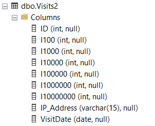
In order to test out the new pause and resume functionality of online resumable index operations, I decided to create a table that contains 60 million rows. If you want to follow along and run the code in this article, you can use the code found in the Listing 7 in the last section of this article titled “Create Sample Data.” (Another option is to create the table and populate it using Redgate’s SQL Data Generator.) That code creates a database named SampleData and then creates and populates the Visits2 table. The table definition looks like the image found in Figure 1:

Figure 1: Definition for table Visits2

I created this database on the CTP 2.2 version of SQL Server 2019, so I could test pausing and restarting both the index creation and rebuild operations. You can download that version of SQL Server here.

How to Pause and Resume an Online Index Operations

To test out the new pause and resume functionality of an online index operation, you will first create a non-clustered index online. The index will be on the I100 column of the Visits2 table using the script in Listing 1. Keep in mind the resumable option for the create index operation is only available in the preview versions of Azure SQL Database and SQL Server 2019 at the time this article was written. You cannot create a resumable online index in any version of SQL Server except the CTP versions I just mentioned.

Listing 1: Create an Online Resumable Non-Clustered Index

CREATE INDEX NC_Visits2_1 ON dbo.Visits2  (I100)
WITH (ONLINE = ON,RESUMABLE = ON);

The RESUMABLE=ON parameter in the WITH clause is what makes this CREATE INDEX command resumable. Note that you also have to include the ONLINE = ON clause when you use the RESUMABLE option. If you leave off the ONLINE option, you will get an error.

The next step of testing out the resumable index creation is to pause the create index process. After allowing the resumable index creation operations to process for a while, you can PAUSE this index create operation, by running the code in Listing 2 in a new query window:

Listing 2: Pausing the resumable online index creation process

ALTER INDEX NC_Visits2_1 ON dbo.Visits2 PAUSE;

When you run the code in Listing 2, you will find that the session that was running the CREATE INDEX statement gets disconnected and the messages in Figure 2 are displayed.

Figure 2: Message from pausing the resumable index creation process

Once you have paused your online resumable index operation you can determine how far along the process progressed prior to being paused by using a new system view that came out in the current version of Azure SQL Database, or SQL Server 2017 named sys.index_resumable_operations. By running the code in Listing 3, you can see how far along the online resumable index creation operation progressed prior to being paused.

Listing 3: Show how far the resumable index create operation got prior to being paused

USE SampleData;
GO
SELECT 
name as index_name,
percent_complete, 
state_desc, 
start_time,
last_pause_time, 
total_execution_time AS ExecutionMin,
-- execution time times 
-- ratio of percent to complete and precent completed
total_execution_time * (100.0-percent_complete)/percent_complete  
    AS ApproxExecutionMinLeft 
FROM sys.index_resumable_operations;

When you run the code in Listing 2, you will see something like the output in Figure 3.

Figure 3: How far the index creation process got prior to being paused

By looking at the pecent_complete column in Figure 3, you can see that the progress shows 64.33% through the creation process. Plus if you look at the state_desc column, in Figure 3, you can see the index creation process is in a PAUSED state. Note you might also want to use the sys.index_resumable_operations system view to review the progress status of your index prior to pausing it, just to see if it is almost finished. No sense in pausing something that is just about ready to complete.

To restart a paused indexing process, all you have to do is run the code in Listing 4 in a query window.

Listing 4: Code to resume the indexing creation process

USE SampleData;
GO
ALTER INDEX NC_Visits2_1 ON dbo.Visits2 RESUME;
GO

When you run the code in Listing 4, the index creation process will pick up where it left off and continue creating the index. You can verify that the index creation process is running again and starts where it left off by running the code in Listing 3 again. The output you get from the second run of this code will show that your index creation process is now running, and the percent completed should be slightly further along than what was shown the first time you ran this code.

When you restart the index process using the code in Listing 4, the ALTER INDEX statement continues to run until the index process completes. When the index is done being created you will get a message indicated that the ALTER INDEX statement completed successfully in the message window.

The next test is to determine if you can run two online resumable index operations on the same table, at the same time. To test that out you can run the code in Listing 5, while the original online resumable index process is running using the code in Listing 1.

Listing 5: Starting a second resumable index operation on same table

USE SampleData
GO
CREATE  INDEX NC_Visits2_2 ON dbo.Visits2  (I100)
WITH (ONLINE = ON,RESUMABLE = ON);

You might be thinking you could start a second non-clustered online resumable online index process on the same table while an existing online reusable index is running. However, if you try to start a second non-clustered online resumable index operation, or any index operation, on the same table as one already running you will get the error showing in Figure 4.

Figure 4: Error when trying to run second resumable online index operation

As you can see you can’t run a second resumable index operation while the first one is running.

You also might think you could just pause the first index operation so you can start the second one. But if you try this you will get the messages shown in Figure 5.

Figure 5: Error message when starting second index operation when another one is paused

As you can see SQL Server does not support running a second online resumable index operations at the same time, even if one of them is paused.

So far, you have just tested out pausing and resuming an online resumable index create operations. But you can also pause and resume an index rebuild operation by adding the RESUMABLE = ON option to your ALTER INDEX statements. The code in Listing 6 shows how you would run an online resumable REBUILD operation on the NC_Visits2_1 non-clustered index.

Listing 6: Code to start an online resumable index rebuild

ALTER INDEX NC_Visits2_1 ON dbo.Visits2 REBUILD 
WITH (ONLINE = ON, RESUMABLE = ON);

As already stated, if you are only running the current GA version of SQL Server, whether it is Azure SQL Database, or SQL Server 2017 you can only perform online resumable index rebuild operations and not index create operations. You need to be running the new CTP version of SQL Server in order to run the online resumable index creation operations.

I think you will agree that being able to pause and restart the online index creation or rebuild processes is a great enhancement, especially when you what to create an index or rebuild and index on a very large table. With this new resumable option, SQL Server makes it simple to pause and restart the online index creation and rebuild processes. Being able to do this provides the ability to better manage resources and maintenance windows while you run a long running online index create or rebuild operation.

Observations

When I was reviewing this new pause and resume functionality for the online index creation and rebuild operations, I made the following observations:

  • You can only pause the index creation process if you have specified the RESUMABLE option on the create or rebuild index statement. If you already have scripts to create or rebuild your indexes online don’t forget to put this new option in your scripts if you want to pause and resume your indexes. Also note you can only use the RESUMABLE=ON option if you also include the ONLINE=ON option as well.
  • When you pause your resumable create index or rebuild operation, the session running the index create or rebuild statement will be canceled and disconnected. The messages you get when this happens seem is a little different than I would have expected (see Figure 2). It would be nice if the messages would have said something like Your reusable index operation has been PAUSED. To restart use the ALTER INDEX with the RESUME option. Since the message about being disconnected is the message that was used to support the online resumable rebuild operation in the current Azure SQL database, or SQL Server 2017, I don’t think the SQL Server team are going to change this message to have any text that references the resumable operation.
  • You cannot cancel your resumable index create or rebuild operation by just terminating these index operations. When you kill or cancel your resumable index operations the index goes into a PAUSED state. To truly cancel your resumable index operation completely you will need run an ALTER INDEX statement with the ABORT option.
  • You can only create one resumable online index operation on a table at a time. It really is too bad you can’t start multiple index rebuild operations if you have the system resources to do it, but this is just the way it works.
  • When using the RESUMABLE option you can also add a MAX_DURATION option. By using the MAX_DURATION, you can set the number of minutes a resumable index create or rebuild operation will run. When that time limit is reached, the resumable index process will be killed, in affect pausing the index creation or rebuild operation. This would be a useful option to use when you want to perform your index operation in a piecemeal approach.
  • When creating a new index using the RESUMABLE option, you will not see it listed in sys.indexes or in SSMS until the operation has completed. To find the index, use the sys.index_resumable_operations system view.

Pausing/Restarting Online Index Operations

The introduction of the resumable online index rebuild feature of SQL Server 2017 and Azure SQL Database, and the addition of the resumable online index create feature that is available in the preview versions of Azure SQL Database and SQL Server 2019 are great improvement to the index create and rebuild function. By having this new pause/restart functionality, you no longer need to run your create index, and rebuild operations as a single uninterrupted process. Being able to pause and resume your online index create and rebuild operations allows you a way to do these operations in a piecemeal approach. If this roll back feature of canceling a rebuild or create online index process has been a pain point, then you should be excited to realize that SQL Server now supports resumable index operations. By moving your database to SQL Server 2017 today, you can get the online resumable index rebuild functionality now. But you are going to have to wait until Microsoft rolls out the newest versions of SQL Server code base into the GA version of Azure SQL Database and SQL Server 2019 in order to use the resumable online index create functionality.

Create Sample Data

In Listing 5, you will find the code I used to create my contrived sample database (SampleData) and the table (Visits2) I used to support my testing for this article.

Listing 7: Create Sample Data

-- Create Sample DB with SIMPLE recovery
CREATE DATABASE SampleData
 CONTAINMENT = NONE
 ON  PRIMARY 
( NAME = N'SampleData', FILENAME = 
         N'D:\SQL Server 2019\SampleData.mdf' 
         , SIZE = 4GB, FILEGROWTH = 1GB)
 LOG ON 
( NAME = N'SampleData_log', FILENAME = 
          N'D:\SQL Server 2019\SampleData_log.ldf' , 
          SIZE = 1GB, FILEGROWTH = 1GB);
GO
ALTER DATABASE SampleData SET RECOVERY SIMPLE;
GO
-- Set database context
USE SampleData;
GO
-- Create table to hold sample data
CREATE TABLE Visits2
(
        ID         INT, 
        I100       INT, 
        I1000      INT, 
        I10000     INT, 
        I100000    INT,
        I1000000   INT, 
        I10000000  INT,
        IP_Address VARCHAR(15),
        VisitDate  DATE
);
GO
-- Create Tally Table
GO
CREATE VIEW vw_Tally AS 
   --Itzik style tally table
   WITH lv0 AS (SELECT 0 g UNION ALL SELECT 0)
     ,lv1 AS (SELECT 0 g FROM lv0 a CROSS JOIN lv0 b) -- 4
     ,lv2 AS (SELECT 0 g FROM lv1 a CROSS JOIN lv1 b) -- 16
     ,lv3 AS (SELECT 0 g FROM lv2 a CROSS JOIN lv2 b) -- 256
     ,lv4 AS (SELECT 0 g FROM lv3 a CROSS JOIN lv3 b) -- 65,536
     ,lv5 AS (SELECT 0 g FROM lv4 a CROSS JOIN lv4 b) -- 4,294,967,296
     ,Tally (n) AS 
        (SELECT ROW_NUMBER() OVER (ORDER BY (SELECT NULL)) FROM lv5)
   SELECT TOP (1000000) n
   FROM Tally
   ORDER BY n;
        
GO      
-- Populate Visits2 with sample data
SET NOCOUNT ON;
DECLARE @Max bigint = (select ISNULL(max(ID),0) From Visits2);
WHILE @Max < 60000000 BEGIN 
        
   WITH TallyTable AS (
        
   SELECT n + @Max as N, 
      CAST(RAND(CHECKSUM(NEWID())) * 255 as INT) + 1 AS A4,
      CAST(RAND(CHECKSUM(NEWID())) * 255 as INT) + 1 AS A3,
      CAST(RAND(CHECKSUM(NEWID())) * 255 as INT) + 1 AS A2, 
         1.0 + floor(1 * RAND(convert(varbinary, newid()))) AS A1,
      DATEADD(DD, 1.0 + floor(62 * 
        RAND(convert(varbinary, newid()))),'2018-07-01') AS VisitDate
                FROM vw_Tally)
        INSERT INTO Visits2 (ID, I100, I1000, I10000,   I100000,
        I1000000, I10000000, IP_Address, VisitDate)
        SELECT  n,n%100, n%1000, n%10000,n%100000,
           n%1000000, n%10000000, 
          CAST(A1 AS VARCHAR) + '.' + CAST(A2 AS VARCHAR) + 
             '.' +  CAST(A3 AS VARCHAR) + 
             '.' +  CAST(A4 AS VARCHAR), VisitDate
        FROM TallyTable 
        set @Max = (select ISNULL(max(ID),0) From Visits2);
END


The post Resumable Online Index Create and Rebuild Operations appeared first on Simple Talk.


from Simple Talk https://ift.tt/2TfWENQ
via

Monday, March 4, 2019

Celebrating Women in Tech

NASA recently named a facility in honour of Katherine Johnson, the mathematician who performed the calculations for space flights in the 50s and 60s. She was one of the “human computers” whose stories were made famous by the movie Hidden Figures just a few years ago. Until that movie was released, the contributions of these women were not well known. Imagine making those calculations by hand today!

There are many women pioneers in technology whose accomplishments outshine anything most of us could do these days. Ada Lovelace wrote the first computer program for a theoretical machine about 100 years before the first real computer existed. Admiral Grace Hopper developed one of the first compilers. The inventions of Hedy Lamarr during World War II lead to the Wi-Fi technologies we all now use.

At the dawn of the computing age, women coders were the norm. Most of the programmers on the ENIAC system were women, for example. Programming was considered low-prestige, unglamorous, and tedious work most suited for women, but even then, women didn’t get credit for their achievements.

Many things have changed over the decades, including the attitudes towards programming. It’s now a highly prized and well-paying skill. Development teams are more likely to be comprised solely of men. There are many factors that have led to this disparity, but the turning point seems to be the 1980s during the rise of home computers. Since then, the number of women in computer science university programs has decreased with a subsequent drop in women working in technology fields.

Women have always had the brain power to work in technology, but they are often discouraged from pursing tech careers by the very people who should be supporting them. Toxic “brogrammer” cultures or inflexible work environments can also contribute to making the women who work in tech drop out. It’s not easy working on a team where you don’t feel welcome, and fixing these problems is good for everyone, not just women.

When you think about how much easier coding is today with modern languages, you must realize these pioneering women had mad skills. Women have made a big difference in tech throughout history, but their stories are not always told. While the numbers are smaller, women continue to innovate and lead.

Do you enjoy your technology career? Be sure to thank the women tech pioneers whose accomplishments have made your life easier!

Commentary Competition

Enjoyed the topic? Have a relevant anecdote? Disagree with the author? Leave your two cents on this post in the comments below, and our favourite response will win a $50 Amazon gift card. The competition closes two weeks from the date of publication, and the winner will be announced in the next Simple Talk newsletter.

The post Celebrating Women in Tech appeared first on Simple Talk.


from Simple Talk https://ift.tt/2TsURnN
via

Wednesday, February 27, 2019

Running a .PS1 or .CMD file from Visual Studio Project Explorer

Today’s blog is one of those topics that I just needed to get written down somewhere, and I expect that a few readers may find this interesting and want to do the same thing. 

In many of the Visual Studio projects we have where I work, there are Powershell and/or batch CMD files that we use to launch builds of an SSIS package, create directories, build databases, etc. For example our files that build SSIS projects do multiple steps:

  • Build the project
  • Create the folder and variables from an SQL script
  • Deploy the Project to SSDB
  • Map the Parameters from an SQL Script
  • Create a Job To Run the Package, also using an SQL script

These steps are coded into a .PS1 file, running in order and failing the script if there is an issue in any of the steps/scripts. Previously they were a part of a .CMD file, but error handling was not included in the first versions because it was more trouble than it was worth (but now that we are trying to implement continuous integration, we need the process to fail when it is run by an automated process instead of a person eyeballing the script.)

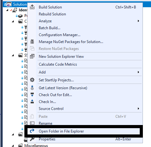
If you are using Visual Studio 2017, you can get to the directory of the solution by right clicking the solution, and choosing Open Folder in File Explorer which will get you close to the files, but you still need to navigate and find the file:

This was not in Visual Studio 2015, which is what we had been using until recently.

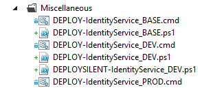
But I want to just run the file right from the Miscellaneous folder. For example the _DEV files in this directory will build/deploy the project in our DEV environment:

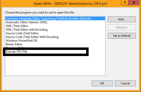
By default, if you double click the file, it will take you to edit the file in a Visual Studio editor, which is actually what is desired. I don’t want to accidentally kick off a release to DEV, much less to our PROD servers. Normally if I am clicking on a file, and making changes. But when I want to test the file, it is easiest if it can be done right from here. If you right click a .PS1 file, you can open the file in the Powershell ISE (Integrated Scripting Experience… I looked it up just for this blog!). This works, but my goal is to just execute the file.

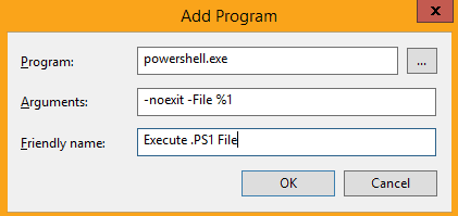
Another way to do this is to set up an “Open With…” action. For PowerShell if you right click the file, we will set up an option to run the file directly. After you click “Open With…”, click the Add button. Then fill in the blanks in the following form:

I included -noexit because I always want the file to not close the window when the file completes, so I can look over the output easily. Note that you cannot make changes to the Add Program setup if you get it wrong, but you can delete it and re-create it if it doesn’t work as you expect. Now, when you right click the file, and choose “Open With…” and choose the item we just added:

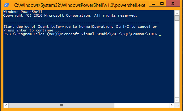
Then just choose that item and the PowerShell window will appear:

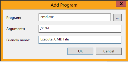
For .CMD files, which does not have an integrated scripting environment to test your code, instead of powershell.exe, use “cmd.exe” and “%1”, thusly:

Now, right click, chose “Open With…” and pick “Execute .CMD File “ and the .cmd file will start. Note that if you want it not to automatically end, you will need to include a PAUSE command.


The post Running a .PS1 or .CMD file from Visual Studio Project Explorer appeared first on Simple Talk.


from Simple Talk https://ift.tt/2BXk0gG
via