Modeling Time

Time is an interesting thing. It moves in only one direction; it’s units of measurement are irregular and constantly in motion. When we go to model it in SQL, it’s usually easier to do lookup tables (calendars) rather than trying to compute it. SQL is not a computational language, but it also must deal with the nature of this dimension. Digital computers are based on discrete states, but time by its very nature is a continuum. In a continuum, there is always an infinite number of points between any two points in the continuum. This means we’re already in a state of heresy when we try to put time into a digital computer.

Quantum Models

The quantum model is the simplest model, and a timestamp is the most common example. We simply ignore the inconvenience of the continuum and assume that time comes in discrete units or quanta. These quanta are sometimes called “chronons” in the literature. If you want to have a physical instrument for this model, think of a wall clock whose hands jump from one number to another, without sweeping in between them on the face of the clock. Or think about a calendar, whose unit of granularity is a day.

If you are a fan of kids’ television shows, you might have seen an iCarly episode that featured a new integer between 5 and 6, called “derf.” The same gimmick was recently used in an episode of DUST, a science fiction series on YouTube, if you do not to want to admit you watch kids’ television shows. Whether you treat the idea as joke or a scary fantasy, the point is that a temporal model has to be based on discrete values without gaps and a strong ordering for computations.

But what happens when you have to record a temporal value from the real world which is between quanta with such a scale? You have to assign or ignore a temporal value that is in the set of allowed values. In the Orient, a person’s age in years is a count of the full and partial years that they have lived. A new-born baby is one year old in this system. In the Western world, we only count the full years and use “months” if the child has lived less than a year. Or, to put it another way, you can round a temporal value toward the past or toward the future to map it to a quanta value in this model.

The old DATETIME data type in Transact-SQL defines a date that is combined with a time of day with fractional seconds that is based on a 24-hour clock. The date range is from 1753 January 1 to 9999 December 31. The start date is the beginning of the Gregorian calendar when it was first adopted in Great Britain. The end date is the largest four-digit year that can be represented on it. Other countries adopted it latter times, often years later (for a very detailed history, read THE CALENDAR by David Ewi ng Duncan, ISBN 9781857029796). Today we’re not really on the Gregorian calendar anymore. We use what’s called the Common Era calendar and we’ve replaced A.D. and B.C. with CE and BCE. It’s almost like the Gregorian calendar, except it starts at 0001-01-01 and goes through 9999-12-31.

The time range is 00:00:00 through 23:59:59.997, but the fractional seconds are weird. They are rounded to quanta of 0.000, 0.003, or 0.007 seconds. The reason for this has to do with the original implementation of SQL Server under Sybase. DATETIME data was stored in the floating-point format available on the original 16-bit hardware. The mantissa held the date portion, and the exponent held the clock portion. This is why if you look at old SQL Server code you may find a DATETIME value CAST or CONVERTed to floating-point, manipulated and then cast back to DATETIME. If this sounds like a kludge, that’s because it is. But it was a very fast kludge, especially if your machine had floating-point hardware. Since we had no separate DATE and TIME data types, the convention was to fake having a DATE by setting the time portion to 00:00:00.000. You will find a lot of old code for this in legacy systems.

SQL Server has had ANSI/ISO compliant date and time datatypes for several years now. You should not ever use the old DATETIME data type, and instead you should be moving on to DATETIME2(n) and DATE datatypes today. I also think it’s probably a good idea to go through and replace those old kludges with the modern datatypes. The new datatypes are not only ANSI/ISO 8601 conformant but use less storage and have more precision if you really need it. Let’s be honest, most of the time, commercial work is quite happy with precisions to a date or to a fraction of an hour within the date. While it’s nice to be able to go down to nanoseconds, we really don’t use that degree of precision in any common application you will ever run into.

Another advantage is using the ISO 8601 format which is an international standard with unambiguous specification. Also, this format isn’t affected by the SET DATEFORMAT or SET LANGUAGE setting. This format has several display options; SQL picked one.

Today, the ANSI/ISO SQL Standards only allow the ISO 8601 format which looks like “yyyy-mm-dd HH:mm:ss.ssssss”, in the language. Please notice the use of dashes and a space between the date and the time fields. The ISO 8601 standard also specifies a version that drops out the dashes and replaces the space with a “T” as a separator, which SQL Server also allows. Frankly I like the second version better because of the continuous string with no worries about white spaces (Blank? Tab? Newline? Carriage return?) and I’m very glad to see that Microsoft supports it. However, we picked the first version when we were setting up the standards because it looks nicer for people. It is the default in the SQL world.

Other Date Displays

Probably the most esoteric way of representing a date is the Julian system. It’s used by astronomers and it has nothing to do with the Julian calendar. Nobody ever uses that outside of the sciences. The count starts with 4713, January 01 BCE, and the Julian Date for 00:30:00.0 UT January 1, 2013, is 2 456 293.520 833. For details see this article and this one.

Another common way of displaying a date is simply the ordinal date format. It consist of “yyyy-ddd” where the “yyyy” is the usual year and “ddd” is the day within the year, taking on the values 001 thru 365 or 366.

Closed Interval Models

Another model is based on a closed interval defined by (start_timestamp, end_timestamp) pairs that mark the end points of a temporal interval. We assume (start_timestamp ≤ end_timestamp). All of the temporal points in the interval are assumed to be in the set of values, even if you cannot actually represent them with your software. The FIPS (Federal Information Processing Standards) require at least four decimal places of seconds in a timestamp in all clocks used by the US government. However, the current hardware and SQL Standards can give seven decimal places, nanoseconds.

A calculus for temporal reasoning was introduced in 1983 by James F. Allen (“Maintaining knowledge about temporal intervals”, Communications of the ACM. 26(11): 832–843.). It was not designed for SQL, but for general use when describing events. The following 13 base relations capture the possible relations between two intervals in Allen’s Interval Algebra:

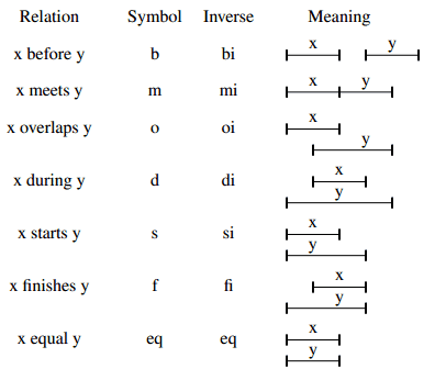
The inverse of a relation simply flips the right and left sides of the infixed operators and rewords the definition. Obviously, equality is its own inverse.

In general, the number of different relations between n intervals is 1, 1, 13, 409, 23917, 2244361… OEIS A055203. The special case shown above is for n=2.You have to decide if endpoints are co-located, or merely tangent. It gets messy, but it is a consistent, known model.

ISO Half Open Interval Model

The ISO model of time is based on half open intervals. That means we have a starting point, but we have no ending point for an interval. The duration in the interval approaches but never actually reaches the ending point. To make this a little more explicit, consider a day. It begins at 00:00:00 Hrs (midnight), progresses through 24 hours, but never gets to 24:00:00 Hrs. That final endpoint actually belongs to the start of the next day. DB2, other SQL products, and international conventions will convert 24:00:00 Hrs to midnight of the next day automatically.

Depending exactly in what precision your times are kept, you can get as close as 23:59:59.9999999 Hrs, assuming that you’re following the precision required by Federal Information Processing Standards. In actual practice, for commercial purposes, you probably are not paying your employees by the nanosecond. Let’s be honest, to be within one minute is probably good enough in most cases.

The advantage of the half open interval model is that two time periods can be abutted to each other. Each point in time belongs to one and only one interval. If you used closed intervals, then they would abut on at least one point, or could overlap. This makes for a lot of problems when you are trying to determine during which shift a particular billable event occurs.

In mathematics, this is called the partitioning of a set, and it’s where we get the name of the PARTITION BY clause in SQL. But unlike mathematics, SQL (or any other digital representation in a computer) can’t actually be a continuum. To give you an idea where I’m going, let’s assume that a day is broken into three shifts in a factory for purposes of timecards.

CREATE TABLE Shifts
(
    shift_code CHAR(12) NOT NULL PRIMARY KEY 
       CHECK (shift_code IN ( 
         'first_shift', 'second_shift', 'third_shift' )),
    start_time TIME(0) NOT NULL,
    end_time TIME(2) NOT NULL,
    CHECK (start_time < end_time)
);
INSERT INTO Shifts
VALUES
('first_shift', '09:00:00', '16:59:999'),    ---nine to five
('second_shift', '17:00:00', '19:59:999'),   ---five to eight
('third_shift', '20:00:00', '23:59:59.999'); -- graveyard shift
CREATE TABLE Timecards
(
    emp_name VARCHAR(25) NOT NULL PRIMARY KEY,
    clock_in_time TIME(0) NOT NULL,
    clock_out_time TIME(0) NOT NULL,
    CHECK (clock_in_time <= clock_out_time)
        ...
);

This is a pretty skeletal timecard system created for illustrating the basic principles of this article. A real schema would have a lot more details.

For example, employee A enters a time in/out block 08:30:00– 17:30:00. That block would have to be parsed as something like

SHIFT CODE third_shift = 0.5 hours

SHIFT CODE first_shift = 8 hours

SHIFT CODE second_shift = 0.5 hours

We can use decimal representation for hours… common in payroll and time tracking. Many decades ago, I had a similar problem. We rounded the durations to 15 minute blocks (xx:00:00 thru xx:14:59, xx:15:00 thru xx:29:59, xx:30:00 thru xx:44:59, xx:45:00 thru xx:59:59) as per union rules. 24 hrs per day * 4 blocks per hour = 96 blocks per day, 5 days per work week = 480, 50 work weeks per year = 24,000; a decade of lookups = 240,000 rows. Put a running total of blocks in each row, then subtract the starting block count from the ending block count.

We found that a simple lookup table was easier than trying to do temporal math. After all, SQL is a data language, not a computational language. Use a spreadsheet and load the table, so you are done for a decade.

The OVERLAPS() Predicate

ANSI/ISO Standard SQL defines the OVERLAPS() predicate as the result of the following expression:

(S1 > S2 AND NOT (S1 >= T2 AND T1 >= T2))

OR (S2 > S1 AND NOT (S2 >= T1 AND T2 >= T1))

OR (S1 = S2 AND (T1 <> T2 OR T1 = T2))

where S1 and S2 are the starting times of the two time periods and T1 and T2 are their termination times. The rules for the OVERLAPS() predicate sound like they should be intuitive, but they are not. The principles that we wanted in ANSI/ISO Standard SQL were:

1. A time period includes its starting point but does not include its end point. We have already discussed this temporal model.

2. If the time periods are not “instantaneous”, they overlap when they share a common time period.

3. If the first term of the predicate is an INTERVAL and the second term is an instantaneous event (a <datetime> data type), they overlap when the second term is in the time period (but is not the end point of the time period). That follows the half-open model.

4. If the first and second terms are both instantaneous events, they overlap only when they are equal.

5. If the starting time is NULL and the finishing time is a <datetime> value, the finishing time becomes the starting time and we have an event. If the starting time is NULL and the finishing time is an INTERVAL value, then both the finishing and starting times are NULL.

Please consider how your intuition reacts to these results, when the granularity is at the YEAR-MONTH-DAY level. Remember that a day begins at 00:00:00 Hrs.

(today, today) OVERLAPS (today, today) = TRUE

(today, tomorrow) OVERLAPS (today, today) = TRUE

(today, tomorrow) OVERLAPS (tomorrow, tomorrow) = FALSE

(yesterday, today) OVERLAPS (today, tomorrow) = FALSE

Keeping Contiguous Events

Alexander Kuznetsov wrote this programming idiom for History Tables in T-SQL, but it generalizes to any SQL. It builds a temporal chain from the current row to the previous row with a self-reference. This idiom easy to use, once the DDL is in place.

This is easier to show with code:

CREATE TABLE Tasks
(
    task_id INTEGER NOT NULL,
    task_score CHAR(1) NOT NULL,
    previous_end_date DATE, -- null means first task
    current_start_date DATE
        DEFAULT CURRENT_TIMESTAMP NOT NULL,
    CONSTRAINT previous_end_date_and_current_start_in_sequence 
       CHECK (previous_end_date <= current_start_date),
     --DEFERRABLE INITIALLY IMMEDIATE,
    current_end_date DATE,  -- null means unfinished current task
    CONSTRAINT current_start_and_end_dates_in_sequence 
       CHECK (current_start_date <= current_end_date),
    CONSTRAINT end_dates_in_sequence 
       CHECK (previous_end_date <> current_end_date),
    PRIMARY KEY (
                    task_id,
                    current_start_date
                ),
    UNIQUE (
               task_id,
               previous_end_date
           ),               -- null first task
    UNIQUE (
               task_id,
               current_end_date
           ),               -- one null current task
    FOREIGN KEY (
                    task_id,
                    previous_end_date
                ) -- self-reference
    REFERENCES Tasks (
                         task_id,
                         current_end_date
                     )
);

Well, that looks complicated! Let’s look at the code column by column. Task_id explains itself. The previous_end_date will not have a value for the first task in the chain, so it is NULL-able. The current_start_date and current_end_date are the same data elements, temporal sequence and PRIMARY KEY constraints we had in the simple history table schema.

The two UNIQUE constraints will allow one NULL in their pairs of columns and prevent duplicates. Remember that UNIQUE is NULL-able, not like PRIMARY KEY, which implies UNIQUE NOT NULL.

Finally, the FOREIGN KEY is the real trick. Obviously, the previous task must end when the current task started for them to abut, so there is another constraint. This constraint is a self-reference that makes sure this is true. Modifying data in this type of table is easy but requires some thought. The foreign key reference is to be disabled when this table is first constructed and then restarted afterwards. In ANSI/ISO Standard SQL, this is done with deferrable constraints, but in T-SQL you have to explicitly turn the constraint on and off during the session.

DATETIMEOFFSET

DATETIMEOFFSET is a data type giving you the ability to work with time zones. Here’s the format:

YYYY-MM-DD hh:mm:ss[.nnnnnnn] [{+|-}hh:mm]

The final option on this date format is the number of hours and minutes that the time zone difference differs from UTC. Time zones can be a little crazy, usually for political reasons rather than computational considerations. For example, for many years Japan and Korea had different zones. Columbia did not want to be in the same time zone as United States when Caesar Chavez was their dictator. You can find the currently recognized time zones here. SQL Server doesn’t care if the time zone offset exists in the real world or not, it just needs to be computationally valid.

To generate the current local non-offset date and time value in the target SQL Server instance, you use functions such as SYSDATETIME (returns DATETIME2) or GETDATE (returns DATETIME). To generate the current local date and time value with the offset, use SYSDATETIMEOFFSET. This example returns the date and time, including the offset, for US Central Standard Time when running on my computer:

PRINT SYSDATETIMEOFFSET();

This command returns:

To return the current time zone offset, you use functions like DATENAME (returns a string with hours and minutes offset) or DATEPART (returns an integer with minutes offset) with the TZoffset part (tz in short). The displacement will make allowances for daylight saving time, according to Microsoft conventions. Here’s an example which returns -300 since the offset is -5 hours:

DECLARE @Date DATETIMEOFFSET = SYSDATETIMEOFFSET();
PRINT DATEPART(tz,@Date);

AT TIME ZONE

The AT TIME ZONE function was introduced in SQL Server 2016. It replaces both TODATETIMEOFFSET and SWITCHOFFSET. It has the following syntax:

<value> AT TIME ZONE '<standard time zone name>'

Here’s an example:

DECLARE @Date DATETIMEOFFSET = GETDATE();
PRINT @Date;
SET @Date = @Date AT TIME ZONE 'Pacific Standard Time';
PRINT @Date;

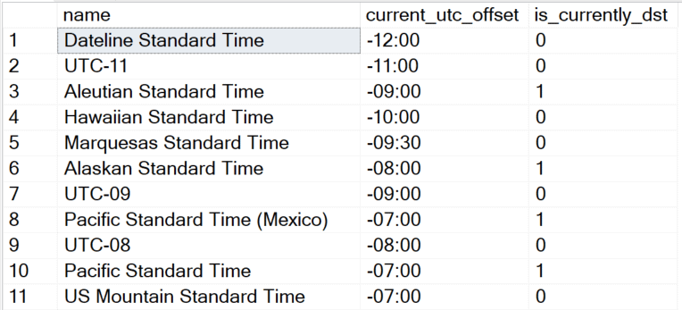
When the input value is a nonoffset date and time value, the function behaves similar to TODATETIMEOFFSET; when the input value is a date and time value with an offset, the function behaves similar to SWITCHOFFSET. Moreover, you don’t need to worry about clock switching; rather, just specify the target standard time zone name (for instance, for Pacific Time always specify ‘Pacific Standard Time’), and SQL Server will figure out dynamically the target time zone offset based on the Windows time zone conversion rules. To get the full list of supported standard time zone names, plus their current offset from UTC and whether it’s currently on daylight saving time, query the sys.time_zone_info function:

SELECT * FROM sys.time_zone_info;

The query returns 139 rows, but here is a sample:

I also strongly recommend that you read this article, so have some idea just how complicated things can get.

The Most Important Thing to take Home from this article

Use the TIME, DATE, DATETIME2 and DATETIMEOFFSET data types for new work. These types align with the SQL Standard. They are more portable. DATE, TIME DATETIME2 and DATETIMEOFFSET provide more decimal seconds precision. DATETIMEOFFSET provides time zone support for globally deployed applications, but think in UTC.

 

The post Modeling Time appeared first on Simple Talk.

from Simple Talk https://ift.tt/2LVOs0m
via

Introduction to DevOps: The Application Delivery Pipeline

The series so far:

1. Introduction to DevOps: The Evolving World of Application Delivery
2. Introduction to DevOps: The Application Delivery Pipeline

DevOps is both a mindset and a software development methodology. As a mindset, DevOps is about communication, collaboration, and information sharing. As a methodology, it’s about merging development and operations into a unified, integrated effort. At the heart of the DevOps methodology is the application delivery pipeline, which drives the development and deployment processes forward throughout the application lifecycle.

This article is the second in a series about DevOps. In the first article, I introduced you to many of the basic concepts typically associated with DevOps, including a brief discussion about the DevOps process flow. In this article, I continue that discussion with an explanation of the technologies that make up the application delivery pipeline—the underlying structure that supports this flow.

Introducing the Application Delivery Pipeline

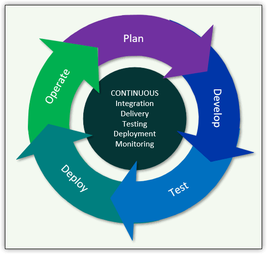
DevOps unifies the application delivery process into a continuous flow that incorporates planning, development, testing, deployment and operations, with the goal of delivering applications more quickly and easily. Figure 1 provides an overview of this delivery flow and its emphasis on continuous, integrated services.

Figure 1. The continuous services of the DevOps methodology

The continuous services—integration, delivery, testing, deployment, and monitoring—are essential to the DevOps process flow. Before I go further with this discussion, however, I should point out that documentation about DevOps practices and technologies often vary from one source to the next, leading to confusion about specific terms and variations in the process flow. Despite these differences, the underlying principles remain the same—development and operations coming together to optimize, speed up and in other ways, improve application delivery.

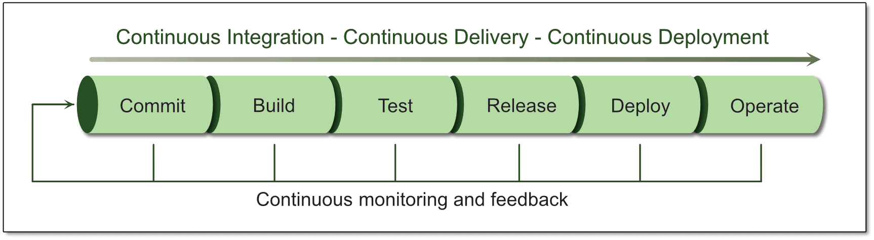
With this in mind, consider the application delivery pipeline that drives the DevOps process flow. One way to represent the pipeline is to break it down into six distinct stages—Commit, Build, Test, Release, Deploy, and Operate. The pipeline begins with code being committed to a source control repository and ends with the application being maintained in production, as shown in Figure 2. Notice that beneath the pipeline is a monitoring and feedback loop that ties the six stages together and keeps application delivery moving forward while supporting an ongoing, iterative process for regularly improving the application.

Figure 2. The DevOps application delivery pipeline

You’ll find plenty of variations of how the pipeline is represented, but the idea is the same: to show a continuous process that incorporates the full application lifecycle—from developing the applications to operating them in production. What the figure does not reflect is the underlying automation that makes the process flow possible, although it’s an integral part of the entire operation.

Also integral to the pipeline are the concepts of continuous integration (CI), continuous delivery (CD), and continuous deployment (CD). My use of the same acronym for both continuous delivery and continuous deployment is no accident. In fact, it points to one of the most common sources of confusion when it comes to the DevOps delivery pipeline.

You’ll often see the delivery process referred to as the CI/CD pipeline, with no clear indication whether CD stands for continuous delivery or continuous deployment. Although you can rely on CI referring to continuous integration in this context, it’s not always clear how CI differs from the two CDs, how the two CDs differ from each other, or how the three might be related. To complicate matters, the terms continuous delivery and continuous deployment are often used interchangeably, or one is used to represent the other.

To help bring clarity to this matter, I’ll start by dropping the use of acronyms and then give you my take on these terms, knowing full well you’re likely to stumble upon other interpretations.

I’ll start with continuous integration, which refers to the practice of automating application build and testing processes. After developers create or update code, they commit their changes to a source control repository. This launches an automated build and testing operation that validates the code whenever changes are checked into the repository. (The automated testing includes such tests as unit and integration tests.)

Developers can see the results of the build/testing process as soon as it has completed. In this way, individual developers can check in frequent and isolated changes and have those changes verified shortly after they commit the code. If any defects were introduced into the code, the developer knows immediately. At the same time, the source control system might roll back the changes committed to the central repository, depending on how continuous integration has been implemented.

With continuous integration, development teams can discover problems early in the development cycle, and the problems they do discover tend to be less complex and easier to resolve.

The CD Conundrum

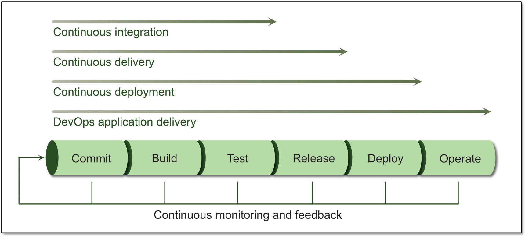
Continuous integration is often associated with the Commit, Build, and Test phases of the application delivery pipeline. Continuous delivery takes the application delivery process one step further by adding the Release stage, which is where the application is prepared and released for production. The Release stage includes test and code-release automation that ensures the code is ready for deployment. As part of this process, the code is compiled and delivered to a staging area in preparation for production.

Like continuous integration, continuous delivery is a highly automated process that allows application updates to be released more frequently. In some documentation, continuous delivery is considered a replacement for continuous integration, incorporating the integration operations into its workflow. In other documentation, continuous delivery is treated an extension of continuous integration, with one building on the other. In either case, the results are the same.

Continuous deployment moves the DevOps pipeline one step further by incorporating the Deploy phase into the delivery process. Continuous deployment presents the same muddle as continuous integration and continuous delivery; that is, continuous deployment is sometimes described as a replacement for the other services or as an extension to them. Once again, the results are the same, only this time, the pipeline’s capabilities are extended in order to automatically deploy the application to production.

In continuous delivery, an application is automatically staged in preparation for production, but it must be manually deployed to production. Before that, however, the application must be manually reviewed and verified, which can represent a significant bottleneck in the software release cycle.

Continuous deployment addresses this issue by adding automation to the equation, making it (theoretically) possible for changes to go live within minutes after the code has been checked into the repository and verified by the automated processes.

The flipside of this is that continuous deployment also eliminates the safeguards that come with manual verifications. For this reason, application delivery teams that implement continuous deployment must be certain to adhere to best coding and testing practices to ensure the application is production-ready.

Figure 3 helps to distinguish between the three continuous services, showing how each service addresses one more step on the pipeline. The figure also shows DevOps application delivery in its entirety in order to stress the importance of viewing the process as one continuous workflow, no matter how you break down or label the services.

Figure 3. The continuous services in the application delivery pipeline

As with the other figures in this article, Figure 3 is meant only to provide a conceptual overview of the application delivery process. No doubt you’ll find many variations on this theme.

Automation and Monitoring

Regardless of how you define or categorize the continuous services, what lies at the core of application delivery is a fully automated process that drives the DevOps pipeline from development through production.

Automation makes it possible to release application updates more easily and frequently while eliminating the need to perform the same mundane tasks over and over again. Automation also lets you easily deploy applications repeatedly, while ensuring that each task in the delivery process is performed correctly.

Just as important as automation is the need for continuous monitoring and feedback at every stage of the DevOps pipeline. Monitoring and feedback are essential to improving the application as well as the delivery process itself. Monitoring also makes it possible to track application usage, performance, and other metrics, while ensuring that any issues that do arise are caught and resolved as quickly as possible.

DevOps-Friendly Technologies

Today’s application development strategies incorporate several technologies that go hand-in-hand with the DevOps methodology. Three particular important technologies are containerization, microservices, and infrastructure as code (IaC).

Containerization refers to the process of implementing applications within containers. A container is similar to a virtual machine (VM) in terms of providing an environment for running applications separately from the host operating system (OS). However, the container is more lightweight and portable than the VM. Each container is packaged with all the essential runtime components, such as files and libraries, but only what is necessary to host an application. A container does not contain the entire OS like a VM.

Containers let you deploy applications in small, resource-efficient packages that can run on any machine that supports containerization, eliminating many of the dependencies that come with deploying traditional applications. Containerized applications also boot and run faster than traditional applications, requiring less of the host’s resources. At the same time, they’re highly scalable, making them well suited to the continuous delivery and deployment models.

Microservices is an application architecture for breaking an application down into small, reusable services. Each service performs a specific business function, communicating with the other services through exposed APIs (typically standards-based REST APIs). At the same time, the services remain independent from each other, which means a service can fail without bringing down the entire application. You can easily integrate microservices into your DevOps process flow because of their flexibility, scalability, and function-specific packaging.

IaC is particularly well suited to the DevOps era. In fact, many consider DevOps to be an essential component of the DevOps application delivery process, helping to ease the development effort, while better preparing the applications for production. With IaC, it’s also quick and easy to set up multiple environments that share the same configuration.

To implement IaC, you can create scripts that define the deployment environments for your applications. For example, you can determine how to configure networks, load balancers, VMs, or other components, regardless of the environment’s initial state. In this way, you can ensure that all your development and test environments properly mimic the production environment.

I should also add that cloud computing can be an important DevOps ally. The cloud provides the type of flexibility and elastic scalability that is so well suited to the DevOps approach. For example, an organization might use cloud storage to support their DevOps infrastructure because it can be quickly and automatically provisioned and scaled as application requirements change.

DevOps Tools

Organizations that plan to adopt the DevOps methodology require a number of tools. One of the most important is a source control solution for maintaining file versions. Solutions such as Git, GitHub, or Subversion let you perform such tasks as track changes, roll back commits, and compare file versions. An effective source control solution also allows developers to check in code from any location, while enabling collaboration between them.

You’ll also need tools for managing and automating the various operations that make up the application delivery pipeline. For example, you’ll require tools that continuously build, test, and deploy your code. One such tool is Jenkins, an open source automation server that lets you automate a wide range of pipeline tasks.

Most applications must have a way to store data, and often it is in SQL Server. Since a production database cannot easily be replaced like a service or application files, database changes are often a bottleneck in bringing new application features online. Consider a tool such as Redgate’s SQL Change Automation, which can bring the database into the DevOps pipeline. With full PowerShell support, it is compatible with automation tools like Jenkins.

You might also benefit from a project management tool such as Apache Maven, which follows the project object model (POM) for managing a project’s build, reporting and documentation. In addition, you’ll likely need a unit testing framework such as JUnit, NUnit, TestNG, or RSpec or an acceptance testing tool such as Calabash, Cucumber, or Fitness.

Another consideration is what tools you need to manage infrastructure. For example, you might require a configuration management tool such as Chef, Puppet, or Ansible to support your IaC deployments. These tools integrate with the process flow to let you provision and configure infrastructure components at scale. You might also need a containerization tool such as Docker or a container orchestration tool such as Kubernetes.

When considering tools, also take into account your monitoring requirements. For example, Nagios lets you continuously monitor your system, network, and infrastructure for performance and security issues. An effective monitoring solution should be able to alert you to problems when they occur, find the root causes of those problems, and help you optimise your systems and plan for infrastructure.

The DevOps Application Delivery Pipeline

When preparing to implement the DevOps methodology, you should assess the tools you have on hand to determine which ones, if any, can support the application delivery process and what additional tools you might need. Be sure to take into account issues related to integration and interoperability, as well as what it will take to deploy and learn the new tools and the processes they support.

Above all, remember that DevOps is not only a methodology but also a mindset that should be adopted by everyone who participates in the process. True, they still need to learn about the logistics of application delivery and the tools it takes to support that process, but more importantly, they should understand the necessity of open communication, collaboration, and information sharing in order to ensure that the DevOps effort can succeed.

The post Introduction to DevOps: The Application Delivery Pipeline appeared first on Simple Talk.

from Simple Talk https://ift.tt/2XMbIVN
via

SQL Server 2019: Features for the Rest of Us

I was talking recently with a friend about features of SQL Server 2019 (still in CTP at the time of this writing). I thought that while Microsoft provides features that will benefit any size shop, the exciting new feature they are promoting is Big Data Clusters. This feature allows you to query data from many other sources such as HDFS right from SQL Server with T-SQL without moving that data around. We’ve had PolyBase since 2016 which also lets you do that, but the “clusters” part of the name means running SQL Server, Spark, or HDFS in containers in Kubernetes.

I can’t see small or medium companies having much interest in this feature. My friend pointed out a handful of local marketing organisations that make their money just by analysing data. They might benefit from Big Data Clusters. I agreed that, if your company is analysing large amounts of data that is not in SQL Server, this is a brilliant solution.

Since I’ve worked with companies in a variety of industries and sizes, I’m more interested in the smaller features that make SQL Server better for everyone or solve some problems that have been around for a while. One thing that has improved over the many versions is the installation options. You can now specify max memory and max degree of parallelism during installation. Microsoft even has some recommended settings for you. Of course, these are just suggestions that may need to be tweaked based on workload and other instances running on the same server.

One feature that will save hours of troubleshooting is the new truncation error message. The old message “String or binary data would be truncated” didn’t give you any information about how to find the offending value or even which table is involved. The new message “String or binary data would be truncated in table ‘%.*ls’, column ‘%.*ls’. Truncated value: ‘%.*ls’” is going to save so much time that it might seriously be considered worth the price of an upgrade.

Microsoft continues to add to the Intelligent Query Processing features started with 2017. My favourite new feature in this group is Batch Mode on Rowstore which I wrote about as a way to improve the performance of some T-SQL window functions. Some patterns that are often problematic for performance, table variables and user-defined scalar UDFs for example, benefit from Intelligent Query Processing as well. This feature group covers quite a few innovative improvements, and I can’t wait to see what the SQL Server team comes up with next!

SQL Server provides many ways of working with data, from the traditional tables and indexes to graph databases, in-memory databases, partitioned tables, JSON, and more. Each version of SQL Server brings enhancements to these features, and 2019 is no exception. An exciting new option used with CREATE INDEX is OPTIMIZE_FOR_SEQUENTIAL_KEY. This option ends last page and other hot spot contention in the B-Tree index structure. This feature can finally end the GUIDS vs identity columns as index key arguments!

There is also one feature I would never have dreamed about, much like SQL Server running on Linux starting in 2017. In 2019, you can run JAVA code in SQL Server using sp_execute_external_script! I’m curious to learn how well this will be adopted.

Be sure to keep up with all the changes and enhancements on the way with SQL Server 2019, and I’ve just mentioned a few here. There is a lot to love no matter what your size or industry!

 

The post SQL Server 2019: Features for the Rest of Us appeared first on Simple Talk.

from Simple Talk https://ift.tt/2NJsb8D
via

Using Attributes with Unity

There will be many times when you desire to make the Unity engine look and feel better to use. While you can certainly make your own extensions for your project, there are some simpler ways to get a better feeling editor. That method comes from attributes, which allow you to perform tasks such as assigning a slider to float variable or create additional context menu items. Attributes are markers that can be applied to variables, functions, or even an entire class. All it takes to use them is knowing what attribute you want and placing it in square brackets.

Several attributes will be looked at here, providing examples of where you may wish to use them. The project accompanying this will be a simple one with the focus being placed on the attributes and what effects they have. First, variable attributes will be examined, implemented, and explained. Then a quick look will be given to a function attribute, followed by class attributes. As a final note, rather than have a section dedicated to final touches and testing things out, this article will instead test out the attributes as they are implemented.

The Setup

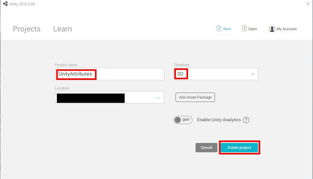
As always, the first thing to do is create the project as shown in Figure 1.

Figure 1: Creating a new project

This project will be named UnityAttributes. Select the location and set it as a 3D project. Once finished, go ahead and create the project as shown in Figure 2.

Figure 2: Naming the project and assigning its location

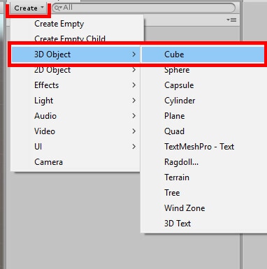
All that’s needed here is to create an object in the world. A child object will also be created and assigned the first object as its parent. Figure 3 shows how to create a Cube.

Figure 3: Creating a cube

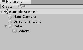
The kind of objects these will be is up to you. The example below will make the parent object a cube and the child object a sphere as shown in Figure 4. The child object will need to be given a Y position value of 1 in the inspector.

Figure 4: Setting the Sphere object as Cube’s parent.

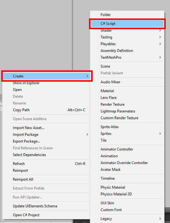
Now it’s time to create the script and start trying out some attributes. Go to the Assets window and right click. Navigate to Create->C# Script to create a new script as shown in Figure 5. This script will be called Attributes.

Figure 5: Creating a C# Script

Once ready, double click this script which opens the Visual Studio project to begin seeing what attributes can do for you.

Variable Attributes

To begin, the Update function can be deleted as it will not be used for this project. From there, the first attribute that will be looked at is Header. All you need is to feed it a string that will then display in the Inspector window. This attribute is often used the same way you might comment your code. It can also help separate categories of variables. For instance, you may have a game that asks the player to make multiple choices throughout the game, which is split into multiple days. Header would be a great way to distinguish which choices go with which in-game day. Add this code inside the class definition:

[Header("These variables will be changed a lot")]
public bool change;

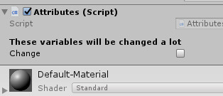
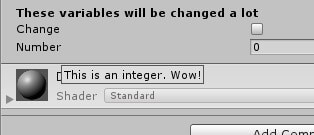
After saving the script, return to the editor, and then attach the script to the parent game object, you can see this header display in the component followed by the newly created Boolean as shown in Figure 6. Note: it may take Unity a few seconds to update the component to show this. You may also need to select a different game object then select Cube again.

Figure 6: The Header attribute in action

Similar in function, the Tooltip attribute displays a message when hovering over the variable.

[Tooltip("This is an integer. Wow!")]
public int number;

Like before, the only requirements are to assign it to a variable and give it a string. The string will be the message you wish for the tooltip to display shown in Figure 7.

Figure 7: The Tooltip attribute in action

It should be pointed out that attributes can be stacked. For instance, you can assign both a header and a tooltip to the same variable. There’s no limit to the number of attributes you can use either. In the below example, both Header and a new attribute called SerializeField are being used on the same variable.

[Header(
"This is a private variable that will be made available in the editor")]
[SerializeField]
private string firstSentence;

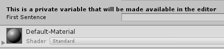
As the Header attribute points out, this private variable will be made available to edit in the inspector while maintaining its private status. Ordinarily one must make a variable public to be edited from within the Unity editor. Thanks to SerializeField, the variable firstSentence can be edited in Unity as shown in Figure 8 while also making sure no other script can touch this variable. This can be especially helpful if your project has several scripts to work with. You may still wish to change these variables outside of Visual Studio but maintain proper encapsulation, resulting in a new friend in SerializeField.

Figure 8: Demonstration of SerializeField

When using Unity, you may wish for a little room between variables. Whether this is to make the Inspector look better to you or make it harder to click the wrong thing accidentally, the Space attribute has your back. You can simply enter Space and be done, or you can enter a number to specify how many pixels of space you want.

[Space]
[SerializeField]
private string secondSentence;

Next comes an attribute perfect for variables that relate to health and other character stats or percentages that you may use. Range takes the variable it’s attributed to and gives it a slider that you can use in the Inspector. Instead of clicking inside the text box and typing a number, just take the slider and move it where you want with the mouse. But don’t think Range is exchanging anything. You still have the option to type in the variable yourself for precision.

[Space(5)]
[Header("A slider for your convenience")]
[Range(0.0f, 25.0f)]
public float newFloat;

You need only specify the minimum and maximum range for the slider. In the code above the float is given the minimum value of 0.0 and a maximum of 25.0 (the .0s specify that decimals are allowed). This also prevents you from entering a value higher than the maximum you set as shown in Figure 9.

Figure 9: Making space in Inspector and demonstrating Range

In the Inspector window, string variables are given a single line by default. You can continue typing as much as you want, but you’ll only be able to see very little of your string at once. Suppose you have a longer string you want to put in. This string could be for character dialogue or to fill in a page of an in-game book. It’s natural to want to see more than a few words. This is where TextArea comes in.

[Space]
[SerializeField]
[Tooltip("Lots of space to write")]
[TextArea]
private string longMessage;

TextArea takes the box that you normally use to type in string values in the Inspector and gives it a lot more room. You can type out long strings and still see what you’re writing. As mentioned above, something like this would be extremely helpful for moments where you have a lot of words on the screen. This has the power to make your text heavy games easier to manage.

There’s another attribute specifically used for strings. Enter Multiline, an attribute that operates similarly to TextArea.

[Space(5)]
[SerializeField]
[Tooltip("Make yourself a list")]
[Multiline]
private string listMessage;

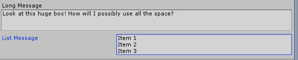
Though the functionality is very similar to TextArea, there is one key difference. When inputting something into a TextArea, the string will continue to the next line if it reaches the end of the box. Multiline, on the other hand, will continue as if it was a normal string input field. Thus, it encourages you to use Multiline for things like the list shown in Figure 10.

Figure 10: TextArea and Multiline

This next attribute has been used in previous Unity articles before but has never been given a lot of detail. HideInInspector will make your public variable hidden from the Inspector, which means you won’t be editing this value from the Unity editor. Why would you use this? In most cases, you may want a variable to be public so that other scripts can access it but don’t want any accidental edits from the editor. And of course, making it private won’t solve that problem either. So HideInInspector comes in to give you the best of both worlds.

[HideInInspector]
public bool hiddenBoolean;

The final variable attribute covered here is ContextMenuItem. Assign this attribute to a variable to add a menu option when right-clicking the variable in the Inspector. Typically, you’ll tie this menu option to a function in your script. What you’ll do in this function is up to you. In this case, the function will change the float variable to a random number between 0.0 and 5.0.

[Header("Right click this variable name!")]
[SerializeField]
[ContextMenuItem("Get a random number", "RandomNumber")]
private float randomNumber;

As you can see, the menu item is also given some text. The first string is the menu option that will appear after right-clicking the variable. Your second string is the function to perform when selecting this menu option. Speaking of which, here’s the function that this menu item will use:

void RandomNumber()
{
        randomNumber = Random.Range(0.0f, 5.0f);
}

After saving the script, you can try out the new menu option by right-clicking the variable name in the Inspector and selecting Get a random number as shown in Figure 11.

Figure 11: A user created ContextMenuItem

Function Attribute

There’s only one function attribute to discuss here, and it is similar in function to ContextMenuItem. This attribute, ContextMenu, will create a menu item when right-clicking the component instead of a specific variable. After selecting the menu option, the corresponding function will perform its task.

[ContextMenu("Do your thing")]
void NewThing()
{
        Debug.Log("I did the thing");
}

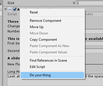
In the above example, the NewThing method is assigned the ContextMenu attribute and given a single task. You’ll see Do your thing in the menu as shown in Figure 12. When you select it, the method will print “I did the thing” to the debug log in Unity.

Figure 12: Addition made to Context menu for Attributes component

Class Attributes

Class attributes affect the entire component, not just individual variables or functions. Their functionality is quite diverse, ranging from automatically attaching additional components to the game object or making additions to Unity’s component menu. The first of these class attributes is HelpURL, which links the user to help documentation. Class attributes must be added above the class definition instead of inside the class.

[HelpURL("https://www.red-gate.com/simple-talk/dotnet/c-programming/introduction-game-development-unity-c/")]
public class Attributes : MonoBehaviour
{
        ...
}

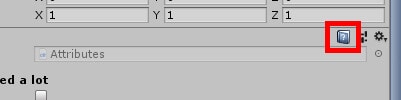
You may notice the small book icon to the right of the component in the Inspector as shown in Figure 13 window when attaching any component such as a script. If you were to click this icon, a browser window would open taking you to the documentation for that specific component. But user created scripts aren’t going to have any documentation by default, thus clicking this icon will lead to a 404 error page. After all, how can Unity Technologies hope to know what your component is doing? This is where HelpURL comes in. Give it a path to the documentation of your choosing and your user will have something to reference if they need to know how your script works. The attribute is especially useful in team projects, allowing creators to give their teammates a helping hand if needed.

Figure 13: The documentation icon

Next comes RequireComponent, and as the name implies, it forces Unity to assign whichever component you ask for. If you know that a script is going to be using specific components on the game object, this can be a helpful way to save yourself a little effort and have the script attach the required component for you. Not only that, but it also prevents anyone from removing the component from the object.

[RequireComponent(typeof (Animator))]

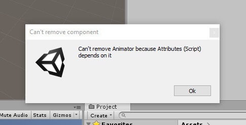
Unfortunately, you will have to either add the required component or reattach this script component to the object to see what RequireComponent can do. Once you’ve done either of those, try deleting the Animator component from the object’s Inspector and see how Unity reacts as shown in Figure 14.

Figure 14: RequireComponent disallows the removal of the Animator component

SelectionBase is the next attribute. It’s a very easy to use attribute as it requires no parameters. All you need to do is simply assign it to the class. What does this attribute do? It might seem trivial at first. This attribute will assure the user that when selecting an object from the Scene window that it will select the parent object. Why does this matter? If you have objects with several child objects attached to it, SelectionBase prevents the frustration of selecting a child object when you meant to select the parent.

[SelectionBase]

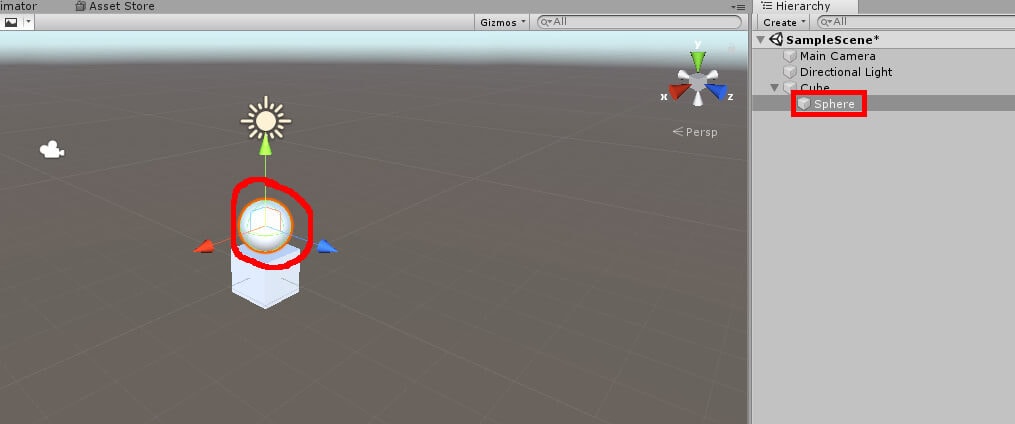
Take this very project as an example. If you were to click on the Sphere object in the Scene window, you’d find that the Sphere object is selected in the Hierarchy as shown in Figure 15.

Figure 15: Selecting an object without SelectionBase

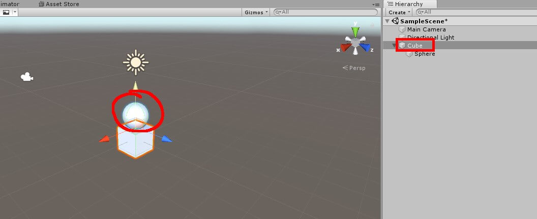
But if you attach SelectionBase to the class, the story changes. Add the attribute and save the script. Click anywhere in the Scene window to deselect the current object, then try clicking the Sphere object in the Scene window again as shown in Figure 16. Be careful not to accidentally click the movement widget as that will prevent selection of any object.

Figure 16: Selecting an object with SelectionBase. Despite clicking on the Sphere, it selected the Cube.

The Cube object was selected instead. It’s a small detail in a simpler project like this, but it can be quite the time saver in full games featuring objects with multiple child objects. Bear in mind that you can still click on the Sphere object in the Scene window and select the Sphere in the Hierarchy but only if you have the Cube object selected first. Since time-savers were mentioned, now would be a good time to look at AddComponentMenu. Once fed a path, this attribute adds to the Component menu find by selecting AddComponent in the Inspector and the Component menu in the top menu bar.

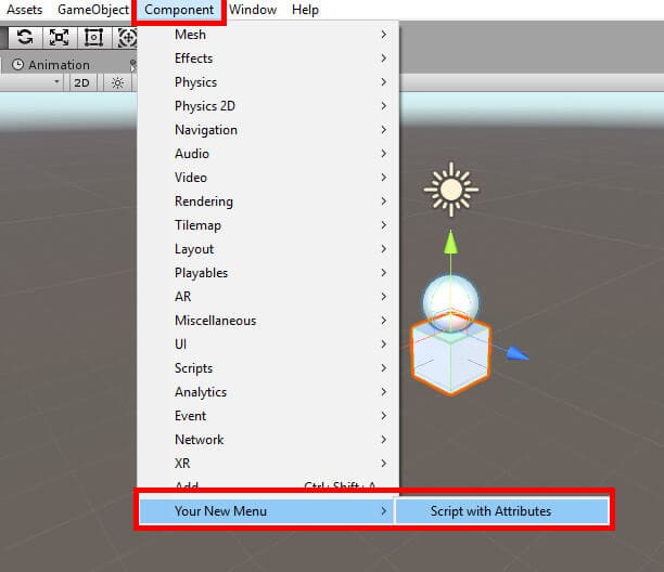
[AddComponentMenu("Your New Menu/Script with Attributes")]

In this example, a new submenu is created that has Script with Attributes added. When you select this option from the Component menu, it will attach this script, Attributes, to the game object currently selected. You can also cut out the submenu and just have the component right there in the main Component menu shown in Figure 17.

Figure 17: The AddComponentMenu attribute doing its work

The last attribute is ExecuteInEditMode, and like SelectionBase, it requires no parameters.

[ExecuteInEditMode]

When applied to a class the script will perform whatever tasks it would normally do in play mode from edit mode. For example, you can have the object change its scale or colour. Replace the Start function with this code:

void Start()
{
        GetComponent<Transform>().localScale = new Vector3(2, 2, 2);
}

There are a few things to be mindful of when using this attribute. For starters, it can add to the processing times while working in the editor. You may wish for your processor to be used towards other tasks. Also, any objects with this script will perform the actions specified. Therefore, in this example, any objects given the Attributes script component will automatically have their scale set to two as shown in Figure 18. This isn’t to say it doesn’t have any benefits of course. Some examples of good places to use ExecuteInEditMode include in editor custom warnings, position and scale constraint like in the example above, or creating required objects.

Figure 18: ExecuteInEditMode changed the scale of this object without needing to play the game

Conclusion

A lot of convenience and flexibility is offered to both you and your team when you apply attributes to your code. Variable attributes can make both your code and the Inspector window easier to manage and read. The single function attribute can do plenty to expand the editor without needing to complicated code. Finally, class attributes allow more convenience when working with objects within Unity and can even make your personal documentation easier to access for others. Before seeing the attributes in action, one may have wondered where Unity attributes would have come in handy during development. Now the question posed to developers is when they should not use attributes, and the list of reasons to not use attributes is very small indeed.

 

The post Using Attributes with Unity appeared first on Simple Talk.

from Simple Talk https://ift.tt/30hZReX
via

Reporting Services Basics: Understanding Data Sources and Datasets

The series so far:

1. Reporting Services Basics: Overview and Installation
2. Reporting Services Basics: Creating Your First Report
3. Reporting Services Basics: Data Sources and Datasets

If you’ve been following along with this series, you have learned about the architecture of Reporting Services (SSRS) and how to build a report using the wizard. Most of the time, the wizard is not that useful, although I must admit that I used the wizard for creating Matrix reports in SSRS for quite some time. In this article, you’ll begin to learn the basics of building a report from the ground up without the help of the wizard. There are two components, data sources and datasets, that you must understand to be able to build reports, so this article spends quite some time covering them.

Start with a Project

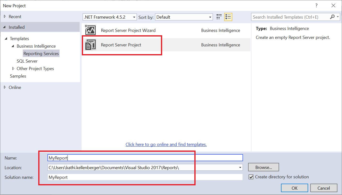
To get started, create a new Report Server Project in Visual Studio. In the previous article, you started with the Report Server Project Wizard. The Report Server Project will create the project shell without any objects. It will be up to you to add all the necessary components.

Figure 1 shows the New Project dialogue. Be sure to fill in a Name and click OK to create the project.

Figure 1: Create a new project

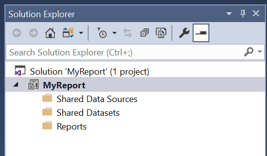
Once you create the project, you’ll see the Solution Explorer, shown in Figure 2, that is empty except for some folders.

Figure 2: The Solution Explorer

Shared Data Sources

A data source is like an address for the data. It contains the connection string. This might include the server name and stored credentials to get to a SQL Server database or be something as simple as the location of a text file. You can use multiple data sources in a report if the data will come from more than one place.

You can store data sources in two ways: sharing at the project level or embedding in the individual report. My advice is always to share the data sources, especially if you will have dozens or hundreds of reports pointing to the same database. By creating shared data sources, you or the database administrator (DBA) will have fewer of them to manage once the reports are published in the Web Portal.

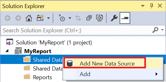
1. To get started, right-click the Shared Data Sources folder and select Add New Data Source, as shown in Figure 3.

Figure 3: Add New Data Source

1. This brings up the Shared Data Source Properties dialogue. Fill in a Name for the data source. I suggest using the database name, but your team may have a specific naming convention to use.
2. Choose the Type of database source. It’s SQL Server by default and what you’ll use in this example, but you might want to review the many sources possible.
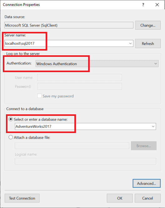
3. If you know your Connection String, you can fill it in, but it’s easier to click Edit to open the Connection Properties dialogue shown in Figure 4. You’ll need to fill in your Server name, Authentication method, and Connect to a database. (If you have problems connecting, review the Connecting to Your SQL Server Instance section in this article. If you are connecting to an instance in your network, check with your DBA for help.) Click OK to save the properties.

Figure 4: The Connection Properties

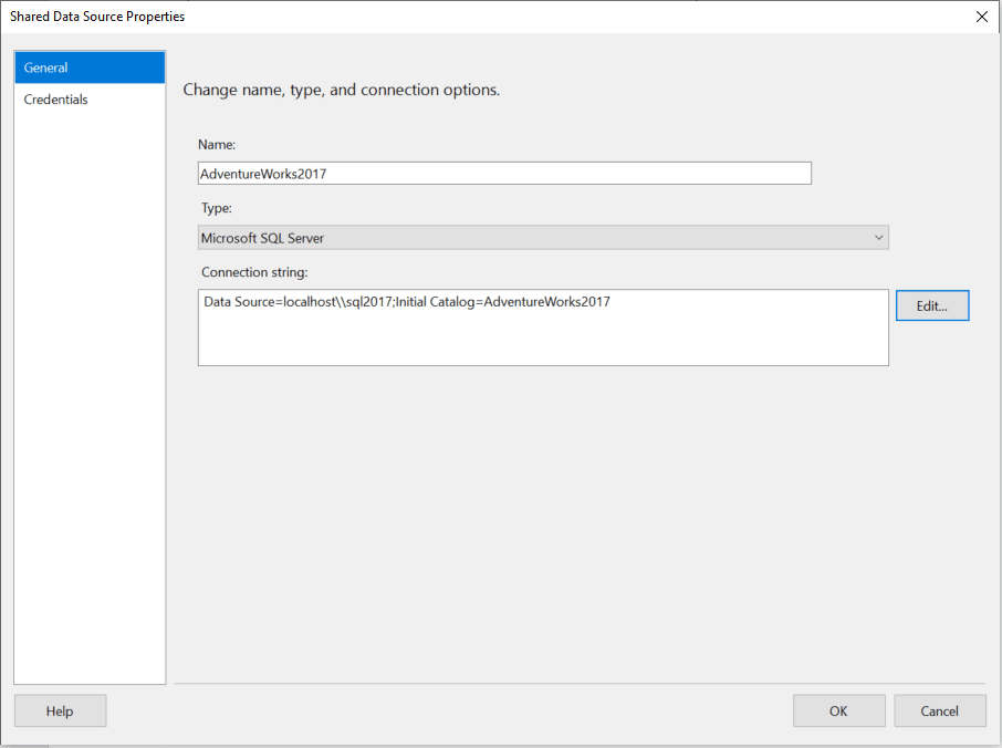
1. Once you save the properties, the General page should similar to Figure 5. Click OK to save the changes.

Figure 5: The Shared Data Source Properties

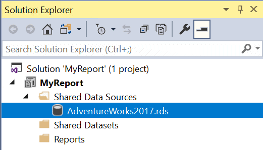
1. You’ll see the new data source in the Solution Explorer window shown in Figure 6.

Figure 6: The new data source

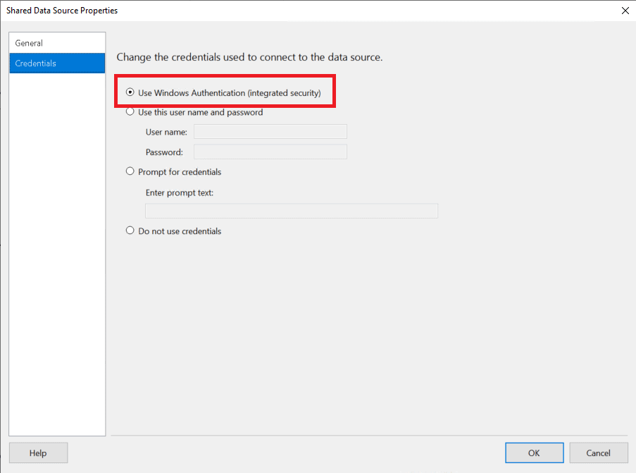
1. At the time of this writing, there is a bug that prevents saving the Credentials settings when first creating the data source. Open the properties again by double-clicking the data source. (Note that if you right-click and choose Properties, you’ll be able to see only the file location.) Figure 7 shows the Credentials page and the correct setting. Fill in the credentials that you used in Step 5 if you did not use Windows authentication. After changing the setting, click OK.

Figure 7: The data source credentials

That’s all there is to create the data source. In step 3, I pointed out that there are many different types of data sources, and configuring each type is different. For now, stick with SQL Server to get started with SSRS. View this article for more information about each type of data source.

Now it’s time to discuss datasets.

Shared Datasets

A dataset is the query that runs when you view the report. The type of query will depend on the data source. For example, when working with SQL Server databases, the query will be written in T-SQL, or you also have the option of calling stored procedures. Even though there is a Shared Datasets folder, most of the time, the dataset should be embedded in the report and not shared. The reason for embedding datasets is that queries are not reused that often. There are exceptions, for example, parameter lists that are reused in many reports. If a dataset is shared, then it will be published when you deploy the project. You probably won’t want to clutter the Web Portal with every dataset for dozens or hundreds of reports.

The report must first exist before you can embed a dataset. Instead of showing you how to create a dataset, first learn how to create a new blank report.

New Reports

When creating a new blank report, you must take care not to kick off the Report Wizard. Follow these steps to create a new blank report.

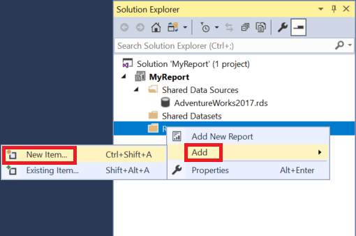
1. Right-click the Reports folder and select Add New Item…. Be sure NOT to select Add New Report, because that launches the Report Wizard. Figure 8 shows you the menu item.

Figure 8: Add new item, not add new report

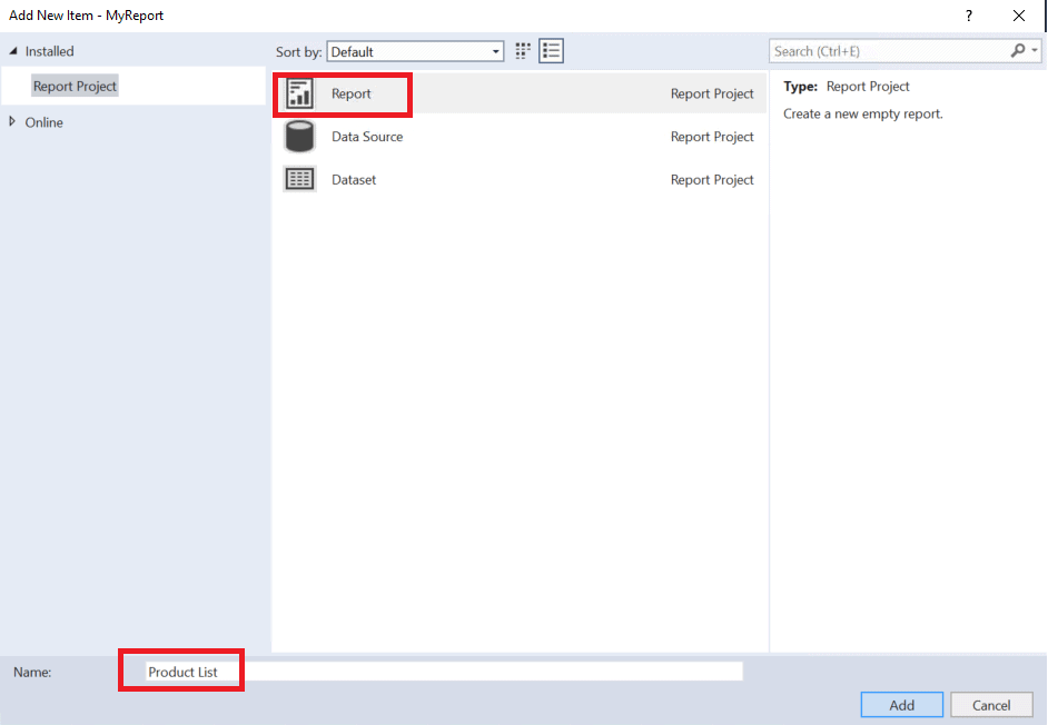
1. You’ll then see the Add New Item dialogue shown in Figure 9. Select Report and give the report a name. When working on reports for your company, be sure to provide the report with a meaningful name that will make sense to the people who run the report.

Figure 9: The Add New Item dialogue

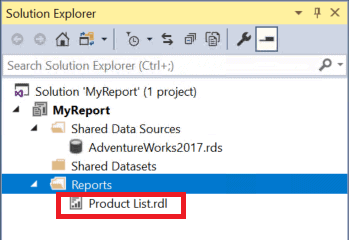
1. Click OK to create the report. You should now see it in the Solution Explorer, as shown in Figure 10.

Figure 10: View the new report

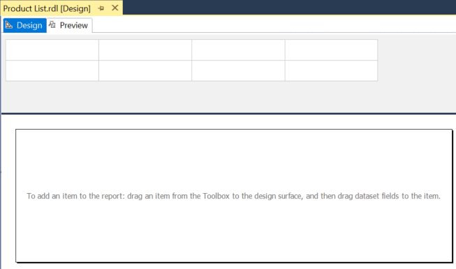
1. The new report may be open in Design view. If not, double-click it to open it. The report canvas will look like Figure 11.

Figure11: The report in Design view

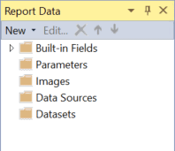
1. Now you have a new report. On the left side of the screen, you should see the Report Data window. (If you don’t see it, make sure the report canvas is selected and type CTRL+ALT+D.) Figure 12 shows you the Report Data window. Everything in this window is specific to the report you are editing. You’ll learn about the different folders throughout these articles.

Figure 12: The Report Data window

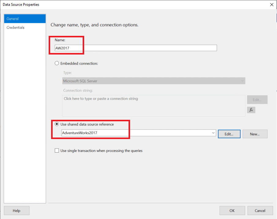
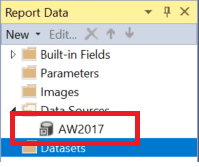
1. Right-click the Data Sources folder in the Report Data window and select Add Data Source. This data source will point to a shared reference, the data source you created earlier. Give it a Name and click Use shared data source reference. Select the AdventureWorks2017 data source from the list. (Note that you can give them the same name, but for illustration purposes, I’m naming them differently.) Figure 13 shows the properties. Click OK to create the data source.

Figure 13: The data source properties

1. Once you create the data source, you’ll see it in the window. Notice that it has a little arrow on the icon that designates that it is pointing to a shared data source, as shown in Figure 14.

Figure 14: The new data source

You now have everything in place to create an embedded dataset.

Embedded Datasets

As mentioned earlier, it makes sense to embed most datasets in the reports instead of sharing them. Shared datasets end up published as reusable Report Parts for creating ad-hoc reports by advanced users. Most datasets are not needed for this and sharing them will clutter up the folder and make it more difficult for end users to find what they need. In the later article about parameters, you’ll learn to create shared datasets when it makes sense.

Make sure that your data source pointing to the shared data source is in place and follow these steps to create a dataset.

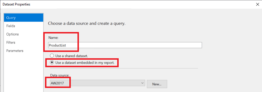
1. Fill in a Name that describes your query. Select Use a dataset embedded in my report. A dropdown box for the data source will appear. Select the data source you just created. At this point, the dialogue box will look like Figure 15.

Figure 15: The Datasets Properties so far

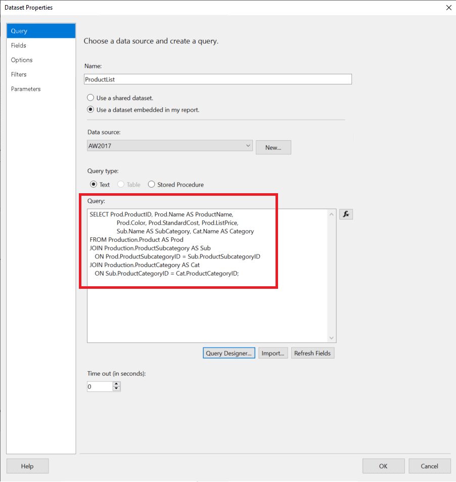
1. Make sure that the Query type is set to Text and paste in this query:

SELECT Prod.ProductID, Prod.Name AS ProductName, 
        Prod.Color, Prod.StandardCost, Prod.ListPrice, 
        Sub.Name AS SubCategory, Cat.Name AS Category
FROM Production.Product AS Prod
JOIN Production.ProductSubcategory AS Sub 
   ON Prod.ProductSubcategoryID = Sub.ProductSubcategoryID
JOIN Production.ProductCategory AS Cat 
   ON Sub.ProductCategoryID = Cat.ProductCategoryID;

1. There is also a Query Designer you can use to build simple queries, or you can import a query from a text file. I recommend writing the query in SSMS or ADS and pasting it here. The Dataset Properties should look like Figure 16. Click OK to create the dataset.

Figure 16: Paste in the query

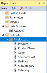
1. Once you have saved the dataset, you’ll see it along with all the fields in the Report Data window. Click the arrow next to the dataset to expand the fields, as shown in Figure 17.

Figure 17: The new dataset

If you have made any syntax errors in the query – and it’s a good practice to make sure it runs first in SSMS – the fields will not show up. To troubleshoot, you can double-click to open the properties again and fix the query. You may need to click Refresh Fields to see the change.

Adding Fields to the Report

You’ll learn much more about creating reports throughout this series, but to make sure that what you’ve done so far works follow these steps to create a rudimentary report:

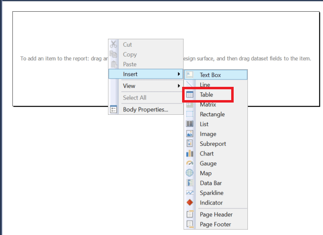
1. Right-click on the report canvas and select Insert Table as shown in Figure 18. You can also drag objects from the Toolbox window to the canvas to accomplish the same thing.

Figure 18: Insert a table

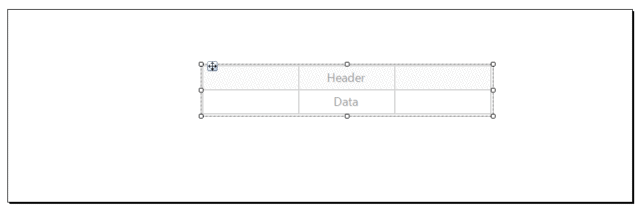
1. You’ll see a small grid with a Header and Detail row shown in Figure 19.

Figure 19: The new table

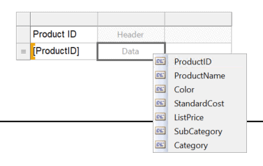
1. There are three ways to add fields to the table. You can drag them over to the Detail row from the dataset in the Report Data window. You can hover over a cell and select from the little popup menu, as shown in Figure 20. You could also type the field with brackets in the detail row, but the header will not be automatically filled in for you. If you try this last method, note that the fields are case-sensitive.

Figure 20: How to add a field to the table

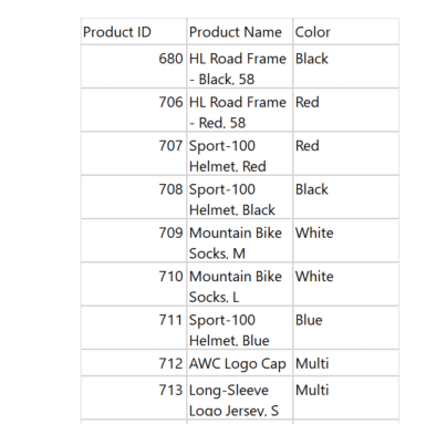
1. Now that you have added a few fields, click Preview to view the report so far. My report looks like Figure 21.

Figure 21: The report so far

Of course, there is much more work to do on this report, but this shows you that your dataset is working.

Summary

In this article, you learned how to

• Create an SSRS project
• Add a shared data source
• Add a report without launching the wizard
• Point a report data source to a shared data source
• Embed a dataset in the report
• Add a table to the report
• Add some fields to the table

I suggest that you refer to this article until you become comfortable with data sources and datasets. The concepts are confusing for many students, so having a resource you can follow will make all the difference.

The next article will build on what you know about creating reports, and you’ll get to learn about some of the other components like headers and footers that make up a report.

 

 

The post Reporting Services Basics: Understanding Data Sources and Datasets appeared first on Simple Talk.

from Simple Talk https://ift.tt/2FPaeiz
via

The End of SQL Server 2008 and 2008 R2 Extended Support

If you are not already aware, SQL Server 2008 and SQL Server 2008 R2’s extended support will end on 9 July 2019. Microsoft has communicated this end date for a while now, including this announcement with resources on how to migrate from these two versions of Microsoft SQL Server.

What This Means

Microsoft has a defined lifecycle support policy, but there are two separate policies at the time of this article. The one SQL Server 2008 and SQL Server 2008 R2 fall into is known as the Fixed Lifecycle Policy. Under this policy, Microsoft commits to a minimum of 10 years of support, with at least five years of support each for Mainstream Support and Extended Support. What is the difference between the two? What happens when Extended Support ends?

Mainstream Support

Under Mainstream Support, customers get support both for incidents (issues with the application or system) and security updates. In addition, a customer can request product design and feature changes. If there is a bug found that isn’t security related, Microsoft may choose to fix it and release an update. Microsoft has rolled up many of these fixes into service packs and cumulative updates over the years.

Extended Support

Extended Support ends the regular incident support as well as requests for product design and feature changes unless a customer has a particular support contract now called Unified Support. Microsoft will continue to release security updates but will not typically release updates for other types of bugs. SQL Server 2008 and SQL Server 2008 R2 are in the fixed lifecycle until 9 July 2019.

Beyond Extended Support

Without being part of the Extended Support Update Program, there are no more updates, security or otherwise for your organisation once extended support ends. Only if Microsoft deems that a particular security vulnerability is sensitive enough will they decide to release a patch even for systems that are now in beyond extended support status. Microsoft has released patches a couple of times for out of support operating systems, but it should not be something you count on. I will talk more about Extended Support towards the end of this article when discussing what to do if you cannot migrate from SQL Server 2008 or SQL Server 2008 R2 in time.

Compliance Requirements

Depending on what industry standard, government regulations, and laws that apply to your organisation, you may be in a situation where you will be out of compliance should you have unsupported software. This would mean you would have to participate in the Extended Support Upgrade Program, incurring the expense of that program.

Reasons to Upgrade

If you are like me, you do not have a lot of spare time to upgrade a system for the sake of it. In IT there is always more to do than there is time to do it. Microsoft discontinuing support is a reasonable justification, but I would hope to get more out of an upgrade and the resulting chaos that always accompanies such efforts than just staying in support. The good news is that by upgrading from SQL Server 2008 or 2008 R2, there are additional features that you can put to immediate use. These features do not even require touching any applications. In addition, newer versions of SQL Server include plenty of features that would require some modification but are worth considering. Here is a list of some of this new functionality:

In Memory OLTP

Once upon a time, there was the DBCC PINTABLE() command, which allowed you to keep a table in memory for better performance. That stopped with SQL Server 2005, though the command was still present in that version of SQL Server. The idea was that SQL Server’s optimisation and fetch capabilities were robust enough to keep up with demand.

Of course, this did not hold true. As a result, Microsoft researched and developed Hekaton, which is an in-memory database option. Designed from the ground up, it doesn’t function at all like the old DBCC PINTABLE() command because how the data is stored is different. If you need the performance such an option provides, it became available with SQL Server 2014.

Columnstore Indexes

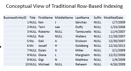
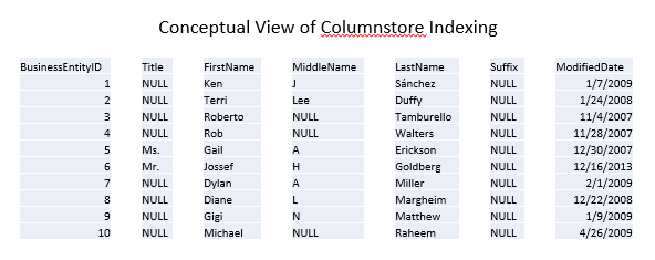
Most queries don’t require all the columns in a table. However, because a standard index is organised by row, you have to retrieve every row, and every column of every row, for each row which matches the query predicate. Conceptually, data is stored like this, with every column being kept together for a given row:

In other words, the engine is probably making a lot of extra reads to get the data you need. However, since that’s the way data is stored, you don’t have any other choice.

Columnstore indexes store the data in separate segments, one column per segment. A column can consist of more than one segment, but no segment can have more than one column. At a high level, you can think of the index working like this:

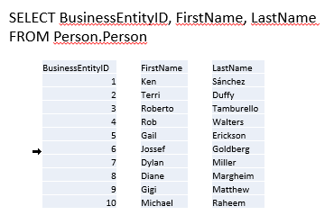
As a result, you just have to pull the segments related to the columns you care about, reading fewer pages and therefore achieving better performance. Continuing with the conceptual view, a query only wanting BusinessEntityID, FirstName, and LastName requires fewer reads because SQL Server doesn’t have to also grab data for Title, MiddleName, Suffix, and ModifiedDate simply to read in the entire row:

Columnstore Indexes are especially helpful in reporting and analytical scenarios with star or snowflake schema with a large fact table. The segmentation of the columns and the compression built into columnstore indexes means the query runs a lot faster than with a traditional index. However, this feature is not available until SQL Server 2012.

Availability Groups and Basic Availability Groups

If you have ever worked with traditional failover cluster instances, you understand the pains that this high availability (HA) option brings with it. The good news is that there is one instance, and all databases are highly available. The biggest bear of a requirement is the shared storage that all the nodes can access. This means you only have one set of the database files, and there is only one accessible copy of the data.

With a failover cluster instance, failover means stopping SQL Server on one node and starting it on another node. This can happen automatically, but during that failover, the SQL Server instance is unavailable.

With Availability Groups, introduced in SQL Server 2012, the HA is at the database level. Availability Groups do not require shared storage. In fact, Availability Groups do not use shared storage at all. This means you have more than one copy: at least one primary and from one to eight secondaries. These secondaries can be used for read-only access. In addition, there is technology that allows any of the partners (primary or secondary) to reach out to the other partners if a partner detects page-level corruption and get a correct page to replace the corrupted page. This feature is Automatic Page Repair.

Finally, with SQL Server 2016, Microsoft introduced Basic Availability Groups. Do you want the high availability but you do not need to access a secondary for read-only operations? Then you can take advantage of a basic availability group which only requires Standard Edition, therefore, it’s significantly cheaper.

Audit Object

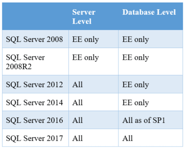
One of the easiest ways to set up auditing is with the aptly named Audit object. However, when Microsoft first introduced this feature in SQL Server 2008, Microsoft deemed it was an Enterprise Edition only feature. While you can do similar things using Extended Events (actually, the Audit object is a set of Extended Events), it is not as easy to set up.

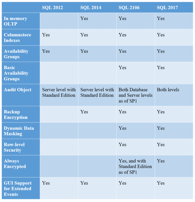
With industry’s need for auditing only growing, Microsoft has changed its stance in stages. Starting in SQL Server 2012, Microsoft enabled server-level auditing for Standard Edition. Then, in SQL Server 2016, starting with SP1, you can now use the Audit object at the database level with Standard Edition. Gaining access to Audit can be a huge benefit for compliance on our SQL Servers. I have found it helpful to have a quick chart:

Backup Encryption

When Microsoft introduced Transparent Data Encryption (TDE), it also introduced encrypted backups. However, initially, the encrypted backups were only for databases protected by TDE. TDE is an Enterprise Edition only feature. That meant you only had encrypted backups if you (a) were using Enterprise Edition and (b) had configured TDE on a particular database.

The third-party market (including Red Gate) has offered encryption in their SQL Server backup products for years. As a result, the community asked for Microsoft to also include backup encryption as a standard function for Microsoft SQL Server without having to use TDE. As a result, Microsoft added it to SQL Server 2014.

Backup encryption is crucial because smart attackers look for database backups. If an attacker can grab an unencrypted database backup, the attacker does not have to try and break into SQL Server. The attacker gets the same payoff but with less work. Therefore, if you can encrypt the database backups, especially if you belong to a firm without a third-party backup solution, you force the attackers to use a different, hopefully, more difficult method to get to the data. The more techniques an attacker must try, the more likely you are to discover the attempted hacking.

Dynamic Data Masking

I will admit to not being a fan of data masking. Solutions implementing data masking either leave the data at rest unmasked or they store the algorithm with the masked data in some form. This makes sense since privileged users must be able to see the real data. SQL Server is no different in this regard.

However, the purpose of SQL Server’s data masking is to provide a seamless solution for applications and users who shouldn’t see the actual data. You can define the masking algorithm. You can also define who can see the real data using a new permission, UNMASK. As long as you don’t change the data type/length of the field used in order to accommodate the masking algorithm, you can implement dynamic data masking without changing the application code or a user’s query unless they’re doing something to key off of the actual data.

Microsoft introduced this feature in SQL Server 2016, and its implementation can solve typical audit points around protecting the data in a system or report. As a result, it’s a great reason to upgrade from SQL Server 2008/2008R2 if you need to meet this sort of audit requirement.

Row-Level Security

You could implement row-level security solutions in SQL Server for years using views. However, there are some issues with this, as there are information disclosure issues with these home-grown solutions. The attack is basic: a savvy attacker can execute a query which reveals a bit about how the solution was built by forcing an error. A true, integrated row-level security solution was needed. As a result, Microsoft implemented row-level security as a feature first in Microsoft Azure and then in SQL Server 2016.

Speaking from experience, getting the home-grown solutions correct can be a problem. You have to be careful about how you write your filtering views or functions. Sometimes you’ll get duplicate rows because a security principal matches multiple ways for access. Therefore, you end up using the DISTINCT keyword or some similar method. Another issue is that often the security view or function is serialised, meaning performance is terrible in any system with more than a minimal load.

While you can still make mistakes on the performance side, you avoid the information disclosure issue and the row duplication issue.

Always Encrypted

When looking at encryption solutions for SQL Server, you should ask who can view the data. The focus is typically on the DBA or the administrator. Here are the three options:

1. DBAs can view the data.
2. DBAs cannot view the data but OS system administrators where SQL Server is installed can.
3. Neither the DBAs nor the system administrators can view the data.

System administrators are usually singled out for one of two reasons:

1. The DBAs also have administrative rights over the OS. In this case, #1 and #2 are the same level of permissions, meaning the DBAs can view the data.
2. The system administrators over the SQL Servers do not have permissions over the web or application servers.

If the DBAs can view the data, then you can use SQL Server’s built-in encryption mechanisms and let SQL Server perform key escrow using the standard pattern: database master key encrypts asymmetric key/certificate encrypts symmetric key encrypts data. If the DBAs cannot view the data and they aren’t system administrators but system administrators can (because they can see the system’s memory), then you can use the SQL Server built-in encryption, but you’ll need to have those keys encrypted by password, which the application has stored and uses. In either case, the built-in functions do the job, but they are hard to retrofit into an existing application, and they are not the easiest to use even if you are starting from scratch.

If neither the DBAs nor anyone who can access the system’s memory is allowed to view the data, then you cannot use SQL Server’s built-in encryption. The data must be encrypted before it reaches the SQL Server. Previously, this meant you had to build an encryption solution into the application. This is not typically a skillset for most developers. That means developers are operating out of their core body of knowledge, which means they work slower than they would like. It also means they may miss something important because they lack the knowledge to implement the encryption solution properly, despite their best efforts.

Another scenario is that you may need to retrofit an existing application to ensure that the data in the database in encrypted and/or the data in flight is encrypted. Retrofitting an application is expensive. The system is in production, so changes are the costliest at this point in the application’s lifecycle. Making these changes is going to require extensive testing just to maintain existing functionality. Wouldn’t it be great if the encryption/decryption could happen seamlessly to our application? That is what Always Encrypted does.

Always Encrypted is available starting with SQL Server 2016 (Enterprise Edition) or SQL Server 2016 SP1 (opened up for Standard Edition). Always Encrypted has a client on the application server. The client takes the database requests from the application and handles the encryption/decryption seamlessly. The back-end data in SQL Server is stored in a binary format, and while SQL Server has information on how the data is encrypted: the algorithm and metadata about the keys, however, the keys to decrypt are not stored with SQL Server. As a result, the DBA cannot decrypt the data unless the DBA has access to more than SQL Server or the OS where SQL Server is installed.

Better Support for Extended Events

Extended Events were introduced in SQL Server 2008, but they were not easy to use. For instance, there was no GUI to help set up and use Extended Events. The only way to work with Extended Events was via T-SQL.

Starting with SQL Server 2012, GUI support was introduced in SQL Server Management Studio (SSMS). With each new version of SQL Server, Microsoft extends what you can monitor with Extended Events (pun intended). The ability to capture information about new features is only instrumented with Extended Events. If you are still in “Camp Profiler,” you cannot monitor these features short of capturing every T-SQL statement or batch. That is not efficient.

One of the most important reasons to move off Profiler server-side traces and towards Extended Events is performance. The observer overhead for traces is generally higher than extended events, especially under CPU load. This is especially true using Profiler (the GUI) for monitoring SQL Server activity. Another area of performance improvement is with the filter/predicate. You can set a filter just like with Profiler. However, with Extended Events, the filtering is designed to happen as quickly as possible. SQL Server will honour the filter as it considers whether or not to capture an event. If it hits the filter, it cuts out and goes no further for that particular extended event set up. This is different than the deprecated trace behaviour. While trace will still apply the filter, it does so after the event/data collection has occurred, which results in “relatively little performance savings.” With these two improvements, Extended Events should capture only the data you specify, and it should cut out if it determines you aren’t actually interested in the event because of the filters you specified, meaning less load on the system due to monitoring.

That’s why, in the majority of cases, Extended Events are more lightweight than traditional traces. They certainly can capture more, especially if you are using any of the new features introduced from SQL Server 2012 and later. This, in and of itself, may be a great reason to migrate away from SQL Server 2008. After all, the better you can instrument your production environment while minimising the performance impact, the better.

Windowing Functions, DDL We’ve Cried For, and More, All in T-SQL

With every new version of SQL Server, Microsoft will add new features as well as improve existing ones. With SQL Server 2012, Microsoft introduced a significant amount of new functionality through T-SQL. Some of this functionality applied to queries, but others applied to configuration and database schema management. Here are three at three meaningful examples.

Windowing Functions

Window(ing) functions compute aggregations based on defined partitions. SQL Server 2008 and 2008R2 did have windowing functions using OVER() and PARTITION BY for ranking and aggregates. With SQL Server 2012 You get LAG() and LEAD(). You can also do more with aggregate functions. For instance, imagine the scenario where you had to report the order total for each order, but you also had to show the previous order total (LAG) and the next order total (LEAD). You might have another requirement, which is to show a running total. All of this can be put into a simple query:

SELECT SalesOrderID, OrderYear, OrderMonth, OrderDay, OrderTotal,
  LAG(OrderTotal, 1, 0) OVER (ORDER BY SalesOrderID) AS PreviousOrderTotal,
  LEAD(OrderTotal, 1) OVER (ORDER BY SalesOrderID) AS NextOrderTotal,
  SUM(OrderTotal) OVER (ORDER BY SalesOrderID ROWS BETWEEN UNBOUNDED PRECEDING 
                                              AND CURRENT ROW) AS RunningTotal
FROM
-- This subquery is to aggregate all the line items for an order
-- into a single total and simplify the year, month, day for
-- the query
(SELECT SOH.SalesOrderID, YEAR(SOH.OrderDate) AS 'OrderYear', 
  MONTH(SOH.OrderDate) AS 'OrderMonth', DAY(SOH.OrderDate) AS 'OrderDay', 
  SUM(SOD.LineTotal) AS OrderTotal
FROM Sales.SalesOrderDetail AS SOD
  JOIN Sales.SalesOrderHeader AS SOH
    ON SOD.SalesOrderID = SOH.SalesOrderID
GROUP BY SOH.SalesOrderID, SOH.OrderDate) SalesRawData;

The neatest function is SUM() because of the ORDER BY in the OVER() clause. Note that the query uses the keyword ROWS in the framing clause. This is new to SQL Server 2012, and the use of ROWS here tells SQL Server to add up all the rows prior to and including the current one. Since SQL Server is gathering the data at one time, the single query performs faster than having multiple queries trying to gather, re-gather, and calculate the same information. In addition, the data is all on the same row:

There are more window functions around rank distribution as well as the RANGE clause, which is similar in use to ROWS. SQL Server 2012 greatly expanded SQL Server’s window function support.

User-Defined Server Roles

When SQL Server 2005 debuted, it introduced a granular access model. A DBA could apply security to almost every object or feature of SQL Server. Microsoft pushed for the use of the new security model over the built-in database and server roles. However, at the time some server-level functionality keyed in on whether a login was in a role like sysadmin rather than checking to see if the login had the CONTROL permissions. As a result, DBAs stayed primarily with the roles that came with SQL Server.

The other issue was that SQL Server didn’t permit user-defined roles at the server level. Therefore, if a DBA wanted to implement a specific set of permissions at the server level using the granular model, that could be done, but it wasn’t tied to a role. This conflicted with the best practice of creating a role, assigning permissions to a role, and then granting membership to that role for the security principals (logins or users, in SQL Server’s case). DBAs could carry out this best practice at the database level, but not at the server level. With SQL Server 2012, server level user-defined roles are now possible. Therefore, it’s now possible to follow this best practice. However, you need to segment your permissions at the server level; you can create a role, assign the permissions, and then grant membership.

DROP IF EXISTS

A common problem DBAs face when handling deployments is when a script wants to create an object that already exists or the script wants to drop an object that isn’t there. To get around it, DBAs and developers have typically had to write code like this:

IF EXISTS(SELECT [name] FROM sys.objects WHERE name = ‘FooTable’)
  DROP TABLE FooTable;

Note that each of these statements must have the correct name. As a result, a DBA or developer putting together a deployment script updating hundreds of objects would need to verify each IF EXISTS() statement. Without third-party tools which do this sort of scripting for you, it can be cumbersome, especially in a large deployment. All that IF EXISTS() does is check for the existence of the object. Therefore, the community asked Microsoft for an IF EXISTS clause within the DROP statement that did the check and eliminated the need for this type of larger, more error-prone clause. Microsoft added this feature in SQL Server 2016. Now, you can simply do this:

DROP TABLE IF EXISTS FooTable;

If the table exists, SQL Server drops it. If the table doesn’t exist, SQL Server moves on without an error.

Ways to Migrate

Hopefully, you have gotten the go-ahead to migrate from your old SQL Server 2008/2008R2 instances to a new version. The next question is, “How?” One of the biggest concerns is breaking an existing application. There are some techniques to minimise these pains.

DNS is Your Friend

One of the chief concerns I hear about migrating database servers is, “I have to update all of my connections.” Sometimes this is followed by, “I’m not sure where all of them are, especially on the reporting side.” Here is where DNS can help.

I recommend trying to use “friendly” names in DNS that don’t refer to the server name, but to a generic name. Say there is an application called Brian’s Super Application. Rather than pointing to the actual server name of SQLServer144, you create an alias in DNS (a CNAME record in DNS parlance) called BriansSuperApp-SQL which is an alias to SQLSErver144. Then you can point the application to that friendlier name. If, at any point, the IP address on SQLServer144 changes, the CNAME will always be a reference to SQLServer144, meaning the client will get the correct IP address. Moreover, if you need to migrate to another SQL Server, say SQLServer278, simply change the alias. Point BriansSuperApp-SQL to SQLServer278, and the clients are repointed. You don’t have to change any connection information. This is an example of loose coupling applied to infrastructure.

But what if there are already applications configured to point directly to SQLServer144? Again, DNS can help. If you can migrate the databases and security from SQLServer144 to a newer SQL Server and then bring SQLServer144 off-line, you can use the same trick in DNS. Only instead of having a reference to BriansSuper-SQL that points to SQLServer278, you will delete all DNS records for SQLServer144 and then create a DNS record called SQLServer144 that points to SQLServer278. I have used this trick a lot in migrations, but it does require all the databases to move en masse to a single replacement server and the old server to be completely offline to work.

Remember Compatibility Levels

If your application requires a compatibility level of SQL Server 2008 or 2008R2, keep in mind that newer versions of SQL Server can support databases set to older versions of SQL Server via ALTER DATABASE. The compatibility designation for both SQL Server 2008 and 2008R2 is 100. All supported versions of SQL Server allow you to run a database in this compatibility mode. Therefore, you should be able to deploy to SQL Server 2017 (or 2019, if it is out by the time you are reading this).

Data Migration Assistant

What if you’re not sure if you can migrate from SQL Server 2008? Is there functionality that will break in the new version? Can you move the database to Azure? Trying to answer these questions can be a daunting task. However, Microsoft does have the Data Migration Assistant to assess your databases’ readiness to upgrade or move to Azure. Previously, DBAs would assess SQL Server Upgrade Advisor. Data Migration Assistant is extremely easy to use. First, you’ll need to create a project and tell DMA what you’re attempting to do:

In this case, the assessment is for a SQL Server to SQL Server migration (on-premises). Then, you’ll need to tell DMA what to connect to and what to assess. Once DMA has verified it can connect and access the databases you’ve chosen, you’ll indicate what you what DMA to look at:

Here, the target specified is SQL Server 2017 and DMA is being instructed to not only look at compatibility issues but also to examine any new features that might be helpful. DMA will churn away and return its assessment:

In this case, DMA noticed that Full-Text Search objects exist in the database. While DMA evaluated a SQL Server 2014 system and DB, note that DMA still flags a SQL Server 2008 issue. Like with any tool recommendations, you’ll need to consider whether the information presented applies in your case. Here, because DMA is looking at a SQL Server 2014 DB running on SQL Server 2014, there’s no issue with upgrading the database to a SQL Server 2017 instance.

Now AdventureWorks is a tiny, relatively simple database. You wouldn’t expect DMA to find much if anything. For your databases, especially large and complex ones, expect DMA to churn for a while and to have more recommendations and warnings.

What If You Can’t?

You may be in a situation where you cannot make a move by the deadline. What are your options? There are three:

Extended Security Updates

The first option, especially if you have to stay with on-premises SQL Servers, is to join the Extended Support Update program mentioned earlier. This is a pricy option, but it is the only way to maintain support for on-premises SQL Servers. Keep in mind, though, that in order to enroll in this program, Microsoft may very well ask for a migration plan on how and when you will move to supported versions of SQL Server.

Microsoft Azure

If you have the option of moving to a VM in Azure, then you will have additional coverage for three more years, as Microsoft indicated in a post on the Microsoft Azure blog. Microsoft has promised extended security updates at no extra cost if you are running on an Azure VM. In addition, the blog includes a reminder that a managed instance in Azure is another option for customers.

Again, you have to have the capability of moving to Azure. However, if you already in Azure or if you have been preparing to establish a presence, then an Azure VM may be a solution if you cannot migrate off SQL Server 2008 or 2008R2.

Go Without Support

The last option is to continue to run SQL Server 2008 or SQL Server 2008 R2 with no support. Your organisation may reason that Microsoft SQL Server has been relatively secure with only a handful of patches. There are a couple of issues, however.

The first issue is “you don’t know what you don’t know.” Someone may find a vulnerability tomorrow that is critical, easily exploitable, and which adversaries seize upon quickly. This was the case with SQL Slammer in the SQL Server 2000 days.

The second issue is around compliance. Some regulations, industry standards, and laws require systems to be running on supported, patched software. If your organisation is required to comply in such a manner, then going without support means the organisation is knowingly violating compliance and risks being caught. This is not just an immediate issue. After all, many regulations and laws can result in penalties and fines well after the period of non-compliance.

An organisation should only choose to go without support after a proper risk assessment. I know of cases where organisations decided to continue on NT 4 domains because they could not migrate to Active Directory. Other organisations have had key software that only ran on Windows 95, SQL Server 6.5, or some other ancient software. They could not find a proper replacement for that essential software and the business risk was more significant not to have the software or its functionality than running unsupported operating systems or software. However, those were informed decisions made after considering which was the greater risk.

Conclusion

With SQL Server 2008 and 2008 R2 extended support ending, it’s time to move off those database platforms. Even if you’re not required to upgrade from a GRC perspective, there’s a lot of functionality in the newer versions of SQL Server you can leverage for the benefit of your organisation. Microsoft has provided tools and guidance for upgrading. One example is the Data Migration Assistant. Microsoft has also provided additional documented guidance in SQL Docs to cover your migration scenario. If you can’t upgrade, but you require support, there are two paths you must choose from. The more costly option is to enter the Extended Support Upgrade program. The other path is to deploy to SQL Server 2008 instances in Microsoft Azure, as these will remain under support until 2022.

 

The post The End of SQL Server 2008 and 2008 R2 Extended Support appeared first on Simple Talk.

from Simple Talk http://bit.ly/2L9a60H
via