Service Pack – Fix Missing MSI issue

You know what it’s like, you are running a service pack on SQL Server and 99.9% of the time it all runs smoothly but that odd 0.1% of the time when it doesn’t is usually in the middle of the night with no one around to call on.

Well to spare you some pain I’ve discovered a really cool utility to help mitigate risk.

I was recently doing a service pack, I’d run it on the entire test estate and half of the Production estate, I’d used Pinal Dave’s really useful AG check list and been really overcautious, I’d finished integrity checks on all databases, I’d backed everything up and even had a snapshot of the server completed.

When I clicked on the service pack I got the error  “missing MSI” sorry I don’t have the screen dump or the full error message because at the time of trying to fix it I did’t think to take a copy ☹

I understand the prime reason for this happening is that the installer files had been removed.

Anyway after a lot of bingling I discovered this blog from Microsoft which gives you the link to download a really cool little utility that can help you fix the missing MSIs, or at least help you identify them.

I would strongly recommend running the utility while you are preparing for service patching so that you can resolve any issues rather than having to deal with it in the middle of the night.

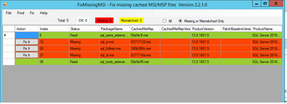
When you run the utility it will ask you for the installer drive, by default this is c:\windows\installer it may return something like this:

Hopefully it will return an empty table, however if it does return data we know what to do to fix it.

You can see that in the screen dump I’ve fixed two missing msi’s and failed to fix 3.  However this does give us really useful information.  We know what the msi we are missing relates to and the number SQL Server has given to it.  SQL Server randomizes the CachedMSIMsp so you can’t just find that one.

Instead what you have to do to fix this is search out the package name, sql_is.msi, by the time I’d got to this point  I’d downloaded the version of SQL Server I was working with and tried a repair which had failed.  Search for the package name, so looking at the first one it’s sql_is.msi, copy it to c:\windows\installer and rename it to, in our case, 83717132.msi, repeat this for all missing msi’s and then you should be able to re-run the service pack successfully.

The post Service Pack – Fix Missing MSI issue appeared first on Simple Talk.

from Simple Talk https://ift.tt/2Pd2uvP
via

Distractions at Work

Many jobs in technology, especially those that involve writing code, take concentration and focus. It’s often called being “in the zone.” For me, it feels like I’m inside a bubble where time goes at a different pace than the rest of the world. In fact, the rest of the world seems to disappear when I’m in the zone…until I’m interrupted, that is.

Studies have been done to measure how long it takes developers to become productive again after being interrupted, and 15 to 20 minutes is usually reported. One study from the University of California Irvine found it took an average of 23 minutes for managers to get back on task, but they became accustomed to interruptions and worked harder to make it up.

Distractions can come in many forms. In today’s world of open offices, it’s hard to concentrate. It’s difficult to tune out all the conversations. The worst is when a co-worker puts a conference call on speakerphone. Why do that? The idea behind these environments is that workers will collaborate more, but there is nowhere to hide when you need to be left alone to get some work done. These floorplans encourage chit-chat and “drive-by” requests, and some developers resort to headphones to tune out the noise.

Even sanctioned work tools like company email can be distractions when you are writing code or solving a performance problem. Author Tim Ferriss recommends spending just one hour per week on Monday morning to read email in his book The 4-Hour Workweek. In my opinion, that schedule is not going to work for most people in any IT role or those who don’t want to miss messages from managers. Maybe it makes sense to limit checking work email messages to twice a day if one hour a week is not frequent enough.

Many companies are limiting emails and instead are using tools like Slack to communicate among teams. The idea is that, if you are at your desk, you will immediately see the message and be expected to respond. In his article about how to eliminate distractions from Slack, author Joe Casabona says “Slack makes it very easy for people to take you out of the moment – it’s the virtual knock on the door and, ‘hey you have a minute?’” (And don’t get me started about the number of channels I’m expected to watch!)

Disruptions decrease productivity and ultimately hurt the bottom line. Maybe one day, someone will design the perfect office, and companies will implement “no interruption time” policies. Until then, it’s back to the headphones.

Commentary Competition

Enjoyed the topic? Have a relevant anecdote? Disagree with the author? Leave your two cents on this post in the comments below, and our favourite response will win a $50 Amazon gift card. The competition closes two weeks from the date of publication, and the winner will be announced in the next Simple Talk newsletter.

The post Distractions at Work appeared first on Simple Talk.

from Simple Talk https://ift.tt/2qjC3Ld
via

Building a Countdown Timer with PowerShell

When one thinks of PowerShell, one thinks of it as a scripting language. Generally, this is true. While you can write a script that prompts for input and provides output, usually there are no real GUI elements involved, and a cursory glance at the list of PowerShell cmdlets reinforces this idea.

However, it is possible to create a GUI with PowerShell; it just takes a bit more work. Furthermore, once one understands how to do this, it can lead to far more powerful scripts in the future.

A Simple Timer

As with some of my projects, this one started as sort of a challenge to myself. I wanted to create a script that created a form on the screen, and I wanted it to do something. I decided to start with something simple, a form that counted down the time and then closed. (NOTE: The examples in this article work in classic PowerShell but not PowerShell Core since Core is multiplatform.)

Save the following script as Countdown Timer_1.ps1.

$delay = 10
$Counter_Form = New-Object System.Windows.Forms.Form
$Counter_Form.Text = "Countdown Timer!"
$Counter_Form.Width = 450
$Counter_Form.Height = 200
$Counter_Label = New-Object System.Windows.Forms.Label
$Counter_Label.AutoSize = $true 
$Counter_Form.Controls.Add($Counter_Label)
while ($delay -ge 0)
{
  $Counter_Form.Show()
  $Counter_Label.Text = "Seconds Remaining: $($delay)"
  start-sleep 1
  $delay -= 1
}
$Counter_Form.Close()

The loop should be self-evident. It starts with the selected $delay value and counts down, sleeping for 1 second at a time until it hits 0. Note that due to how PowerShell works, the one-second delay in start-sleep has some slop to it. You should not use this script to launch a space shuttle, but for everyday use it’s fine.

The interesting part of this script is not the loop; it’s the New-Object System.Windows.Forms.Form line. To anyone who has worked with C# or VB.Net or any other .Net managed code, this should look familiar. You are simply calling into the .Net Framework to create a form. This innocuous statement will mean huge ramifications later.

Once you have your form object, you can start to assign some properties, in this case, the title (in the .text) property and height and width.

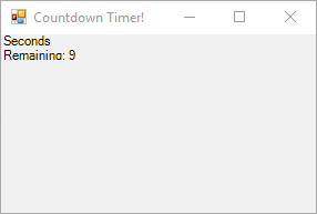
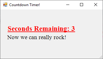
Finally, you need to put a new object on this form, a label. Once you’ve done that, you simply loop through for the length of your $delay and the form will count down. You should see a screen that looks like this. (Note that the scripts in this article were tested on Dell and Lenovo laptops, an old HP desktop, and an Azure VM but no guarantee that the forms will look the same on all machines. You may have to tweak some of the numbers in the scripts to see the same results.)

It’s not pretty, but it gets the job done. To fix some of the more obvious problems and create something a bit nicer looking, save the following script as Coutndown Timer_2.ps1.

$delay = 10
$Counter_Form = New-Object System.Windows.Forms.Form
$Counter_Form.Text = "Countdown Timer!"
$Counter_Form.Width = 450
$Counter_Form.Height = 200
$Counter_Label = New-Object System.Windows.Forms.Label
$Counter_Label.AutoSize = $true
$Counter_Label.ForeColor = "Green"
$normalfont = New-Object System.Drawing.Font("Times New Roman",14)
$Counter_Label.Font = $normalfont
$Counter_Label.Left = 20
$Counter_Label.Top = 20
$Counter_Form.Controls.Add($Counter_Label)
while ($delay -ge 0)
{
  $Counter_Form.Show()
  $Counter_Label.Text = "Seconds Remaining: $($delay)"
  if ($delay -lt 5)
  { 
     $Counter_Label.ForeColor = "Red"
     $fontsize = 20-$delay
     $warningfont = New-Object System.Drawing.Font("Times New Roman",$fontsize,[System.Drawing.FontStyle]([System.Drawing.FontStyle]::Bold -bor [System.Drawing.FontStyle]::Underline))
     $Counter_Label.Font = $warningfont
  } 
 start-sleep 1
 $delay -= 1
}
$Counter_Form.Close()

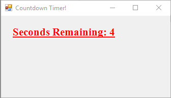
You should get something like this when you run the script:

 

You now have a countdown timer that you can control the label position, font size, style and color which is all very useful. In this case, I took advantage of the ability to move the label down a bit, make the font larger and to change color and size as the countdown approached 0.

Adding Functionality

The previous example is a simple timer, but to make it useful, you will need to add some controls. Again, you can take advantage of the fact that classic PowerShell can make calls into the Windows forms dll.

In addition, you will take advantage of the ability to pass parameters as you start to make this a fully functional application. This time, you will add a new label, a text edit box and OK and Cancel buttons. Combined, all these should give you a fully functional countdown timer.

The following script combines all of the above:

param([int]$delay=3, [string]$EventLabel = "This is a test")
#Setup initial form
$Counter_Form = New-Object System.Windows.Forms.Form
$Counter_Form.Text = "Countdown Timer!"
$Counter_Form.Width = 450
$Counter_Form.Height = 200
$Counter_Form.WindowState = "Normal"
#Setup our Normal font
$normalfont = New-Object System.Drawing.Font("Times New Roman",14)
#Setup initial label
$Counter_Label = New-Object System.Windows.Forms.Label
$Counter_Label.AutoSize = $true
$Counter_Label.ForeColor = "Green"
$Counter_Label.Font = $normalfont
$Counter_Label.Left = 20
$Counter_Label.Top = 50
#setup input areas
$Counter_GetDelay_Label = New-Object System.Windows.Forms.Label
$Counter_GetDelay_Label.AutoSize = $true
$Counter_GetDelay_Label.Text = "Enter Delay:"
$Counter_GetDelay_Label.Left = 10
$Counter_GetDelay_Label.Top = 8
$Counter_Form.Controls.Add($Counter_GetDelay_Label)
$Counter_GetDelay_TextBox = New-Object System.Windows.Forms.TextBox
$Counter_GetDelay_TextBox.AutoSize = $true 
$Counter_GetDelay_TextBox.Text = $delay
$Counter_GetDelay_TextBox.Left = $Counter_GetDelay_Label.Left + $Counter_GetDelay_Label.Width + 10
$Counter_GetDelay_TextBox.Top = 5
$Counter_Form.Controls.Add($Counter_GetDelay_TextBox)
$Counter_Event_Label = New-Object System.Windows.Forms.Label
$Counter_Event_Label.AutoSize = $true 
$Counter_Event_Label.Text = $EventLabel
$Counter_Event_Label.Location = '20,100' # note we're using a different method to position the text here.
$Counter_Event_Label.Font = $normalfont
#Setup and handle the OK button
$Counter_OKButton = New-Object System.Windows.Forms.Button
$Counter_OKButton.AutoSize = $true 
$Counter_OKButton.Text = "Ok"
$Counter_OKButton.Left = 80
$Counter_OKButton.Top = 40
$Counter_OKButton.Add_Click({
  $delay=$Counter_GetDelay_TextBox.Text
  $Counter_Form.Controls.Remove($Counter_GetDelay_Label)
  $Counter_Form.Controls.Remove($Counter_GetDelay_TextBox)
  $Counter_Form.Controls.Remove($Counter_OKButton)
  $Counter_Form.Controls.Remove($Counter_CancelButton)
  $Counter_Form.Controls.Add($Counter_Label)
  $Counter_Form.Controls.Add($Counter_Event_Label)
  while ($delay -gt 0)
  {
      $Counter_Label.Text = "Seconds Remaining: $($delay)"
      if ($delay -lt 5)
      { 
          $Counter_Label.ForeColor = "Red"
          $fontsize = 20-$delay
          $warningfont = New-Object System.Drawing.Font("Times New Roman",$fontsize,[System.Drawing.FontStyle]([System.Drawing.FontStyle]::Bold -bor [System.Drawing.FontStyle]::Underline))
          $Counter_Label.Font = $warningfont
      } 
      start-sleep 1
      $delay -= 1
   }
   $Counter_Form.Close()
  }
)
$Counter_Form.Controls.Add($Counter_OKButton)
#Setup and handle the cancel button
$Counter_CancelButton = New-Object System.Windows.Forms.Button
$Counter_CancelButton.AutoSize = $true 
$Counter_CancelButton.Text = "Cancel"
$Counter_CancelButton.Left = $Counter_OKButton.Left + $Counter_OKButton.Width + 10
$Counter_CancelButton.Top = 40
$Counter_CancelButton.Add_Click({$counter_form.Close() })
$Counter_Form.Controls.Add($Counter_CancelButton)
#Setup and handle keyboard Enter/Escape
$Counter_Form.AcceptButton=$Counter_OKButton
$Counter_Form.CancelButton=$Counter_CancelButton
#Finally, we show the dialog
$Counter_Form.ShowDialog() | Out-Null #absorbs cancel message at end. This occurs for reasons outside scope of this article

You can call it from the command line and pass the parameter –EventLabel “Now we can really rock!”

& '.\Countdown Timer_3.ps1' -EventLabel "Now we can really rock!"

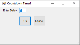
When you run it, you will get something like this:

Clicking the Ok button will result in the following:

I will leave it to you as the reader to figure out how to add the possibility of editing the passed in EventLabel parameter within the dialog box.

Controlling the Form Position

When you run this multiple times, you will notice that the position of the dialog box itself changes each time. The next version will fix this. In fact, in the next step, you will make this a fairly functional countdown timer that fills up most of the screen and looks professional.

param([int]$delay=3, [string]$EventLabel = "This is a test")
#Get monitor resolution of primary monitor
$monitordetails = [System.Windows.Forms.SystemInformation]::PrimaryMonitorSize
$monitorheight = $monitordetails.Height
$monitorwidth = $monitordetails.Width
#Setup initial form
$Counter_Form = New-Object System.Windows.Forms.Form
$Counter_Form.Text = "Countdown Timer!"
$Counter_Form.Height = $monitorheight * .80
$Counter_Form.Width = $monitorwidth * .80
$Counter_Form.WindowState = "Normal"
$Counter_Form.Top = $monitorheight *.10
$Counter_Form.Left = $monitorwidth *.10
$Counter_Form.StartPosition = "manual"     # this ensures we can control where on the screen the form appears
#Setup our Normal font
$normalfont = New-Object System.Drawing.Font("Times New Roman",28)   # We will use this size and type of font throughout
#Setup initial label
$Counter_Label = New-Object System.Windows.Forms.Label
$Counter_Label.ForeColor = "Green"
$Counter_Label.Font = $normalfont
#setup input areas
# This will let prompt for the delay if it wasn't passed in on the command line.
$Counter_GetDelay_Label = New-Object System.Windows.Forms.Label
$Counter_GetDelay_Label.AutoSize = $true
$Counter_GetDelay_Label.Text = "Enter Delay:"
$Counter_GetDelay_Label.Left = 10
$Counter_GetDelay_Label.Top = 8
$Counter_Form.Controls.Add($Counter_GetDelay_Label)
$Counter_GetDelay_TextBox = New-Object System.Windows.Forms.TextBox
$Counter_GetDelay_TextBox.AutoSize = $true 
$Counter_GetDelay_TextBox.Text = $delay
$Counter_GetDelay_TextBox.Left = $Counter_GetDelay_Label.Left + $Counter_GetDelay_Label.Width + 10
$Counter_GetDelay_TextBox.Top = 5
$Counter_Form.Controls.Add($Counter_GetDelay_TextBox)
$EventLabel_Size= [System.Windows.Forms.TextRenderer]::MeasureText($EventLabel, $normalfont)
$Counter_Event_Label = New-Object System.Windows.Forms.Label
$Counter_Event_Label.Width = $EventLabel_Size.Width+6  # Apparently despite giving it the string, we need a little extra room.
$Counter_Event_Label.Height= $EventLabel_Size.Height
$Counter_Event_Label.Text = $EventLabel
$Counter_Event_Label.Left = ($Counter_Form.Width/2)-($EventLabel_Size.Width/2)
$Counter_Event_Label.Top = ($Counter_Form.Height/2)-($EventLabel_Size.Height/2)
$Counter_Event_Label.Font = $normalfont
#Setup and handle the OK button
$Counter_OKButton = New-Object System.Windows.Forms.Button
$Counter_OKButton.AutoSize = $true 
$Counter_OKButton.Text = "Ok"
$Counter_OKButton.Left = 80
$Counter_OKButton.Top = 40
$Counter_OKButton.Add_Click({
   # Get our delay the user entered.
   $delay=$Counter_GetDelay_TextBox.Text
  
   # Get rid of the controls we don't need any more.
   $Counter_Form.Controls.Remove($Counter_GetDelay_Label)
   $Counter_Form.Controls.Remove($Counter_GetDelay_TextBox)
   $Counter_Form.Controls.Remove($Counter_OKButton)
   $Counter_Form.Controls.Remove($Counter_CancelButton)
   # Now add the labels we want.
   $Counter_Form.Controls.Add($Counter_Label)
   $Counter_Form.Controls.Add($Counter_Event_Label)
   while ($delay -gt 0)
   {
      $Counter_Label.Text = "Seconds Remaining: $($delay)"
      $Counter_LabelSize= [System.Windows.Forms.TextRenderer]::MeasureText($Counter_Label.Text , $normalfont) # we need this so we can figure where to put the countdown labeled, centered.
      $Counter_Label.Font = $normalfont
      $Counter_Label.AutoSize = $true
      $Counter_Label.Left = ($Counter_Form.Width/2)-($Counter_LabelSize.Width/2)  # We want it centered.
      $Counter_Label.Top = $Counter_Form.Height * .3 # We want it near the bottom of the screen.
      if ($delay -le 5)  # Now things are getting close, let's change the color and make it bolder and underline it
      { 
          $Counter_Label.ForeColor = "Red"
          $warningfont = New-Object System.Drawing.Font("Times New Roman",28,[System.Drawing.FontStyle]([System.Drawing.FontStyle]::Bold -bor [System.Drawing.FontStyle]::Underline))
          $Counter_Label.Font = $warningfont
          $Counter_LabelSize= [System.Windows.Forms.TextRenderer]::MeasureText($Counter_Label.Text , $warningfont)
          $Counter_Label.Width = $Counter_LabelSize.Width + 10
          $Counter_Label.Left = ($Counter_Form.Width/2)-($Counter_LabelSize.Width/2)
      } 
      start-sleep 1
      $delay -= 1
  }
  $Counter_Form.Close()
})
$Counter_Form.Controls.Add($Counter_OKButton)
#Setup and handle the cancel button
$Counter_CancelButton = New-Object System.Windows.Forms.Button
$Counter_CancelButton.AutoSize = $true
$Counter_CancelButton.Text = "Cancel"
$Counter_CancelButton.Left = $Counter_OKButton.Left + $Counter_OKButton.Width + 10
$Counter_CancelButton.Top = 40
$Counter_CancelButton.Add_Click({$counter_form.Close() })
$Counter_Form.Controls.Add($Counter_CancelButton)
#Setup and handle keyboard Enter/Escape
$Counter_Form.AcceptButton=$Counter_OKButton
$Counter_Form.CancelButton=$Counter_CancelButton
#Finally, we show the dialog
$Counter_Form.ShowDialog() | Out-Null #absorbs cancel message at end. This occurs for reasons outside scope of this article

You’ve now created a fully functional countdown timer that will automatically scale to the size of the screen and allow you to configure how long it runs for and what primary message it displays. Future improvements might be to allow the option of having a background graphic and being able to more easily abort the timer in the middle of it running.

Conclusion

Hopefully, now you can see that through the power of PowerShell, in combination with the built-in .Net capabilities, you can create full-fledged applications that can interact with the user, prompting them for input and also providing them with output. In fact, pretty much anything you can do in C# or VB.Net can be done in a very similar fashion in PowerShell without needing to write a full-blown application. That said, writing an application like this using PowerShell ISE can be tedious. For example, it took me a while to get the positioning correct, mostly due to a few typos here and there (for example, using width when I meant height and vice versa). There are plug-ins for Visual Studio and other stand-alone IDEs that can make this task easier. But I wanted to demonstrate the power of PowerShell out of the box without any further add-ons or tools.

All scripts in this article are also available at: https://github.com/stridergdm/SimpleTalk_PowerShell-Scripts

 

The post Building a Countdown Timer with PowerShell appeared first on Simple Talk.

from Simple Talk https://ift.tt/34WAW3r
via

The Gloop: An Easier way of Managing SQL Server Documentation

Here, in this blog, I’m continuing a theme that I started in a previous blog, ‘What’s in that database? Getting information about routines’.

In that blog, I just wanted to provide a few examples of extracting metadata from SQL Server into Powershell and hinting about why one might want to do it. I’ll now show how to save the details of the metadata of your database, including tables and routines, in JSON files. Then I’ll demonstrate how to change and add to the descriptions of database objects and saving them to the database.

Metadata extract files are handy for documentation, study, cataloguing and change-tracking. This type of file supplements source because it can record configuration, permissions, dependencies and documentation much more clearly. It is a good way of making a start with documenting your database.

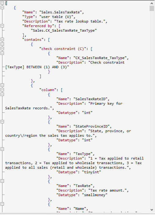
Here is a sample of a json metadata file (from AdventureWorks 2016). It was generated using GloopCollectionOfObjects.sql that is here in Github, and is being viewed in JSONBuddy. I use this format of JSON, a collection of documents representing SQL Server base objects (no parent objects) when I need to read the contents into MongoDB. The term ‘Gloop’ refers to a large query that, you’d have thought, would be better off as a procedure. Here is a typical sample of the output.

Ok. Those descriptions make a huge difference to readability. I want to be able to edit them in JSON and save them back to the database. OK. We can do that. I use #ParseJSONMetadataToUpdateTheDocumentation which is in the GitHub folder. It is a temporary stored procedure. We can either use this from a SQL batch or call it in SQL using PowerShell.

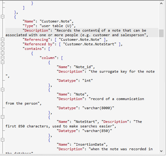
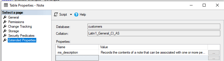
Without wishing to change our AdventureWorks file, We’ll open up a sample file called ‘Customers’ and add some descriptions. In this next screendump, I’m adding a description to a table called Customer.note

Then we save the file and execute this code.

USE customers
DECLARE @JSON NVARCHAR(MAX);
SELECT @JSON = BulkColumn
  FROM
  OpenRowset(BULK 'PathToTheData\customers.json', SINGLE_NCLOB)
  AS MyJSONFile;
DECLARE @howManyChanges INT;
EXECUTE #ParseJSONMetadataToUpdateTheDocumentation @JSON, @howManyChanges OUTPUT;
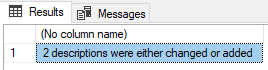
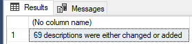
SELECT Convert(VARCHAR(5),@howManyChanges)+ ' descriptions were either changed or added'

 

Why 2? I added a description to a column as well.

… and we can check to make sure that the right thing got changed.

If we delete all the extended properties and then re-run the batch we get this

Phew, they are all back in there.

What’s the best way to execute and write out the SQL Gloop query to get the metadata extract in the first place? It can be done in SQL, but once you’ve decided that you need to work on a whole collection of servers and their databases, or you have a regular database chore to do that involves saving to files, it is worth considering doing the chore in SQL, but using a PowerShell task that can be scheduled. I’ve included the code for this on Github called RunSQLScript.ps1

In my previous Blog, I introduced the idea of getting metadata about your database using SQL, and saving the contents into a directory, but I didn’t really go into the details about how you run such code. I also mentioned that, if you are running the same task on a number of databases, there is no shame attached to running a large query to extract the metadata from your databases. I referred to this as a ‘Gloop’. The reason for doing so is that you can run it on a number of databases but leave no trace of utility procedures on them, not even a temporary stored procedure. GloopCollectionOfObjects.sql is one of these and I’ve added others to the Github site that were written for other purposes.

Developing other uses for Metadata extracts

There are several good uses for metadata extracts of database objects and their associated columns, indexes, parameters and return values. The main reason I have for wanting to do this is to see what’s been properly documented in the database and where something is missing, adding it. There are plenty of other uses. What you collect depends on the nature and purpose of your task. I’ve added some sample Gloop queries to deliver different formats of JSON files. Beware, though, that you can’t save the documentation without altering the SQL code in the temporary procedure that shreds it into a relational table.

Whatever use that one puts these metadata extracts to, one thing always happens: When you are looking at metadata in another format than the build script, then some things, mostly mistakes and omissions, that you have just never noticed before will now stick out clearly. It seems to help to get a different view of your database.

We must also decide on the format we want for our data. If we are predominately using it for documentation, then readability is important. For doing comparisons or keeping a record of database changes in source control, maybe you want something that can be read by input routines more easily. Although ordered arrays are legal JSON, they aren’t easy to produce in SQL Server because SQL Server’s JSON library is geared to produce key/value pairs. Tables have names that translate easily to keys since the schema/name combination is unique. The same is true of columns and parameters. The natural way of recording these might be to have an array of schemas, each of which have arrays of table objects using their name as a key. However, they are ordered arrays of objects. It isn’t a major difficulty because we can do what SQL Server does, and put the name as a value assigned to a ‘name’ key. It just looks clunky if you are reading the JSON. However, it makes it easier to query in MongoDB, and to read into relational table format.

Editing JSON-based metadata With Studio3T

With Studio3T, you can just import each file as a collection into a database. I use a MongoDB database Called SQLServerMetadata, and import each database as a collection under its SQL Server name. This provides me with a separate collection for each database, with a document representing a base object such as a Function, Table, Procedure or View. This allows me to edit each object individually and save it back to the collection. Then I can export it back out.

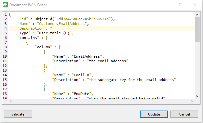
Here, I’m just beginning to document the table itself. I can edit the documentation for each table individually because each base object (Function, Table, Procedure, Rule, View or Default) is a document in MongoDB terms and I can, with Studio3T, edit each document separately and have it checked instantly as I save the edits. This means I can even edit the documentation for procedures and functions, their parameters and columns (table-valued functions and views have them- it is helpful to your team members to document them)

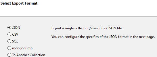
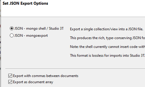
Having made my changes, I then save them back to the file. I do it via Studio3T’s collection-export facilities. I use

… and on the next page in the wizard …

I can even paste individual documents from Studio3T into SQL and see that I’ve made all the necessary changes. Unfortunately, MongoDB inserts surrogate primary keys in a form of ‘extended JSON’ that isn’t compatible. You need to nick them out. To do this you can use a Regex. In a file, or in SSMS, use …
‘”_id”.+’
…as the regex expression (without the single bracket delimiters!), and a blank replacement text

You can then inspect the results using the SQL that that is used within the ParseJSONMetadataToUpdateTheDocumentation.sql on Github.

DECLARE @JSON NVARCHAR(MAX);
SELECT @JSON = BulkColumn
  FROM
  OpenRowset(BULK 'PathToTheData\customers.json', SINGLE_NCLOB)
  AS MyJSONFile;

DROP TABLE IF EXISTS #TheObjects;
CREATE TABLE #TheObjects
  (
  Name sysname NOT NULL,
  Type NVARCHAR(30) NOT NULL,
  Description NVARCHAR(3750) NULL,
  ParentName sysname NULL,
  [Contains] NVARCHAR(MAX) NULL
  );

INSERT INTO #TheObjects (Name, Type, Description, ParentName, [Contains])
  SELECT BaseObjects.Name, BaseObjects.Type, BaseObjects.Description, NULL,
    [Contains]
    FROM
    OpenJson(@JSON)
    WITH
      (
      Name NVARCHAR(80) '$.Name', Type NVARCHAR(80) '$.Type',
      Parent NVARCHAR(80) '$.Parent',
      Description NVARCHAR(MAX) '$.Description',
      [Contains] NVARCHAR(MAX) '$.contains' AS JSON
      ) AS BaseObjects;

INSERT INTO #TheObjects (Name, Type, Description, ParentName, [Contains])
  SELECT objvalues.Name, obj.[Key] AS Type, objvalues.Description,
    #TheObjects.Name AS ParentName, NULL AS [contains]
    FROM #TheObjects
      OUTER APPLY OpenJson(#TheObjects.[Contains]) AS child
      OUTER APPLY OpenJson(child.Value) AS obj
      OUTER APPLY
    OpenJson(obj.Value)
    WITH (Name NVARCHAR(80) '$.Name', Description NVARCHAR(MAX) '$.Description') AS objvalues;


DROP TABLE IF EXISTS #EPParentObjects;
CREATE TABLE #EPParentObjects
  (
  TheOneToDo INT IDENTITY(1, 1),
  level0_type VARCHAR(128) NULL,
  level0_Name sysname NULL,
  level1_type VARCHAR(128) NULL,
  level1_Name sysname NULL,
  level2_type VARCHAR(128) NULL,
  level2_Name sysname NULL,
  [Description] NVARCHAR(3750),
  );

INSERT INTO #EPParentObjects
  (level0_type, level0_Name, level1_type, level1_Name, level2_type,
level2_Name, Description)
  SELECT 'schema' AS level0_type, ParseName(Name, 2) AS level0_Name,
      CASE WHEN Type LIKE '%FUNCTION%' THEN 'FUNCTION'
        WHEN Type LIKE '%TABLE%' THEN 'TABLE'
        WHEN Type LIKE '%PROCEDURE%' THEN 'PROCEDURE'
        WHEN Type LIKE '%RULE%' THEN 'RULE'
        WHEN Type LIKE '%VIEW%' THEN 'VIEW'
        WHEN Type LIKE '%DEFAULT%' THEN 'DEFAULT'
        WHEN Type LIKE '%AGGREGATE%' THEN 'AGGREGATE'
        WHEN Type LIKE '%LOGICAL FILE NAME%' THEN 'LOGICAL FILE NAME'
        WHEN Type LIKE '%QUEUE%' THEN 'QUEUE'
        WHEN Type LIKE '%RULE%' THEN 'RULE'
        WHEN Type LIKE '%SYNONYM%' THEN 'SYNONYM'
        WHEN Type LIKE '%TYPE%' THEN 'TYPE'
        WHEN Type LIKE '%XML SCHEMA COLLECTION%' THEN 'XML SCHEMA COLLECTION' 
            ELSE'UNKNOWN' 
          END AS level1_type,
    ParseName(Name, 1) AS level1_Name, NULL AS level2_type,
    NULL AS level2_Name, Description
    FROM #TheObjects
    WHERE ParentName IS NULL;

INSERT INTO #EPParentObjects
  (level0_type, level0_Name, level1_type, level1_Name, level2_type,
level2_Name, Description)
  SELECT level0_type, level0_Name, level1_type, level1_Name,
      CASE WHEN Type LIKE '%COLUMN%' THEN 'COLUMN'
        WHEN Type LIKE '%CONSTRAINT%' THEN 'CONSTRAINT'
        WHEN Type LIKE '%EVENT NOTIFICATION%' THEN 'EVENT NOTIFICATION'
        WHEN Type LIKE '%INDEX%' THEN 'INDEX'
        WHEN Type LIKE '%PARAMETER%' THEN 'PARAMETER'
        WHEN Type LIKE '%TRIGGER%' THEN 'TRIGGER' 
                ELSE 'UNKNOWN' 
          END AS Level2_type,
    #TheObjects.Name AS Level2_name, #TheObjects.Description
    FROM #EPParentObjects
      INNER JOIN #TheObjects
        ON level1_Name = ParseName(ParentName, 1) 
                  AND level0_Name =ParseName(ParentName, 2);

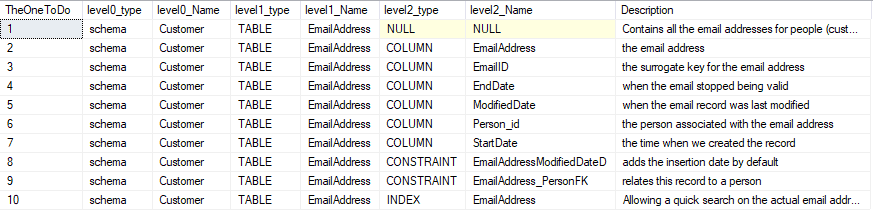
SELECT * FROM #EPParentObjects AS EPO

 

If you think that this table looks suspiciously like the parameters you’d need to use for the various SQL system procedures that you’d need to use, you’re right. That is the underlying purpose of the code!

Hmm. Looks good.

Studio3T has the option of putting the resulting JSON for a database on the clipboard so you can even do the job without having to think of a way of reading the JSON into SQL Server. However, I’ve already demonstrated an easy way of doing that.

Conclusions

This is an approach to documentation that suits me fine. If you know of a better way, let me know! There are a number of different ways that you can do this, so all you need to do is to edit the Gloop to be closer to what you need. Make sure that, if you change the structure of the JSON produced by the Gloop, you make the equivalent changes to the SQL that shreds the JSON into a relational format for updating your documentation.

Just as a thought. If you put the JSON for your documentation in source control, you can then use it for inserting the documentation into a database build. It is a lot easier than the conventional way. It means that, if you keep it up to date, it also allows you to track the changes in the database even if you are using a migrations-scripts-first approach.

 

The post The Gloop: An Easier way of Managing SQL Server Documentation appeared first on Simple Talk.

from Simple Talk https://ift.tt/2rPLG4L
via

Storage 101: Welcome to the Wonderful World of Storage

The series so far:

• Storage 101: Welcome to the Wonderful World of Storage

Gone are the days when implementing storage was simply a matter of standing up a few disk drives. Today’s data-intensive workloads require a variety of storage solutions to handle the unprecedented amounts of heterogeneous data. At the same time, storage technologies are quickly evolving, with new options available every day. Administrators can now choose from a wide range of storage types and configurations. Unfortunately, it’s not always clear which ones might best meet their needs.

This article is the first in a series that examines the diverse world of today’s storage solutions. In this series, I plan to cover everything from storage fundamentals, such as device types and storage metrics, to more advanced topics, ranging from hyperconvergence to intelligent storage. The goal is to provide you with a foundation for better understanding of current storage technologies and how to use them in your organization to support your data-intensive workloads. This article provides a starting point toward that goal by introducing you to basic concepts that serve as building blocks for today’s storage solutions.

Storage Media

Two types of storage media support most of today’s application workloads: hard-disk drives (HDDs) and solid-state drives (SSDs). Both are forms of non-volatile storage. In other words, they can persist data even if the power gives out, unlike traditional random-access memory (RAM), which is much faster, but also costlier and, of course, volatile.

The HDD has long had the reputation as the data center’s go-to workhorse for supporting an assortment of applications. Over the years, it has steadily evolved to handle greater volumes of data while delivering better read and write performance.

The HDD contains one or more spinning platters on which the data is stored. The platters are protected within sealed casing, along with other components, such as the magnetic heads that read the data. Today’s HDDs can store 16 TB or more of data and, despite the wave of SSDs, continue to play a vital role in enterprise storage.

Even so, the SSD has made significant inroads into data centers of all sizes, in part because of increased demand for high-performing storage, but also because of technological improvements and plummeting prices.

Unlike the HDD, the SSD includes no moving parts and instead stores data on interconnected silicon chips, resulting in better performance, while requiring less space and power. Currently, most SSD storage is based on NAND flash technologies, in which data bits are stored in cells and regulated with electric charges.

Both HDDs and SSDs come with advantages and disadvantages (a discussion I’ll save for later in the series). For this reason, many organizations opt to use both, employing SSDs for high-performing workloads and sticking with HDDs for the rest.

Some organizations have also implemented hybrid arrays, storage systems that incorporate both HDDs and SSDs. The exact ratio of HDDs to SSDs, as well as the array’s configuration, depends on the hybrid solution itself, but the result is the same. You get the benefits of both storage types while minimizing their disadvantages.

Tape storage is also still in use in some organizations, mostly for backup and archiving purposes. In a tape storage system, the data is saved to magnetic tape, which is usually encased in some type of cassette or cartridge. Tape storage is not particularly fast or efficient, in terms of supporting data-intensive workloads, but it can store large quantities of data at a relatively low price when compared to the other storage options.

Interfaces, Form Factors, and Storage Protocols

When it comes to storage, few topics cause as much confusion as the terms interface, form factor, and storage protocol. Throughout the industry, these terms are used interchangeably, inconsistently, and imprecisely when describing storage-related technologies. As it turns out, there’s a good reason for this. Many of these technologies don’t fit neatly into any one of these categories or into other categories for that matter, which makes it possible to describe them in multiple ways.

For example, Serial Advanced Technology Attachment (SATA) is commonly referred to as a connection interface. SATA is one of the most popular interfaces out there, supporting a wide variety of HDD and SSD storage devices. Compared to its predecessor—Parallel Advanced Technology Attachment (PATA)—SATA is faster, requires smaller physical connectors, and supports hot-swapping capabilities.

In addition to being referred to as an interface, SATA is also referred to as a form factor and a protocol. This is because SATA is as much a standard as it is an interface and, as such, defines a complete methodology for connecting storage devices to computer systems and for transferring data. As a result, the term SATA is often used to reference components throughout the storage stack, including the transport layer, physical connectors and storage devices themselves.

To help bring order to this muddle, at least for the purposes of this series, I use the term interface to refer specifically to how a storage device connects to a computer. The interface defines the physical and logical characteristics for enabling data transfers, which can include everything from the computer’s bus connectors to the signaling technology that drives data transfers.

Related to the interface is the form factor, which refers the size and shape of the storage device, and the protocol, which is a set of rules that define how the storage device and computer communicate with each other. A storage device of a specific form factor connects to the computer via an interface, using a protocol to determine how to pass data to and from the computer.

Let’s look at an example to help clarify how all this works. Another technology that qualifies as an interface is Peripheral Component Internet Express (PCIe), which, unlike other interfaces, makes it possible to connect a storage device directly to the motherboard. Because of this direct connection, PCIe can boost performance and reduce latencies. In addition, PCIe expansion slots come in multiple configurations, which are based on the number of data lanes. For example, an x16 expansion slot uses 16 data lanes.

The PCIe interface has been around for several years, primarily supporting peripheral devices such as graphic or network cards. More recently the PCIe interface has found a home with the SSD, which can take better advantage of the faster data transfer speeds than the typical HDD, especially with the introduction of the Non-Volatile Memory Express (NVMe) protocol.

NVMe is a relatively new protocol developed from the ground up to accommodate the needs of PCIe-connected SSD storage devices. The protocol leverages parallel, low-latency data paths to enable high-performing transfers.

At the same time, NVMe is more than just a protocol. It’s a communication standard that defines multiple components, including a register interface and command set, as well as a management interface. Even so, NVMe is commonly referred to as a storage protocol, although I’ve also seen it referred to as an interface and form factor. (Confused yet?)

In recent years, the PCIe/NVMe duo has become extremely popular. The storage market is now flush with SSD products that fit into PCIe slots and use the NVMe protocol to transfer data. And because PCIe supports multiple expansion slots, the SSDs are available in a variety of form factors.

For example, many vendors now offer SSDs in the M.2 form factor, which comes in a variety of sizes, such as 22mm X 30 mm, 22mm X 80mm, or 30mm X 42mm. What makes the M.2 form factor even more unique is that it’s available for both the SATA interface and the PCIe interface. A PCIe-based SSD with an M.2 form factor is essentially a PCIe card that fits into a PCIe slot. The SSD uses the PCIe interface to connect to the computer and uses the NVMe protocol to carry out communications and transfer data.

Not surprisingly, the topic of interfaces, form factors, and storage protocols is far more involved than what I’ve covered here. Later in this series, I’ll dig into these technologies in more depth. But for now, let’s move on to storage configurations.

Storage Configurations

For the purposes of this article, when I talk about storage configurations, I’m referring primarily to direct-attached storage (DAS), network-attached storage (NAS), and the storage area network (SAN), with cloud storage thrown into the mix to shake things up.

As the name suggests, DAS refers to storage devices that attach directly to a computer through one of the common interfaces, such as SATA, PCIe, USB, or Thunderbolt. DAS is the most basic of the three configurations and does not support many of the advanced features available to the other configurations. At the same time, DAS is usually the easiest to implement and maintain and the least expensive. However, DAS is not particularly scalable, which tends to limit its use to small-business setups that share data locally.

In general, DAS has had a diminishing role in supporting many of today’s more robust applications. However, the emergence of the hyperconverged infrastructure (HCI) has breathed new life into DAS. Most HCI platforms are made up of multiple server nodes, each with its own storage. The storage is abstracted across all nodes to create logical resource pools available to applications running in the HCI environment.

For many workloads, IT teams are more inclined to implement a NAS (network-attached storage) solution, which is commonly deployed as an array of storage devices connected through the local area network (LAN). The solution has its own processing and memory resources, along with its own operating system (OS) and supporting software. Compared to DAS, a NAS solution is more scalable, and it supports more advanced features, such as thin provisioning and snapshots. But it’s also more expensive.

Next up the ranks is the SAN (storage area network), a high-performing storage solution typically used in larger data centers to support enterprise workloads and mission-critical applications. A SAN often runs in a dedicated network such as Fibre Channel. It is more complex and expensive than the other options, but also more scalable, resilient, and performant, with consistently high throughputs and low latencies. A SAN offers the best of both DAS and NAS solutions, but at a price.

Although NAS and SAN systems have served as the backbone for most enterprise applications, many organizations are now turning to the cloud to meet their storage needs. Cloud vendors provide on-demand storage services with pay-as-you-go subscription models, helping to avoid over-provisioning and extensive up-front costs.

Cloud platforms are highly scalable, easy to manage, provide metered resources, and include built-in redundancy, but they can get quite pricey as subscription fees add up. In addition, they don’t offer the level of control you get with on-premises storage.

To address the control issue, many organizations are turning to hybrid cloud storage, in which some data is stored on-premises and other data stored in the cloud, making it easier to ensure security, privacy, and compliance where needed. An effective hybrid solution also includes mechanisms for seamlessly managing and moving data between platforms.

Storage Types

Most storage falls into one of three categories: file, block, or object. File storage is the most basic of the three. It is the type of storage you use when you sit down at your computer and open files, save new files to disk, or inadvertently delete them. The files are stored in a hierarchical format, according to the familiar directly/subdirectory structure. Each file is tagged with a limited amount of fixed metadata, such as its name, file size, or modified date.

File storage is easy to work with and well understood by most PC users and applications, which is why it’s commonly used in DAS and NAS storage solutions. Unfortunately, file storage can get fairly cumbersome as the number of files grows, making it more difficult to scale data resources or find files when you need them.

Block storage addresses these challenges by breaking the data into chunks (blocks) and storing them as individual pieces, with no attached metadata except for a unique identifier. (Some would even argue that the identifier doesn’t qualify as metadata.) With block storage, it’s up to the managing application to determine how to organize and retrieve the blocks, keeping the data structure itself as simple as possible.

Block storage is the format of choice in a SAN storage system. Because of the lack of metadata, block storage comes with little overhead, resulting in faster data retrievals and more efficient data storage. Block storage is well suited for workloads such as relational databases, virtual desktop infrastructures, and email servers, as well as for implementing RAID arrays. On the other hand, block storage also comes with several disadvantages, such as limited scalability and increased complexity. It can also get quite pricey.

A relative newcomer to the storage scene, object storage was developed to address the growing silos of unstructured data arriving with every wave of new Internet technology—from social media to big data analytics to the Internet of Things (IoT). In object storage, data is broken into self-contained, modular units (objects) that include identifiers and customizable metadata.

Object storage has its origins in the cloud, although on-premises solutions are quickly making their mark. Because object storage is fast, flexible, and accommodates configurable metadata, it is well suited for large volumes of unstructured data, advanced analytics, and web applications, as well as for backups and archiving. But object storage is not known for its performance, and even read operations can experience latency issues. Plus, all that metadata can translate to extra overhead, impacting performance even more.

The New Age of Storage

Clearly, there are many factors to consider when planning storage for your application workloads, and the topics I’ve discussed here barely scratch the surface. As the series progresses, I’ll dig deeper into these issues and go into other aspects of storage as well to help provide a fuller picture of today’s storage landscape.

Keep in mind, however, that the storage industry is a dynamic one, with new innovations every day, driven in no small part by the steady influx of data, which is outpacing our ability to maintain it. More than ever, developers, administrators, and anyone else working with data need to understand the storage technologies at hand and the new innovations heading their way and how they might help support their data-intensive workloads now and in the foreseeable future.

 

The post Storage 101: Welcome to the Wonderful World of Storage appeared first on Simple Talk.

from Simple Talk https://ift.tt/2Ya1XO8
via

Do You Have REFERENCES?

The late Jim Gray once said that in the early days of SQL, “We had no idea what we were doing!” However, that is not completely true. What we were doing was mimicking the technologies that had gone before. The first SQL engines put each table in a separate physical file. We had file systems that had been in use for decades. We had lots of code for handling those files, in particular, all kinds of variations on index sequential access methods (ISAM). But data modeling introduced something we hadn’t had before: the concept of data integrity being enforced declaratively instead of procedurally.

In the dark ages of file systems, if we wanted to restrict a field in a record to particular values, then we had to have a program to enforce this rule. Actually, it was worse than that because we had to have every program enforce this rule if it made a modification in the file. The idea of having a general CHECK() constraint on a column simply did not exist. COBOL gave us some display formatting on fields with the PICTURE clause, but this had nothing to do with the relationships in the data.

Here’s a relatively straightforward example from the old days. You have an inventory file that shows all the goods that you sell and an orders file that shows who placed what orders. The integrity rule is pretty simple: you can’t sell anything that you don’t have in the inventory. You would go to the Orders file record, loop through the items that were ordered, which would be in a repeating group called the OCCURS clause in COBOL and match them to the inventory. If you had the item in inventory, you would execute one procedure (in COBOL, this would be a PERFORM paragraph statement). If you didn’t have items, you would execute a second procedure.

REFERENCES Clause

The <references specification> is the simplest version of a referential constraint definition:

<references specification> ::=
 [CONSTRAINT <constraint name>]
REFERENCES <referenced table name>[(<reference column list>)]

What this says is that the value in this column of the referencing table must appear somewhere in the referenced table’s columns which are named in the constraint. Notice the terms “referencing” and “referenced” are not the same as the “parent” and “child” terms used in network databases. Those terms were based on pointer chains that were traversed in one direction; that is, you cannot find a path back to the parent node from a child node in the network. Another difference is that the referencing and referenced tables can be the same table. There is also no such thing as a “link table” in RDBMS; that’s another network database term.

Furthermore, the referenced column must have a UNIQUE constraint. A PRIMARY KEY is a special case of a UNIQUE constraint that also implied NOT NULL on all its columns. If the referenced columns are in a UNIQUE constraint, then the target table must have one and only one NULL in that column. The NULLs will match in the referencing table. If no <reference column list> is given, then the PRIMARY KEY of the referenced table is assumed to be the target. There is no rule to prevent several columns from referencing the same target columns. For example, you might have a table of flight crews that has pilot and copilot columns that both reference a table of certified pilots. A table can also reference itself (this can get tricky and involves turning constraints on and off). A circular reference is a relationship in which one table references a second table, which in turn references the first table. The old gag about “you cannot get a job until you have experience, and you cannot get experience until you have a job!” is the classic version of this.

As a general design principle, it’s much more convenient to have a tree structured span of references. In particular, it makes referential actions much more predictable. Now I need to define “referential actions” and show how they work.

Referential Actions

The very first SQL engines behaved pretty much like procedural code language files. When TRIGGERs were added to the language, you could still do integrity checks in procedural code, but now it was in one place, the DDL, and not have to repeat it in every module of code. But people began to notice the same coding patterns were being used over and over in about 80% of these TRIGGERs. So, we added declarative subclauses for the most common situations. This means that the SQL engine can optimize these cases, which is not possible with triggers.

We decided that the REFERENCES clause can have two sub-clauses that take actions when a “database event” changes the referenced table. The two database events are updates and deletes and the sub-clauses look like this:

<referential triggered action> ::=
 <update rule> [<delete rule>] | <delete rule> [<update rule>]

<update rule> ::= ON UPDATE <referential action>
<delete rule> ::= ON DELETE <referential action>

<referential action> ::= CASCADE | SET NULL | SET DEFAULT | NO ACTION

When the referenced table is changed, one of the referential actions is set in motion by the SQL engine.

1) The CASCADE option will change the values in the referencing table to match the value (if any) in the referenced table. This is a very common programming technique that allows you to set up a single table as the trusted source for an identifier. This way, the system can propagate changes automatically.

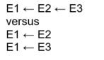
The ON DELETE CASCADE is probably the most common option. The reason is that in data modeling we talk about having “strong” and “weak” entities. A weak entity (such as the Order Details) can exist only if they have a reference back to a strong entity (Orders). You can build chains of weaker and weaker entity references to any depth and spread it out in a tree structure that begins at the strongest entity. Let’s use ← to mean “references” and look at the possible ways you can chain a strong entity, E1, and it’s two weaker entities, E2 and E3.

The difference can be subtle. Imagine that E1 is an order. In the first case, E2 might be order items like a back-to-school supply kit. This kit is made up of individual items (pencils, pens, crayons, paper, etc.) from E3. In this model, you can delete from or add individual items to a kit. Whatever you do, it’s still a back-to-school kit until you remove all the items.

In the second case, E2 might be an order item, and E3 could be delivery options. In theory, you could have an order, E1, that is empty and still deliver it. That doesn’t make much sense in the real world, but it is allowed by the data model.

2) The SET NULL option will change the values in the referencing table to a NULL. Obviously, the referencing column needs to be NULL-able, but the referenced column does not.

3) The SET DEFAULT option will change the values in the referencing table to the default value of that column. Obviously, the referencing column needs to have some DEFAULT declared for it, but each referencing column can have its own default in its own table.

A little-known feature of SQL is the DEFAULT VALUES clause in the INSERT INTO statement where a single row is inserted containing only DEFAULT values for every column. The syntax is: INSERT INTO <table name> DEFAULT VALUES; as a shorthand for INSERT INTO <table name> VALUES (DEFAULT, DEFAULT,… DEFAULT).

4) The NO ACTION option explains itself. Nothing is changed in the referencing table, and a warning message about reference violation might be raised. If a REFERENCES constraint does not specify any ON UPDATE or ON DELETE subclause, then NO ACTION is implicit.

Full ANSI/ISO Standard SQL has more options about how matching is done between the referenced and referencing tables. Full ANSI/ISO Standard SQL also has deferrable constraints. This lets the programmer turn a constraint off during a session so that the table can be put into a state that would otherwise be illegal. However, at the end of a session, all the constraints are enforced. Many SQL products have implemented these options, and they can be quite handy, but I will not mention them anymore. In SQL Server, you have to explicitly turn the constraints on and off with the statement. Please remember to give your constraints names, so this feature will be easy to use.

-- Disable/enable all table constraints
ALTER TABLE <table name> [NOCHECK | CHECK] CONSTRAINT ALL;

-- Disable/enable single constraint
ALTER TABLE <table name> [NOCHECK | CHECK] CONSTRAINT <constraint name>;

It is also possible to use system procedures that will enable or disable all the constraints in the entire database. I can’t give a good reason for wanting to do this, and it sounds likely to be very dangerous.

This weak and strong entity model is very simple. It may not look that way at first, but full E-R modeling can get more elaborate, and it’s tough to support in SQL.

POINTER Chains

I’m probably one of the few people who still remember WATCOM. It was a spinoff from the University of Waterloo in Canada. The University produces some of the best systems programmers I’ve ever worked with, but they could not build a useful human interface. They also produced an SQL compiler which was eventually sold to Sybase.

Their SQL product knew the difference between a referenced and referencing table. The referenced columns in the key were materialized (one way, one place, one time) then the referencing tables built pointer chains back to that occurrence. Basically, they took a lesson from the old network databases (IMS, IDMS, Total, etc.). This meant that no matter how big the key was, the references to it used a simple pointer. It also meant doing joins on primary and foreign keys is fast and cheap (we got really good at scanning pointer chains back in the old network days!). DRI (declarative referential integrity) actions to cascade the updates were also insanely fast; the system simply changed the reference and left the pointers alone.

Similar tricks can be done with SQL products that use hashing and columnar databases. This is one of the reasons that a REFERENCES clause is actually more abstract and is, therefore, nothing like a link.

E-R Modeling

In 1976, Peter Chen introduced Entity-Relationship (E-R) modeling. Variations on his diagramming technique quickly appeared, differing mostly in the graphics. This is still an excellent tool for data modeling today, but it takes a little care to generate DDL from the diagrams.

The basic symbols are fairly simple. Entities are shown by rectangles, relationships among the entities are indicated by a diamond, and connecting lines between the diamonds and rectangles show the relationships. Some simple rules are that a relationship has to apply to one or more entities, that two or more entities in a relationship have to be connected,

and so forth. There are additional symbols to show what kind of relationship the entities have with each other.

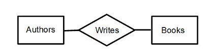
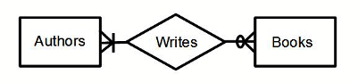
Explaining this is probably easier to do with a simple example. Consider the relationship between authors and their books. The relationship is authorship, or you can just use the verb “write” to keep things simple.

A vertical line means one member of the entity set must be involved in the relationship. Think of the digit one. A circle on the connecting line means no members can be involved; think of a zero.

A “crow’s foot” is the symbol for “many,” which means zero or more. For example, this diagram says at least one, but possibly more authors are involved in the authorship relation. On the books side, there are some options. A circle – crows foot would mean zero or more books are written by the author or authors.

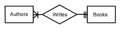
On the other hand, two vertical slashes mean that the author or authors have written precisely one book no more no less.

There have been a few experimental database products that implemented these notations, but SQL is so dominant they never really got anywhere.

WITH CHECK OPTION

A little-used feature in SQL can be used to fake constraints at this level. It is the WITH CHECK OPTION clause on a VIEW that has existed since the SQL–89 standards. To explain this, consider the VIEW

CREATE VIEW V1
AS SELECT col1
  FROM Foobar
 WHERE col1 =’A’;

The view is updatable. This means that it applies to one and only one table that is capable of getting to one and only one row unambiguously. An update like this can be performed:

UPDATE V1 SET col1 =’B’;

The update works just fine, but now rows which were previously returned by the VIEW disappear because they no longer meet the WHERE clause condition. An INSERT statement into the view could also put values into the base table whose rows don’t show up in the VIEW.

The WITH CHECK OPTION makes the system look at the WHERE clause in the VIEW definition. If an insertion or update fails the test, the SQL engine rejects the changes, and the VIEW remains the same. The full ANSI/ISO standard this feature is a more elaborate and includes cascade options.

To fake a constraint, you can use a relatively simple [NOT] EXISTS () constraints on a VIEW to create the conditions. For example, to assure that orders have at least one order item, you can create a VIEW on the join of Orders and Order_Details. This would mean that an order must match to one or more order details to show up in the Orders_2 view. Please note that the base tables are still in the schema. You have to make a decision to use only the VIEW and use DCL to prevent user access to those base tables.

CREATE VIEW Orders_2
AS
SELECT O.order_nbr, ..
  FROM Orders AS O
WHERE EXISTS
 (SELECT *
    FROM Order_Details AS D  
 WHERE D.order_nbr = O.order_nbr)
WITH CHECK OPTION;

Now simply use Orders_2 in your queries. You can still use the base table, Orders. You might want to sit down and play with all the options that you can implement in such a VIEW.

Conclusion

Yes, putting in ER style constraints is a good bit of work for the programmer. But you need to ask yourself is it worth the effort. When do you really need data integrity? Is there any hope in the future for some help from SQL? The answer is yes, and we would find it when we get an implementation of the CREATE ASSERTION statement. This essentially is a CHECK() constraint which applies to the schema as a whole, rather than to columns within a single table. This is why the constraint names are global rather than local.

 

The post Do You Have REFERENCES? appeared first on Simple Talk.

from Simple Talk https://ift.tt/34JQQOd
via

ASP.NET Core with GitOps: Deploying Infrastructure as Code

The series so far:

• ASP.NET Core with GitOps: Dockerizing an API on AWS EC2
• ASP.NET Core with GitOps: Deploying Infrastructure as Code

The first article of the series explained how to create a Docker image of your ASP.NET Core WebApi and deploy it to an existing server. This ensures that you can deploy your application to any server, without having to worry about the software that is installed on it; but you still had to create the server, configure it to accept traffic from port 80, connect to it through SSH and run the Docker image. To follow along with this article, make sure that you have created the Docker image and pushed it to Docker Hub.

By the end of this second article, you will learn how to create your EC2 instance through code, with all the necessary configuration, and deploy the API as part of the process. As explained in the first part of the series, this reduces the risk of your application working in one environment, but failing in another, since you ensure that you always have the same configuration in all environments.

Understanding Infrastructure as Code and CloudFormation

Infrastructure as Code (or IaC) is a way to manage your servers, networks, and other elements of your cloud infrastructure, by writing code instead of manually configuring them.

Most IaC tools offer a way to define your infrastructure by writing in a language like JSON or YAML, in which you can create reusable templates that you can deploy in the cloud. There are many IaC providers out there – Ansible, Azure Automation, Google Cloud Deployment Manager, AWS CloudFormation, etc. Since this series follows all the concepts using AWS, the IaC deployment process will be performed using CloudFormation. However, even on AWS, you can choose other providers, such as Ansible or Chef.

As you will see in this tutorial, CloudFormation works with something called stacks – simply put, collections of resources that you can manage as a single unit (you can read more about it here). CloudFormation currently supports two file types of configuration files: JSON and YAML. The documentation always shows examples in both languages, but the rest of this series will use YAML, as it contains less noise than JSON, making it easier to read and understand.

Each resource has a name, a type, and a list of properties – you can configure resources the same way you would do from the AWS Console. After creating a stack, managing the resources inside it is as simple as updating the file that defines your infrastructure and then performing an update command – this will create any resources that you added in the meantime, update the existing one if necessary, or delete those resources that you eliminated from your code.

Cleaning up is also easy, as deleting the stack will remove all the resources that were part of it, making sure you are not susceptible to any additional costs by forgetting to delete a resource.

What about Elastic Beanstalk?

If you are familiar with AWS, you might have heard about Elastic Beanstalk (EB). If not, you can find an introduction to it here. If you compare its features with what you will learn in this tutorial, it might seem that writing Infrastructure as Code is redundant, since there is a service to do it for you out of the box.

Depending on your purposes, EB might be the way to go for you – it is easier to setup, it offers the scaling capabilities that are going to be touched in this series, and it doesn’t require low-level management of resources.

The reason to use CloudFormation instead of Elastic Beanstalk is being able to have your infrastructure in one place, as a single source of truth, and having the possibility of deploying that anywhere, while also being sure that it will have the intended result.

Prerequisites

Before moving on with CloudFormation, you will need to install the AWS CLI on your machine. This will give you access to working with your resources from the terminal, instead of needing to use the AWS Console in the browser. You can find installation instructions for your OS here. Note that if you install AWS CLI version 2, you will need to change all the commands in the article from aws to aws2.

After successfully installing the CLI, you need to set up an IAM user that will be used to work with your resources.

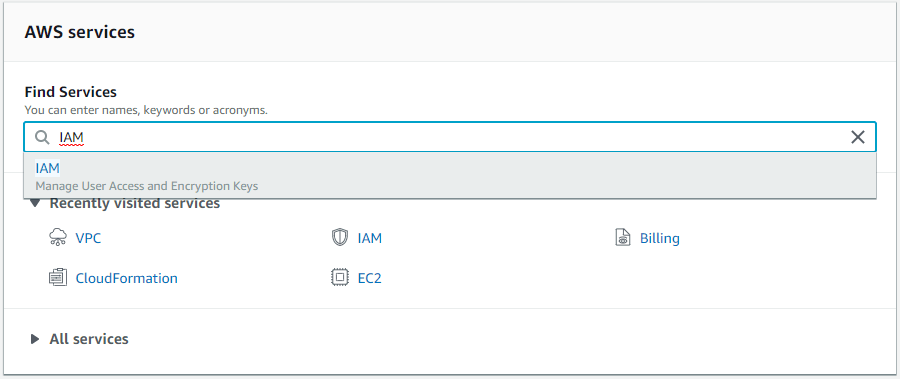
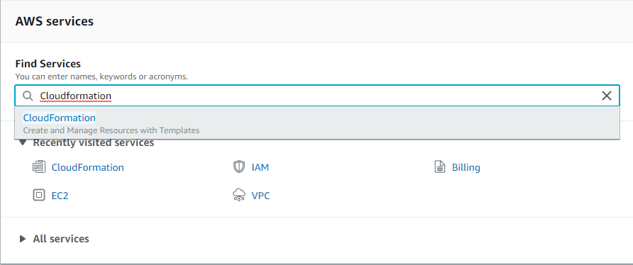
First of all, open the AWS Console and search for IAM in the Find services box.

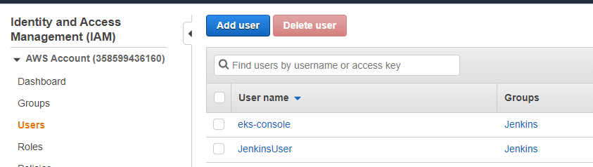
Then, select Users from the left menu and click the Add user button.

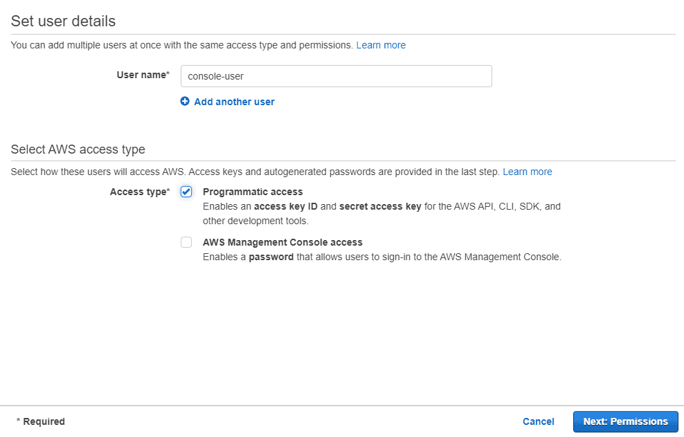
Pick a name, like console-user, for the new user, and check the Programmatic access box. This allows the user to perform actions through the AWS CLI, among other tools from AWS, but it cannot be used to login to the Console. Then, click the Next: Permissions button.

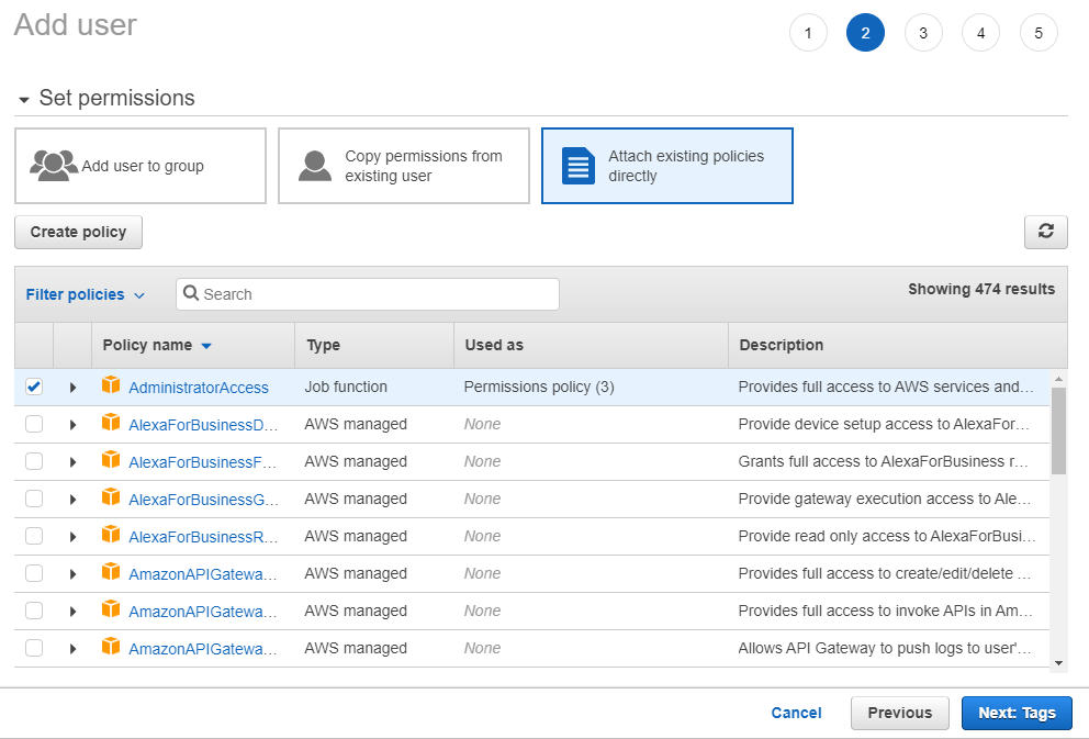
This page allows you to select which actions the user will be able to perform and what resources it can access; it is a good security measure in case someone gains access to your user. Select the Attach existing policies directly and select the AdministratorAccess policy; keep in mind that you should not be doing this in a production scenario, but AWS policies can be tough to work with, so this works for testing purposes. Click the Next buttons and then Create user.

You should now see your newly created user, an access key ID, and a secret access key. In your terminal, run the aws configure command, then paste the required values. For the region, you can use the one that is closest to you from this list, such as eu-central-1.

Make sure that you have also pushed a Docker image to Docker Hub following the instructions in the first article.

Deploying a Single Instance

The first step of deploying your Infrastructure as Code is to find out which resources you need to accomplish your goal. The goal, in this case, is to create an EC2 instance and deploy the previously created Docker image on it.

Once you are aware of what you want to create, the easiest way to gather information is to check the CloudFormation documentation for that resource. Going through the list of properties for the EC2 instance, you can see that none of them is required.

To create the same instance from the previous tutorial, you only need to provide the instance’s image ID. To find the current image ID, go to the EC2 Dashboard and click Launch Instance. Scroll down the list of images until you see the free Ubuntu server. Copy the image ID and save it because you will need to supply it in several scripts.

Click Select to see the sizes. In this case, note t2.micro, which is the free tier. You will be creating your new instance from code, so you can cancel out of the steps after collecting this information.

To write the code to deploy this instance, create a new file called infrastructure.yaml. This is all the code you need, considering you want to deploy an EC2 instance similar to the one from the previous tutorial. Be sure to replace the ImageID property with the image ID you found on the site. Note that you will need to do this each time you copy in a new version of the MainInstance section.

Description: Creating an EC2 instance.
Resources:
  MainInstance:
    Type: AWS::EC2::Instance
    Properties:
      ImageId: ami-0ac05733838eabc06
      InstanceType: t2.micro

After saving the file and modifying the file path if necessary, you can run the following command to deploy your instance to the cloud:

aws cloudformation create-stack --stack-name dotnet-docker --template-body file://infrastructure/infrastructure.yaml

This will return a StackId, so you know the operation has started – it does not mean it was successful, though. The output will look similar to this:

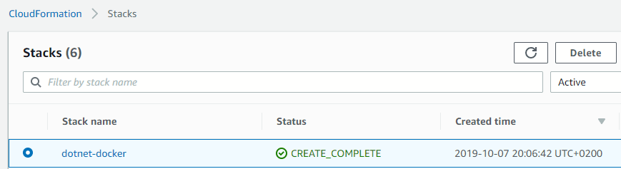
To check on your deployment status, go to the AWS Console and search for CloudFormation in the Find services box.

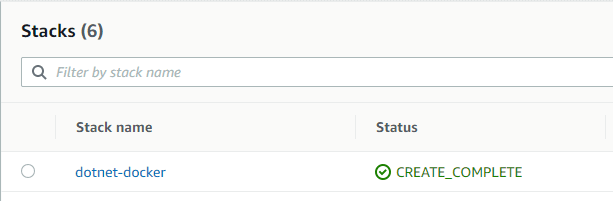
As the stack only contains an EC2 instance, the deployment will complete quite quickly, so you should already see the CREATE_COMPLETE status for your stack.

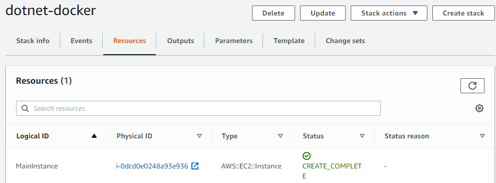
You can click on the stack name and choose the Resources tab to view all the resources inside the stack.

Before pulling and running the Docker image, there is one more thing that needs to be taken care of: allowing the instance to receive (only) HTTP traffic, but to send any type of request. Since you did not provide any security group for the instance, the default one is used – any traffic, to and from any port is allowed; however, this does not provide the level of security and control that you might want for your application.

In the same infrastructure.yaml file, you can define a new resource, SecurityGroup, and then reference it to the instance. However, that is not the only resource that needs to be created, and this is one of the situations where trial and error will lead you to the result. To set the inbound/outbound traffic rules, you need a security group.

MainSecurityGroup:
    Type: AWS::EC2::SecurityGroup
    Properties:
      GroupDescription: Security group for the API instances.
      VpcId: !Ref VPC
      SecurityGroupIngress:
        - IpProtocol: tcp
          FromPort: 80
          ToPort: 80
          CidrIp: 0.0.0.0/0
      SecurityGroupEgress:
        - IpProtocol: tcp
          FromPort: 0
          ToPort: 65535
          CidrIp: 0.0.0.0/0

The security group must link to a VPC to define outbound rules.

VPC:
    Type: AWS::EC2::VPC
    Properties:
      CidrBlock: 192.168.0.0/16
      EnableDnsSupport: true
      EnableDnsHostnames: true

To have your components accessible from the internet, you need an Internet Gateway attached to your VPC.

InternetGateway:
    Type: AWS::EC2::InternetGateway
  InternetGatewayAttachment:
    Type: AWS::EC2::VPCGatewayAttachment
    Properties:
      InternetGatewayId: !Ref InternetGateway
      VpcId: !Ref VPC

Furthermore, you need a way to specify that all the traffic should go to the Internet Gateway you created; for this, you need to create a route table and a route.

RouteTable:
    Type: AWS::EC2::RouteTable
    Properties:
      VpcId: !Ref VPC
  DefaultRoute:
    Type: AWS::EC2::Route
    DependsOn: InternetGatewayAttachment
    Properties:
      RouteTableId: !Ref RouteTable
      DestinationCidrBlock: 0.0.0.0/0
      GatewayId: !Ref InternetGateway

The EC2 is part of the default VPC if not otherwise specified, so the instance and the security group will be part of different VPCs, which means you will not be able to link them; to solve this, you need to create a subnet as part of the new VPC and place the EC2 instance inside that.

Subnet:
    Type: AWS::EC2::Subnet
    Properties:
      VpcId: !Ref VPC
      AvailabilityZone: !Select [ 0, !GetAZs '' ]
      CidrBlock: 192.168.0.0/16
      MapPublicIpOnLaunch: true

Finally, the subnet should be associated with the route table created earlier.

SubnetRouteTableAssociation:
    Type: AWS::EC2::SubnetRouteTableAssociation
    Properties:
      SubnetId: !Ref Subnet
      RouteTableId: !Ref RouteTable

Once everything is added to the file, you can perform an update-stack command to deploy the newly created resources.

aws cloudformation update-stack --stack-name dotnet-docker --template-body file://infrastructure.yaml

Finally, with the infrastructure ready, you can add the commands to install Docker on the machine, login to Docker Hub, pull the image and run it. You do this by adding a property of the EC2 instance, called UserData.

Since these commands contain your password for Docker Hub, which you would not want to be committed to a Git repository, you can use parameters and specify them when creating or updating the stack. This is what the instance code looks like after adding the commands (be sure to replace your image ID).

MainInstance:
    Type: AWS::EC2::Instance
    Properties:
      ImageId: ami-0ac05733838eabc06
      InstanceType: t2.micro
      SecurityGroupIds: 
        - !GetAtt "MainSecurityGroup.GroupId"
      SubnetId: !Ref Subnet
      UserData:
        Fn::Base64:
            !Sub |
                  #!/bin/bash
                  apt-get update -y
                  apt-get install docker.io -y
                  docker login -username ${DockerUsername} -password ${DockerPassword}
                  docker pull docker.io/${DockerUsername}/dotnet-api
                  docker run -d -p 80:80 ${DockerUsername}/dotnet-api

Add the parameters to a special section between Description and Resources.

Parameters:
  DockerUsername:
    Description: The Docker Hub username.
    Type: String
  DockerPassword:
    Description: The Docker Hub password.
    Type: String

If you would like to view the whole file, you can do so here.

To update the stack, you can run the update-stack command with the parameters tag; if you deleted the stack, you can run the create-stack command instead:

aws cloudformation update-stack --stack-name dotnet-docker --template-body file://infrastructure.yaml --parameters ParameterKey=DockerUsername,ParameterValue=yourusername ParameterKey=DockerPassword,ParameterValue=yourpassword

If you go to the EC2 dashboard on the AWS console, you should see a new instance being created. Copy the public DNS and append /api/test to it. You should see the same JSON as in the previous tutorial. Note that if you have problems with the test, see the “Debugging your instances” section later in the article.

Debugging Your Instance

What happens after you deploy your instances, and something does not work as intended – such as the test endpoint not returning anything? The easiest way to figure out what went wrong is to connect to the instance via SSH.

First of all, allow connections to your instances via port 22, by adding another ingress rule to the security group.

MainSecurityGroup:
    Type: AWS::EC2::SecurityGroup
    Properties:
      GroupDescription: Security group for the API instances.
      VpcId: !Ref VPC
      SecurityGroupIngress:
        - IpProtocol: tcp
          FromPort: 80
          ToPort: 80
          CidrIp: 0.0.0.0/0
        - IpProtocol: tcp
          FromPort: 22
          ToPort: 22
          CidrIp: 0.0.0.0/0
      SecurityGroupEgress:
        - IpProtocol: tcp
          FromPort: 0
          ToPort: 65535
          CidrIp: 0.0.0.0/0

Next, in the Instance properties, you have to specify a key-pair name. You can use the one you created during the previous tutorial which you can see by scrolling down to the Network & Security section of the ECW menu.

MainInstance:
    Type: AWS::EC2::Instance
    Properties:
      KeyName: dotnet-docker-keypair
      ImageId: ami-0ac05733838eabc06
      InstanceType: t2.micro
      SecurityGroupIds: 
        - !GetAtt "MainSecurityGroup.GroupId"
      SubnetId: !Ref Subnet
      UserData:
        Fn::Base64:
            !Sub |
                  #!/bin/bash
                  apt-get update -y
                  apt-get install docker.io -y
                  docker login -username ${DockerUsername} -password ${DockerPassword}
                  docker pull docker.io/${DockerUsername}/dotnet-api
                  docker run -d -p 80:80 ${DockerUsername}/dotnet-api

The update-stack command will not achieve the intended result here, as the instance is already running. Instead, delete your stack first, by running this code.

aws cloudformation delete-stack --stack-name dotnet-docker

Then create it again with the new configuration.

Afterwards, you can follow the connection technique that you used for the instance created manually in the first article, by the SSH command. Make sure that the pem file is in a secured location.

ssh -i "dotnet-docker-keypair.pem" ubuntu@{public-dns}

Once you are connected, you can check the logs for any issues that might have appeared while launching the instance, by running the following command.

cat /var/log/cloud-init-output.log

Don’t forget that this method is something to be used for testing and debugging purposes only – remove such configurations when deploying production environments.

Deploying Multiple Instances

If you remember the series introduction, one of the essential aspects was being able to deploy multiple, identical servers that run the same API. This way, if one of them fails, or if there is an update for the API, the customers are still able to use the service by being redirected to the working instances.

The goal of working with multiple instances is to make it seem like the users are only interacting with one server. For this purpose, a load balancer will be placed in front of the instances – this will receive the traffic and decide where to send it, ensuring a lower response time for the clients.

To achieve the deployment of multiple instances, there are some new resources that need to be added to the infrastructure:

Additional subnets for different availability zones in your region; this ensures that if one availability zone fails, your API is still up and running; the Subnet and the SubnetRouteTableAssociation sections created previously should be deleted.

Subnet1:
    Type: AWS::EC2::Subnet
    Properties:
      VpcId: !Ref VPC
      AvailabilityZone: !Select [ 0, !GetAZs '' ]
      CidrBlock: 192.168.0.0/24
      MapPublicIpOnLaunch: true
  Subnet2:
    Type: AWS::EC2::Subnet
    Properties:
      VpcId: !Ref VPC
      AvailabilityZone: !Select [ 1, !GetAZs '' ]
      CidrBlock: 192.168.1.0/24
      MapPublicIpOnLaunch: true
  Subnet1RouteTableAssociation:
    Type: AWS::EC2::SubnetRouteTableAssociation
    Properties:
      SubnetId: !Ref Subnet1
      RouteTableId: !Ref RouteTable
  Subnet2RouteTableAssociation:
    Type: AWS::EC2::SubnetRouteTableAssociation
    Properties:
      SubnetId: !Ref Subnet2
      RouteTableId: !Ref RouteTable

A Launch Configuration, that represents the template for any instance that is going to be created; since you are not creating the instances manually anymore, this will specify the image id, the size and the user data for your servers; as part of this step, you must also delete the EC2 instance code (MainInstance section). This section contains the Image ID, so be sure to replace it.

LaunchConfiguration:
    Type: AWS::AutoScaling::LaunchConfiguration
    Properties:
      UserData:
        Fn::Base64: !Sub |
          #!/bin/bash
          apt-get update -y
          apt-get install docker.io -y
          docker login -u ${DockerUsername} -p ${DockerPassword}
          docker pull docker.io/${DockerUsername}/dotnet-api
          docker run -d -p 80:80 ${DockerUsername}/dotnet-api
      ImageId: ami-0ac05733838eabc06
      SecurityGroups:
      - Ref: MainSecurityGroup
      InstanceType: t2.micro

An Auto Scaling Group to control how many instances are created, when to create them and when to stop them.

AutoScalingGroup:
    Type: AWS::AutoScaling::AutoScalingGroup
    Properties:
      VPCZoneIdentifier:
         - !Ref Subnet1
         - !Ref Subnet2
      LaunchConfigurationName:
        Ref: LaunchConfiguration
      DesiredCapacity: 3
      MinSize: 2
      MaxSize: 4
      TargetGroupARNs:
      - Ref: TargetGroup

A Load Balancer that will control the traffic for the instances inside the Auto Scaling Group.

LoadBalancer:
    Type: AWS::ElasticLoadBalancingV2::LoadBalancer
    Properties:
      Subnets:
      - !Ref Subnet1
      - !Ref Subnet2
      SecurityGroups:
      - Ref: MainSecurityGroup

A Load Balancer Listener and a rule for it, as well as a Target Group, to specify how to check the health of each instance and make sure they are still running. Here is the Listener Rule section:

ListenerRule:
    Type: AWS::ElasticLoadBalancingV2::ListenerRule
    Properties:
      Actions:
      - Type: forward
        TargetGroupArn: !Ref TargetGroup
      Conditions:
      - Field: path-pattern
        Values: [/]
      ListenerArn: !Ref Listener
      Priority: 1

Add the Listener.

Listener:
    Type: AWS::ElasticLoadBalancingV2::Listener
    Properties:
      DefaultActions:
      - Type: forward
        TargetGroupArn:
          Ref: TargetGroup
      LoadBalancerArn:
        Ref: LoadBalancer
      Port: '80'
      Protocol: HTTP

Also add the TargetGroup section.

TargetGroup:
    Type: AWS::ElasticLoadBalancingV2::TargetGroup
    Properties:
      HealthCheckIntervalSeconds: 10
      HealthCheckPath: /
      HealthCheckProtocol: HTTP
      HealthCheckTimeoutSeconds: 8
      HealthyThresholdCount: 2
      Port: 80
      Protocol: HTTP
      UnhealthyThresholdCount: 5
      VpcId: !Ref VPC

You can view the file containing all the resources here.

From the CloudFormation Stacks list, delete the original stack. You should now run the same command from earlier with create-stack and the username and password parameters. Once it finishes (and it might take longer than the previous versions, since there are many new resources added), go to the EC2 dashboard on AWS Console to inspect the resources. You should see three instances.

You can go to any of them, copy the public DNS and append /api/test to it, and receive the expected JSON message from earlier. This ensures that all the instances work as expected.

While on the instances page, if you scroll down in the left menu and select Load Balancers, you should see one resource.

Below, you should see a property called DNS Name, which is the URI for your load balancer. You can copy it, append /api/test and receive the same JSON message as from the instances. You are done!

Debugging Your Instances

Enabling SSH connections to your instances is essentially the same process as the one described earlier, for the single instance – however, the key-pair will be added to the launch configuration and propagated to all the EC2 instances.

The first step is adding port 22 as an ingress rule for the security group.

MainSecurityGroup:
    Type: AWS::EC2::SecurityGroup
    Properties:
      GroupDescription: Security group for the API instances.
      VpcId: !Ref VPC
      SecurityGroupIngress:
        - IpProtocol: tcp
          FromPort: 80
          ToPort: 80
          CidrIp: 0.0.0.0/0
        - IpProtocol: tcp
          FromPort: 22
          ToPort: 22
          CidrIp: 0.0.0.0/0
      SecurityGroupEgress:
        - IpProtocol: tcp
          FromPort: 0
          ToPort: 65535
          CidrIp: 0.0.0.0/0

Next, in the Launch Configuration properties, specify the key-pair name.

LaunchConfiguration:
    Type: AWS::AutoScaling::LaunchConfiguration
    Properties:
      KeyName: dotnet-docker-keypair
      UserData:
        Fn::Base64: !Sub |
          #!/bin/bash
          apt-get update -y
          apt-get install docker.io -y
          docker login -u ${DockerUsername} -p ${DockerPassword}
          docker pull docker.io/${DockerUsername}/dotnet-api
          docker run -d -p 80:80 ${DockerUsername}/dotnet-api
      ImageId: ami-0ac05733838eabc06
      SecurityGroups:
      - Ref: MainSecurityGroup
      InstanceType: t2.micro

Again, don’t forget to remove these settings before deploying your instances to production!

Cleaning Up

If you are following this just for testing or learning purposes, you should avoid keeping the resources alive for too long, as it can create additional costs or reach the free tier limits; since all the resources are part of a stack, deleting them is as simple as deleting the stack. You can do it from the console, by running.

aws cloudformation delete-stack --stack-name dotnet-docker

You can also remove the stack from the CloudFormation dashboard in the AWS Console, by selecting the stack and clicking the Delete button.

What is Next?

It might seem that the goal of the tutorials is more or less achieved: you can pack the code from your Git repository in a Docker image and deploy it to multiple instances, ensuring the high availability of your application. But you are still handling most of this process manually.

Going forward, you will learn how to use Kubernetes to orchestrate your Docker containers, and how to automate the deployment process.

 

The post ASP.NET Core with GitOps: Deploying Infrastructure as Code appeared first on Simple Talk.

from Simple Talk https://ift.tt/34Hfzmr
via