Wednesday, May 20, 2020

Tackle Big-O Notation in .NET Core

Performance sensitive code is often overlooked in business apps. This is because high-performance code might not affect outcomes. Concerns with execution times are ignorable if the code finishes in a reasonable time. Apps either meet expectations or not, and performance issues can go undetected. Devs, for the most part, care about business outcomes and performance is the outlier. When response times cross an arbitrary line, everything flips to less than desirable or unacceptable.

Luckily, the Big-O notation attempts to approach this problem in a general way. This focuses both on outcomes and the algorithm. Big-O notation attempts to conceptualize algorithm complexity without laborious performance tuning.

In this take, I’ll delve into Big-O notation and how to apply this in .NET. I’ll begin with theory found in intro to computer programing courses. Then, dive into examples based on real-world code. In the end, this guides through the creative process of writing algorithms that use sound theory.

I’ll stick with proven tools such as .NET Core 3.1.100, the recommended LTS version for now. Code samples can run in the latest version of Visual Studio 2019. I’ll add BenchmarkDotNet to the project to verify execution times. This makes undetectable performance issues visible. You can download the sample code from GitHub.

Feel free to follow along, to fire up a new project with the CLI do:

dotnet new console

Be sure to do this inside of a project folder such as TackleBigONetCore. This same step is possible in Visual Studio. Because I do not wish to put you through a click hunt, I’ll stick to the CLI.

Then, be sure to add the benchmark tool:

dotnet add package BenchmarkDotNet --version 0.12.0

Before I lay down a single line of code, it is best to start with theory.

What Is Big-O Notation?

The Big-O notation measures the worst-case complexity of an algorithm. The algorithm works on data input of any size. For a given n, it answers the question: “What happens as n approaches infinity?” This helps to analyze the effectiveness of an algorithm which can be measured in time and space. Think of time as the execution time, and space as the input dataset size which consumes memory.

The algorithmic analysis gets summed up using Big-O notation, for example, O(1) for constant time. There are three main ways to do an analysis:

  • O(1): For constant time because it does not change based on input space
  • O(n): For linear time because it assumes n operations in the worst-case scenario
  • O(n2): For quadratic time which shows exponential time degradation in the worst-case scenario
  • O(n3): For cubic time, like O(n2) with exponentially greater time complexity

I’ll come back to each one as code samples get fleshed out. For now, think of algorithm complexity as a function like f(n). Input size n represents the number of inputs, f(n)time represents the time it takes, and f(n)space shows memory usage. Big-O notation comes with rules to help programmers analyze f(n). In academia, there are a lot of rules one might encounter, but I’ll focus on the most relevant:

  • Coefficient rule: For any constant k > 0, if kf(n) then the result is O(g(n)). This rule eliminates coefficients that multiply results from input size. This is because as n approaches infinity, coefficients become negligible.
  • Sum rule: If f(n) is O(h(n)), and g(n) is O(p(n)), then f(n) + g(n) is O(h(n) + p(n)). In practice the sum rule adds up two algorithms that are similar in time and space. For example, f(n) + f(n) can be 2f(n) from which applies the coefficient rule.
  • Product rule: If f(n) is O(h(n)), and g(n) is O(p(n)), then f(n)g(n) is O(h(n)p(n)). For algorithms similar in time and space, the product rule may result in O(n) = n2. For example, nested loops that multiply which results in quadratic time.

The following shows common Big-O notations from an algorithmic analysis:
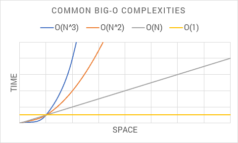
I recommend committing these complexities to memory in your mind’s eye. As I venture through each Big-O complexity, keep this chart in mind. This helps to visualize implications as time and space exponentiate with each complexity.

With all this Big-O theory out of the way, time to put this to good use.

Lab Rats

For this project, I’ll create a contrived use case of lab rats racing three at a time in several mazes. The goal is to imagine a data model useful for algorithmic analysis. Each Big-O complexity corresponds with each dataset.

This can go anywhere in the project. Because the emphasis is on benchmark analysis, I’ll put this inside a BigOBenchmarks class.

First, create a maze that has lab rats going three at a time:

class Maze
{
  public int MazeNumber { get; set; }
  public Difficulty Difficulty { get; set; }
  public int LabRat1 { get; set; }
  public int LabRat2 { get; set; }
  public int LabRat3 { get; set; }
}

enum Difficulty
{
  Easy,
  Medium,
  Hard
}
Now for many lab rats in each maze:
class LabRat
{
  public int TrackingId { get; set; }
  public Color Color { get; set; }
}

enum Color
{
  Black,
  White,
  Gray
}

Lastly, this encapsulates race data:

class Race
{
  public int MazeNumber { get; set; }
  public int Participant { get; set; }
  public FinishTime FinishTime { get; set; }
}

enum FinishTime
{
  Fast,
  Average,
  Slow
}

This completes the domain, there are many mazes, with many lab rats in groups of three, with many races. The rest of the BigOBenchmarks class looks like this:

public class BigOBenchmarks
{
  private const int N = 999;

  private readonly IList<LabRat> labRats;
  private readonly IList<Maze> mazes;
  private readonly IList<Race> races;

  public BigOBenchmarks()
  {
  }

  [Benchmark]
  public int DummyBenchmark()
  {
    return 0;
  }
}

Leave the constructor empty for now, as this is where you initialize benchmark data. I’ll come back to each benchmark method. For now, be sure to return a value. This way the compiler does not optimize the whole benchmark method out. Methods decorated with Benchmark are part of the benchmark result. The Benchmark attribute is in this namespace:

using BenchmarkDotNet.Attributes;

For this analysis, I’m keeping data input size N set to about a thousand. Because lab rats go three at a time, this leaves around three hundred mazes.

To flesh out BenchmarkDotNet so that benchmarks execute, crack open Program in the console project and add this:

BenchmarkRunner.Run<BigOBenchmarks>();

Be sure to include the namespace:

using BenchmarkDotNet.Running;

The project runs with dotnet watch run -c Release. BenchmarkDotNet works on Release because Debug can be one hundred times slower. Running this in watch mode makes it to where benchmarks run at each save. Next, time to look at each Big-O complexity based on data.

Big-O O(n) Linear Time

Knock out DummyBenchmark as I’ll need room for meaningful benchmarks. Say I want to pluck a single lab rat from the dataset. Start by initializing the data in the constructor:

labRats = new List<LabRat>(N);
for (var i = 0; i < N; i++)
{
  labRats.Add(new LabRat
  {
    TrackingId = i,
    Color = (Color)(i % 3)
  });
}

Note the use of N as a constructor parameter when I initialize this list of lab rats. This sets the Capacity in the internal data structure. If the data input size is known, I recommend letting .NET know too. With the data in place, the traditional way to pluck a single item in .NET is using First. Be sure to add System.Linq to the using statements:

var result = labRats.First(d => d.TrackingId == N - 1);

return (int)result.Color;

Be sure to place this inside a benchmark method to verify what’s happening. To the untrained eye, this may seem like a simple operation without dings in performance. But it is O(n) or linear time complexity. This is because Big-O assumes the worst-case scenario, and this means looping through a whole dataset. In .NET, First picks the first match that exists, but Big-O must assume worst-case. In a worst-case scenario, the first match goes at the end. This frees the programmer from analysis paralysis when studying algorithms. By assuming worst-case, there is less cognitive load when thinking about algorithmic complexity.

Benchmark results are as follows:

This runs on avg for 15 microseconds given a sample size of about a thousand. The key takeaway is how this executes in microseconds. Because Big-O is either exponentially better or worse it will run in different time units. For this reason, I recommend executing one benchmark at a time for better results.

Big-O O(n2) Quadratic Time

This time I’ll need a set of mazes, go back in the BigOBenchmarks constructor and initialize maze data:

mazes = new List<Maze>(N / 3);
for (var i = 0; i < N / 3; i++)
{
  mazes.Add(new Maze
  {
    MazeNumber = i,
    Difficulty = (Difficulty)(i % 3),
    LabRat1 = i,
    LabRat2 = i + N / 3,
    LabRat3 = i + N / 3 * 2
  });
}

Maze data is but a third of lab rat data in space complexity. As data input size approaches infinity, this difference becomes negligible. This is because both datasets share similar time and space complexities.

Say, for example, I want to pluck a lab rat and check which maze difficulty it finished. A solution is:

var result = 0;

foreach (var maze in mazes)
{
  var rat = labRats.First(r => r.TrackingId == N - 1);

  result = maze.LabRat3 == rat.TrackingId ? 
                   (int)maze.Difficulty : result;
}

return result;

Be sure to put this in a benchmark, and one takeaway is the nested loops. Because of the product rule, this makes the complexity O(n2). The outer loop goes through each maze, and the inner loop plucks a lab rat via iteration. Conceptually, nested loops on input data size n have a multiplicative effect. If the outer loop has n items, it permutates through all items in both loops. If, for example, there are 100 items, nested loops iterate 100×100 for a grand total of 10,000.

These are the results:

This time results are in milliseconds. Remember the chart I showed earlier? It shows this same exponential degradation. As complexity grows in Big-O, there are performance implications to the algorithm.

One way to tackle Big-O complexity is with a lookup table like IDictionary<>. Instead of having to iterate through lab rats, it is possible to pick one. A lookup table does a one-to-one mapping with a given key. Lookup mapping has a constant time complexity regardless of input data size. This reduces complexity back down to O(n).

Add a lookup table with a .NET dictionary to the benchmark class as a private instance variable:

private readonly IDictionary<int, LabRat> labRatLookup;

Because First was doing matches against the id, the lookup table uses this as the key. Initialize the lookup dictionary in the class constructor:

labRatLookup = labRats.ToDictionary(l => l.TrackingId);

Now, run another benchmark with this algorithm:

var result = 0;

foreach (var maze in mazes)
{
  var rat = labRatLookup[N - 1];

  result = maze.LabRat3 == rat.TrackingId ? 
       (int)maze.Difficulty : result;
}

return result;

Both solutions are identical, minus the nested loop and complexity. The lookup table uses the same id First once used. So, this does not affect the outcome of the algorithm.

Benchmark results are now:

Big-O O(n3) Cubic Time

Welcome to the fray, algorithms of this complexity tend to choke on modest size datasets. The time complexity is higher relative to the data input size.

In the constructor, initialize rat race data:

races = new List<Race>(N);
for (var i = 0; i < N; i++)
{
  races.Add(new Race
  {
    MazeNumber = i % (N / 3),
    Participant = i,
    FinishTime = (FinishTime)(i % 3)
  });
}

This time find race finish time by cross-referencing all other data points:

var result = 0;

foreach (var maze in mazes)
{
  foreach (var rat in labRats)
  {
    var race = races.Where(r => r.MazeNumber == N / 3 - 1).ToArray();

    result = maze.MazeNumber == race[2].MazeNumber
      && rat.TrackingId == race[2].Participant
      ? (int)race[2].FinishTime : result;
  }
}

return result;

In .NET, Where returns any items that match the predicate. This also means looping through the entire dataset. Given the product rule with three nested loops, this spikes complexity to O(n3).

Benchmarks results are as follows:

Wow, this breaks the second barrier, execution times are dismal. Because customers don’t like to wait, this gets into unacceptable levels. Note data input size is in the hundreds, which is not that big at all. As data input size increases, count on this getting exponentially slower.

One way to tackle this much complexity in .NET is with ILookup<>. This Where throws a kink because it can return any number of items. What’s good is this returns arrays of constant size because lab rats go in groups of three. This makes the algorithm 3f(n), applying the coefficient rule, this brings it to constant time.

Declare this lookup table as a private instance variable in the class:

private readonly ILookup<int, Race> raceLookup;

Then, initialize race lookup data in the constructor:

raceLookup = races.ToLookup(r => r.MazeNumber, r => r);

This makes MazeNumber the key from which we get the array with three items. This is the same predicate found in the where clause. By preserving the where clause in the key, it keeps the outcome the same. The lab rat lookup can go in here too to further optimize complexity. Now tweak the algorithm as follows:

var result = 0;

foreach (var maze in mazes)
{
  var race = raceLookup[N / 3 - 1].ToArray();
  var rat = labRatLookup[race[2].Participant];

  result = maze.MazeNumber == race[2].MazeNumber
    && rat.TrackingId == race[2].Participant
    ? (int)race[2].FinishTime : result;
}

return result;

Note there are two lookups side-by-side, one for races and one for rats. Because time and space complexities are similar, applying the sum rule, this gets a 2f(n). Big-O rules combine, so, applying the coefficient rule keeps lookups at constant time. Because this loops through mazes, the complexity is O(n).

I want to hear a drumroll please, time to check benchmarks results:

This brings execution time back down to microseconds and way within an acceptable range. Note the exponential gains from more than a second to tens of microseconds. Going from cubic time down to linear time does make an astronomical difference. For business apps, this kind of performance is “good enough.” Any further optimization is likely too pedantic for the working programmer.

Big-O O(1) Constant Time

The keen reader may notice lookup tables dominate complexity gains, so why not get rid of looping? Should be interesting to see how this stacks up given the theory. Lookup tables are constant time because of this one-to-one relationship. The computer has an easier time with this because it knows where to find this in memory. When a lookup returns many items, the coefficient rule keeps complexity constant if the array is of constant size.

To eliminate looping, what is missing is a maze lookup:

private readonly IDictionary<int, Maze> mazeLookup;

Go in the constructor and add:

mazeLookup = mazes.ToDictionary(l => l.MazeNumber);

Then, tweak the algorithm so it no longer loops:

var race = raceLookup[N / 3 - 1].ToArray();
var rat = labRatLookup[race[2].Participant];
var maze = mazeLookup[race[2].MazeNumber];

var result = maze.MazeNumber == race[2].MazeNumber
  && rat.TrackingId == race[2].Participant
  ? (int)race[2].FinishTime : 0;

return result;

Below are the results:

Success, performance should remain the same regardless of data input size. This execution time breaks into the nanosecond range. This is exponentially faster than anything I’ve shown before. This follows Big-O theory with good precision, so it is trustworthy.

A similar feat is possible with caching but with some gotchas. Caching large chunks of data and then looping does nothing for performance. When the cache lives outside memory and over the network in another box, large datasets must be deserialized, which spike complexity. This is one reason why caching is not a performance silver bullet. It’s only by caching a narrow slice with a one-to-one lookup that any real gains come in.

Conclusion

Big-O notation has a nice way to encapsulate algorithmic complexity. As algorithm complexity grows performance exponentially degrades. Looping spikes complexity and nested loops exponentiate this complexity. .NET provides lookup tables to quell this complexity such as IDictionary<>, and ILookup<>. Reducing complexity to constant time is the best optimization possible.


The post Tackle Big-O Notation in .NET Core appeared first on Simple Talk.


from Simple Talk https://ift.tt/36l4p8r
via

Key Insights from the 2020 State of SQL Server Monitoring Report

This marks the third year that Redgate have launched a survey to better understand how organisations monitor their databases. This year, 971 database professionals from around the world responded.

Here are some of the key insights from the survey:

Estates are growing more than ever

Companies who reported over 1,000 SQL Server instances grew 9% year-on-year while those reporting fewer than 100 instances have dropped for a second year. This trend is no surprise as organisations store more data digitally and find more ways to utilise that data. DBA teams are responsible for more servers than ever, and a using monitoring solution is the only way to manage so many servers since manually checking each one on a regular basis would be impossible. 

Cloud adoption is increasing rapidly

The respondents of the survey reported increased adoption of the cloud, especially Azure and Oracle DB Cloud service. As these services mature and become more affordable, this trend will likely continue. Database monitoring tools that monitor both servers on-premises and databases like Azure SQL Database in one view can save DBAs time.

Performance, migrations, and recruitment are all challenges this year

Database administrators often spend time resolving performance issues, and this year it was reported as the most significant overall challenge. Performance one of the most critical areas that database monitoring will be of assistance. With monitoring, DBAs can watch trends and correct small problems before they become big issues. With a monitoring tool in place, new members of the team can be productive more quickly.

Humans cause problems

Human error and ad-hoc user access were cited as the cause of problems by almost half of the respondents. This is another area where monitoring can help. With monitoring, DBAs can find bad queries that cause tempdb to grow or be notified when a new login is added to sysadmins, for example.

Monitoring is key to Database DevOps success

The respondents of the survey reported a 28% reduction in Mean Time To Detection (MTTD) of deployment issues and a 22% reduction in Mean Time To Recovery (MTTR) when they use a third-party monitoring tool. With monitoring in place, it’s easy to see changes in performance after a deployment and figure out what went wrong.

Once again, the respondents reported that having a monitoring tool in place allows DBAs to spend less time looking at server health daily. This allows them to spend more time on activities like project work and automation, therefore, bringing more value to the organisation and their customers.

If you would like to take a look at the report, you can download it here, and we encourage you to participate next year.

Commentary Competition

Enjoyed the topic? Have a relevant anecdote? Disagree with the author? Leave your two cents on this post in the comments below, and our favourite response will win a $50 Amazon gift card. The competition closes two weeks from the date of publication, and the winner will be announced in the next Simple Talk newsletter.

The post Key Insights from the 2020 State of SQL Server Monitoring Report appeared first on Simple Talk.


from Simple Talk https://ift.tt/36nGw0c
via
Thursday, May 14, 2020

How to Add Help to PowerShell Scripts

Shortly after writing my last article on Parameters, I had to update a script, and I wanted to make it easier for others to run. One of the features I wanted to add was the ability to show them what the script would do with the provided parameters without actually running the script, in other words, provide “help”.

Using a Switch to Control Help

My initial thought was to add another parameter, make it a Boolean and then check the state of it. If it’s true, display some help text. If not, run the code. However, like many things, the creators of PowerShell thought of a solution that’s even easier that I’ll get to later.

To keep things simple, I’ll start with the naïve example. (note I’ve started using Visual Studio Code to develop my PowerShell and but also still use the deprecated PowerShell ISE IDE, so my examples may come from either.)

Save this script as Boolean_help.ps1.

param([boolean] $help )
#
# Author: Greg D. Moore
# Date: 2020-02-18
# Version: 1.0
# Show boolean help
#
if ($help -eq $true)
{
    write-host "This is help for this program. It does nothing. Hope that helps."
}
else
{
    write-host "Do nothing."
}

To run it, simply navigate to the folder where it’s saved and execute it.

.\Boolean_help.ps1

Since you haven’t supplied a value for the $help parameter, your output should be:

If you add a $true value as follows, you will see your help message.

.\Boolean_help.ps1 $true

Here are the results.

That’s a step in the right direction, but it’s not quite good enough. What if your next user who isn’t overly PowerShell savvy tries to use it and does something like the following or other variations?

.\Boolean_help.ps1 -help true

Your user may get frustrated trying to get help from your script. Fortunately, PowerShell provides a different and, in my opinion, a far superior way of handling certain conditionals, and that’s with a data type known as switch.

Enter the following script and save it as Switch_help.ps1.

param([switch] $help )
#
# Author: Greg D. Moore
# Date: 2020-02-18
# Version: 1.0
# Show switch help
#
if ($help)
{
    write-host "This is help for this program. It does nothing. Hope that helps."
}
else
{
    write-host "Do nothing."
}

Here, instead of defining $help as a Boolean, it is now a switch datatype. The switch acts similar to a Boolean, but not quite.

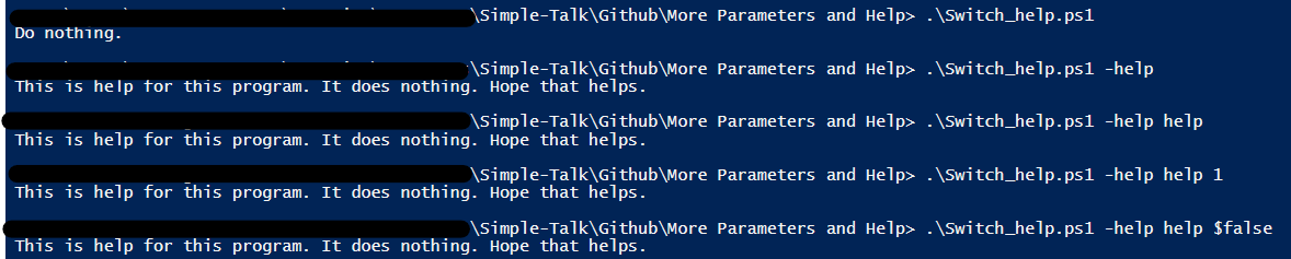
Run the following, and you will see what I mean.

.\Switch_help.ps1
.\Switch_help.ps1 -help
.\Switch_help.ps1 -help help
.\Switch_help.ps1 -help help 1
.\Switch_help.ps1 -help help $false

As you can see, it doesn’t really matter what value you put after the –help parameter. As long as the parameter itself is referenced when the script is called, it will have the value of $true.

It should also be clear that the switch datatype isn’t limited to just help. You can use it for enabling or disabling other items. For example, you might want to have a parameter called $debug, which would allow you to enable debug information. This is a great place for the use of the switch parameter.

However, you may already realize that the help provided above isn’t in the format that most cmdlets provide. I will come back to that later in this article, but first, take a look at some other options with parameters that will help those who run your code.

Adding Default Parameters

I don’t know about you, but if I can, I like to make it harder to make mistakes. One way of doing that is to provide a fixed set of default parameters. For example, you might have a script that can only run against a fixed set of servers.

Enter the following script and save it as Defaults.ps1.

param([parameter(mandatory)] [validateset("ProdDB_Server","DevDB_Server")] [string] $dbserver )
write-host "You picked $dbserver!"

Now, I have to take a slight detour and mention one limitation of Visual Code Studio for development is that, at the time of this writing, I have not found a way to have it automatically pop-up parameters and possible defaults. For the following example, I recommend using the PowerShell ISE to see how this can work. If you enter the script name and the parameter –dbserver and then space, you should see a small pop-up

.\Defaults.ps1 -dbserver

If you select one of those two items, the script will run as you expect.

Obviously, if you add another server, for example, a UAT server, you’d have to update the script. But, by using validated parameters, you ideally avoid a user from entering an invalid server name here.

Also, if you do try to type in an option not allowed, you will get an error message.

.\Defaults.ps1 -dbserver UATDBserver

Conflicting Defaults

If you start to use default parameters, you may suddenly find yourself with required parameters that conflict with each other. For example, if you are using scripts to deploy code (and if you’re not, you should be) you might find in some cases you want to deploy to an environment, but other times to a specific database.

Now, you could write a script that takes both mandatory parameters and then tries to figure out what you want, but there’s an easier way. Enter the following:

param([parameter(mandatory, ParameterSetName='ByEnvironment')] [validateset("ProdDB_Server","DevDB_Server")] [string] $dbserver, 
[parameter(mandatory, ParameterSetName='ByDatabase')] [validateset("sales","product")] [string] $database ) 
if ($dbserver)
{
    Write-Host "Your code will be deployed to the $dbserver server"
}
if ($database)
{
    Write-Host "Your code will be deployed to the $database database"
}

And save it as Conflicting_Parameters.ps1.

When you try to run it, you will find you can decide whether you want to deploy to a specific server using the $dbserver parameter OR to a specific database using the $database parameter. For example, you may want to initially want to deploy a new script to your dev server, and once tested to your production server, or, in the second case, you may want to deploy the script to a specific database across all your servers at once.

.\Conflicting_Parameters.ps1 -database product
.\Conflicting_Parameters.ps1 -dbserver DevDB_Server

Save the following script as Conflicting_Parameters_2.ps1:

param([parameter(mandatory, ParameterSetName='ByEnvironment')] [validateset("ProdDB_Server","DevDB_Server")] [string] $dbserver, 
[parameter(mandatory, ParameterSetName='ByDatabase')] [validateset("sales","product")] [string] $database, 
[parameter(mandatory, ParameterSetName='ByEnvironment')] [validateset("Europe","North America","All")] [string] $region,
[string] $comment) 
if ($dbserver)
{    
    Write-Host "Your code will be deployed to the $dbserver server in the $region region."
}
if ($database)
{
    Write-Host "Your code will be deployed to the $database database"
}
if ($comment)
{
    Write-host "Your comment was: $comment"
}

You will note several major changes. You now have two parameters, $dbserver and $region that are both part of the same Parameter Set ByEnvironment. Note that they’re separated by the $database parameter. This should make it clear, that the ParameterSetName is what ties them together, not their placement in the list of parameters. Also, you will note that there is a final optional parameter, $comment that is not tied to either Parameter Set.

The $comment parameter can be optionally used with either Parameter Set.

Adding Better Help

As noted above, the first and most obvious solutions for providing help that come to mind are the ones mentioned at the start of the article. However, like most things, PowerShell provides a better way of handling this.

First, your scripts already might give help if parameters. Simply try this:

get-help .\Conflicting_Parameters_2.ps1

You should see:

So that’s a start.

But it might be nice to actually let users know what the parameters, like –region, mean.

Take the script Conflicting_Parameters_2.ps1 and save it as Conflicting_Parameters_Help1.ps1.

Then add the following block of code as the first lines of the script:

<#
.Description
This is a test file to demonstrate conflicting parameters.
#>

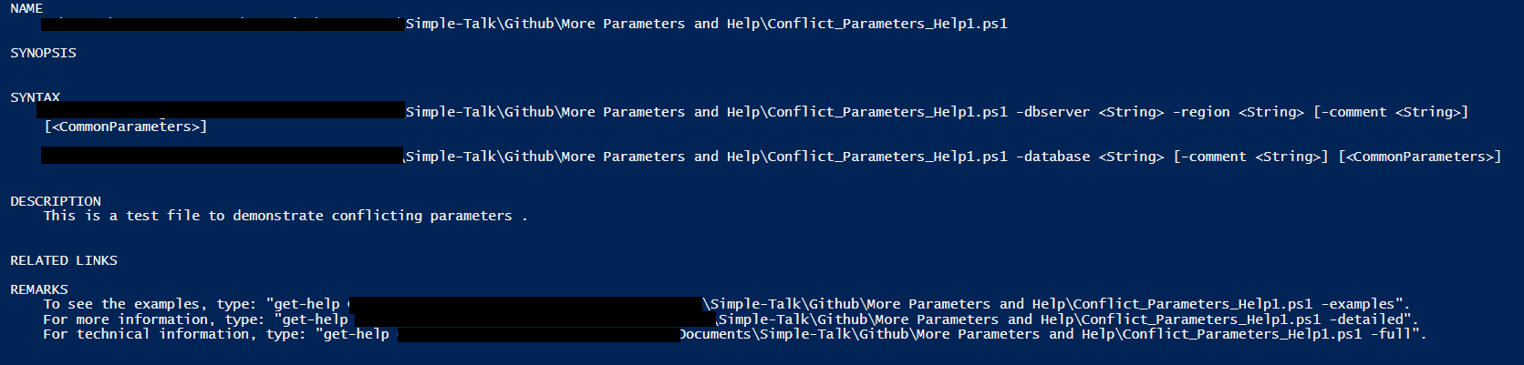
Save this and then run:

get-help .\Conflict_Parameters_Help1.ps1

You should see something very similar to:

Now, this is starting to look a bit more like a real script!

But you haven’t solved the problem of giving useful examples about what the parameters can or should be. Fortunately, that’s easy to fix with the addition of the following lines. Add these and save as Conflicting_Parameters_Help2.ps1.

.PARAMETER dbserver
Determines if you are deploying to the Production or Dev DB server. Valid values are ProdDB_Server or DevDB_Server
Must be used with the region parameter. May not be used with the database parameter

.PARAMETER database
Determines if you are deploying to the Sales or Product database. Valid values are sales or product
May not be used with the dbServer and region parameters

.PARAMETER region
Determines which region you are deploying to. Valid values are Europe, North America or All
Must be used with the dbserver parameter. May not be used with the database parameter

.PARAMETER Comment 
Allows you to add a comment to your deploy.

Make sure to have a blank line before the first .PARAMETER and after the final line of the block above.

If you simply run this:

get-help .\Conflict_Parameters_Help2.ps1

You won’t see any difference. However, if you run this code:

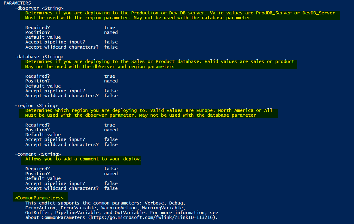
get-help .\Conflicting_Parameters_Help2.ps1 -Full

You will now see all your parameter help in its full glory! I’ve only reproduced the relevant part here with details highlighted

Note that the details about the parameters are now part of the help. You will also note that common parameters are also listed.

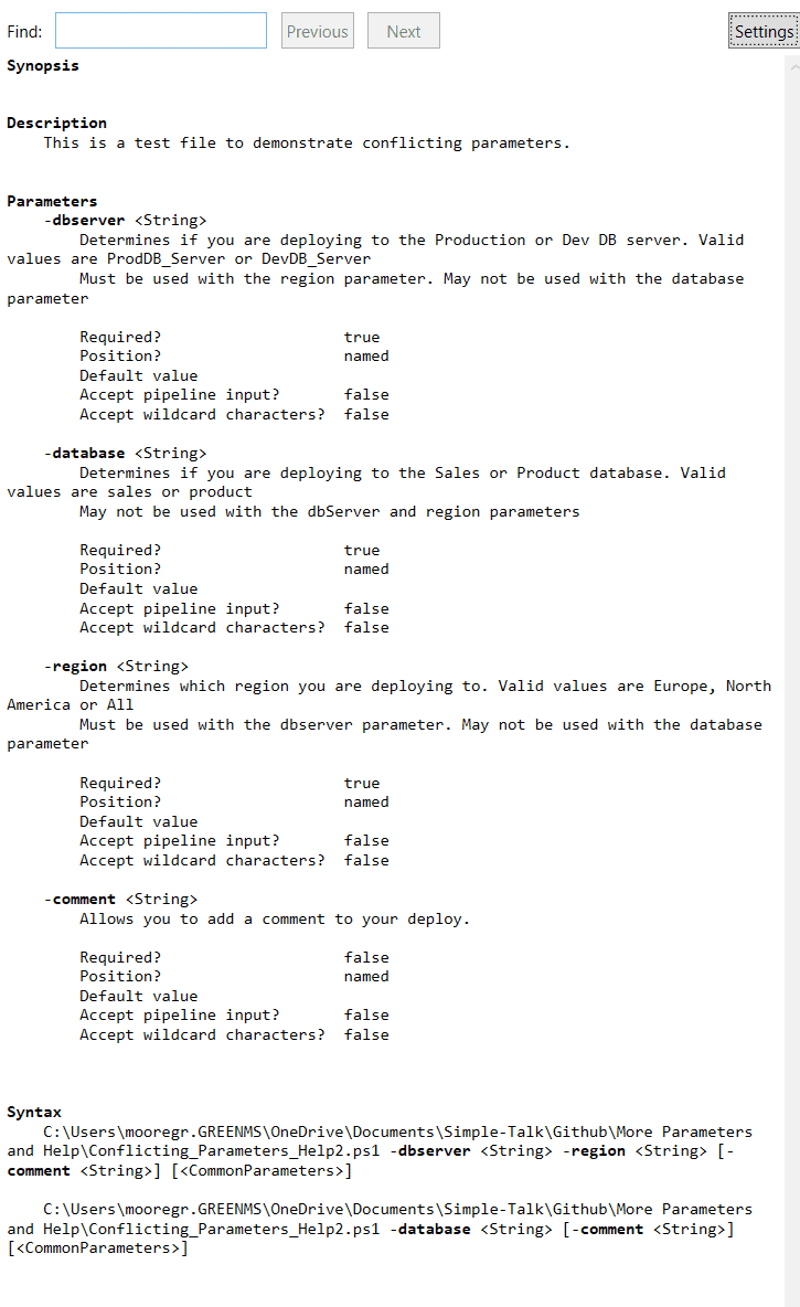
While this help text is useful, you may find yourself wanting it in a separate window so you can consult it while continue writing your script. In this case, try the following:

get-help .\Conflicting_Parameters_Help2.ps1 -showwindow

You should see a window similar to this:

Note that the examples nicely highlight the parameters and because there are two Parameter Sets, shows you both possibilities.

However, you may ask yourself, what if you want help on just one parameter? PowerShell allows for that also:

Run this code:

get-help .\Conflicting_Parameters_Help2.ps1 -Parameter dbserver

You should get:

You will also notice, in addition to the help details you’ve provided, PowerShell is also informing the user if the parameter is required, if it is handled by position and other details. In an earlier article, I discussed the value of naming parameters. I will cover pipeline input at a later date.

If you want to make life even easier for your users, you may want to include examples of how to execute the script with the proper parameters.

Add the following lines (again, remembering to have a blank line before and after the new lines) and save as Conflicting_Parameters_Help3.ps1.

.EXAMPLE
PS> .\Conflicting_Parameters_Help3 -dbserver ProdDB_Server -region 'North America' -Comment 'deployment by server and region example!'
.EXAMPLE
PS> .\Conflicting_Parameters_Help3 -database Sales -Comment 'deployment by database example!'
.SYNOPSIS
Used to determine where files should be deployed.


Then run the following:

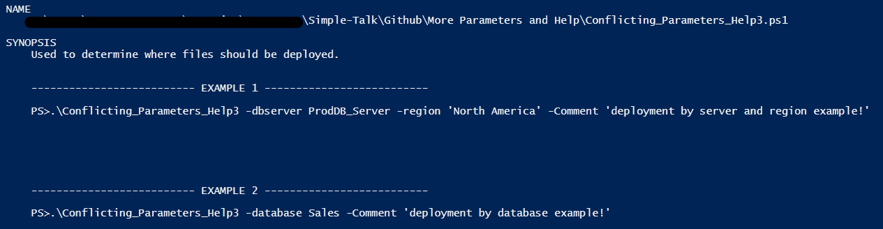
get-help .\Conflicting_Parameters_Help3.ps1 -Examples

You will get back something very much like:

If you cut and paste either example, it will run the command as expected. For example, using the first example will return:

Finally, I want to show you another way of adding help. It’s not one I would generally recommend but in some cases may be quicker and easier. For ease of coding, I’ll put the entire script here. It’s basically the last script with two minor modifications. Save it as Conflicting_Parameters_Help4.ps1.

<#
.Description
This is a test file to demonstrate conflicting parameters.
.PARAMETER database
Determines if you are deploying to the Sales or Product database. Valid values are sales or product
May not be used with the dbServer and region parameters
.PARAMETER region
Determines which region you are deploying to. Valid values are Europe, North America or All
Must be used with the dbserver parameter. May not be used with the database parameter
.PARAMETER Comment
Allows you to add a comment to your deploy.
.EXAMPLE
PS> .\Conflicting_Parameters_Help3 -dbserver ProdDB_Server -region 'North America' -Comment 'deployment by server and region example!'
.EXAMPLE
PS> .\Conflicting_Parameters_Help3 -database Sales -Comment 'deployment by database example!'
.SYNOPSIS
Used to determine where files should be deployed.
#>
param([parameter(mandatory, ParameterSetName='ByEnvironment')] [validateset("ProdDB_Server","DevDB_Server")] # Determines if you are deploying to the Production or Dev DB server. Valid values are ProdDB_Server or DevDB_Server Must be used with the region parameter. May not be used with the database parameter 
[string] $dbserver, 
[parameter(mandatory, ParameterSetName='ByDatabase')] [validateset("sales","product")] [string] $database, 
[parameter(mandatory, ParameterSetName='ByEnvironment')] [validateset("Europe","North America","All")] [string] $region,
[string] $comment) 
if ($dbserver)
{    
    Write-Host "Your code will be deployed to the $dbserver server in the $region region."
}
if ($database)
{
    Write-Host "Your code will be deployed to the $database database"
}
if ($comment)
{
    Write-host "Your comment was: $comment"
}


What you will notice is that I’ve removed the .PARAMETER help message for dbserver and moved it directly into the parameter definition.

As above, run this:

get-help .\Conflicting_Parameters_Help4.ps1 -Parameter dbserver

You should get:

The advantage of writing parameter help this way is that the help can be entered as you’re creating the parameter. However, I find it a bit harder to read this way. There’s also an additional issue. If you take Conflicting_Parameters_Help4.ps1 and add the following lines to the help comment and save it as Conflicting_Parameters_Help5.ps1.

.PARAMETER dbserver
Help here overrides what's in the parameter definition.

Then run it.

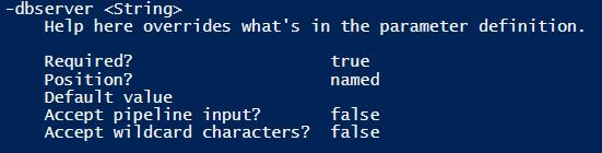
get-help .\Conflicting_Parameters_Help5.ps1 -Parameter dbserver

You will get:

While it can be handy to add the help message directly to the parameter definition, if you later go back and add a full comment-based help block, that will take precedence.

For the details on what you can add to your help block, I would recommend you read the Microsoft help for full details located here.

Conclusion

Hopefully, this article has helped you understand how to switch to better parameters and how to enable your users by adding a real PowerShell help to your scripts. As always, the scripts are available on GitHub.

The post How to Add Help to PowerShell Scripts appeared first on Simple Talk.


from Simple Talk https://ift.tt/2Wutmem
via

Wednesday, May 13, 2020

Database Kill and Fill

When testing database code in development, you usually have a lot of tests that aim to prove that the various processes such as ETL, reporting or the processing of an order, still work as they always did. If it is a changed process, you need to ensure that, from a known dataset, the process yields the result that the business expects. These tests happen as part of both development and deployment.

These datasets are generally created for each release and maintained to keep in step with the current development, being saved on the local filesystem as native BCP files. Sometimes, all or part of the live data is used, pseudonymised or masked where necessary. It is also handy to generate data, especially when you need large datasets to check that the database can scale appropriately.

Copying a database using a BCP dataset from a DOS script or from PowerShell is fairly quick and trivial, but what if the data is already in another copy of the database on the same instance? Imagine you have a database build that is a copy of an existing database on the same instance and you want to run a ‘destructive’ test on the data, and do it over and over again.

Deleting all the data in a database should, you’d have thought, be trivial. Truncation doesn’t work because it doesn’t like to truncate tables with foreign keys, even if they are disabled. DELETE is safer but you will need to then reset any identity columns. Deleting large tables in one chunk isn’t scalable, so you have to do it in smaller chunks. I like to disable triggers while I do this as well. The only disadvantage comes if you have triggers that are supposed to be disabled because the simple code just re-enables them all.

Killing data

Basically, if you are prepared to use sp_MSforeachtable, then this code is all reasonably simple. This will delete all the data from Adventureworks in about half a minute. It does Pubs in a second! Don’t use it without due care! This code is dangerous in untutored hands. You can try it out within a transaction and roll it back while you are testing.

---firstly delete all existing data
DISABLE TRIGGER ALL ON DATABASE;
--now disable all constraints
EXEC sp_MSforeachtable 'ALTER TABLE ? NOCHECK CONSTRAINT ALL';
--delete the data from each table in turn, doing tables with more than 10,000 rows in chuncks
EXEC sp_MSforeachtable '
Print ''Deleting all the data from ?''
SET QUOTED_IDENTIFIER ON;
DECLARE @SoFarDeleted INT=1;
WHILE (@SoFarDeleted  > 0 and @@Error=0)
  BEGIN
   -- Delete a chunk of rows at a time
     DELETE TOP (10000) ?
   SET @SoFarDeleted  = @@ROWCOUNT;
END ';
--switch on all constraints
EXEC sp_MSforeachtable 'ALTER TABLE ? WITH CHECK CHECK CONSTRAINT ALL';
-- Reseed identity columns if the table has an identity column
EXEC sp_MSforeachtable 'IF ObjectPropertyEx(Object_Id(''?''),''TableHasIdentity'')=1 DBCC CHECKIDENT (''?'', RESEED, 0)';
-- and enable all triggers
ENABLE TRIGGER ALL ON DATABASE;


Filling data

Now to get that data back in. you have a copy of the database on the same server so you use that. All you need to do, surely is to …

INSERT INTO tableA SELECT * FROM otherDatabase.tableA;

… for all the tables in the database? No. For a start, you cannot insert into a timestamp column, and you need to SET IDENTITY INSERT TableA ON in order to insert into TableA, which has an identity column. If course, if you try this with a table that hasn’t an identity column you get an error. Inserting XML into an XML column results in an error unless you do an explicit conversion (because of the possibility of a different XML Schema). You have to ignore calculated columns as well. You can’t insert into a calculated column or a timestamp column. I have no idea whether it is possible or desirable to insert into a hidden column so I disallowed that too. Change it to taste.

Out of the box, this code doesn’t work on older versions of SQL Server because I use the lovely string_agg function to generate lists of columns. You can change this to the classic XML trick to get the same result if you are stuck on an old version. Anything older than SQL Server 2016 didn’t have the is_hidden attribute in the sys.columns system view

Here, I have it set, for the sake of demonstration, to delete all the data from a database called AdventureworksCopy, and fill it again from Adventureworks2016. You’ll want to change that!

USE AdventureworksCopy;
GO
DECLARE @source sysname = 'Adventureworks2016';-- the source of the database

---firstly delete all existing data
DISABLE TRIGGER ALL ON DATABASE;
--now disable all constraints
EXEC sp_MSforeachtable 'ALTER TABLE ? NOCHECK CONSTRAINT ALL';
--delete the data from each table in turn, doing tables with more than 10,000 rows in chuncks
EXEC sp_MSforeachtable '
Print ''Deleting all the data from ?''
SET QUOTED_IDENTIFIER ON;
DECLARE @SoFarDeleted INT=1;
WHILE (@SoFarDeleted  > 0 and @@Error=0)
  BEGIN
   -- Delete a chunk of rows at a time
     DELETE TOP (10000) ?
   SET @SoFarDeleted  = @@ROWCOUNT;
END ';
--switch on all constraints
EXEC sp_MSforeachtable 'ALTER TABLE ? WITH CHECK CHECK CONSTRAINT ALL';
-- Reseed identity columns if the table has an identity column
EXEC sp_MSforeachtable 'IF ObjectPropertyEx(Object_Id(''?''),''TableHasIdentity'')=1 DBCC CHECKIDENT (''?'', RESEED, 0)';
-- and enable all triggers
ENABLE TRIGGER ALL ON DATABASE;
--create a table variable giving all the table names so we can do each one
DECLARE @tables TABLE
  (
  TableName_id INT IDENTITY,
  TheObject_ID INT NOT NULL,
  TheName sysname NOT NULL,
  TheSchema sysname NOT NULL
  );
--fill the table with the names of the tables we need to fill
INSERT INTO @tables (TheObject_ID, TheName, TheSchema)
  SELECT object_id, name, Object_Schema_Name(object_id) FROM sys.tables;
--and to prevent a generated script getting too untidy ---
DECLARE @CRLF CHAR(2) = '
';
--      We disable all constraints now   
DECLARE @Script NVARCHAR(MAX) =
  'EXEC sp_msforeachtable "ALTER TABLE ? NOCHECK CONSTRAINT ALL"' + @CRLF;
DECLARE @ii INT, @iiMax INT; ---our iteration counter
DECLARE @TheTableName sysname, @TheSelectColumns NVARCHAR(MAX),
  @TheInsertColumns NVARCHAR(MAX), @TheTable_id INT, @HasIdentityCol INT;
--set our iteration counters
SELECT @ii = Min(TableName_id), @iiMax = Max(TableName_id) FROM @tables;
--we need to have a table with all the source tables in it just in case we
--have an extra table in the destination with no equivalent in the source
DECLARE @sourceTables TABLE (TableName sysname);
DECLARE @Expression NVARCHAR(MAX) = --the expression we execute
  N'USE ' + @source
  + ' SELECT QuoteName(Object_Schema_Name(t.object_id)) + ''.'' + QuoteName(t.name)  FROM sys.tables t';
--and get the list of the tables in the other database
INSERT INTO @sourceTables EXECUTE (@Expression);
--now we can get cracking and generate a script that fills each table in turn
WHILE @ii <= @iiMax
  BEGIN
    SELECT @TheTable_id = TheObject_ID,
      @TheTableName = QuoteName(TheSchema) + '.' + QuoteName(TheName)
      FROM @tables
      WHERE TableName_id = @ii; --get the table name
    SELECT @ii = @ii + 1; --don't fill it if it isn't in the source
    IF @TheTableName NOT IN (SELECT TableName FROM @sourceTables) CONTINUE;
    SELECT @TheInsertColumns = --get the list of columns in the insert expression
      String_Agg(QuoteName(columns.name), ', ') WITHIN GROUP(
      ORDER BY column_id ASC),
      @TheSelectColumns =--get the list of columns in the select expression
        String_Agg( CASE WHEN types.name = 'xml'  --convert XML types 
                                        THEN 'Convert(XML, ' + QuoteName(columns.name) + ')' 
                                        ELSE QuoteName(columns.name) END,
                    ', '
                  ) WITHIN GROUP(ORDER BY column_id ASC)
      FROM sys.columns
        INNER JOIN sys.types
          ON types.user_type_id = COLUMNS.user_type_id
      WHERE object_id = @TheTable_id
        AND is_hidden = 0 --don't use hidden columns
        AND is_computed = 0--don't use computed columns either
        AND types.name NOT LIKE 'timestamp';--don't use timestamp columns
    SELECT @HasIdentityCol =Convert(INT,ObjectPropertyEx(@TheTable_id ,'TableHasIdentity'))
    SELECT @Script =
      @Script
      + CASE WHEN @HasIdentityCol > 0 THEN /*IF there is an identity column we 
          need to set identity insert on for the table */
               'SET IDENTITY_INSERT ' + @TheTableName + ' ON  ' ELSE '' END
      + @CRLF + N'Print ''Adding data to table ' + @TheTableName + N' '''
      + @CRLF + N'INSERT INTO ' + @TheTableName + N'(' + @TheInsertColumns
      + N') ' + @CRLF + N'SELECT ' + @TheSelectColumns + N' FROM ' + @source
      + N'.' + @TheTableName + @CRLF
      + CASE WHEN @HasIdentityCol > 0 THEN /*IF there is an identity column we 
          switched identity insert on so we need to switch it off */
               'SET IDENTITY_INSERT ' + @TheTableName + ' OFF' + @CRLF ELSE '' END
      + @CRLF;
  END;
SELECT @Script =
  @Script
  + '
  EXEC sp_msforeachtable "ALTER TABLE ? WITH CHECK CHECK CONSTRAINT ALL"';

EXECUTE (@Script);
GO

Conclusions

Am I recommending Kill and Fill? It depends on what sort of testing you are doing. A BCP process is always nice, quick and clean, though it still needs the kill part of the process, but it is best done from a Dos shell script or a PowerShell script. This Kill and Fill process is easy to set up though I don’t think it is any quicker than a bulk process. I just thought I should make it available just in case anyone else needed a different way of filling a development database with data.

The post Database Kill and Fill appeared first on Simple Talk.


from Simple Talk https://ift.tt/3buySSk
via
Text Mining and Sentiment Analysis: Analysis with R

The series so far:

  1. Text Mining and Sentiment Analysis: Introduction
  2. Text Mining and Sentiment Analysis: Power BI Visualizations
  3. Text Mining and Sentiment Analysis: Analysis with R

This is the third article of the “Text Mining and Sentiment Analysis” Series. The first article introduced Azure Cognitive Services and demonstrated the setup and use of Text Analytics APIs for extracting key Phrases & Sentiment Scores from text data. The second article demonstrated Power BI visualizations for analyzing Key Phrases & Sentiment Scores and interpreting them to gain insights. This article explores R for text mining and sentiment analysis. I will demonstrate several common text analytics techniques and visualizations in R.

Note: This article assumes basic familiarity with R and RStudio. Please jump to the References section for more information on installing R and RStudio. The Demo data raw text file and R script are available for download from my GitHub repository; please find the link in the References section.
R is a language and environment for statistical computing and graphics. It provides a wide variety of statistical and graphical techniques and is highly extensible. R is available as free software. It’s easy to learn

and use and can produce well designed publication-quality plots. For the demos in this article, I am using R version 3.5.3 (2019-03-11), RStudio Version 1.1.456

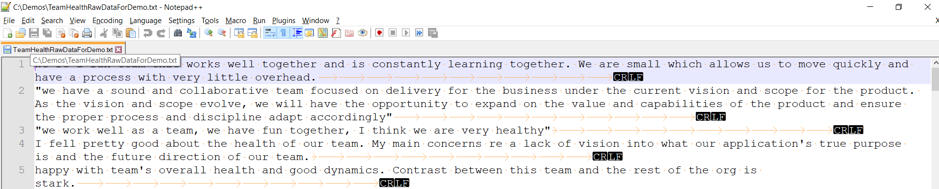
The input file for this article has only one column, the “Raw text” of survey responses and is a text file.

A sample of the first few rows are shown in Notepad++ (showing all characters) in Figure 1.

A screenshot of a computer Description automatically generated

Figure 1. Sample of the input text file

The demo R script and demo input text file are available on my GitHub repo (please find the link in the References section).

R has a rich set of packages for Natural Language Processing (NLP) and generating plots. The foundational steps involve loading the text file into an R Corpus, then cleaning and stemming the data before performing analysis. I will demonstrate these steps and analysis like Word Frequency, Word Cloud, Word Association, Sentiment Scores and Emotion Classification using various plots and charts.

Installing and loading R packages

The following packages are used in the examples in this article:

  • tm for text mining operations like removing numbers, special characters, punctuations and stop words (Stop words in any language are the most commonly occurring words that have very little value for NLP and should be filtered out. Examples of stop words in English are “the”, “is”, “are”.)
  • snowballc for stemming, which is the process of reducing words to their base or root form. For example, a stemming algorithm would reduce the words “fishing”, “fished” and “fisher” to the stem “fish”.
  • wordcloud for generating the word cloud plot.
  • RColorBrewer for color palettes used in various plots
  • syuzhet for sentiment scores and emotion classification
  • ggplot2 for plotting graphs

Open RStudio and create a new R Script. Use the following code to install and load these packages.

# Install
install.packages("tm")  # for text mining
install.packages("SnowballC") # for text stemming
install.packages("wordcloud") # word-cloud generator 
install.packages("RColorBrewer") # color palettes
install.packages("syuzhet") # for sentiment analysis
install.packages("ggplot2") # for plotting graphs
# Load
library("tm")
library("SnowballC")
library("wordcloud")
library("RColorBrewer")
library("syuzhet")
library("ggplot2")

Reading file data into R

The R base function read.table() is generally used to read a file in table format and imports data as a data frame. Several variants of this function are available, for importing different file formats;

  • read.csv() is used for reading comma-separated value (csv) files, where a comma “,” is used a field separator
  • read.delim() is used for reading tab-separated values (.txt) files

The input file has multiple lines of text and no columns/fields (data is not tabular), so you will use the readLines function. This function takes a file (or URL) as input and returns a vector containing as many elements as the number of lines in the file. The readLines function simply extracts the text from its input source and returns each line as a character string. The n= argument is useful to read a limited number (subset) of lines from the input source (Its default value is -1, which reads all lines from the input source). When using the filename in this function’s argument, R assumes the file is in your current working directory (you can use the getwd() function in R console to find your current working directory). You can also choose the input file interactively, using the file.choose() function within the argument. The next step is to load that Vector as a Corpus. In R, a Corpus is a collection of text document(s) to apply text mining or NLP routines on. Details of using the readLines function are sourced from: https://www.stat.berkeley.edu/~spector/s133/Read.html .

In your R script, add the following code to load the data into a corpus.

# Read the text file from local machine , choose file interactively
text <- readLines(file.choose())
# Load the data as a corpus
TextDoc <- Corpus(VectorSource(text))

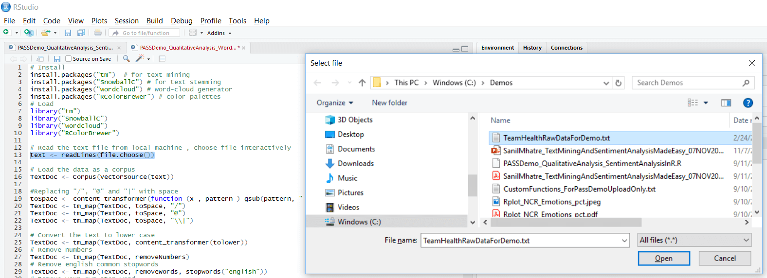
Upon running this, you will be prompted to select the input file. Navigate to your file and click Open as shown in Figure 2.

A screenshot of a computer Description automatically generated

Figure 2. Select input file

Cleaning up Text Data

Cleaning the text data starts with making transformations like removing special characters from the text. This is done using the tm_map() function to replace special characters like /, @ and | with a space. The next step is to remove the unnecessary whitespace and convert the text to lower case.

Then remove the stopwords. They are the most commonly occurring words in a language and have very little value in terms of gaining useful information. They should be removed before performing further analysis. Examples of stopwords in English are “the, is, at, on. There is no single universal list of stop words used by all NLP tools. stopwords in the tm_map() function supports several languages like English, French, German, Italian, and Spanish. Please note the language names are case sensitive. I will also demonstrate how to add your own list of stopwords, which is useful in this Team Health example for removing non-default stop words like “team”, “company”, “health”. Next, remove numbers and punctuation.

The last step is text stemming. It is the process of reducing the word to its root form. The stemming process simplifies the word to its common origin. For example, the stemming process reduces the words “fishing”, “fished” and “fisher” to its stem “fish”. Please note stemming uses the SnowballC package. (You may want to skip the text stemming step if your users indicate a preference to see the original “unstemmed” words in the word cloud plot)

In your R script, add the following code to transform and run to clean-up the text data.

#Replacing "/", "@" and "|" with space
toSpace <- content_transformer(function (x , pattern ) gsub(pattern, " ", x))
TextDoc <- tm_map(TextDoc, toSpace, "/")
TextDoc <- tm_map(TextDoc, toSpace, "@")
TextDoc <- tm_map(TextDoc, toSpace, "\\|")
# Convert the text to lower case
TextDoc <- tm_map(TextDoc, content_transformer(tolower))
# Remove numbers
TextDoc <- tm_map(TextDoc, removeNumbers)
# Remove english common stopwords
TextDoc <- tm_map(TextDoc, removeWords, stopwords("english"))
# Remove your own stop word
# specify your custom stopwords as a character vector
TextDoc <- tm_map(TextDoc, removeWords, c("s", "company", "team")) 
# Remove punctuations
TextDoc <- tm_map(TextDoc, removePunctuation)
# Eliminate extra white spaces
TextDoc <- tm_map(TextDoc, stripWhitespace)
# Text stemming - which reduces words to their root form
TextDoc <- tm_map(TextDoc, stemDocument)


Building the term document matrix

After cleaning the text data, the next step is to count the occurrence of each word, to identify popular or trending topics. Using the function TermDocumentMatrix() from the text mining package, you can build a Document Matrix – a table containing the frequency of words.

In your R script, add the following code and run it to see the top 5 most frequently found words in your text.

# Build a term-document matrix
TextDoc_dtm <- TermDocumentMatrix(TextDoc)
dtm_m <- as.matrix(TextDoc_dtm)
# Sort by descearing value of frequency
dtm_v <- sort(rowSums(dtm_m),decreasing=TRUE)
dtm_d <- data.frame(word = names(dtm_v),freq=dtm_v)
# Display the top 5 most frequent words
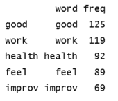
head(dtm_d, 5)

The following table of word frequency is the expected output of the head command on RStudio Console.


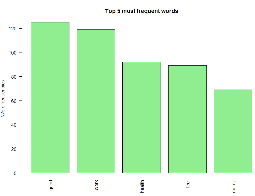
Plotting the top 5 most frequent words using a bar chart is a good basic way to visualize this word frequent data. In your R script, add the following code and run it to generate a bar chart, which will display in the Plots sections of RStudio.

# Plot the most frequent words
barplot(dtm_d[1:5,]$freq, las = 2, names.arg = dtm_d[1:5,]$word,
        col ="lightgreen", main ="Top 5 most frequent words",
        ylab = "Word frequencies")

The plot can be seen in Figure 3.

A screenshot of a cell phone Description automatically generated

Figure 3. Bar chart of the top 5 most frequent words

One could interpret the following from this bar chart:

  • The most frequently occurring word is “good”. Also notice that negative words like “not” don’t feature in the bar chart, which indicates there are no negative prefixes to change the context or meaning of the word “good” ( In short, this indicates most responses don’t mention negative phrases like “not good”).
  • “work”, “health” and “feel” are the next three most frequently occurring words, which indicate that most people feel good about their work and their team’s health.
  • Finally, the root “improv” for words like “improve”, “improvement”, “improving”, etc. is also on the chart, and you need further analysis to infer if its context is positive or negative

Generate the Word Cloud

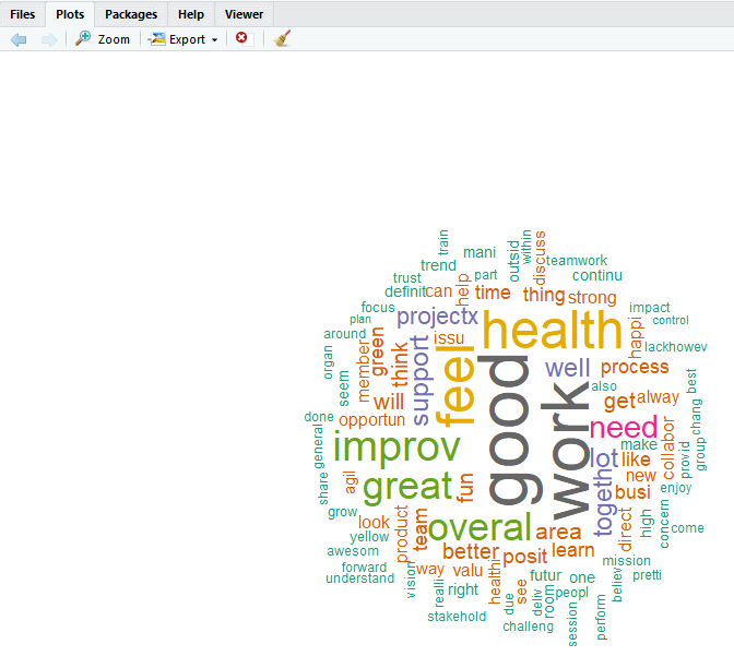
A word cloud is one of the most popular ways to visualize and analyze qualitative data. It’s an image composed of keywords found within a body of text, where the size of each word indicates its frequency in that body of text. Use the word frequency data frame (table) created previously to generate the word cloud. In your R script, add the following code and run it to generate the word cloud and display it in the Plots section of RStudio.

#generate word cloud
set.seed(1234)
wordcloud(words = dtm_d$word, freq = dtm_d$freq, min.freq = 5,
          max.words=100, random.order=FALSE, rot.per=0.40, 
          colors=brewer.pal(8, "Dark2"))

Below is a brief description of the arguments used in the word cloud function;

  • words – words to be plotted
  • freq – frequencies of words
  • min.freq – words whose frequency is at or above this threshold value is plotted (in this case, I have set it to 5)
  • max.words – the maximum number of words to display on the plot (in the code above, I have set it 100)
  • random.order – I have set it to FALSE, so the words are plotted in order of decreasing frequency
  • rot.per – the percentage of words that are displayed as vertical text (with 90-degree rotation). I have set it 0.40 (40 %), please feel free to adjust this setting to suit your preferences
  • colors – changes word colors going from lowest to highest frequencies

You can see the resulting word cloud in Figure 4.

A screenshot of a cell phone Description automatically generated

Figure 4. Word cloud plot

The word cloud shows additional words that occur frequently and could be of interest for further analysis. Words like “need”, “support”, “issu” (root for “issue(s)”, etc. could provide more context around the most frequently occurring words and help to gain a better understanding of the main themes.

Word Association

Correlation is a statistical technique that can demonstrate whether, and how strongly, pairs of variables are related. This technique can be used effectively to analyze which words occur most often in association with the most frequently occurring words in the survey responses, which helps to see the context around these words

In your R script, add the following code and run it.

# Find associations 
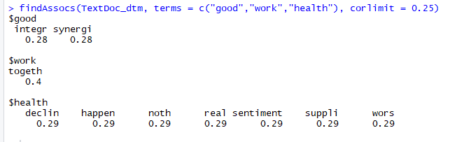
findAssocs(TextDoc_dtm, terms = c("good","work","health"), corlimit = 0.25)

You should see the results as shown in Figure 5.

A screenshot of a cell phone Description automatically generated

Figure 5. Word association analysis for the top three most frequent terms

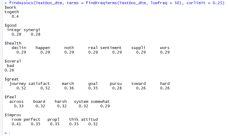
This script shows which words are most frequently associated with the top three terms (corlimit = 0.25 is the lower limit/threshold I have set. You can set it lower to see more words, or higher to see less). The output indicates that “integr” (which is the root for word “integrity”) and “synergi” (which is the root for words “synergy”, “synergies”, etc.) and occur 28% of the time with the word “good”. You can interpret this as the context around the most frequently occurring word (“good”) is positive. Similarly, the root of the word “together” is highly correlated with the word “work”. This indicates that most responses are saying that teams “work together” and can be interpreted in a positive context.

You can modify the above script to find terms associated with words that occur at least 50 times or more, instead of having to hard code the terms in your script.

# Find associations for words that occur at least 50 times
findAssocs(TextDoc_dtm, terms = findFreqTerms(TextDoc_dtm, lowfreq = 50), corlimit = 0.25)

A screenshot of a cell phone Description automatically generated

Figure 6: Word association output for terms occurring at least 50 times

Sentiment Scores

Sentiments can be classified as positive, neutral or negative. They can also be represented on a numeric scale, to better express the degree of positive or negative strength of the sentiment contained in a body of text.

This example uses the Syuzhet package for generating sentiment scores, which has four sentiment dictionaries and offers a method for accessing the sentiment extraction tool developed in the NLP group at Stanford. The get_sentiment function accepts two arguments: a character vector (of sentences or words) and a method. The selected method determines which of the four available sentiment extraction methods will be used. The four methods are syuzhet (this is the default), bing, afinn and nrc. Each method uses a different scale and hence returns slightly different results. Please note the outcome of nrc method is more than just a numeric score, requires additional interpretations and is out of scope for this article. The descriptions of the get_sentiment function has been sourced from : https://cran.r-project.org/web/packages/syuzhet/vignettes/syuzhet-vignette.html?

Add the following code to the R script and run it.

# regular sentiment score using get_sentiment() function and method of your choice
# please note that different methods may have different scales
syuzhet_vector <- get_sentiment(text, method="syuzhet")
# see the first row of the vector
head(syuzhet_vector)
# see summary statistics of the vector
summary(syuzhet_vector)

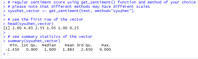
Your results should look similar to Figure 7.

A screenshot of a cell phone Description automatically generated

Figure 7. Syuzhet vector

An inspection of the Syuzhet vector shows the first element has the value of 2.60. It means the sum of the sentiment scores of all meaningful words in the first response(line) in the text file, adds up to 2.60. The scale for sentiment scores using the syuzhet method is decimal and ranges from -1(indicating most negative) to +1(indicating most positive). Note that the summary statistics of the suyzhet vector show a median value of 1.6, which is above zero and can be interpreted as the overall average sentiment across all the responses is positive.

Next, run the same analysis for the remaining two methods and inspect their respective vectors. Add the following code to the R script and run it.

# bing
bing_vector <- get_sentiment(text, method="bing")
head(bing_vector)
summary(bing_vector)
#affin
afinn_vector <- get_sentiment(text, method="afinn")
head(afinn_vector)
summary(afinn_vector)

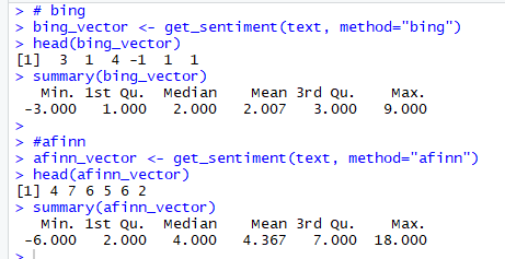
Your results should resemble Figure 8.

A screenshot of a cell phone Description automatically generated

Figure 8. bing and afinn vectors

Please note the scale of sentiment scores generated by:

  • bing – binary scale with -1 indicating negative and +1 indicating positive sentiment
  • afinn – integer scale ranging from -5 to +5

The summary statistics of bing and afinn vectors also show that the Median value of Sentiment scores is above 0 and can be interpreted as the overall average sentiment across the all the responses is positive.

Because these different methods use different scales, it’s better to convert their output to a common scale before comparing them. This basic scale conversion can be done easily using R’s built-in sign function, which converts all positive number to 1, all negative numbers to -1 and all zeros remain 0.

Add the following code to your R script and run it.

#compare the first row of each vector using sign function
rbind(
  sign(head(syuzhet_vector)),
  sign(head(bing_vector)),
  sign(head(afinn_vector))
)

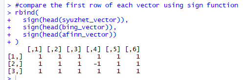
Figure 9 shows the results.

A screenshot of a cell phone Description automatically generated

Figure 9. Normalize scale and compare three vectors

Note the first element of each row (vector) is 1, indicating that all three methods have calculated a positive sentiment score, for the first response (line) in the text.

Emotion Classification

Emotion classification is built on the NRC Word-Emotion Association Lexicon (aka EmoLex). The definition of “NRC Emotion Lexicon”, sourced from http://saifmohammad.com/WebPages/NRC-Emotion-Lexicon.htm is “The NRC Emotion Lexicon is a list of English words and their associations with eight basic emotions (anger, fear, anticipation, trust, surprise, sadness, joy, and disgust) and two sentiments (negative and positive). The annotations were manually done by crowdsourcing.”

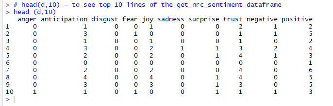
To understand this, explore the get_nrc_sentiments function, which returns a data frame with each row representing a sentence from the original file. The data frame has ten columns (one column for each of the eight emotions, one column for positive sentiment valence and one for negative sentiment valence). The data in the columns (anger, anticipation, disgust, fear, joy, sadness, surprise, trust, negative, positive) can be accessed individually or in sets. The definition of get_nrc_sentiments has been sourced from: https://cran.r-project.org/web/packages/syuzhet/vignettes/syuzhet-vignette.html?

Add the following line to your R script and run it, to see the data frame generated from the previous execution of the get_nrc_sentiment function.

# run nrc sentiment analysis to return data frame with each row classified as one of the following
# emotions, rather than a score: 
# anger, anticipation, disgust, fear, joy, sadness, surprise, trust 
# It also counts the number of positive and negative emotions found in each row
d<-get_nrc_sentiment(text)
# head(d,10) - to see top 10 lines of the get_nrc_sentiment dataframe
head (d,10)

The results should look like Figure 10.

A screenshot of a cell phone Description automatically generated

Figure 10. Data frame returned by get_nrc_sentiment function

The output shows that the first line of text has;

  • Zero occurrences of words associated with emotions of anger, disgust, fear, sadness and surprise
  • One occurrence each of words associated with emotions of anticipation and joy
  • Two occurrences of words associated with emotions of trust
  • Total of one occurrence of words associated with negative emotions
  • Total of two occurrences of words associated with positive emotions

The next step is to create two plots charts to help visually analyze the emotions in this survey text. First, perform some data transformation and clean-up steps before plotting charts. The first plot shows the total number of instances of words in the text, associated with each of the eight emotions. Add the following code to your R script and run it.

#transpose
td<-data.frame(t(d))
#The function rowSums computes column sums across rows for each level of a grouping variable.
td_new <- data.frame(rowSums(td[2:253]))
#Transformation and cleaning
names(td_new)[1] <- "count"
td_new <- cbind("sentiment" = rownames(td_new), td_new)
rownames(td_new) <- NULL
td_new2<-td_new[1:8,]
#Plot One - count of words associated with each sentiment
quickplot(sentiment, data=td_new2, weight=count, geom="bar", fill=sentiment, ylab="count")+ggtitle("Survey sentiments")

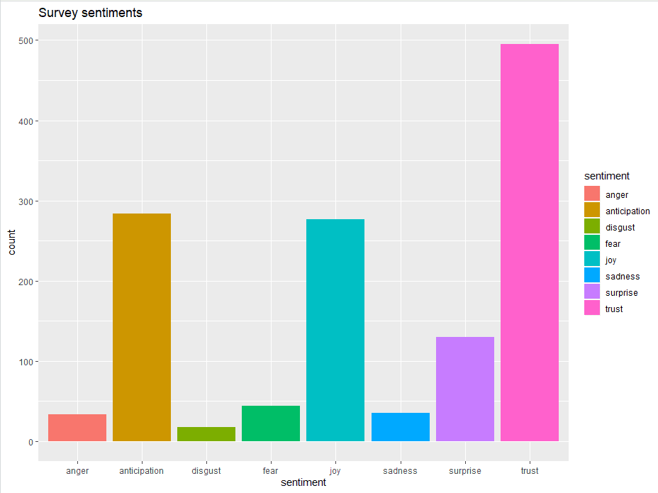
You can see the bar plot in Figure 11.

A screenshot of a cell phone Description automatically generated

Figure 11. Bar Plot showing the count of words in the text, associated with each emotion

This bar chart demonstrates that words associated with the positive emotion of “trust” occurred about five hundred times in the text, whereas words associated with the negative emotion of “disgust” occurred less than 25 times. A deeper understanding of the overall emotions occurring in the survey response can be gained by comparing these number as a percentage of the total number of meaningful words. Add the following code to your R script and run it.

#Plot two - count of words associated with each sentiment, expressed as a percentage
barplot(
  sort(colSums(prop.table(d[, 1:8]))), 
  horiz = TRUE, 
  cex.names = 0.7, 
  las = 1, 
  main = "Emotions in Text", xlab="Percentage"
)

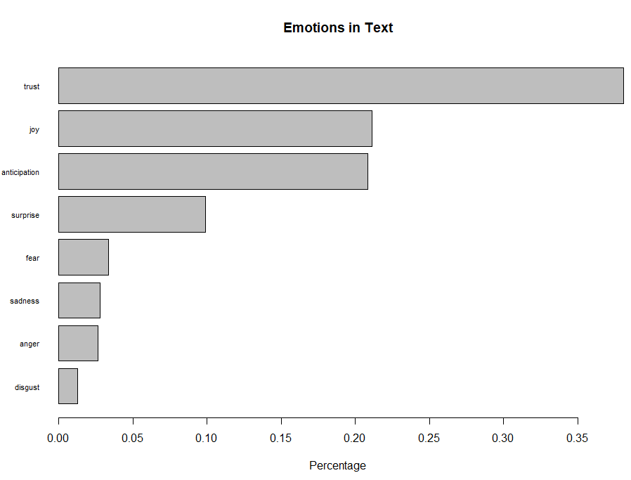
The Emotions bar plot can be seen in figure 12.

A screenshot of a cell phone Description automatically generated

Figure 12. Bar Plot showing the count of words associated with each sentiment expressed as a percentage

This bar plot allows for a quick and easy comparison of the proportion of words associated with each emotion in the text. The emotion “trust” has the longest bar and shows that words associated with this positive emotion constitute just over 35% of all the meaningful words in this text. On the other hand, the emotion of “disgust” has the shortest bar and shows that words associated with this negative emotion constitute less than 2% of all the meaningful words in this text. Overall, words associated with the positive emotions of “trust” and “joy” account for almost 60% of the meaningful words in the text, which can be interpreted as a good sign of team health.

Conclusion

This article demonstrated reading text data into R, data cleaning and transformations. It demonstrated how to create a word frequency table and plot a word cloud, to identify prominent themes occurring in the text. Word association analysis using correlation, helped gain context around the prominent themes. It explored four methods to generate sentiment scores, which proved useful in assigning a numeric value to strength (of positivity or negativity) of sentiments in the text and allowed interpreting that the average sentiment through the text is trending positive. Lastly, it demonstrated how to implement an emotion classification with NRC sentiment and created two plots to analyze and interpret emotions found in the text.

References:


The post Text Mining and Sentiment Analysis: Analysis with R appeared first on Simple Talk.


from Simple Talk https://ift.tt/2Lrr3Ta
via

Tuesday, May 12, 2020

How to Use Scriptable Objects in Unity

Suppose you’re making a role-playing video game and you need an easier way to assign statistics, properties, and much more to various items. While you could use Unity prefabs to do this and then change the values of each individual copy of the prefab, this is an inconvenient way to go about the task. For starters, this method uses up more of your memory, something you may need to conserve if you plan on making a large game. In addition, if you must make any changes to the in-game objects, it’s simply not as efficient to do so when there are several copies of prefabs lying around. This especially becomes an issue if you have a larger team to work with, so you’ll want to make things easier to change for other team members. Even if you’re not in a team, this method would just be harder on you as you work.

To make things easier in a situation like this, you have Scriptable Objects at your disposal. And what are Scriptable Objects? Simply put, they are data containers. The Unity developer creates a basic template for these containers, defining what information each object should contain. Then the Scriptable Objects are created from that template, which are then used by Unity game objects. In the above example, a single Scriptable Object can be used to define what the different properties of an item are. Then that Scriptable Object is referenced by all copies of the item. Before if you wanted to change an item’s stats, you’d have to change the values of every single copy of the item. Now with Scriptable Objects, you only need to change one object (the Scriptable Object) and all objects getting data from that Scriptable Object change at the same time.

It’s always helpful to see these things in action, create a new project. This project shows off Scriptable Objects and how they can help you. The project consists of three game objects meant to represent three characters. Each character inherits some values from a Scriptable Object. Those values are maximum health, attack, defense, speed, and a name and color for the character. A simple user interface displays these values so you can easily see the results of applying Scriptable Objects. Now that you have an end goal, it’s time to get creating.

Project Setup

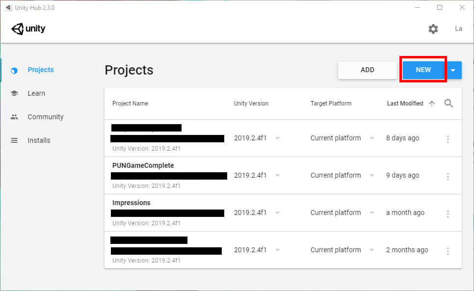
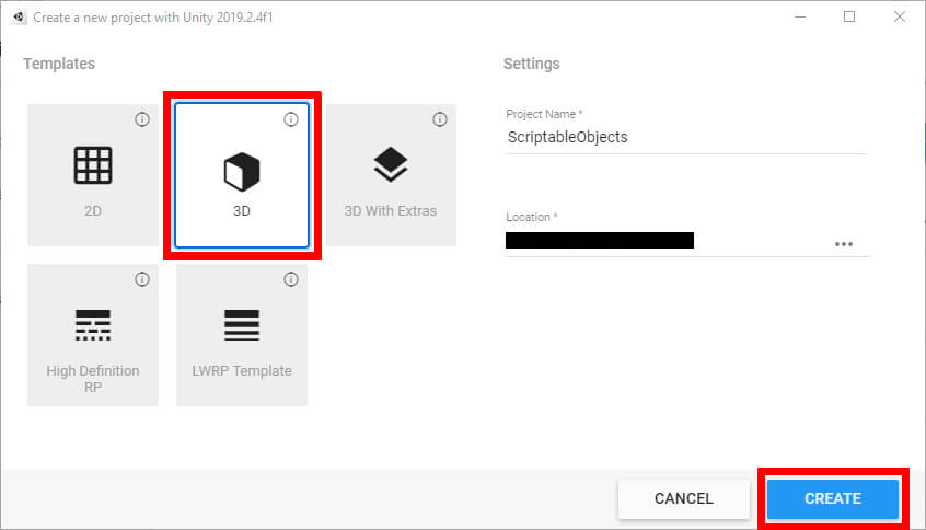
Assuming you’ll be implementing these ideas in a new project, open up the Unity Hub application and create a new project as shown in Figure 1.

Figure 1: Creating a new project

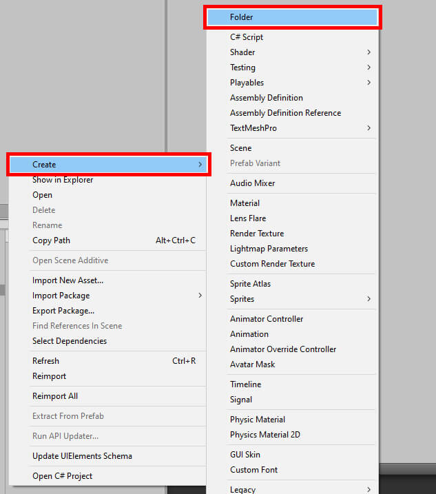
In the next window, give the project any name of your choosing and decide on the file path. While you can perform this project in any template, this example uses the 3D project template as shown in Figure 2. It’s recommended you use this template if you wish to follow along.

Figure 2: Setting the project name, type, and location

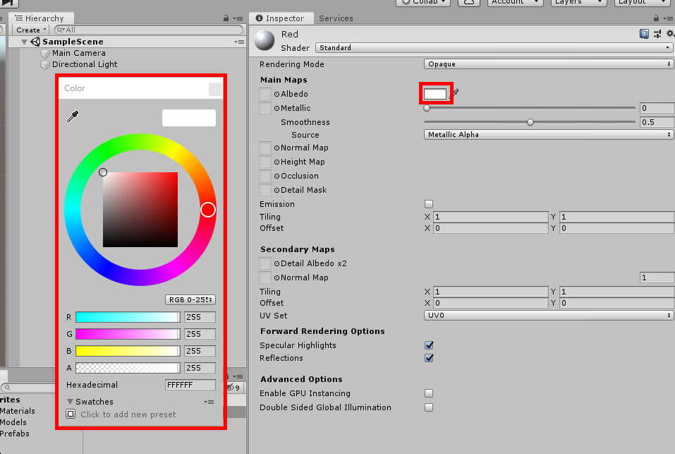
Once the project is created, you’ll want to get organized. In your Assets window, you’ll need to create three folders by right-clicking the window and navigating to Create -> Folder as shown in Figure 3 Name the folders Materials, Scriptable Objects, and Scripts.

Figure 3: Creating a new folder

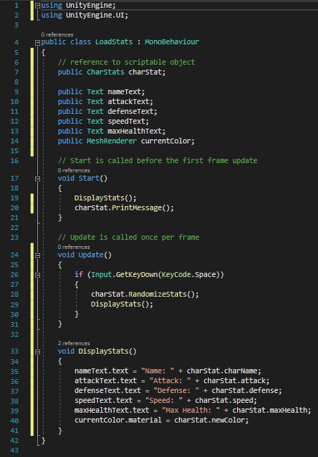
While you’re here, it’s a good idea to go ahead and get three materials made. These materials are used to change the colors of different objects following whatever material the Scriptable Object specifies. To create these materials, navigate to the Materials folder and right-click again, this time selecting Create -> Material. When naming the material, it’s recommended to give it a name that correlates with its color. For instance, this first material can be named Red. To set this color, you must select the newly created material and navigate to the Inspector window. In the Albedo field, there’s a color picker shown in Figure 4 you can click on to open the, well, color picker.

Figure 4: Opening the color picker

The color is changed either by moving the small circle in the color picker or by directly inputting the RGB values in the lower half of the color picker window. In the above example, the RGB values would be 255, 0, 0. After this, you should create two more materials and assign their colors. This example uses green and blue, but they can be any color of your choosing.

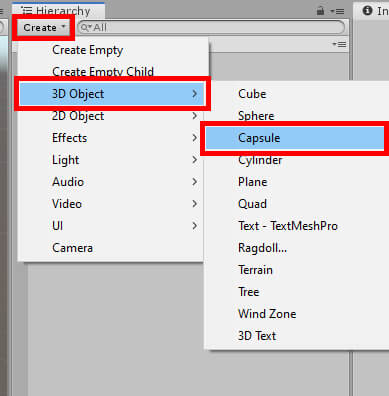
Now comes the time to create the actual scene this where this game takes place. It consists of two major parts – there’s the user interface which displays the statistics given to various scriptable objects and the three capsules representing characters. The “characters” are the easiest part, so you can start there. All you have to do is go to the Hierarchy window, click the Create button, and choose 3D Object -> Capsule shown in Figure 5. Do this three times or copy the first object, and you can also give them names if you wish. This example gives the capsules the names Char1, Char2, Char3.

Figure 5: Creating a capsule object

You’ll need to change their positions, so they aren’t overlapping each other. To change the object’s position, you select one in the Hierarchy and navigate to the Transform component in the Inspector. Then change the x, y, and z positioning fields to move the objects where you want them.

Figure 6: Editing the object’s position

Table 1 shows the exact positions of all three capsules in this example.

Table 1: All objects and their positions in the world

Object

X Position

Y Position

Z Position

Char1

-4

0

-5

Char2

0.5

0

-4

Char3

4

0

-5


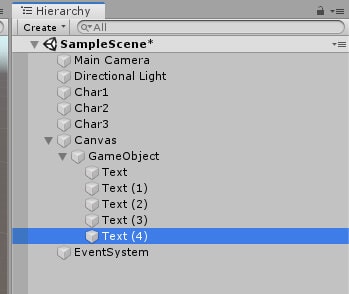
Of course, feel free to adjust any of these numbers if you wish. Next up is the user interface, which displays the values given to Scriptable Objects. To start, you’ll need to click the Hierarchy’s Create button but this time choose UI -> Canvas. Then, with the new Canvas object selected, click the Create button again and this time select Create Empty Child. Finally, once more you click the Create button and this time choose UI -> Text. Drag the newly created Text object onto the empty game object and duplicate Text four times using Ctrl + D so that there is a total of five Text objects under GameObject. Once finished, your Hierarchy should look like the one in Figure 7.

Figure 7: The current Hierarchy

Each Text object correlates to the name and stats that are given via Scriptable Object, those stats being maximum health, attack, defense, and speed. It’s helpful to change the Text object names to the value it represents. So, the first Text object can be called name_text, and the second can be called attack_text, and so on. In addition, you’ll need to change the default text to help provide a visual for how the user interface looks. This is done by navigating to the Text component in the Inspector and changing the Text value. And finally, adjust their positions so that they’re not all stacked on top of each other. To keep this easy, Table 2 shows all the different object names and what their respective values should be.

Table 2: All Text objects and their default text and positioning values

Text Object

Default Text

Pos Y Value

name_text

Name: ?

100

attack_text

Attack: ?

75

defense_text

Defense: ?

50

speed_text

Speed: ?

25

maxHealth_text

Maximum Health: ?

0

Rename GameObject (under Canvas) to something a little more descriptive, such as Char1Description, then duplicate the parent object. Rename the two duplicates to Char2Description and Char3Description and position the three objects, so they are above the capsule objects. This example places Char1Description at an X position of -300, Char2Descrption at 0, and Char3Position at 250. All Y and Z position values are left at 0.

It was a bit of a long road, but the project setup is complete! Now comes the time to code and see just how Scriptable Objects are created as far as programming goes. In your Assets window, navigate to the Scripts folder and create two new scripts by right-clicking and navigating to Create -> C# Script. These scripts should be called CharStats and LoadStats. Once those are created, you’ll start in the CharStats script, so double click this script to open Visual Studio and get started with the coding process.

CharStats Script

In order to create a Scriptable Object, you’ll need to first add to the Create menu you’ve used to create materials and scripts. To do this, you’ll use the attribute CreateAssetMenu and specify the default filename and location within the menu. Also, you’ll need to change what class CharStats is inheriting from. By default, every C# class in a Unity project inherits from MonoBehaviour, but this script needs to inherit from ScriptableObject instead.

[CreateAssetMenu(fileName = "New Character", menuName 
= "Character Creation/Player Units")]
public class CharStats : ScriptableObject
{
        //...code
}

Notice when setting menuName that a slash character is used, indicating the use of submenus. If you wanted, you could remove the slash and just have the Player Units option present without needing to navigate further through the Create menu. In this case, the submenu was added primarily to show that you can organize your Scriptable Objects by whatever you wish. In this case, the menu is Create -> Character Creation -> Player Units. If you wanted to, in another Scriptable Object you can have the object be created from the same path but with a different create option, such as Item.

Being a Scriptable Object there is no need for the default Start and Update methods, so you can delete those. This object’s primary purpose is to hold data which is given to another object, but two custom methods are also created to demonstrate how Scriptable Objects can do more than just hold data. Speaking of data, the code for defining what data this object holds goes like this:

public string charName;
public int attack;
public int defense;
public int speed;
public int maxHealth;
public Material newColor;

As mentioned before, each scriptable object contains a name and some values for four different stats. It also holds information for what the character’s new color once the Scriptable Object is applied. The values for each are defined in the Unity editor, and of course, they’ll be different for every object created.

The two methods are kept simple. One simply prints a message to the debug console saying the character was loaded. This message is printed in the Start method of the LoadStats script.

public void PrintMessage()
{
        Debug.Log("The " + charName + " character has been loaded.");
}

RandomizeStats, the second method, does exactly as the name suggests. It changes the values of the Scriptable Object to a random number between 1 and 20. Later on, you will program the project to update the user interface with the new values automatically. But that’s not even the most interesting part! Data in a Scriptable Object is persistent, meaning that they’ll remain the same for the session up until the game is closed. This is especially helpful if you’re making a game that consists of multiple scenes since ordinarily old objects are deleted, and new ones are reloaded as a new scene is opened. However, Scriptable Object data is untouched in the transition between scenes. In addition, the data remains the same while working in the Unity editor until the editor itself is closed. This means that changes made to the data within Scriptable Objects while running the game from the editor are present once you play the game from the editor again, provided no changes are made to the data itself.

public void RandomizeStats() 
{
        attack = Random.Range(1, 20);
        defense = Random.Range(1, 20);
        speed = Random.Range(1, 20);
        maxHealth = Random.Range(1, 20);
}

This is all there is to the CharStats script. It might seem rather simple, but the project is not complete. You’ve programmed the ability to make Scriptable Objects with its own methods and data, but your capsule characters don’t know anything about these objects. As far as they’re concerned, the Scriptable Objects don’t exist. To fix this, you’ll need to open the LoadStats script and code it so the objects can use a Scriptable Object’s data to update the user interface and change their color. The code should look similar to Figure 8.

Figure 8: Complete CharStats script

LoadStats Script

Don’t worry about changing where the class this script inherits. The default MonoBehaviour is precisely what’s needed. Instead, include a new using statement at the top.

using UnityEngine.UI;

Including this allows you to get the text from the user interface and update them to display the values found in the Scriptable Objects. Now, onto the class itself, starting with variables.

// scriptable object
public CharStats charStat;
public Text nameText;
public Text attackText;
public Text defenseText;
public Text speedText;
public Text maxHealthText;
public MeshRenderer currentColor;

As noted in the comment, the charStat variable is the Scriptable Object that is used. You can see here that getting these Scriptable Objects is no different from declaring any other variable. Later on in the script, you’ll be getting the variables and methods within the object and using them in this script. In fact, the PrintMessage method found in CharStats is used in LoadStats Start method right now.

void Start()
{
        DisplayStats();
        charStat.PrintMessage();
}

Like with any other outside script, all you need to do is call charStat followed by PrintMessage to get the method found in that Scriptable Object. This can prove especially useful if you have objects that all have similar or identical behaviors. In this case, it can also be useful to the developer to, like in this example, print messages to the debug console. If something were to go wrong and you suspected the Scriptable Object was at fault, you could use the debug console messages to find the problem.

Right now, there’s an error saying DisplayStats does not exist. To fix this, navigate below the Update method and add this code.

void DisplayStats()
{
        nameText.text = "Name: " + charStat.charName;
        attackText.text = "Attack: " + charStat.attack;
        defenseText.text = "Defense: " + charStat.defense;
        speedText.text = "Speed: " + charStat.speed;
        maxHealthText.text = "Max Health: " + charStat.maxHealth;
        currentColor.material = charStat.newColor;
}

Here is where the values stored in the Scriptable Object come out to play. All those text variables declared earlier? They’ll be given data to display, so those question marks you set in the editor now displays some value. Also, while it’s not really a stat, per se, the color of the character is changed here by calling currentColor.material and setting it to the material set in the Scriptable Object.

The second charStats method, RandomizeStats, has not yet seen use, so you should find a place for it. In the Update method, the program checks if the space bar has been pressed. If it has, then it calls RandomizeStats and gives the Scriptable Object some new values. Then DisplayStat is called again, and the new values are displayed.

void Update()
{
        if (Input.GetKeyDown(KeyCode.Space))
        {
                charStat.RandomizeStats();
                DisplayStats();
        }
}

This concludes the LoadStats script, thus ending the coding portion of this project. The code should look similar to Figure 9. All that’s left to do now is create a few Scriptable Objects, apply them to the capsule object using LoadStats, and try this new functionality out. Of course, be sure to save your work before returning to the Unity editor.

Figure 9: Complete LoadStats script

Completing the Project

To use Scriptable Objects, you must first create them. In the Assets window, under the Scriptable Objects folder, right-click and navigate to Create -> Character Creation -> Player Units as shown in Figure 10.

Figure 10: Creating a new Player Unit, a Scriptable Object

You can name the object whatever you wish. The example bases these objects off traditional role-playing game classes, so it’ll have a warrior, hunter, and mage. Select the new object, then navigate to the Inspector window and give values to the different fields. To fill in the New Color field, just navigate to your Materials folder and click and drag your desired material to the field as shown in Figure 11.

Figure 11: Setting the object’s New Color material

Create two more Scriptable Objects and do the same as before, giving them different values for the different fields. Once that’s done, move to the Hierarchy window and select one of the char objects. Then give them the LoadStats script as a component by navigating to the Scripts folder in the Assets window, finding LoadStats, and dragging it into the Inspector window as shown in Figure 12.

Figure 12: Attaching LoadStats script to an object

Next, you’ll need to fill the LoadStats fields. To begin, find a Scriptable Object you want to use on your first “character” and apply it to the Char Stat field as shown in Figure 13. Remember that Scriptable Objects are found in the Assets window under Scriptable Objects.

Figure 13: Setting where the Scriptable Object Char1 is to get data

Now fill in the text fields. In the Hierarchy, you’ll expand Canvas followed by expanding the character description object that correlates with the one you’re currently editing. For example, editing Char1 means you’ll want to expand Char1Description. Then take the text objects found under the parent object and apply them to the corresponding fields as shown in Figure 14.

Figure 14: Setting all text fields

Once the text fields have been filled, you just need to get the object’s Mesh Renderer, so you have access to the material, thus permitting the color change. All you need to do is click and drag the Mesh Renderer component in the Inspector window and drag it into the Current Color field as shown if Figure 15.

Figure 15: Setting the Current Color field

Repeat the previous few steps for the other two character objects, and you’ll have finished the project. When ready, click the play button at the top of the editor and observe as three near-identical objects have very different values attached to them. If for some reason something isn’t looking right, the first place to check would be your Scriptable Objects and assure yourself that the values and colors displayed are the ones you wanted. Remember to double-check the New Color field as well.

All these numbers and their colors are coming from Scriptable Objects, which themselves come from a single template. You could make even more Scriptable Objects as well and plug them into the Char Stat field in an object’s Load Stats component and have a very different character. While running the game (Figure 16), you should see a message in the debug console in the lower-left corner stating a character has been loaded. There are two other messages, but you can only see the one message without opening the full debug console, found at Window -> General -> Console. You can also press the space bar to get some completely new stats for your characters. If you stop the game then rerun it, you’ll notice the values you randomly generated persist, demonstrating the persistence of Scriptable Objects. They’ll return to their original values either by manually entering the values into the objects yourself or by closing and reopening the editor.

Figure 16: Scriptable Objects in action

Conclusion

Naturally, you can create multiple types of Scriptable Objects for many types of objects. This example demonstrated their use via character classes, but there’s also the aforementioned items example. It can even be used for much smaller objects, such as power-ups reminiscent of those found in arcade games. In using Scriptable Objects, you create a clean, easy system where you can change and load data with a few keystrokes and see the results almost instantly. Using Scriptable Objects also means fewer scripts to create, as you can use one template for multiple objects. Regardless of whether your project is big or small, or whether your team has many members or just yourself, Scriptable Objects can make everyone’s development a little easier.


The post How to Use Scriptable Objects in Unity appeared first on Simple Talk.


from Simple Talk https://ift.tt/35Qu20z
via