Ordered Columnstore Indexes in SQL Server 2022

One of the more challenging technical details of columnstore indexes that regularly gets attention is the need for data to be ordered to allow for segment elimination. In a non-clustered columnstore index, data order is automatically applied based on the order of the underlying rowstore data. In a clustered columnstore index, though, data order is not enforced by any SQL Server process. This leaves managing data order to us, which may or may not be an easy task.

To assist with this challenge, SQL Server 2022 has added the ability to specify an ORDER clause when creating or rebuilding an index. This feature allows data to be automatically sorted by SQL Server as part of those insert or rebuild processes. This article dives into this feature, exploring both its usage and its limitations.

Speedy Review of Data Order

To fully appreciate the impact of data order on a columnstore index, a quick demo will be presented to show its impact on segment elimination and the resulting effect on performance.

The following T-SQL creates a table with a columnstore index and inserts ~7.1 million rows into it (this script uses the WideWorldImportersDW database. You can download this database here):

CREATE TABLE dbo.fact_order_BIG_CCI (
     [Order Key] [bigint] NOT NULL,
     [City Key] [int] NOT NULL,
     [Customer Key] [int] NOT NULL,
     [Stock Item Key] [int] NOT NULL,
     [Order Date Key] [date] NOT NULL,
     [Picked Date Key] [date] NULL,
     [Salesperson Key] [int] NOT NULL,
     [Picker Key] [int] NULL,
     [WWI Order ID] [int] NOT NULL,
     [WWI Backorder ID] [int] NULL,
     [Description] [nvarchar](100) NOT NULL,
     [Package] [nvarchar](50) NOT NULL,
     [Quantity] [int] NOT NULL,
     [Unit Price] [decimal](18, 2) NOT NULL,
     [Tax Rate] [decimal](18, 3) NOT NULL,
     [Total Excluding Tax] [decimal](18, 2) NOT NULL,
     [Tax Amount] [decimal](18, 2) NOT NULL,
     [Total Including Tax] [decimal](18, 2) NOT NULL,
     [Lineage Key] [int] NOT NULL);

-- Generate 7,173,772 rows in a heap
INSERT INTO dbo.fact_order_BIG_CCI
SELECT
     [Order Key] + (250000 * ([Day Number] + 
             ([Calendar Month Number] * 31))) AS [Order Key]
    ,[City Key]
    ,[Customer Key]
    ,[Stock Item Key]
    ,[Order Date Key]
    ,[Picked Date Key]
    ,[Salesperson Key]
    ,[Picker Key]
    ,[WWI Order ID]
    ,[WWI Backorder ID]
    ,[Description]
    ,[Package]
    ,[Quantity]
    ,[Unit Price]
    ,[Tax Rate]
    ,[Total Excluding Tax]
    ,[Tax Amount]
    ,[Total Including Tax]
    ,[Lineage Key]
FROM Fact.[Order]
CROSS JOIN
Dimension.Date
WHERE Date.Date <= '2013-01-31';

-- Create a columnstore index on the table.
CREATE CLUSTERED COLUMNSTORE INDEX CCI_fact_order_BIG_CCI 
                                         ON dbo.fact_order_BIG_CCI;

No optimizations are made or consideration taken regarding data order. It’s a columnstore index sitting on top of a pile of data as-is. An assumption will be made here that this data will be searched most frequently based on date. If so, the ideal data order would be by the Order Date Key column. To verify the order of rows with respect to Order Date Key, the following query can be used to show the minimum and maximum values for that column within each rowgroup:

SELECT
     tables.name AS table_name,
     indexes.name AS index_name,
     columns.name AS column_name,
     partitions.partition_number,
     column_store_segments.segment_id,
     column_store_segments.min_data_id,
     column_store_segments.max_data_id,
     column_store_segments.row_count
FROM sys.column_store_segments
INNER JOIN sys.partitions
ON column_store_segments.hobt_id = partitions.hobt_id
INNER JOIN sys.indexes
ON indexes.index_id = partitions.index_id
AND indexes.object_id = partitions.object_id
INNER JOIN sys.tables
ON tables.object_id = indexes.object_id
INNER JOIN sys.columns
ON tables.object_id = columns.object_id
AND column_store_segments.column_id = columns.column_id
WHERE tables.name = 'fact_order_BIG_CCI'
AND columns.name = 'Order Date Key'
ORDER BY tables.name, columns.name, column_store_segments.segment_id;

The results are as follows (Your results should be similar, but likely differ a little bit, this is normal. In some executions I had an additional partition created):

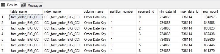
Each row is a single rowgroup within the columnstore index. Note that for each rowgroup, the min_data_id and max_data_id are the same. This indicates that the data is unordered, and the same set of disparate values is scattered across all rowgroups. The effect of this can be illustrated by running a simple analytic query.:

SET STATISTICS IO ON; --Output the IO that was needed to execute the query

SELECT SUM([Total Excluding Tax]) AS [Total Excluding Tax]
FROM dbo.fact_order_BIG_CCI
WHERE [Order Date Key] = '2014-12-04';

This query returns a sum for only a single date value. When executed, the output of statistics IO shows the following:

Table 'fact_order_BIG_CCI'. Scan count 1, logical reads 0, physical reads 0, page server reads 0, read-ahead reads 0, page server read-ahead reads 0, lob logical reads 1540, lob physical reads 0, lob page server reads 0, lob read-ahead reads 0, lob page server read-ahead reads 0.

Table 'fact_order_BIG_CCI'. Segment reads 8, segment skipped 0.

Note that 8 segments were read and 0 were skipped. This indicates that data had to be read from all rowgroups in order to return information for a single date. The reads (1547) are suspiciously high for such a simple query as well.

The next step for this demonstration is to order this data and rerun the above queries again.

To do this, the columnstore index will be swapped out for a clustered rowstore index that is ordered by Order Date Key. The clustered rowstore index will then be swapped for a clustered columnstore index. MAXDOP of 1 ensures that parallelism does not inadvertently result in unordered data via multiple streams of ordered data being shuffled together into new rowgroups: (The clustered index I create first orders the data in the object before we create the clustered columnstore index.)

CREATE CLUSTERED INDEX CCI_fact_order_BIG_CCI 
       ON dbo.fact_order_BIG_CCI ([Order Date Key]) WITH (DROP_EXISTING = ON);

CREATE CLUSTERED COLUMNSTORE INDEX CCI_fact_order_BIG_CCI 
       ON dbo.fact_order_BIG_CCI WITH (DROP_EXISTING = ON, MAXDOP = 1);

Rerunning the rowgroup metadata query from earlier returns the following:

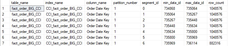
The minimum and maximum values for Order Date key are now nicely ordered from smallest to largest values. Running the simple analytic query from earlier produces the following statistics IO output:

Table 'fact_order_BIG_CCI'. Scan count 1, logical reads 0, physical reads 0, page server reads 0, read-ahead reads 0, page server read-ahead reads 0, lob logical reads 388, lob physical reads 0, lob page server reads 0, lob read-ahead reads 836, lob page server read-ahead reads 0.

Table 'fact_order_BIG_CCI'. Segment reads 1, segment skipped 6.

Only 1 segment was read whereas 6 were skipped. Note that the logical IO is significantly less than before, by about a factor of 10!

Filtering a large OLAP data set on ordered columnstore data will be significantly faster and more efficient than unordered data. But how is data ordered normally over the life span of a table? The most common solution is to:

1. Structure an analytic table to only accept insert and delete operations
2. Avoid updates at all costs.
3. Insert new data at the end of the table for the most recent date dimension.

Alternatively, if a large table needs to be converted to a columnstore index, then trickery as demonstrated above is necessary, ordering with a rowstore index and then swapping in a columnstore index on top of the newly ordered table.

Introducing: Ordered Columnstore Indexes!

SQL Server 2022 adds the ORDER clause to the clustered columnstore index creation syntax. This column list specifies which columns to sort columnstore data by as part of the rebuild operation or as part of an INSERT operation.

To alter our existing columnstore index to use this feature, the following syntax can be used:

CREATE CLUSTERED COLUMNSTORE INDEX CCI_fact_order_BIG_CCI ON dbo.fact_order_BIG_CCI
ORDER ([Order Date Key])
 WITH (DROP_EXISTING = ON, MAXDOP = 1);

The result of this change formalizes the order of the columnstore index to default to using Order Date Key. When the ORDER keyword is included in a columnstore index create statement, SQL Server will sort the data in TempDB based on the column(s) specified. In addition, when new data is inserted into the columnstore index, it will be pre-sorted as well. When an ordered clustered columnstore index is the target of an index rebuild operation, the column order specified earlier will be honored.

This feature sounds like the perfect solution to enable segment elimination, but it is in no way free. As implied by the use of the word SORT, SQL Server needs to expend resources to sort the data. This not only requires TempDB resources, but it is an OFFLINE operation. Therefore, swapping a clustered columnstore index for one that is sorted will result in rebuild operations going from being online to offline operations. Note that in a partitioned table, then operation will only be offline for partitions affected by the rebuild operation. Typically, this will be a single current-data partition. Therefore, partitioning can help in improving availability for much of the data in ordered clustered columnstore indexes.

The sort operation can be visualized by checking the execution plan for both a standard and ordered columnstore index.

If you look at the query plan for creating thee indexes, you will see some interesting differences. The following plan is for creating the non-ordered columnstore index built earlier in this article:

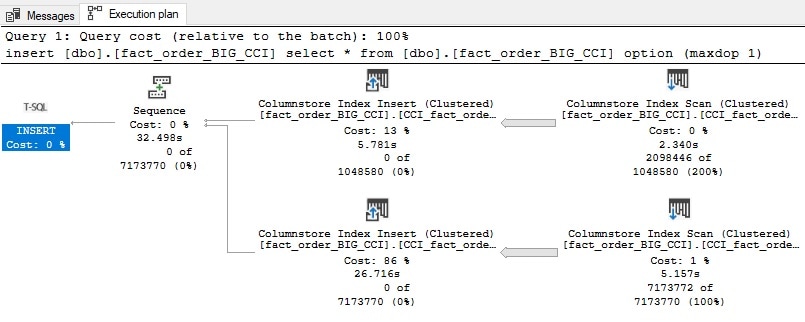
No surprises here. I wait 30 seconds and a columnstore index is ready for use on the table. Using the new syntax above that includes the ORDER clause will produce the following execution plan:

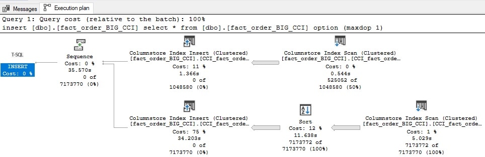
A SORT operation appears in the plan. Without partitioning or any other aids available, SQL Server needs to sort the entire data set in order to create an index that is ordered on the column of my choosing.

The column(s) used in the ORDER clause can be validated anytime in the system view sys.index_columns, using a query similar to this:

SELECT
     tables.name AS table_name,
     indexes.name AS index_name,
     columns.name AS column_name,
     index_columns.column_store_order_ordinal
FROM sys.index_columns
INNER JOIN sys.indexes
ON indexes.index_id = index_columns.index_id
AND indexes.object_id = index_columns.object_id
INNER JOIN sys.columns
ON index_columns.object_id = columns.object_id
AND columns.column_id = index_columns.column_id
INNER JOIN sys.tables
ON tables.object_id = indexes.object_id
WHERE tables.name = 'fact_order_BIG_CCI';

The results list all of the columns in the table, along with their column store order, if applicable. A value of zero indicates that the column is not a part of the columnstore order:

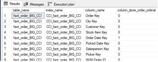
The metadata shows that Order Date Key is the sole ORDER column for this columnstore index. Consider a new index ordered by Order Date Key and then by Order Key:

CREATE CLUSTERED COLUMNSTORE INDEX CCI_fact_order_BIG_CCI ON dbo.fact_order_BIG_CCI
ORDER ([Order Date Key], [Order Key])
WITH (DROP_EXISTING = ON, MAXDOP = 1);

For this index, the metadata results from above show the additional column as part of the columnstore order:

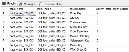
Note that Order Key is now shows as the second column in the columnstore order, after Order Date Key. For a large columnstore indexed table, ordering by an additional column may further assist queries that rely on multi-column filters.

Ordered Columnstore Index Notes and Considerations

It is worth repeating that only clustered columnstore indexes can be use the ORDER clause. Non-clustered columnstore indexes inherit data order from the underlying rowstore index structure during creation and will provide segment elimination as effectively as the underlying data allows.

Ordered columnstore indexes are a heavy-handed and somewhat imperfect way of improving data order and segment elimination for three reasons:

1. Rebuilding an ordered columnstore index is an OFFLINE operation.
2. Any data that is sorted must be sorted in TempDB.
3. If a sort operation is so large that it would spill to disk, then the sort is aborted and data order may not be perfect.

There is value in exploring each of these issues to ensure that decisions made regarding ordered columnstore indexes are as optimal as possible:

Rebuilds on an Ordered Columnstore Index = OFFLINE Operation (Per Partition)

This is an availability concern that will not impact all users of columnstore indexes. If dedicated maintenance windows exist for index maintenance and OFFLINE is acceptable for rebuild operations, then there is no issue to be had here. Index reorganization is still an ONLINE operation and can be used as part of regular maintenance to reduce the need for rebuilds.

The amount of time that a given partition is unavailable will be equal to the amount of time needed to sort and rebuild the data in that partition. Therefore, if rebuilding a partition with 20 million rows in a clustered columnstore index typically takes 30 seconds, then the same operation would result in at least 30 seconds of offline/downtime for the same index if it were ordered. Presumably the sort operation will require some additional time, increasing the overall time needed to some number greater than 30 seconds.

It is possible to use partition switching to increase availability, though whether that level of added complexity is desired or not is wholly up to you to decide.

Ordered Columnstore Indexes Sort in TempDB

Data needs to be sorted, and in SQL Server, TempDB is where this happens. As a result, to ensure that data is properly sorted, it is important that TempDB has enough space allocated for it. If 500MB of data is to be inserted into an ordered columnstore index, then there needs to be an additional 500MB of TempDB space available.

Similarly, if a 500GB columnstore index is being rebuilt into an ordered columnstore index, then 500GB+ of TempDB space will be required. Depending on the organization and its hardware,

If there is insufficient TempDB space available to store the incoming columnstore data, then don’t use this feature. Ensuring there is enough space, though, becomes more important due to the next challenge:

Sort Operations Do Not Complete in Their Entirety

What happens when an ordered columnstore index is rebuilt or inserted into and not enough space is available in TempDB? Not what is expected! Typically, if a sort operator in an execution plan requires more TempDB space than is allocated or available, it spills to disk to allocate enough space to complete the operation.

That is NOT what happens with ordered columnstore indexes. If the data to be sorted into an ordered columnstore index exceeds the space allocated by the memory grant, then the sort operation simply completes and is flagged internally as a soft sort. A soft sort will sort as many rows as it can, but when space runs out, it will stop. While this behavior ensures that write operations are fast and do not spill to disk, they also pose a hazard as it is not immediately clear that this behavior occurred without further research.

To illustrate a soft sort, the test table earlier will be dropped, recreated, and populated with ~27.8 million rows. TempDB will also be reduced to a relatively small size to ensure that there is not enough space available to fully sort this data. The following code handles the table drop, creation, and population:

DROP TABLE dbo.fact_order_BIG_CCI;

CREATE TABLE dbo.fact_order_BIG_CCI (
     [Order Key] [bigint] NOT NULL,
     [City Key] [int] NOT NULL,
     [Customer Key] [int] NOT NULL,
     [Stock Item Key] [int] NOT NULL,
     [Order Date Key] [date] NOT NULL,
     [Picked Date Key] [date] NULL,
     [Salesperson Key] [int] NOT NULL,
     [Picker Key] [int] NULL,
     [WWI Order ID] [int] NOT NULL,
     [WWI Backorder ID] [int] NULL,
     [Description] [nvarchar](100) NOT NULL,
     [Package] [nvarchar](50) NOT NULL,
     [Quantity] [int] NOT NULL,
     [Unit Price] [decimal](18, 2) NOT NULL,
     [Tax Rate] [decimal](18, 3) NOT NULL,
     [Total Excluding Tax] [decimal](18, 2) NOT NULL,
     [Tax Amount] [decimal](18, 2) NOT NULL,
     [Total Including Tax] [decimal](18, 2) NOT NULL,
     [Lineage Key] [int] NOT NULL);

-- Generate 27769440 rows in a heap:
INSERT INTO dbo.fact_order_BIG_CCI
SELECT
     [Order Key] + (250000 * ([Day Number] +
            ([Calendar Month Number] * 31))) AS [Order Key]
    ,[City Key]
    ,[Customer Key]
    ,[Stock Item Key]
    ,[Order Date Key]
    ,[Picked Date Key]
    ,[Salesperson Key]
    ,[Picker Key]
    ,[WWI Order ID]
    ,[WWI Backorder ID]
    ,[Description]
    ,[Package]
    ,[Quantity]
    ,[Unit Price]
    ,[Tax Rate]
    ,[Total Excluding Tax]
    ,[Tax Amount]
    ,[Total Including Tax]
    ,[Lineage Key]
FROM Fact.[Order]
CROSS JOIN
Dimension.Date
WHERE Date.Date <= '2013-04-30';

With a heap of data waiting to be sorted, trace flag 8666 will be enabled:

DBCC TRACEON (8666);

This undocumented trace flag will provide additional query optimizer details that otherwise are not provided in execution plans (graphical or XML). If you experiment with this trace flag, be sure to do so in a test environment and disable it when your testing is complete!

With added optimizer detail available, let’s turn on the actual execution plan, so we can quickly visualize what is going on here:

Finally, it is time to build an ordered columnstore index on the larger table created above:

CREATE CLUSTERED COLUMNSTORE INDEX CCI_fact_order_BIG_CCI ON dbo.fact_order_BIG_CCI
ORDER ([Order Date Key], [Order Key])
WITH (MAXDOP = 1)

This takes a few minutes to complete on my local server. The execution plan now contains some added information that can be used to understand what happened when SQL Server sorted the incoming data:

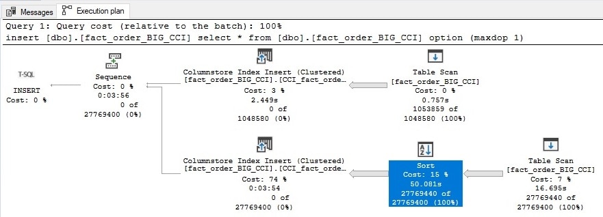
Opening the properties for the Sort operator allows us to get some additional detail:

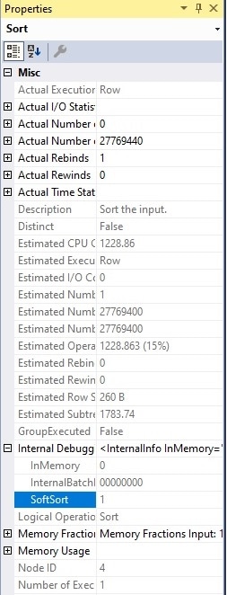
Within the internal debugger info is a flag that indicates if this was a soft sort or not. In this case, the answer is yes!

With that validated, the metadata query from earlier in this article will be run to show how well-ordered the rowgroups in the columnstore index are:

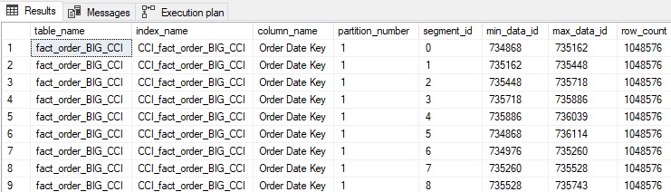
There are 27 rowgroups in total, but it is clear from the first 9 that this data is not actually ordered on Order Date Key effectively. While examining the values for min_data_id and max_data_id shows SOME ordering, it is clear that a query that should read 1-2 rowgroups will instead read many more as so many value ranges overlap.

To summarize: soft sorting is a hazard for building and maintaining ordered columnstore indexes and may be a reason to hold off on using them until the feature is further refined.

Conclusion

Prior to this feature, order was maintained manually. This sounds painful, but in reality, analytic data is often created based on date/time and naturally orders itself based on some key dimension(s), often date/time. For example, a table that loads new sales data daily will add a new day’s worth of data to the end of the columnstore index each day. So if updates are not performed on this table, then the data will naturally remain ordered as new data will also be the most recent. Even if 5% of the incoming data were old and out-of-order, overall segment elimination would still be relatively good.

Ordered columnstore indexes are an attempt to bring more focus on rowgroup elimination and its importance in speeding up analytic queries. If a columnstore index has 1 billion rows, then it will contain approximately 1,000 rowgroups. Reading 1000 segments to get data on a single column is far more expensive than reading 3 segments. Despite its promises, ordered columnstore indexes are not perfect and have limitations that make them a less-than-ideal solution, especially for tables where large amounts of data are inserted or rebuilt regularly.

This feature may work for you but be sure to test and ensure that insert operations and rebuilds do indeed sort the data correctly. If not, it may be worth reverting to the old-fashioned way of managing this data using natural ordering via manual processes.

Let’s hope for feature improvements! Columnstore indexes are a prime example of a feature that has improved steadily with every version of SQL Server since its inception. In the same way that columnstore indexes have matured to allow a wider variety of write operations, rowgroup elimination for more data types and predicates, and improved rowgroup consolidation/maintenance, it is likely that this feature will also get a much-needed upgrade soon.

 

The post Ordered Columnstore Indexes in SQL Server 2022 appeared first on Simple Talk.

from Simple Talk https://ift.tt/F0ogi2v
via

Modifying MySQL data from within Python

In the previous article in this series, I introduced you to how to access MySQL data from within a Python script. The article described how to use the MySQL Connector to establish a connection with a database and then retrieve data through that connection. In this article, I continue the discussion by demonstrating how to insert, update, and delete data in a MySQL database, again working with Python and the MySQL Connector.

The process of modifying MySQL data from within Python is, in many respects, similar to querying data. You must define a connection object that links to the database and define a cursor object based on that connection. You can then use the cursor object to execute your SQL statement. If you are not familiar with these concepts, I recommend that you read my previous article before launching into this one.

Although I focus specifically on Python and the MySQL Connector in this article (and in the last one), the process of connecting to a MySQL database and querying data is similar in most object-oriented programming environments, at least in the broader sense.

Each combination of programming language and database connector is unique, and you must understand how they work in your specific environment to use them effectively. That said, seeing how to interface with MySQL from within Python can still provide you with a conceptual understanding of what database access looks like in a programming language.

Note: The examples in this article are based on a specific MySQL and Python setup. The last section of the article—“Appendix: Preparing your Python and MySQL environment”—provides information about how I set up my system and includes a SQL script for creating the database and tables on which the examples are based.

Adding data to a MySQL database from within Python

The steps you take to insert data in a MySQL database are similar to those you follow to update or delete data. In each case, you generally take the following steps:

1. Import the mysql.connector module or specific its components.
2. Define a connection object that establishes a connection to the target database.
3. Use the connection object to invoke the cursor method and create a cursor object.
4. Define a SQL statement and save it to a variable.
5. Use the cursor object to invoke the execute method, passing in the variable as an argument.
6. Commit your changes to the database.
7. Close the cursor and the connection.

These steps are, of course, a simplification of the process, but they should provide you with an idea of what you’re trying to achieve. You can see these steps in the following Python script, which runs an INSERT statement against the manufacturers table in the travel database:

# import connect and Error modules
from mysql.connector import connect, Error

# define connection object
conn = connect(
  user='root',
  password='mysql_PW@327!xx',
  host='localhost',
  database='travel')

# open cursor
cursor = conn.cursor()

# try to run code block
try:
  # define INSERT statement
  add_manufacturer = ('INSERT INTO manufacturers '
    '(manufacturer_id, manufacturer) '
    'VALUES (101, \'Airbus\')')

  # run INSERT statement
  cursor.execute(add_manufacturer)

  # commit transaction
  conn.commit()

# catch exception, roll back transaction, print error message
except Error as err:
  conn.rollback()
  print('Error message: ' + err.msg)

# close cursor, close connection
finally:
  cursor.close()
  conn.close()

If you read the previous article, many of these elements should look familiar to you. The script starts by importing the connect and Error methods from the MySQL Connector module (mysql.connector). Next, the script instantiates a connection object and assigns it to the conn variable and then instantiates a cursor object and assigns it to the cursor variable. This is followed by a try block, where you define and run your SQL statement.

Note: I do want to remind you again that putting passwords, especially the root password, in a script that you store somewhere is not best security practice. A discussion of security is far beyond the scope of this article. It’s up to you to take the steps necessary to secure your application from the wide range of potential threats that can put your data at risk.

One thing you might notice that’s different in this script from the examples you saw in the previous article is that the connection and cursor objects are defined prior to the try block, rather than within it. This lets you access the objects outside of the try block, which I’ll explain shortly.

In the try block, I first defined the INSERT statement and assigned it to the add_manufacturer variable. I then used the cursor object to call the execute method, passing in the variable in as an argument. Because it contains the INSERT statement, the method will execute the statement when you run the script.

Next, I used the connection object to invoke the commit method. You must specially commit your changes to the database because by default, the MySQL Connector turns off MySQL’s autocommit feature, so your changes won’t be implemented until you commit them. (Note: you can control this with autocommit property on the connection object if you wish.)

I also used the connection object to invoke the rollback method, which I included in the except block. Because I defined the connection object outside of the try block, I can use the object in other blocks to invoke methods such as rollback. If a data-related error occurs, the transaction will be rolled back, undoing any changes that might have been made within the try block.

Something else I’ve included that wasn’t in the previous article is a finally block. A finally block is often used with a try block to run statements that should be executed whether or not an error occurs. In this way, you can ensure that the cursor and connection get closed even if there is a MySQL exception.

When you run the Python script the first time, it should insert the row in the manufacturers table with no problem. However, if you try to run the script a second time, MySQL will return a duplicate key error because the manufacturer_id value of 101 already exists. The manufacturer_id column is the table’s primary key, so a duplicate key error would be expected. In fact, this is an easy way to verify whether your script’s MySQL error handing is working as it should.

In the previous article, I also demonstrated how to use the %s marker as a placeholder within your SELECT statements. The marker makes it possible to create more dynamic SELECT statements based on user input. You can also use %s markers in your INSERT statements (as well as UPDATE and DELETE statements). The following Python script includes an INSERT statement that contains nine %s markers in the VALUES clause:

# import connect and Error modules
from mysql.connector import connect, Error

# define connection object
conn = connect(
  user='root',
  password='mysql_PW@327!xx',
  host='localhost',
  database='travel')

# open cursor
cursor = conn.cursor()

# try to run code block
try:
  # define INSERT statement
  add_airplane = ('INSERT INTO airplanes '
    '(plane_id, plane, manufacturer_id, engine_type, engine_count, '
      'wingspan, plane_length, max_weight, icao_code) '
    'VALUES (%s, %s, %s, %s, %s, %s, %s, %s, %s)')

  # define plane values for INSERT in a tuple
  plane_values = (1001, 'A340-600', 101, 'Jet', 4, 208.17, 247.24, 837756, 'A346')

  # run INSERT statement
  cursor.execute(add_airplane, plane_values)

  # commit transaction
  conn.commit()

# catch exception, roll back transaction, print error message
except Error as err:
  conn.rollback()
  print('Error message: ' + err.msg)

# close cursor, close connection
finally:
  cursor.close()
  conn.close()

After defining the INSERT statement, I created a tuple that contains the values that will be assigned to the markers, in the order they need to be inserted. I then assigned the tuple to the plane_values variable. (A tuple is an immutable collection of objects.) In the real world, you’ll likely want to capture the marker values through user interaction or other means, rather than hard-coding them in this way, but this approach should be enough to demonstrate how the markers work.

After defining my SQL statement and marker values, I used the cursor object to call the execute method and run the INSERT statement. I also included a second argument that specifies the plane_values variable. As a result, the %s markers in the INSERT statement will be replaced with the tuple values during statement execution. When you run the script the first time, the row should be added to the airplanes table with no problem.

In some cases, you’ll want to add multiple rows to a table in a single operation. You can do this in Python by making a few adjustments to the code, as shown in the following script:

# import connect and Error modules
from mysql.connector import connect, Error

# define connection object
conn = connect(
  user='root',
  password='mysql_PW@327!xx',
  host='localhost',
  database='travel')

# open cursor
cursor = conn.cursor()

# try to run code block
try:
  # define INSERT statement
  add_airplanes = ('INSERT INTO airplanes '
    '(plane_id, plane, manufacturer_id, engine_type, engine_count, '
      'wingspan, plane_length, max_weight, icao_code) '
    'VALUES (%s, %s, %s, %s, %s, %s, %s, %s, %s)')

  # define plane values for INSERT in an list of tuples
  plane_values = [
    (1002, 'A350-800 XWB', 101, 'Jet', 2, 212.42, 198.58, 546700, 'A358'),
    (1003, 'A350-900', 101, 'Jet', 2, 212.42, 219.16, 617295, 'A359'),
    (1004, 'A380-800', 101, 'Jet', 4, 261.65, 238.62, 1267658, 'A388'),
    (1005, 'A380-843F', 101, 'Jet', 4, 261.65, 238.62, 1300000, 'A38F')]

  # run INSERT statement
  cursor.executemany(add_airplanes, plane_values)

  # commit transaction
  conn.commit()

# catch exception, roll back transaction, print error message
except Error as err:
  conn.rollback()
  print('Error message: ' + err.msg)

# close cursor, close connection
finally:
  cursor.close()
  conn.close()

The INSERT statement in this script is the same one as in the previous example. However, the tuple assigned to the plane_values variable has been replaced by a list that includes four tuples containing the %s values for the INSERT statement. Each tuple corresponds to one row of data that will be inserted into the airplanes table.

Another difference in this example from the previous one is that the cursor object is now used to invoke the executemany method rather than the execute method. The executemany method makes it easy to use a single INSERT statement to add multiple rows to a table, while still taking advantage of the %s markers. When you run this Python script, it should now add the four rows to the airplanes table.

You can, of course, define an INSERT statement that includes all the rows, without using the %s markers, but then you lose the advantage of the markers and their potential for creating dynamic queries. Even so, it’s good to know that you can create a single statement if you want to go this route.

You can also define multiple SQL statements within your Python code. For example, the following Python script adds a row to the manufacturers table and then adds five rows to the airplanes table for that manufacturer:

# import connect and Error modules
from mysql.connector import connect, Error

# define connection object
conn = connect(
  user='root',
  password='mysql_PW@327!xx',
  host='localhost',
  database='travel')

# open cursor
cursor = conn.cursor()

# try to run code block
try:
  # define manufacturers INSERT statement
  add_manufacturer = ('INSERT INTO manufacturers '
    '(manufacturer_id, manufacturer) '
    'VALUES (%s, %s)')

  # define manufacturer values for INSERT
  manufacturer_values = (102, 'Beagle Aircraft Limited')

  # run manufacturers INSERT statement
  cursor.execute(add_manufacturer, manufacturer_values)

  # define airplanes INSERT statement
  add_airplanes = ('INSERT INTO airplanes '
    '(plane_id, plane, manufacturer_id, engine_type, engine_count, '
      'wingspan, plane_length, max_weight, icao_code) '
    'VALUES (%s, %s, %s, %s, %s, %s, %s, %s, %s)')

  # define plane values for INSERT
  plane_values = [
    (1006, 'A.109 Airedale', 102, 'Piston', 1, 36.33, 26.33, 2750, 'AIRD'),
    (1007, 'A.61 Terrier', 102, 'Piston', 1, 36, 23.25, 2400, 'AUS6'),
    (1008, 'B.121 Pup', 102, 'Piston', 1, 31, 23.17, 1600, 'PUP'),
    (1009, 'B.206', 102, 'Piston', 2, 55, 33.67, 7500, 'BASS'),
    (1010, 'D.5-108 Husky', 102, 'Piston', 1, 36, 23.17, 2400, 'D5')]

  # run airplanes INSERT statement
  cursor.executemany(add_airplanes, plane_values)

  # commit transaction
  conn.commit()

# catch exception, roll back transaction, print error message
except Error as err:
  conn.rollback()
  print('Error message: ' + err.msg)

# close cursor, close connection
finally:
  cursor.close()
  conn.close()

The script first defines the INSERT statement for the manufacturers table, adds a tuple for the statement’s %s values, and then invokes the execute method to run the statement. Next, the script defines the INSERT statement for the airplanes table, adds a list of tuples for the %s values, and then invokes the executemany method to run the second statement. After running the two statements, the script commits the transaction.

Updating data in a MySQL database from within Python

The process of updating MySQL data from within Python works much the same as inserting data, except that you define an UPDATE statement instead of an INSERT statement. For example, the following Python script modifies a row in the airplanes table:

# import connect and Error modules
from mysql.connector import connect, Error

# define connection object
conn = connect(
  user='root',
  password='mysql_PW@327!xx',
  host='localhost',
  database='travel')

# open cursor
cursor = conn.cursor()

# try to run code block
try:
  # define UPDATE statement
  update_plane = ("UPDATE airplanes "
    "SET plane = 'D.5/108 Husky' WHERE plane_id = %s")

  # define plane_id value for UPDATE as a tuple
  id_value = (1010,)

  # run UPDATE statement
  cursor.execute(update_plane, id_value)

  # commit transaction
  conn.commit()

# catch exception, roll back transaction, print error message
except Error as err:
  conn.rollback()
  print('Error message: ' + err.msg)

# close cursor, close connection
finally:
  cursor.close()
  conn.close()

You should recognize most of the elements in this script. The UPDATE statement changes the plane value for the row that has a plane_id value of 1010. This in itself should be fairly straightforward, but take particular note of the id_value variable and its assignment.

The UPDATE statement includes only one %s marker, so you need to define only one value outside the statement. In this case, however, the assigned value, 1010, is followed by a comma and enclosed in parentheses. This is because the execute method will accept only a list, tuple, or dictionary for the second argument, not a simple string or integer. To accommodate this requirement, I created a tuple by adding the trailing comma and then enclosing the value and comma in parentheses. Now I can then use the id_value variable as the second argument of the execute method.

When modifying MySQL data, you can create more complex SQL statements than what I showed you in the previous script. For example, the following UPDATE statement includes a subquery in its WHERE clause:

# import connect and Error modules
from mysql.connector import connect, Error

# define connection object
conn = connect(
  user='root',
  password='mysql_PW@327!xx',
  host='localhost',
  database='travel')

# open cursor
cursor = conn.cursor()

# try to run code block
try:
  # define UPDATE statement
  update_planes = ("UPDATE airplanes "
    "SET wingspan = ROUND(wingspan), plane_length = ROUND(plane_length) "
    "WHERE manufacturer_id = "
      "(SELECT manufacturer_id FROM manufacturers "
      "WHERE manufacturer = %s)")

  # define plane_id value for UPDATE
  manufacturer = ('Beagle Aircraft Limited',)

  # run UPDATE statement
  cursor.execute(update_planes, manufacturer)

  # commit transaction
  conn.commit()

# catch exception, roll back transaction, print error message
except Error as err:
  conn.rollback()
  print('Error message: ' + err.msg)

# close cursor, close connection
finally:
  cursor.close()
  conn.close()

The subquery retrieves the manufacturer_id value for the manufacturer specified in the manufacturer variable. The manufacturer_id value is then used to determine which rows in the airplanes table to update. (I covered subqueries in an earlier article in this series, so refer to that if you have any questions about how they work.)

In the previous two examples, the UPDATE statements included only one %s marker, but you can include multiple markers in your statements, as in the following Python script:

# import connect and Error modules
from mysql.connector import connect, Error

# define connection object
conn = connect(
  user='root',
  password='mysql_PW@327!xx',
  host='localhost',
  database='travel')

# open cursor
cursor = conn.cursor()

# try to run code block
try:
  # define UPDATE statement
  update_plane = ("UPDATE airplanes "
    "SET wingspan = wingspan + %s, plane_length = plane_length + %s "
    "WHERE plane_id = %s")

  # define values for UPDATE in a tuple
  plane_values = (5, 8, 1005)

  # run UPDATE statement
  cursor.execute(update_plane, plane_values)

  # commit transaction
  conn.commit()

  # define SELECT statement
  select_query = (
    "SELECT plane_id, plane, wingspan, plane_length "
    "FROM airplanes WHERE plane_id = %s")

  # run SELECT statement
  cursor.execute(select_query, (plane_values[2],))
  results = cursor.fetchone()

  # print query results
  print('Rows updated:', cursor.rowcount)
  print('plane_id:', results[0])
  print('plane:', results[1])
  print('new wingspan:', results[2])
  print('new plane_length:', results[3])

# catch exception, roll back transaction, print error message
except Error as err:
  conn.rollback()
  print('Error message: ' + err.msg)

# close cursor, close connection
finally:
  cursor.close()
  conn.close()

The UPDATE statement contains two %s markers in the SET clause and one in the WHERE clause. The values for these markers are in a tuple that I assigned to the plane_values variable. You can use as many %s markers as needed in whatever clauses you deem necessary. Just remember to specify their values in the correct order so they match the statement.

After I ran the UPDATE statement and called the commit method, I defined a SELECT statement to retrieve the newly updated data from the airplanes table. I did this as a way to verify that the data had been correctly modified.

When I called the execute method to run the SELECT statement, I passed in the value from the plane_values tuple, specifying 2 as the value’s index number. (Tuples use a 0-based index.) I also added a comma after the index number and enclosed the entire value in parentheses so it would be treated as its own tuple, as required by the execute method.

I then used the cursor object to run the fetchone method, which retrieves the current row from the query results. Next, I saved the row of values—returned as a single tuple—to the results variable.

I followed this with a series of print statements that display information about the update. The first print statement calls the rowcount property on the cursor object. The property shows the number of rows that were affected by the UPDATE statement. This is followed by four more print statements, one for each value in the row returned by the SELECT statement. Each print statement uses the tuple’s index to specify which value to include. The returned information should look similar to the following:

Rows updated: 1
plane_id: 1005
plane: A380-843F
new wingspan: 266.65
new plane_length: 246.62

The original wingspan value was 261.65, and the original plane_length value was 238.62. When you add 5 and 8 to these values, respectively, you get the new totals returned by the script. You can also add logic to your script to capture the old values before updating them. In that way, you can return both the old and new values at the end of your script and pass those onto your application.

Deleting data in a MySQL database from within Python

The process of deleting MySQL data from within Python is much the same as inserting or updating it. For example, the following Python script deletes a row from the airplanes table:

# import connect and Error modules
from mysql.connector import connect, Error

# define connection object
conn = connect(
  user='root',
  password='mysql_PW@327!xx',
  host='localhost',
  database='travel')

# open cursor
cursor = conn.cursor()

# try to run code block
try:
  # define DELETE statement
  delete_plane = ("DELETE FROM airplanes "
    "WHERE plane_id = %s")

  # define plane_id value for DELETE in a tuple
  plane_id = (1010,)

  # run DELETE statement
  cursor.execute(delete_plane, plane_id)
  print('Number of rows deleted: ', cursor.rowcount)

  # commit transaction
  conn.commit()

# catch exception, roll back transaction, print error message
except Error as err:
  conn.rollback()
  print('Error message: ' + err.msg)

# close cursor, close connection
finally:
  cursor.close()
  conn.close()

At this point, you should be familiar with all the elements in this script. I defined a DELETE statement and assigned it to the delete_plane variable. I then assigned a value to the plane_id variable, which will be used for the %s marker. Next, I executed the statement, specifying the two variables, and added a print statement to display the number of rows that were deleted.

Overall, there’s nothing really new about this script except for the use of a DELETE statement rather than INSERT or UPDATE. I simply wanted to show you what deleting data might look like. You can make your DELETE statements as complex as necessary and use more %s markers where needed, as in the next example:

# import connect and Error modules
from mysql.connector import connect, Error

# define connection object
conn = connect(
  user='root',
  password='mysql_PW@327!xx',
  host='localhost',
  database='travel')

# open cursor
cursor = conn.cursor()

# try to run code block
try:
  # define DELETE statement
  delete_plane = ("DELETE FROM airplanes "
    "WHERE manufacturer_id = %(mfc_id)s AND max_weight < %(weight)s")

  # define values for DELETE in a tuple
  plane_values = {'mfc_id': 102, 'weight': 5000}

  # run DELETE statement
  cursor.execute(delete_plane, plane_values)
  print('Number of rows deleted: ', cursor.rowcount)

  # commit transaction
  conn.commit()

# catch exception, roll back transaction, print error message
except Error as err:
  conn.rollback()
  print('Error message: ' + err.msg)

# close cursor, close connection
finally:
  cursor.close()
  conn.close()

In this script, I’ve used a different form of the %s markers. When I defined the marker values, I created a dictionary rather than a tuple or list. A dictionary makes it possible to assign a label to each value. You can then reference that label within your SQL statement. To do so, insert the label name, enclosed in parentheses, between the % and the s, as in %(mfc_id)s. You can reference any value in the dictionary, without regard to their order.

Getting started with Python and MySQL data modifications

In this article and the previous one, I’ve tried to provide you with a foundation for using the MySQL Connector in your Python scripts. There is, of course, much more to the connector and MySQL that what I’ve shown you here. There’s also a lot more to writing data-driven scripts and applications. But the information I’ve provided should at least help you better understand how to connect to a MySQL database from within Python and manipulate the data. You might also find this information useful when working with other programming languages, at least from a conceptual vantage point. Data is at the heart of most applications, and the more insight you have into how the pieces fit together, the greater you’ll be able to appreciate what it takes to make these applications work.

Appendix: Preparing your MySQL and Python environment

For the examples in this article, I used a Mac computer that was set up with the following components:

• MySQL 8.0
• Python 3.10
• PyCharm Community Edition IDE
• MySQL Connector/Python 8.0 module

You can find information about installing the module in the MySQL documentation. On my system, I used pip to add the module. Pip is a package installer for Python that makes it very easy to deploy a module.

The Python examples in this article connect to the travel database on a local MySQL instance. The database contains the manufacturers table and airplanes table, which is defined with a foreign key that references the manufacturers table. This is the same database and tables you saw in previous articles in this series, except that you don’t need to insert any data.

If you plan to try out these examples, start by running the following script against your MySQL instance:

DROP DATABASE IF EXISTS travel;

CREATE DATABASE travel;

USE travel;

CREATE TABLE manufacturers (
  manufacturer_id INT UNSIGNED NOT NULL,
  manufacturer VARCHAR(50) NOT NULL,
  create_date TIMESTAMP NOT NULL DEFAULT CURRENT_TIMESTAMP,
  last_update TIMESTAMP NOT NULL 
    DEFAULT CURRENT_TIMESTAMP ON UPDATE CURRENT_TIMESTAMP,
  PRIMARY KEY (manufacturer_id) );

CREATE TABLE airplanes (
  plane_id INT UNSIGNED NOT NULL,
  plane VARCHAR(50) NOT NULL,
  manufacturer_id INT UNSIGNED NOT NULL,
  engine_type VARCHAR(50) NOT NULL,
  engine_count TINYINT NOT NULL,
  max_weight MEDIUMINT UNSIGNED NOT NULL,
  wingspan DECIMAL(5,2) NOT NULL,
  plane_length DECIMAL(5,2) NOT NULL,
  parking_area INT GENERATED ALWAYS AS ((wingspan * plane_length)) STORED,
  icao_code CHAR(4) NOT NULL,
  create_date TIMESTAMP NOT NULL DEFAULT CURRENT_TIMESTAMP,
  last_update TIMESTAMP NOT NULL 
    DEFAULT CURRENT_TIMESTAMP ON UPDATE CURRENT_TIMESTAMP,
  PRIMARY KEY (plane_id),
  CONSTRAINT fk_manufacturer_id FOREIGN KEY (manufacturer_id) 
    REFERENCES manufacturers (manufacturer_id) );

The script will create the travel database and add the manufacturers and airplanes tables in the proper order to accommodate the foreign key defined in the airplanes table. If you already created the database and tables for previous articles, I recommend that you re-create them now to ensure that your key values line up correctly with the examples.

 

The post Modifying MySQL data from within Python appeared first on Simple Talk.

from Simple Talk https://ift.tt/O8RqGrA
via

GENERATE_SERIES: My new go-to to build sets

I have come across a lot of use cases for manufacturing rows on the fly, aside from the common goal of populating a large data set such as a numbers or calendar table. A few favorites include building sample data, pivoting an unknown number of columns, data extrapolation, and filling gaps in date or time ranges.

If you are on SQL Server 2022 or Azure SQL Database, or have been reading up on new features, you’ve likely heard about one of the better T-SQL enhancements: a new built-in function called GENERATE_SERIES. The syntax is straightforward – it accepts arguments for start and stop, and an optional argument to indicate step (in case you want to iterate by more than 1, or backwards):

SELECT value FROM GENERATE_SERIES(<start>, <stop> [, <step>]);

A few quick examples:

/* count to 6 */ 
 SELECT [1-6] = value 
   FROM GENERATE_SERIES(1, 6);

 /* count by 5s to 30 */
 SELECT [step 5] = value 
   FROM GENERATE_SERIES(5, 30, 5);

 /* count from 10 to 0, backwards, by 2 */
 SELECT [backward] = value
   FROM GENERATE_SERIES(10, 0, -2);

 /* get all the days in a range, inclusive */
 DECLARE @start date = '20230401',
         @end   date = '20230406';

 SELECT [days in range]  = DATEADD(DAY, value, @start)
   FROM GENERATE_SERIES(0, DATEDIFF(DAY, @start, @end));

Results:

1-6 (first resultset)		step 5 (second resultset)		backward (third resultset)		days in range (fourth resultset)
1		5		10		2023-04-01
2		10		8		2023-04-02
3		15		6		2023-04-03
4		20		4		2023-04-04
5		25		2		2023-04-05
6		30		0		2023-04-06

 

That is some handy syntax that is quite easy to use. I dug in more about it during the beta, but…

How would we do this on older versions of SQL Server?

We’ve been generating sets since before SQL Server was SQL Server, so we’ve always found a way. Some approaches are cryptic, and some perform poorly; others are cryptic and perform poorly. I have two that I like: one that works in SQL Server 2016 and above, and one that works all the way back to SQL Server 2008. There are others (even some that will work on SQL Server 2000), but these are the two I want to focus on today.

I’m going to present both techniques as inline table-valued functions, since the logic is complicated enough to justify encapsulation, and that also happens to keep demos nice and tidy. These will be written to accommodate a series of up to 4,000 values – we can certainly go beyond that, but exceeding 8,001 values leads to the first solution requiring LOB support, which can do unpredictable things to performance. The second is capped at 4,096 values because it is the highest power of 4 that is also less than 8,001; you’ll see why that’s important in a moment.

2016+ STRING_SPLIT + REPLICATE

This one is a rather recent addition to my toolbox; I don’t recall where I first came across it, but I like it because it’s concise without being overly opaque. We determine the number of values we want in our sequence, less one – which is the stop minus the start. We use REPLICATE to generate a string that is a sequence of that many commas. Then we split that string using STRING_SPLIT, which results in { stop - start + 1 } empty strings. We then apply a ROW_NUMBER() to the output, which serves as our series. Since our starting value might not be 1, we add it to the row number, and subtract 1.

To get started, I will create a new database named GenSeries to put the sample code.

CREATE FUNCTION dbo.GenerateSeries_Split
 (
   @start int,
   @stop  int
 )
 RETURNS TABLE WITH SCHEMABINDING
 AS
   RETURN
   (
     SELECT TOP (@stop - @start + 1) 
       value = ROW_NUMBER() OVER (ORDER BY @@SPID) + @start - 1
     FROM STRING_SPLIT(REPLICATE(',', @stop - @start), ',')
     ORDER BY value
   );

To support a range greater than 8,001 values, you can change this line:

FROM STRING_SPLIT(REPLICATE(CONVERT(varchar(max),','), @stop - @start), ',')

…but that’s not the version I’m going to test today.

2008+ Cross-Joined CTEs

This solution reaches further back into most of the unsupported versions of SQL Server you might still be clinging to but, unfortunately, it is a little more cryptic. I remember first using it in this solution after discovering this really efficient implementation by Jonathan Roberts.

CREATE FUNCTION dbo.GenerateSeries_CTEs
 (
   @start int,
   @stop  int
 )
 RETURNS TABLE WITH SCHEMABINDING 
 AS 
   RETURN
   (
     /* could work in 2005 by changing VALUES to a UNION ALL */
     WITH n(n) AS (SELECT 0 FROM (VALUES (0),(0),(0),(0)) n(n)),
      i4096(n) AS (SELECT 0 FROM n a, n b, n c, n d, n e, n f)      
     SELECT TOP (@stop - @start + 1) 
       value = ROW_NUMBER() OVER (ORDER BY @@TRANCOUNT) + @start - 1 
     FROM i4096
     ORDER BY value
   );

This approach uses two CTEs – one that just generates 4 rows using a VALUES constructor; the second one cross joins it to itself, however many times is necessary to cover the range of values you need to support. (In our case, we want to support 4,000 values.)

Each time you cross join the original set of 4, you produce a Cartesian product of 4^n, where n is bumped by 1 for each new reference. So if you just named it once, you’d have 4^1, which is 4. The second reference is 4^2, which is 16. Then 4^3 = 64, 4^4 = 256, 4^5 = 1,024, and 4^6 = 4,096. I’ll try to illustrate in an image:

If you only need to support 256 values, for example, then you could change that second line to stop at the 4th cross join:

i256(n) AS (SELECT 0 FROM n a, n b, n c, n d)

And if you needed more than 4,096 values – say, up to 16,384 – you would instead just add one additional cross join:

i16K(n) AS (SELECT 0 FROM n a, n b, n c, n d, n e, n f, n g)

And of course you can be more verbose and self-documenting. Technically, I would want to write the following, it’s just a lot more to digest on first glance:

i4096(n) AS 
        (
           SELECT 0 FROM n AS n4    CROSS JOIN n AS n16 
              CROSS JOIN n AS n64   CROSS JOIN n AS n256
              CROSS JOIN n AS n1024 CROSS JOIN n AS n4096
           /* ... */
        )

You could also code defensively and alter the parameters to smallint or tinyint to prevent surprises when someone uses an int value that is too large and they don’t get the full set they expect. This won’t raise an error, unless you also add additional handling, say, to divide by 0 somewhere if the range is too large. Keep in mind that someone could try to generate 100 rows by passing in a start parameter of 2,000,000,000 and a stop parameter of 2,000,000,100 – so restricting either input value instead of the difference might be unnecessarily limiting.

I often see recursive CTEs suggested for set generation, since they are a little less cryptic than this, and are somewhat self-documenting (if you already understand recursive CTEs, I suppose). I do like recursive CTEs generally, and have offered them up in many posts and answers, but they’re not ideal for broad consumption in this context unless you will never retrieve more than 100 rows (say, generating the days for a monthly report). This is because you will need a MAXRECURSION query hint to produce more than 100 values; since you can’t put that hint inside a function, it means you have to put it on every outer query that references the function. Ick! So much for encapsulation.

So how do they perform?

I thought about the simplest test I can do to pit different number generation techniques against each other, and the first that came to mind involves pagination. (Note: This is a contrived use case and not intended to be a discussion about the best ways to paginate data.)

In the GenSeries database, I will create a simple table with 4,000 rows:

SELECT TOP (4000) rn = IDENTITY(int,1,1),*
 INTO dbo.things FROM sys.all_columns;

 CREATE UNIQUE CLUSTERED INDEX cix_things ON dbo.things(rn);

Then I created three stored procedures. One that uses the split approach:

CREATE OR ALTER PROCEDURE dbo.PaginateCols_Split
   @PageSize int = 100,
   @PageNum  int = 1
 AS
 BEGIN
   SET NOCOUNT ON;

   DECLARE @s int = (@PageNum-1) * @PageSize + 1;
   DECLARE @e int = @s + @PageSize - 1;

   WITH r(rn) AS
   (
     SELECT TOP (@PageSize) rn = value
     FROM dbo.GenerateSeries_Split(@s, @e)
   )
   SELECT t.* FROM dbo.things AS t 
   INNER JOIN r ON t.rn = r.rn;
 END

One that uses stacked CTEs:

CREATE OR ALTER PROCEDURE dbo.PaginateCols_CTEs
   @PageSize int = 100,
   @PageNum  int = 1
 AS
 BEGIN
   SET NOCOUNT ON;

   DECLARE @s int = (@PageNum-1) * @PageSize + 1;
   DECLARE @e int = @s + @PageSize - 1;

   WITH r(rn) AS
   (
     SELECT TOP (@PageSize) rn = value
     FROM dbo.GenerateSeries_CTEs(@s, @e)
   )
   SELECT t.* FROM dbo.things AS t 
   INNER JOIN r ON t.rn = r.rn;
 END

And one that uses GENERATE_SERIES directly:

CREATE OR ALTER PROCEDURE dbo.PaginateCols_GenSeries
   @PageSize int = 100,
   @PageNum  int = 1
 AS
 BEGIN
   SET NOCOUNT ON;

   DECLARE @s int = (@PageNum-1) * @PageSize + 1;
   DECLARE @e int = @s + @PageSize - 1;

   WITH r(rn) AS
   (
     SELECT TOP (@PageSize) rn = value
     FROM GENERATE_SERIES(@s, @e)
   )
   SELECT t.* FROM dbo.things AS t 
   INNER JOIN r ON t.rn = r.rn;
 END

Then I created a wrapper that will call each of them with a defined page number – this way I could test the beginning, middle, and end of the set (pagination often sees tanking performance as the page number gets higher). This table is hardly a performance nightmare but if I ran the procedures enough times I would hopefully see some variance.

CREATE OR ALTER PROCEDURE dbo.PaginateCols_Wrapper
   @PageNum int = 1
 AS
 BEGIN
   SET NOCOUNT ON;

   EXEC dbo.PaginateCols_Split     @PageNum = @PageNum;
   EXEC dbo.PaginateCols_CTEs      @PageNum = @PageNum;
   EXEC dbo.PaginateCols_GenSeries @PageNum = @PageNum;
 END

If you execute this procedure, you will see 3 output sets that contain rows from sys.columns. If you vary the @pagenum parameter value, you will see different pages of data from that set, but each three will be the same results. The only difference is the series generating code.

I turned on Query Store, and always want to remind you that QUERY_CAPTURE_MODE = ALL is not a production-friendly option – but quite handy if you want to make sure you capture every instance of every query:

ALTER DATABASE GenSeries SET QUERY_STORE 
 (
   OPERATION_MODE              = READ_WRITE,
   QUERY_CAPTURE_MODE          = ALL /* Do not do this in production! */
 );

I didn’t want to run the procedures a bunch of times manually; I like using sqlstresscmd because I can run tests hundreds of thousands of times without guilt about overwhelming a poor UI, or waiting for results to render, or battling resource conflicts and poisoning the test as a result. It runs the queries, discards the results, and that’s it.

I configured a JSON file called GenSeries.json like this, to run each procedure 10,000 times across 16 threads. It took about 5 minutes to run on average:

{
   "CollectIoStats": true,
   "CollectTimeStats": true,
   "MainDbConnectionInfo": 
   {
     "Database": "GenSeries",
     "Login": "sa",
     "Password": "$tr0ng_P@$$w0rd",
     "Server": "127.0.0.1,2022"
   },
   "MainQuery": "EXEC dbo.PaginateCols_Wrapper @PageNum = 1;",
   "NumIterations": 10000,
   "NumThreads": 16,
   "ShareDbSettings": true
 }

Then ran it using the following:

sqlstresscmd -s ~/Documents/GenSeries.json

Then I collected the average runtimes from Query Store:

SELECT qt.query_sql_text,
        avg_duration       = AVG(rs.avg_duration/1000.0)
   FROM sys.query_store_query_text AS qt
   INNER JOIN sys.query_store_query AS q 
     ON qt.query_text_id = q.query_text_id
   INNER JOIN sys.query_store_plan  AS p 
     ON q.query_id = p.query_id
   INNER JOIN sys.query_store_runtime_stats AS rs 
     ON p.plan_id = rs.plan_id
   WHERE qt.query_sql_text LIKE N'%dbo.things%'
     AND qt.query_sql_text NOT LIKE N'%sys.query_store%'
   GROUP BY qt.query_sql_text;

When I wanted to switch to the middle or the end of the set, I ran this query to clear Query Store data. (Note: you will need to capture the results from Query Store each time before executing this statement as this clears everything from Query Store):

ALTER DATABASE GenSeries SET QUERY_STORE CLEAR;

Then I changed the MainQuery line appropriately to run tests for the middle and the end. For rows 1,901 – 2,000:

"MainQuery": "EXEC dbo.PaginateCols_Wrapper @PageNum = 20;",

And for rows 3,901 – 4,000:

"MainQuery": "EXEC dbo.PaginateCols_Wrapper @PageNum = 40;",

Here are the timing results in milliseconds (click to enlarge):

In these tests, the split approach was the winner, but the new built-in function is right on its heels. The stacked CTEs, while much more backward-compatible, have become a bit of an outlier.

I would love to see some flat lines in there, of course, since there shouldn’t be any penalty for jumping ahead to any page; but, not the point today. I do plan to revisit some of my old pagination techniques in a future article.

Conclusion

As the title suggests, I’m pretty happy with the syntax of GENERATE_SERIES so far, and I hope you get to try it out sooner than later! The performance of the split approach is slightly better, but both are still relatively linear and, for the simplicity of the implementation, I’d be inclined to use the newer syntax in most cases. At this scale, we’re talking about single-digit milliseconds anyway, so maybe not all that telling other than “this is worth testing.”

And to reiterate, this wasn’t meant to show that any of these methods might be better for pagination specifically – it was a completely manufactured scenario where the table just happened to have contiguous row numbers to join to the output. This was more a demonstration of how easy it is to swap GENERATE_SERIES into places where you’re using more convoluted methods today.

Further reading

As far as series generation goes, there are other options out there, too, including some from Paul White, Itzik Ben-Gan, and others in this 6-part Number series generator challenge from 2021. In particular, there is an interesting solution from Paul White (dbo.GetNums_SQLkiwi) in solutions part 4, but it does require a little concentration, and is version-limiting (it requires a table with a clustered columnstore index). You should do more thorough testing with his and other approaches from that series, with your data and workload, especially if your primary objective is squeezing performance. Some solutions will only be options if you are on modern versions and/or have some leeway in implementation (some CLR solutions might be interesting as well).

The post GENERATE_SERIES: My new go-to to build sets appeared first on Simple Talk.

from Simple Talk https://ift.tt/D8qQF7I
via

A Beginners Guide to MySQL Replication Part 1

MySQL Replication is a process where data from one MySQL database known as the source (formerly called “master”) is copied over to one or more other databases called replicas (formerly called “slaves”). Think of this like having a backup buddy that is always in sync and up to date, giving you peace of mind.

It’s important to highlight that in 2020, MySQL took the step to modernize its language by retiring outdated terms such as ‘master’ and ‘slave’ and replacing them with more inclusive language – ‘source’ and ‘replica’. The company is actively working towards updating its queries and documentation with these updated terms. According to the official blog post, the origin of these words is negative and does not fit the description.

Note that some of the syntax will still reference the old terms.

There are several benefits to using MySQL replication. For starters, it helps to increase the reliability and availability of your data. If the source database goes down, one of the replica databases can step in to take its place, keeping your application running smoothly. Plus, by distributing the load across multiple servers, replication can help to improve performance and prevent downtime. Another bonus? Replication makes it easier to back up and recover your data. So, if anything were to happen, you can rest easy knowing that you have a backup ready to go.

We have different types of replication setups, such as asynchronous, semi-synchronous, and synchronous replication. These are the standard replication types mentioned in the documentation. In this series, we’ll be delving into each of these replication types and examining their requirements, benefits, and limitations. So, hold on tight, as we embark on a journey of discovery to setting up and choosing the right replication method.

Types of MySQL Replication

The choice of replication method depends on the specific requirements of your application. There are various replication types available in MySQL, each having its pros and limitations:

Asynchronous replication:

This is a type of replication in MySQL that involves a single source server that receives all write operations and one or more replica servers that replicate the data from the source. This type of replication is useful for scaling read-only operations. The source server does not wait for acknowledgment from the replica servers before committing changes. Here are some of the benefits of asynchronous replication:

• Scalability: Asynchronous replication allows you to scale out the number of replica servers to meet growing demands for read-only access to data.
• Performance: Asynchronous replication allows the source server to commit changes to the database immediately, which can provide high performance as the source server does not need to wait for the replica servers to catch up.
• Flexibility: Asynchronous replication allows you to locate replica servers in different geographic locations, providing access to data from multiple regions.

Potential Limitations: Asynchronous replication is a great solution for businesses looking to scale their read-only operations and ensure high scalability. However, it may not be the best fit for applications that require real-time updates and immediate consistency due to some of its downsides, such as:

• Data consistency: Since the source server does not wait for the replica servers to catch up before committing changes, there may be a temporary loss of data in the event of a failure. This can result in a lack of consistency between the source and replica servers.
• Recovery time: If a failure occurs on the source server, it may take longer to recover and restore data consistency as the replica servers may have lagged.
• Lagging: Since the replica servers may not be in real-time sync with the source, there may be a lag in the replication process that can result in outdated data on the replica servers.

Synchronous Replication

This is a method of replicating data where the source server waits for acknowledgment from the replica servers before committing changes to the database. This ensures that data remains consistent across all servers and eliminates the risk of temporary data loss in the event of a failure. There are several benefits to using synchronous replication, some of which are:

• Data consistency and reliability: One of the key benefits of synchronous replication is the high level of data consistency and reliability it provides. With this method, you can be confident that all servers in your environment have the same up-to-date information, even in the event of a failure.
• Fast recovery time: It can provide a faster recovery time in the event of a failure, as the replica servers already have the latest data. This can be especially important in high-availability environments where you need to ensure minimal downtime.

Potential Limitations: However, just like for asynchronous, there are also some limitations to synchronous replication that you should be aware of, such as:

• Low performance: Since the source server must wait for acknowledgment from the replica servers before committing changes. This can slow down the processing of updates and inserts, especially if the replica servers are located far away from the source server.
• High complexity: Synchronous replication can be more complex to set up and manage than asynchronous replication, as it requires more coordination between the servers. The high level of consistency and reliability it provides also requires more resources, including network bandwidth and disk space, to ensure smooth operation.

Semi-synchronous replication

This is a replication method that offers a compromise between the high data consistency of synchronous replication and the improved performance of asynchronous replication. With semi-synchronous replication, the source server waits for at least one replica server to acknowledge the receipt of updates before committing changes to the database. Here’s why semi-synchronous replication is a game-changer:

• Data consistency and performance: It provides a good balance between data consistency and performance. Since the source server only needs to wait for one replica server to acknowledge the receipt of updates, it can complete transactions more quickly than with synchronous replication, which requires all replica servers to acknowledge the receipt of updates.
• Reduced data loss: It can help reduce the risk of data loss in the event of a failure. With this method, the replica server acts as a backup of the data, providing a level of protection against temporary data loss in the event of a source server failure.

Potential Limitations: Of course, like all good things in life, semi-synchronous replication comes with a few trade-offs.

• It’s Not for the Faint of Heart: It can still be more complex to set up and manage than asynchronous replication, as it requires coordination between the source and replica servers.
• Data consistency: If the replica server that acknowledges the receipt of updates experiences a failure, data consistency may be affected, as the source server will still commit changes to the database.

You can decide whether synchronous, asynchronous, or semi-synchronous replication is the best option for your environment with some thorough planning and taking into account the evaluation of your data demands and use cases.

Replication formats

MySQL supports two core types of replication formats. Let’s take a closer look at each of these formats to understand how they work and what their pros and cons are.

Statement-based replication: Statement-based replication works by recording changes to a database as SQL statements and then replicating those statements to all replicas. The replicas then execute the same statements in the same order as the primary database. SBR is an easy-to-use and efficient replication format that’s ideal for simple, straightforward replication scenarios.

However, it does have some limitations. For example, it may not handle certain types of non-deterministic statements well, which can cause problems during replication.

Row-based replication: Row-based replication records changes to a database as changes to individual rows of data. This type of replication is much more flexible and robust than SBR, as it can handle more complex changes to data and can resolve replication conflicts more easily. It’s also better equipped to handle complex data structures, making it a good choice for demanding replication scenarios.

However, RBR is also more resource intensive than SBR, as it requires more network bandwidth and storage space to transmit the additional data.

Requirements for setting up MySQL Replication

Replicating data from a source database to a replica database is a great way to improve the performance of your MySQL infrastructure. But before you dive into setting up replication, there are a few key requirements you need to be aware of:

• MySQL Version: Ensure that both the source and replica servers are running the same version of MySQL. This will guarantee that data can be replicated between the two servers without any compatibility issues.
• Network Connectivity: The source and replica servers need to be able to communicate with each other over a network. This can be achieved by having both servers on the same network, or by setting up a secure connection between them.
• User Privileges: A user account is required for replication, and it must have sufficient privileges on both the source and replica servers. The user must have the `REPLICATION SLAVE` privilege on the source and the `REPLICATION CLIENT` privilege on the replica.
• Binary Logging: Binary logging must be enabled on the source server. This is essential for the replica to receive updates to the database. In order to set up binary logging in MySQL replication, you need to modify the MySQL configuration file (my.cnf or my.ini) on the source server to enable binary logging.
• Unique Server IDs: Each MySQL server must have a unique server ID. This allows you to keep track of which data is being replicated from where.
• Source Database Backup: To initialize the replica, you need to create a backup of the source database. This can be done using the `mysqldump` utility (Lukas Vileikis recently blogged about this utility here).
• Storage Space: Make sure that both the source and replica servers have enough storage space to accommodate the replicated data.

Conclusion

Phew, that was a lot to digest! MySQL replication is a complex topic, and it’s essential to have a solid grasp of the fundamentals before diving into the technical details. But don’t worry, because in Part 2 of this series, we’re diving deep into the heart of the matter and exploring the nitty-gritty details of the replication process. Get ready to flex your query-writing muscles and gain a deeper understanding of this powerful tool!

 

The post A Beginners Guide to MySQL Replication Part 1 appeared first on Simple Talk.

from Simple Talk https://ift.tt/z615Frf
via

The role of forethought for a computer engineer

If you have ever played a game of chess against someone good, or perhaps against a computer, you know that a good player is always thinking multiple moves ahead, working every combination of moves their opponents may possibly make, and getting a plan for their next set of moves. It is a fun game, but very frustrating if you are just a novice because there are many ways for the game to be over super quick, leaving you feeling stupid.

Being a DBA and/or a database programmer is like playing several chess games simultaneously. Each opponent is formidable, crafty, and unlike a chess-playing computer, completely unpredictable. This unpredictability has led to software development methodologies that seek to manage this problem. But just like chess, if you have no forethought of where your opponents will move next, it can only exasperate your problems. You know your opponents and are probably good friends with many of them, which can leave you vulnerable to their whims.

Most of these items pertain to anyone working with the process of writing and maintaining software. Even if you are not a dedicated data-oriented programmer, you are going to have to think about the data too!

• Customers – Without customers, being a DBA would be the same as being unemployed. Luckily too, customers are reasonably predictable with a bit of coaching. They have wants and needs but can only be satiated by working software delivered regularly enough. Just talking to them, documenting their future needs (stuff accomplished well by employing agile methodologies), and giving them results regularly can help you to avoid their unpredictability.
• Hardware – Any DBA worth their weight in Jelly Babies knows that their hardware will fail someday. So we build servers to allow for minor failures and replace servers nearing the “mean time before failure” zone. We backup resources and store the results somewhere safe like a cloud provider, or at least offsite storage (probably not your mom’s garage for security reasons!) Don’t forget to test those backups and maintain hardware that can also accept your backups!
• Software – With every edition of SQL Server, more and more features are placed on the deprecated list, meaning someday that feature is going away (I was personally hit by an archaic form of RAISERROR that I used over 10 years ago in code that hadn’t been touched in years.) Even though deprecated features generally work for years, going through your code (or in SQL Server using Extended Events) to see when deprecated features are being used, and then using newer features will help you avoid future failures.
• Complex Requirements – You can tell the quality of a database programmer by looking at a complex stored procedure they have written. The novice often says: Ok, I need rows from X WHERE X.I = 1, and do that query into a temp table. Then I need to remove rows where X.J > 0, so they create a temp table of those rows. By the end of the coding task, they have 100 temp tables to return 3 rows, with all the temp tables just being stuff that could have been done with a few subqueries of compound WHERE clause criteria.

  If you are unsure of whether complex code, you can generally be 99.9382% sure of the quality of that code by reading the comments. Or lack of comments. 

• Database State – The most significant difference between database management/coding and other programming disciplines is maintaining state. And when you move from one set of structures to another, you must upgrade that state along the way. So as you are thinking about new features you want, it is essential to realize that whatever you build will not be easy to change without maintaining the existing data.
• And so much more – Unlike a game of chess, there is more to what you must deal with than just the pieces you can see right in front of you. World economics, your or your family’s health; changes in management; new products; changing technologies. And so on. 

In the end, the process of going from newbie to junior up to senior and architect level in a technical career requires a lot of forethought to be in constant preparation for what is next. And it is not untrue for almost any career. Keep yourself firmly grounded in making today’s business run, all while ensuring it runs well tomorrow. 

If this all sounds complicated… then you have grokked what I am saying and are ready to start the next phase of your training. Doing your best to make it happen. And don’t be afraid you are going to fail. Because you are. And you will learn as much from your failures as anything you read.

The post The role of forethought for a computer engineer appeared first on Simple Talk.

from Simple Talk https://ift.tt/uWjlXZC
via