Wednesday, September 20, 2023

Microsoft Fabric: Checking and Fixing Tables V-Order Optimization

Download the notebook used on this blog

I explained in a previous article how the Tables in a lakehouse are V-Order optimized. We noticed this configuration depends on our settings, which can be enabled or not.

One question remains: How could we check if the tables are V-Order optimized or not?

The tables we will use in this example are the same provided by Microsoft as a sample and we described in details how to load them in our article about lakehouse.

You can check more details about V-ORDER Optimization on this link

Checking tables configuration

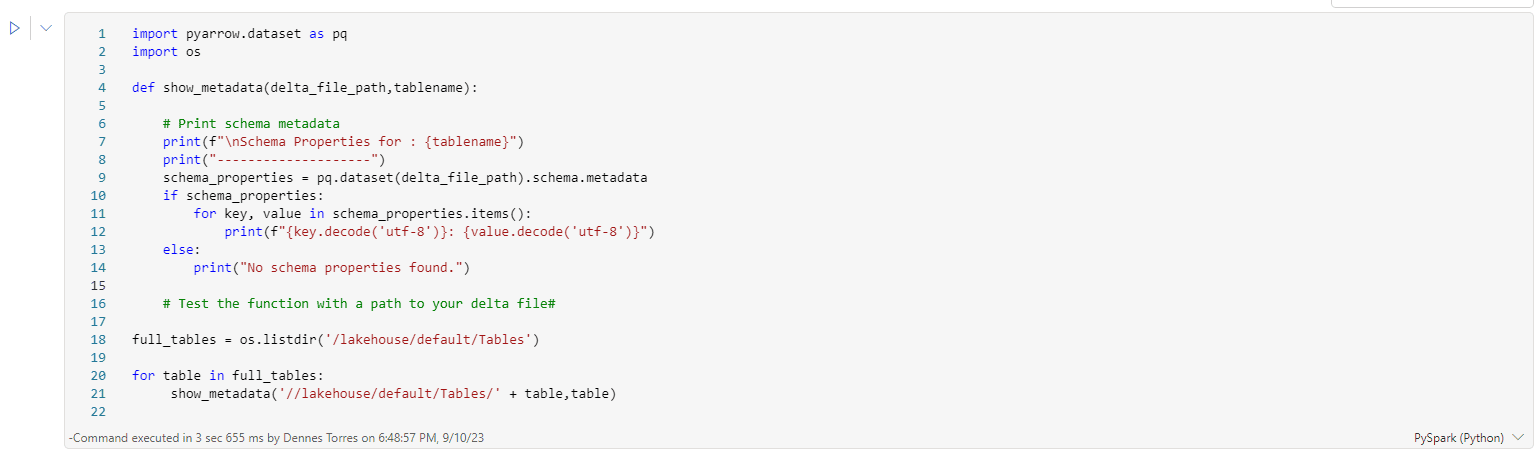
We can use the following PySpark script to check the configuration of the tables in our lakehouse:

import pyarrow.dataset as pq
import os
def show_metadata(delta_file_path,tablename):
 

 # Print schema metadata

 print(f"\nSchema Properties for : {tablename}")

 print("--------------------")

 schema_properties = pq.dataset(delta_file_path).schema.metadata

 if schema_properties:

     for key, value in schema_properties.items():
         print(f"{key.decode('utf-8')}: {value.decode('utf-8')}")

 else:

    print("No schema properties found.")


 # Test the function with a path to your delta file#

full_tables = os.listdir('/lakehouse/default/Tables')

for table in full_tables:
  
  show_metadata('//lakehouse/default/Tables/' + table,table)

A screenshot of a computer Description automatically generated

This script is inspired on a script provided by a user in the Fabric Community forums.

What we should notice about how this code works:

  • We have a procedure defined, called show_metadata.
  • The procedure receives an array of table names as a parameter.
  • In order to generate the array dynamically, we use os.listdir. In this way, the script works for all tables in the lakehouse.
  • The show_metadata procedure is called in a loop for each one of the tables. Mind the standard path for the tables in the lakehouse.
  • Inside the procedure, we generate a dataset and use the properties .schema.metadata to read the properties of the table.
  • We make a loop on the table properties to show each one.
  • The table properties need to be decoded from UTF-8

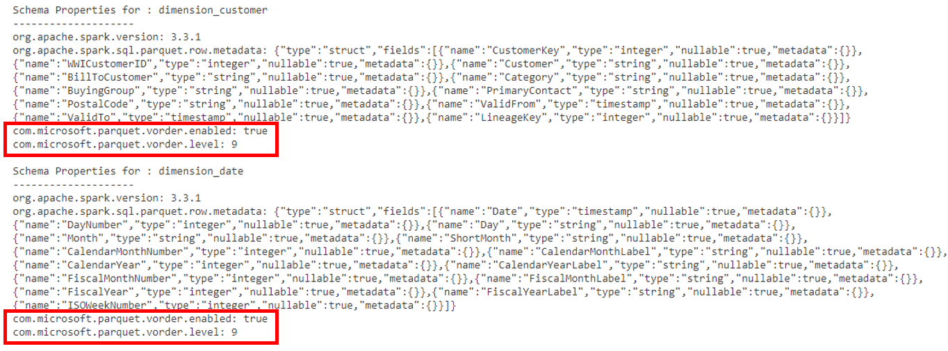
The image below shows a piece of the result after executing this script, highlighting the V-ORDER property on the tables:

A close-up of text Description automatically generated

Using the script to test the configurations

Using this script, we can test the default configuration in different situation, and we will discover the following:

  • The default configuration for spark sessions is to use V-ORDER when writing tables unless we explicitly disable it.
  • This makes the V-ORDER also default when using the Convert-To-Table UI, unless we disable it on workspace levell (Why would we do such thing?)

Fixing a table without V-ORDER

Considering V-ORDER is default on spark sessions in Fabric, it will not be common to have tables not using V-ORDER.

But let’s create one in this situation and discover how to fix it when needed.

If the table dimension_stock_item already exists in your demo environment, you will need to drop it before running this script.

A simple spark SQL statement solves it:

%%sql
drop table dimension_stock_item

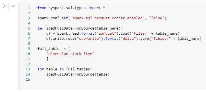
We can use the following pyspark code to create a table without the v-order optimization:

from pyspark.sql.types import *

spark.conf.set("spark.sql.parquet.vorder.enabled", "false")

def loadFullDataFromSource(table_name):

    df = spark.read.format("parquet").load('Files/' + table_name)

    df.write.mode("overwrite").format("delta").save("Tables/" + table_name)

full_tables = [

   'dimension_stock_item'

]

for table in full_tables:

    loadFullDataFromSource(table)

A screenshot of a computer program Description automatically generated

We should mind the following about this pyspark script:

  • We have a loadFullDataFromSource procedure to make the load in a default way. It works unless the table has some specific partitioning.
  • We disable the v-order configuration for the session on the start of the script.
  • We create an array of the tables, but it has only one table. It’s only a standard way to build it.
  • We make a for loop on the array, calling the loadFullDataFromSource procedure. Once again, it’s only a standard way to build it, since in our example it’s only for one table.

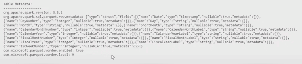
Once the import is executed with the V-ORDER disabled, we can execute again the script to check the Tables metadata and we may notice the lack of V-Order property on this table. The image below illustrates this:

Fixing the lack of V-ORDER

We need to fix this problem without loading the entire table again. In order to do so, we can use the OPTMIZE statement. This statement can reorganize the PARQUET files to avoid the small file size problem and apply the V-ORDER when this one is missing.

It’s very simple:

%%sql
OPTIMIZE dimension_stock_item VORDER;

A white rectangular object with black text Description automatically generated

We can execute the script to check the table’s metadata again and there it is: The table will have the V-ORDER enabled.

A computer screen shot of text Description automatically generated

Disclaimer

On the documentation, the OPTIMIZE is used to reorganize the files and apply the V-ORDER. The ALTER TABLE, also present on the documentation, is used to set a TBLPROPERTY which should ensure future writes in the table use V-ORDER.

TBLPROPERTY seems to have no relation with the metadata extracted by the script illustrated here. The TBLPROPERTY could be set and the metadata not, and the opposite.

Microsoft Fabric is still in preview, many of these details are still going to change and the documentation may not be precise.

Conclusion

All the defaults lead to the V-ORDER always being enabled in lakehouse (data warehouses are a completely different story). But it’s important to be able to check it every time a different scenario appears.


The post Microsoft Fabric: Checking and Fixing Tables V-Order Optimization appeared first on Simple Talk.


from Simple Talk https://ift.tt/cO0y2a3
via

Tuesday, September 19, 2023

Alternatives To SQL-2022 Built-in function GREATEST

If you haven’t already heard, SQL 2022 has introduced a new built-in system function called GREATEST. Simply put, it is to a set of columns, variables, expressions etc. what the MAX function is to a set of values (i.e., rows) of a single column or expression. The opposite of GREATEST function is LEAST function which returns the smallest value from the supplied list of columns, variables, constants etc. GREATEST & LEAST can be considered a pair, just as MIN/MAX functions are.

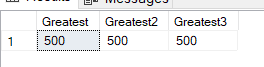
So, on a SQL Server 2022 instance, you can simply call GREATEST function with list of columns, variables, or constant values to get the highest value out of all of them. Here is an example with list of constants:

SELECT GREATEST(500, 10, 3, 50, 200, 8) [Greatest],
       GREATEST(10, 500, 3, 50, 200, 8) [Greatest2],
       GREATEST(200, 10, 3, 50, 500, 8) [Greatest3]

This will return:
A screenshot of a computer Description automatically generated

In the same manner,

I can also pass a list of columns to it:

with cte as
(
select 
      DB_NAME(database_id) db_name,
      max(last_user_seek) last_user_seek,
      max(last_user_scan) last_user_scan,
      max(last_user_lookup) last_user_lookup,
      max(last_user_update) last_user_update
from sys.dm_db_index_usage_stats
group by DB_NAME(database_id)
)
select 
      *,
      GREATEST(last_user_seek, last_user_scan, 
      last_user_lookup,last_user_update) last_access_time_cte
from cte;

This returns the following:

And while it is not as easy to read, note that you can pass in expressions as well, as you can get the same result by pushing the GREATEST function up into the primary query too:

select DB_NAME(database_id) db_name, 
       max(last_user_seek) last_user_seek, 
       max(last_user_scan) last_user_scan, 
       max(last_user_lookup) last_user_lookup, 
       max(last_user_update) last_user_update, 
       GREATEST(max(last_user_seek), 
                max(last_user_scan), 
                max(last_user_lookup), 
                max(last_user_update)) AS last_access_time_cte 
from sys.dm_db_index_usage_stats 
group by DB_NAME(database_id);

Isn’t that a nifty feature?

This rest of this article, focuses on how to achieve the same functionality in pre-SQL Server 2022 versions of SQL Server. Same approaches can be used to mimic the functionality of LEAST function as well.

I recently had to remind a client of mine that we are past the halfway mark of year 2023 that they still didn’t have a single SQL Server 2022 server, even though their SQL Server licenses covered it. I would not be surprised if there are many organizations that may still have a sizable number of SQL Servers pre-SQL 2022.

I personally though, am looking forward to when the next release of SQL Server will come out, whether it would be in 2024, 2025, or 2026? Hopefully Microsoft doesn’t make us wait beyond the year 2026.

In this article I am going to demonstrate 2 viable alternative solutions to find the largest value of a group of values in your queries (not including writing a very complicated CASE expression!)

Table Value Constructor

To start with, I will discuss using a Table Value Constructor (TVC) as I think it is easier to write and understand. TVC is very similar to the VALUES clause that you have used with the INSERT INTO statements to add new data into a table. You are maybe already aware that you can insert multiple rows in a single INSERT INTO statement:

declare @customer table  (id int identity, name varchar(100));
insert into @customer(name)
values
       ('tom'),
       ('jerry'),
       ('brian');
 select * from @customer;

This returns:

id          name
----------- ----------

1           tom
2           jerry

3           brian

Similarly, you can use a VALUES clause to construct a derived table. Here is an example of using it with constants:

SELECT [Greatest] = 
(
    SELECT MAX([Greatest])  FROM
          (VALUES (500),(1000),(3),
                   (50), (200),(8))
             AS derived_table([Greatest])
);

This will return the greatest of values in that derived table:
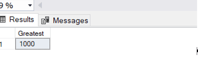
A screenshot of a computer Description automatically generated

Similarly, you can use list of columns, variables, expressions etc. 

So, using the VALUES construct here, I will construct a derived table to convert values from multiple columns into values/rows for a single derived column, last_access_time, sort its results in descending order (from highest to lowest) then select the first row’s value to get the highest (i.e. GREATEST) value.

with cte as
(
select
       DB_NAME(database_id) db_name,
       max(last_user_seek) last_user_seek,
       max(last_user_scan) last_user_scan,
       max(last_user_lookup) last_user_lookup,
       max(last_user_update) last_user_update
from sys.dm_db_index_usage_stats
group by DB_NAME(database_id)
)
select
             *,
             last_access_time_derived = 
                    (select top 1 last_access_time from
                    (values
                           (last_user_seek),
                           (last_user_scan),
                           (last_user_lookup),
                           (last_user_update))
                           derived_table(last_access_time) 
                     order by last_access_time desc
                    )
from cte;

This will return something like the following (depending on your actual server’s utilization):

Note: depending on the kind of server you are using this on, it may have NULL values for some of the values. For example, on the editor’s computer, it returned:

So, just like MAX, it does not return NULL unless all scalar expressions are NULL. This method is by no means as easy to work with as the GREATEST function, but it is generally straightforward to implement if needed.

It looks complicated without the built-in GREATEST function, doesn’t it? Well, I think the next method, UNPIVOT, I will show you is even more complicated. That’s just my opinion, the opinions of others in general may vary.

Unpivot

The idea with using an unpivot is to take values from multiple columns and turns them into rows for a single column. In other words, it can be used to convert a set of columns into a row. If you are familiar with the TRANSPOSE function in excel, unpivot is very similar. It’s the opposite of the PIVOT statement, which takes values for a single column from multiple rows and turns each value into multiple columns.

Here is an example of how you can use UNPIVOT to convert columns into rows (note that if you have not executed any queries in the other databases since a reboot, no data may be returned by this query):

/*
The DMV sys.dm_db_index_usage_stats returns the operational stats on 
each index in every database that have had any read and/or write 
activity since the last restart of the sql instance. It returns 
one row for each index. However, by use of the UNPIVOT clause, I
am converting it's four columns with "last_*" names, into rows so
instead of a single row for each index, it returns multiple rows, 
one row for each column that has a not-null value. 
The where clause filters out:
1. System databases i.e. where database_id > 4
2. Non-clustered indexes i.e where index_id <= 1
   Essentially, when index_id is 0 the table is a heap i.e. 
                                   it has no clustered index
                when index_id is 1 the table has a clustered 
                                       index and is not a heap
*/
SELECT TOP 10
        DB_NAME(database_id) [db_name],
        OBJECT_NAME(object_id, database_id) [object_name],
        [column_name],
        [column_value]
FROM sys.dm_db_index_usage_stats
        UNPIVOT ([column_value]
                     FOR [column_name] IN 
                                (
                                   last_user_seek, 
                                   last_user_scan, 
                                   last_user_lookup, 
                                   last_user_update
                                                )
                ) unpv
WHERE index_id <= 1
AND database_id > 4
ORDER BY [db_name], [object_name], [column_name];

The values for the four columns last_user_lookup, last_user_scan, last_user_seek and last_user_update in the sys.dm_db_index_usage_stats are now showing as rows.
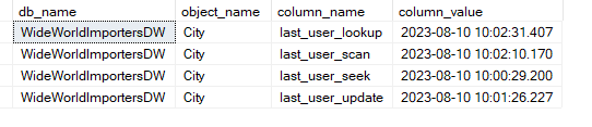
And I just want to know the highest value from the 4 columns, I can just use the MAX function and slightly modify the query to add the GROUP BY clause.

SELECT TOP 10
        DB_NAME(database_id) [db_name],
        OBJECT_NAME(object_id, database_id) [object_name],
        [last_accessed] = MAX([column_value])
FROM sys.dm_db_index_usage_stats
        UNPIVOT ([column_value]
                     FOR [column_name] IN 
                                                (
                                                        last_user_seek, 
                                                        last_user_scan, 
                                                        last_user_lookup, 
                                                        last_user_update
                                                )
                                        ) unpv
WHERE database_id > 4
GROUP BY database_id, object_id
ORDER BY [db_name], [object_name];

This returns the following on my server.
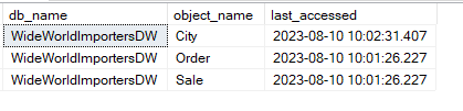
To extend the example further, I want to know if/when the last time a table in the the database was accessed. This query is longer than it may need to be because I also want to display the individual values for the 4 columns as well as the MAX/highest value among them.

USE  MSDB;

with cte as
(
SELECT
        [last_user_seek]   = MAX(last_user_seek),
        [last_user_scan]   = MAX(last_user_scan),
        [last_user_lookup] = MAX(last_user_lookup),
        [last_user_update] = MAX(last_user_update)
FROM sys.dm_db_index_usage_stats AS i
WHERE i.database_id = DB_ID()
)
 SELECT
             [Database] = DB_NAME(),  
             *
FROM cte,
(
       SELECT MAX([last_access_time]) [last_access_time]
       FROM
             (
                 SELECT
                     [last_user_seek]   = MAX(last_user_seek),
                     [last_user_scan]   = MAX(last_user_scan),
                     [last_user_lookup] = MAX(last_user_lookup),
                     [last_user_update] = MAX(last_user_update)
                 FROM cte
             ) p
       UNPIVOT 
             ([last_access_time] FOR [Column] IN
                    (
                      last_user_seek,
                      last_user_scan,
                      last_user_lookup,
                      last_user_update)
                    )  AS unpvt
) unpvt;

This returns:

As you can see, the using UNPIVOT can take more lines of code and can be quite a bit complicated. As you will see later in this article, per the performance test I performed, it is also slower than the Table Value Constructor method.

I have tested these syntaxes in SQL Server versions going back to 2012. PIVOT and UNPIVOT were first introduced in SQL 2005 so the syntax’s I presented in this article should still work there.

Performance Test

How is the query performance between the TVF and Unpivot methods, or with the new greatest function?

To find that out, I am going to generate some random data. The following SQL script creates a table with name random_data_for_testing and inserts 10 million rows into it.

SET NOCOUNT ON;
if object_id('random_data_for_testing', 'U') is not null 
        drop table random_data_for_testing;
GO
create table random_data_for_testing
(
        id int identity primary key,
        value_01 float default substring(cast(rand() 
                              as varchar(20)), 3, 15),
        value_02 float default substring(cast(rand() 
                              as varchar(20)), 3, 15),
        value_03 float default substring(cast(rand() 
                              as varchar(20)), 3, 15),
        value_04 float default substring(cast(rand() 
                              as varchar(20)), 3, 15),
        value_05 float default substring(cast(rand() 
                              as varchar(20)), 3, 15),
        value_06 float default substring(cast(rand() 
                              as varchar(20)), 3, 15),
        value_07 float default substring(cast(rand() 
                              as varchar(20)), 3, 15),
        value_08 float default substring(cast(rand() 
                              as varchar(20)), 3, 15),
        value_09 float default substring(cast(rand() 
                              as varchar(20)), 3, 15),
        value_10 float default substring(cast(rand() 
                              as varchar(20)), 3, 15)
);
GO
declare @commit_size int = 100000; 
declare @max_rows int = 10000000; 
declare @counter int = 1;
declare @commit_counter int = 0;
declare @max_commit_count int = @max_rows / @commit_size; 
while @counter <= @max_rows
begin
        if @@TRANCOUNT = 0 BEGIN TRAN
        
        insert into random_data_for_testing default values
        set @counter = @counter + 1
        IF @@TRANCOUNT > 0 and @counter % @commit_size = 0
        BEGIN
                set @commit_counter = @commit_counter + 1
                raiserror('Committing %i of %i transactions....', 10, 
             1, @commit_counter, @max_commit_count) with nowait
                commit;
        END
end
if @@TRANCOUNT > 0 COMMIT;

My first test query is to do a test to get the highest value among the 10 columns (named value_01 to value_10 in the test table), using all 3 methods. I ran the script multiple times to make sure there are no physical reads or read-ahead reads with any of the queries so we can compare just the duration, logical IO and CPU as accurately as possible.

SET NOCOUNT ON;
SET ANSI_WARNINGS OFF;
GO
PRINT '---------------------------------------------'
PRINT '********* Test using the function Greatest...'
PRINT '---------------------------------------------'
SET STATISTICS IO ON;
SET STATISTICS TIME ON;
GO
SELECT MAX(GREATEST((value_01),(value_02),(value_03),
                     (value_04),(value_05),(value_06), 
                     (value_07),(value_09),(value_10))) 
                                AS using_greatest_function
FROM random_data_for_testing;

SET STATISTICS IO OFF;
SET STATISTICS TIME OFF;
GO
PRINT '---------------------------------------------'
PRINT '********* Test using the TVC method..........'
PRINT '---------------------------------------------'
SET STATISTICS IO ON;
SET STATISTICS TIME ON;
GO
SELECT MAX(greatest_value) using_tvf FROM
(
        SELECT greatest_value = 
                (SELECT MAX(greatest_value) 
                 FROM (VALUES(value_01),(value_02),(value_03),
                             (value_04),(value_05),(value_06),
                             (value_07),(value_09),(value_10)
                                        ) derived_table(greatest_value)
                )
                        FROM random_data_for_testing
) a;

SET STATISTICS IO OFF;
SET STATISTICS TIME OFF;
GO
PRINT '---------------------------------------------'
PRINT '********* Test using the Unpivot...'
PRINT '---------------------------------------------'
SET STATISTICS IO ON;
SET STATISTICS TIME ON;
GO
SELECT MAX(greatest_value) using_unpivot FROM random_data_for_testing
UNPIVOT  ([greatest_value] FOR [Column] IN (value_01, value_02, 
                                            value_03 , value_04, 
                                            value_05,value_06, 
                                            value_07,value_09,
                                                 value_10)) AS unpvt

SET STATISTICS IO OFF;
SET STATISTICS TIME OFF;
GO

Results:
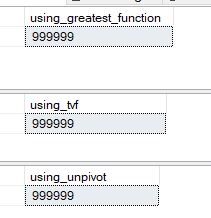
Here are the key stats from the STATISTICS IO and STATISTICS TIME:

********* Test using the function Greatest...
Table 'random_data_for_testing'. Scan count 5, logical reads 118295
SQL Server Execution Times:
CPU time = 4405 ms, elapsed time = 1381 ms.

********* Test using the TVC method..........
Table 'random_data_for_testing'. Scan count 5, logical reads 117343
SQL Server Execution Times:
CPU time = 12000 ms, elapsed time = 3332 ms.

********* Test using the Unpivot...
Table 'random_data_for_testing'Scan count 5, logical reads 117179
SQL Server Execution Times:
CPU time = 17219 ms, elapsed time = 4813 ms.

The amount of IO (logical reads) is almost identical among the three methods. But notice the difference in the CPU time and Elapsed time values for each. The elapsed time for the function GREATEST is 1381 ms, for the TVC it is 3332 ms and for UNPIVOT it is 4813 ms.

Below is the screenshot of the actual execution plan and as you can see the query cost as relative to the batch, cost of function GREATEST is 12%, TVC is 34% and the UNPIVOT is 54%.
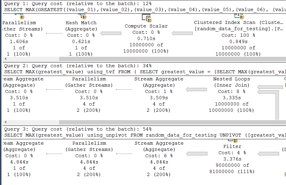
As you can see from the thickness of the pipe going from right to left, when a query needs to process a relatively great deal of rows, using the build in function gives the best performance. That shouldn’t be a surprise. If that wasn’t the case, somebody at Microsoft made a big booboo! However, between the TVF and Unpivot, TVF is faster.

Note: This by no means a scientific test. Generally, though I have seen TVF to be faster than Unpivot.

What if the query is using a very selective filter condition on a clustered primary key on a single, integer column? This kind of queries are usually ideal queries in “almost” any conditions, even if it includes columns with LOB data types like XML, VARBINARY(MAX) etc.
Just to be sure, let’s look at the following example:

SET NOCOUNT ON; 
SET ANSI_WARNINGS OFF; 
GO 

declare @id int = 100100; 
PRINT '---------------------------------------------'; 
PRINT '********* Test using the function Greatest...'; 
PRINT '---------------------------------------------';
SET STATISTICS IO ON; 
SET STATISTICS TIME ON;

SELECT *,
        using_greatest_function = 
                          GREATEST(value_01,value_02,value_03,value_04, 
                                   value_05,value_06,value_07,value_08,
                                   value_09, value_10                                                   ) 
FROM random_data_for_testing 
WHERE id = @id;

SET STATISTICS IO OFF; 
SET STATISTICS TIME OFF; 
PRINT '---------------------------------------------' 
PRINT '********* Test using the TVC method..........' 
PRINT '---------------------------------------------'

SET STATISTICS IO ON; 
SET STATISTICS TIME ON;  

SELECT  *, using_tvf = ( 
                SELECT MAX(greatest_value) 
                FROM  (VALUES (value_01),(value_02),(value_03), 
                              (value_04),(value_05),(value_06),  
                              (value_07),(value_08),(value_09),                           
                              (value_10)) AS derived_table(greatest_value)                       ) 
FROM random_data_for_testing 
WHERE id = @id;

SET STATISTICS IO OFF; 
SET STATISTICS TIME OFF; 

PRINT '---------------------------------------------'; 
PRINT '********* Test using the Unpivot...'; 
PRINT '---------------------------------------------';
SET STATISTICS IO ON; 
SET STATISTICS TIME ON; 

SELECT t.*, p.using_unpivot 
FROM random_data_for_testing t
        INNER JOIN  ( SELECT id, MAX(greatest_value) using_unpivot 
                      FROM random_data_for_testing 
                      UNPIVOT  ([greatest_value] FOR [Column] IN  
                                  (value_01,value_02,value_03, value_04, 
                                   value_05, value_06, value_07, value_08,
                                   value_09, value_10)) AS unpvt 
                       WHERE id = @id group by id ) p 
               on p.id = t.id;

SET STATISTICS IO OFF; 
SET STATISTICS TIME OFF;

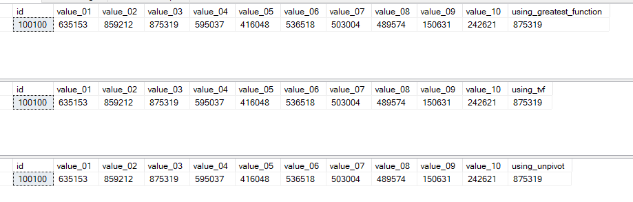
This returns three identical result sets:
And quite similar execution times as well:

********* Test using the function Greatest...
Table 'random_data_for_testing'. Scan count 0, logical reads 3
SQL Server Execution Times:
CPU time = 0 ms, elapsed time = 0 ms.

********* Test using the TVC method..........
Table 'random_data_for_testing'. Scan count 0, logical reads 3
SQL Server Execution Times:
CPU time = 0 ms, elapsed time = 0 ms.

********* Test using the Unpivot...
Table 'random_data_for_testing'. Scan count 0, logical reads 6
SQL Server Execution Times:
CPU time = 0 ms, elapsed time = 5 ms.

With the following actual execution plans:
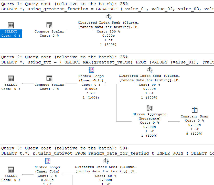
The entire script finishes in sub-sub-second. Still, at a microsecond (a millionth of a second) level, you can see that the Unpivot performs the worst.

Summary

In this article, I have demonstrated the new GREATEST and LEAST value functions in SQL Server 2022 and have show that in general testing, these functions are very fast. However, as not everyone is using SQL Server 2022, I also demonstrated a method using Table Value Constructors that give you similar functionality (with much less straightforward code), as well as a method using the often disregarded UNPIVOT function.


The post Alternatives To SQL-2022 Built-in function GREATEST appeared first on Simple Talk.


from Simple Talk https://ift.tt/MeO7CUY
via
Monday, September 18, 2023

SQL Server Row Level Security Deep Dive. Part 4 – Integration, Anti-patterns, and Alternatives

One of the primary reasons to implement RLS is to facilitate reporting and ease the administrative burden. This section covers some considerations for using RLS with the primary Microsoft reporting engines and gives you an idea of things to look for in your reporting engine. Some anti patterns and alternatives to RLS are also examined.

Power BI

Power BI integrates directly with RLS when using direct query access. Most department level implementations of Power BI will likely use the built in caching, which makes performance tuning much easier. In larger enterprise level implementations of Power BI, RLS may fit the requirements. Nothing special is needed to integrate it with Power BI, other than direct queries.

RLS is also available as a separate mechanism in Power BI. This allows data cached by Power BI to also be controlled by RLS. If RLS is used in the database tier, it must also be implemented in the Power BI tier when using caching. This results in a redundant implementation, but data is protected at all levels. It also allows the caching benefits of Power BI to be used while still using RLS.

It is recommended to use the same RLS rules in both the database and Power BI. This will reduce the amount of troubleshooting and ensures the business requirements are met. This is a good thing to keep in mind when designing your RLS implementation. Business users won’t understand the architectural implications of a design, so it is your job to help this as much as possible. Even less technical users on the team or those not as familiar with SQL and RLS will need guidance. A simple design that meets the requirements is usually the best design choice.

SQL Server Reporting Services (SSRS)

SSRS connections using pass through authentication to SQL Server use RLS seamlessly. SSRS has internal caching mechanisms in the SSRS temp database, but it doesn’t impact the data returned to users, unlike the Power BI caching mechanism. As with all uses of RLS, any type of access to the data is protected when hitting it via SSRS. If the connection string for a report uses a service account, it will not be protected by RLS. To be more precise, it will be protected by RLS, but all users of the report will have the same access and that access will correspond to the authorization of the service account.

Application Integration

It is generally a bad idea to have users directly access transactional systems, but applications are able to use RLS via a few different methods. The SESSION_CONTEXT can be set or a specific user can be designated using EXECUTE AS USER syntax. This is one of the methods used in the WideWorldImporters sample. Using RLS for application security can simplify some development tasks, but may not be worth the extra effort. If your application requires additional layers of security, such as screen level access or if on-screen functionality differs depending on the current user, adding RLS may be redundant. If the application is simple and requires immediate access to data for reports, RLS may fit the need. If used in a transactional system, be sure to test scenarios for administrators and service accounts for your API layer. Performance tuning is important for any RLS application, but it becomes critical for user facing applications.

General considerations

Service accounts with elevated access bypass RLS for report users. In this scenario, users have the same access as the service account. This can be a feature or a bug depending on your implementation. This is related to the caution about cached data. Cached data used by some report engines will effectively bypass RLS if a service account is used. There are generally additional security mechanisms in these report engines that allow user access to be controlled, but it must be considered. Testing should include report access for different users and database level access if appropriate.

Anti Patterns

There are instances when RLS isn’t a good choice for a project. This will vary, and there are always exceptions, but if you find yourself using RLS with one of the following patterns you should stop and consider if it is the correct choice. When working outside of normal patterns it is always a good idea to have enough reasons to be able to defend your decisions.

Transactional systems

Direct user access to transactional systems is a poor choice in most scenarios. Using RLS doesn’t change this pattern. Potential issues with blocking, untested queries, excessive I/O and CPU, security concerns, extra exposure to the database are all potential issues.

RLS can be used in transactional systems without granting direct access to the system. This can be used as a way to implement restricted security without much of the custom coding typically associated with restricted access. It depends on the specific business needs, but an API layer can set the executing user via SESSION_CONTEXT() and as a consequence, different rows can be returned. This wouldn’t work for all scenarios and would start to get more complicated as actual pages or functionality needs to be restricted, but it’s an interesting pattern. An example of this is given in the WideWorldImporters sample database and associated code.

Databases without direct user access

Databases that don’t allow direct user access aren’t likely candidates for RLS, since the whole point of row level security is direct access control. There are patterns for RLS that would work in these scenarios, but they are generally managed at an API level.

Less experienced teams

Setup and long-term maintenance and troubleshooting can be challenging with RLS. Teams that are inexperienced with SQL Server may not be a good choice for implementing RLS. All teams can be trained, but there are some teams that focus on development or business groups that also manage a database. There isn’t a checklist to determine if a team can manage RLS, but experience of the team and available support after implementation are key factors in the decision process.

Multi-tenant systems

I would recommend against using RLS as the security mechanism for multi-tenant transactional client systems. Access for these systems will generally not be direct data level authorization. If users are allowed to directly query the data, they can impact the performance of other clients. If implemented properly (no direct access and no ad-hoc queries), data won’t be exposed, but it does make maintenance and administration more difficult.

Data warehouses used by multiple affiliated departments or groups work well with RLS and are generally more tolerant of potential issues. Typically, reporting and ad-hoc queries are also less sensitive to performance variations. Properly modeled data also helps with performance. The table design can take RLS into account and include the RLS columns in the base design, greatly decreasing performance impacts. Take special care with security and consider additional audits if the data is especially sensitive.

Considering the potential for side-channel attacks, I wouldn’t recommend RLS for direct access with multiple external clients, even in a data warehouse scenario. If you do go down this path, be sure contracts support this and clients are aware, as some require separate physical servers with no chance of errors.

Staging / load databases

Staging or load databases are a common ETL pattern. A staging database is used to house data as it is prepared for the final warehouse. It is a landing zone where data can be manipulated and analyzed before it hits the production system. The same functionality can be achieved with schemas and locked down security in the production database, but a staging database offers some advantages. The entire database can be locked down to include only developers and the ETL service account, backups in the primary system will be smaller, performance can be tuned separately for each database (i.e., separate tiers in Azure or separate drives on a physical server), and no RLS is needed at this layer if users are properly restricted. This can ease the performance load involved with ETL, help testing, make reloads easier, and improve data analysis and profiling without impacting production data. There are almost no scenarios where end users would be allowed access to the staging database. The data in staging databases, or even just staging tables, tends to have more chaotic data. This data may not be curated to the degree necessary to implement RLS. RLS is not a good fit for staging databases. It isn’t even a good fit for staging tables. These databases or staging tables should be excluded from direct user access. Only ETL service accounts, developers and testers need access to these database objects. RLS requires extra work, configuration and testing. Removing that requirement for a load process can reduce the number of errors in the development process and during loads. When service accounts are changed it is easy to have ETL scenarios resulting in duplicates, excess deletes, or general errors. Having a locked-down zone without this requirement makes each part of the process easier.

Other databases or systems that don’t need RLS

SQL Server has robust security structures and mechanisms with great flexibility. Standard security structures and design should be considered first. In fact, security requirements are a first part of any SQL database design and should be considered at each step of the process and with each business requirement. The standard security structures, such as system roles, application roles, schema level security, execute as, etc. should all be evaluated and applied to meet requirements first. They require virtually no coding and minimal testing after initial setup and validation. Programming objects such as stored procedures, views and functions can also be used as a security layer, but they do require more testing and maintenance.

Small user base

Systems with a small user base likely don’t require RLS to keep them secure. There are some exceptions, but small systems should be kept uncomplicated when possible. A simple view layer or stored procedures usually will meet the needs of these systems. Smaller systems generally mean smaller support systems and that should be accounted for in the design.

There are multiple ways to bypass the need for RLS. Some are easier than others, but most are more administrative or developer intensive than using RLS. Whenever choosing a solution, it’s always a good idea to at least consider other options. I include this advice for all database design decisions down to the level of a single column definition. You should be able to defend each choice in a database design and RLS is no different. Considering the security and performance implications and the development overhead, it is especially true for RLS. This isn’t an inclusive list of alternatives, but some common solutions.

Alternatives to RLS

There are multiple ways to bypass the need for RLS. Some are easier than others, but most are more administrative or developer intensive than using RLS. Whenever choosing a solution, it’s always a good idea to at least consider other options. I include this advice for all database design decisions down to the level of a single column definition. You should be able to defend each choice in a database design and RLS is no different. Considering the security implications and the development overhead, it is especially true for RLS. This isn’t an inclusive list of alternatives, but some common solutions.

Multiple databases

 For multiple clients or user groups, creating a separate database for each client can be a viable option. Separate databases can be an especially tempting method when there are regulatory issues involved or if data is stored for competing companies. Care must still be taken with this method. In a server environment, it is easy for a single login to access multiple databases. Administrators of multi-tenant systems should be familiar with the security considerations for their particular system. Additional and regular audits are recommended to ensure everything is configured correctly.

Creating a separate database for each group or set of users requiring access can be a tedious process and difficult to maintain. Objects need to be synchronized, bugs found in one database likely impact the other databases, performance related issues need to be synchronized, users need to be maintained, and all administrative tasks need to be configured. Patterns and templates should be established for creating new databases, objects, and maintenance tasks. DevOps deployments with a common code base also make this easier.

Devops

A database project deployed via standard DevOps methods is recommended to keep multiple databases with the same objects synchronized. This includes objects such as indexes and constraint names. It is common in projects with duplicated databases for different clients to have custom objects in each database. These should also be managed in a database project, allowing for automatic deployments. Separate branches or even projects can be used for these customizations. Whatever method is used to maintain each database, consistency is critical. Methods need to be created to synchronize not only objects, but to maintain users, configure administrative tasks and possibly implement maintenance tasks.

Multiple reports

Another method to provide different data based on users is to create different queries and reports for each distinct set of users. This offers some simplicity in the initial design, but long-term maintenance can be more complicated or at least tedious. This is a very straight-forward solution that is easily understood by less-technical members of the team. Once a base report is designed, it is very simple to copy that report and change the items specific to a group of users.

If using this design pattern for your project, there are a few things that need to be addressed. The primary concern is how to replicate or copy reports and keep them synchronized. The initial creation of reports is relatively easy, but future changes are the challenge. It is easy to put a rule in place that all reports in a group must be updated at the same time, but harder to ensure that it happens. I don’t have a great solution for this problem. Development can be chaotic, especially when there are team changes or when a high-priority bug is fixed. Anyone with data experience knows that some issues only happen with particular sets of data. They might be outliers or they might be errors. In a critical situation, the group of users, meaning one particular report, will be fixed first. Ideally the other reports based on the same template should then be updated, but it may not always happen. Code reviews, automated tools and testing are the common ways to manage this.

The next item for copied reports is determining the testing strategy. A testing strategy is needed for all development tasks, but this one can be deceptively difficult. The assumption might be that all reports based on the same core report are the same other than some WHERE clauses. But there is no guarantee that all reports are synchronized, so a thorough testing pattern must be established. There are some programmatic methods to decrease this burden, but those methods must be created and followed for every report. This can include creating a template for each group of reports or doing a diff on each group of reports. But an extreme amount of rigor must be employed in development to allow testing shortcuts. It can be useful to bring the test team into the conversation early in the development phases to ensure their requirements are considered.

Another consideration for creating multiple reports is the method for exposing those reports to end users and general organization. This depends on the report engine or custom method for creating reports. This also can be the primary method for securing the data, so be sure the method you choose is correct for your architecture.

Custom code in SQL 

SQL Server objects are a very common method for restricting access to data and are often considered a security mechanism when used in this way. Almost any SQL object can be used in this way. Common methods are listed below.

Stored procedure logic

Only allowing access to data through stored procedures is a common security mechanism for direct SQL access. Any logic check or lookup can be performed in the stored procedure. It is also possible to create different stored procedures for different groups of users. If groups of stored procedures are used to limit access, you will want to organize those procedures in a way that makes it easier to manage them. Creating a schema for each group and creating procedures in those schemas greatly simplifies the management. This approach can also be layered with the reporting strategy so that each report for a particular group hits different stored procedures in their designated schema.

Views

Creating different views for groups of users is another effective way to control access to data. As with stored procedures, it is useful to group views in some way. Naming conventions or different schemas are both useful. I like to create a different schema for specific users or groups. This simplifies administration greatly since I only need to apply security to the schema. This also makes is easy to tell what is happening in the database just by looking at the schemas. Views can be combined with stored procedures and used by the reporting layer.

Triggers

Triggers can’t be used with SELECT statements, but they can be used to control INSERT, UPDATE, and DELETE statements. They can also be used with views using the INSTEAD OF option. The use case for this is likely small, but it’s worth considering if DML (INSERT, UPDATE, DELETE) is needed with the solution. An INSTEAD OF trigger can be combined with stored procedures or views to manage the SELECT portion of the requirements.

This isn’t a solution I would focus on developing and is an anti-pattern. A more robust solution is to focus on automating ETL processes and eliminating the need for direct user updates.

Scalar Functions / Table Valued Functions

Functions, both scalar and TVF can be used to limit the data returned to users. On the surface, this can be a tempting pattern. You could create a function that limits data in a way similar to RLS and use it in all of your stored procedures. If you only allow access via stored procedures, data is locked down and it is a simpler solution than RLS.

The main issue with this design pattern is that functions have a tendency to be performance killers. You might encounter hidden RBAR (row-by-agonizing-row), which is similar to a hidden cursor. Using a scalar function is generally tied to using it in the WHERE clause or in a JOIN. This also causes performance issues. This alone is a good enough reason to avoid functions. Security misconfigurations are also a possibility and are discussed in the next section.

Disadvantages of Custom Code

Even though it must be tested and validated, an advantage of RLS is that it is within a standard framework and portions of it can be validated with data management views (DMV). RLS is non-prescriptive, but there are requirements that must be met to implement RLS. And you will generally follow a standard pattern for RLS within a database project. This allows automated validation and makes it easier to perform code reviews and object validation.

This is in contrast to custom code. As with RLS, it must be tested thoroughly, but there aren’t generic patterns that can be discussed. It all depends on the individual implementation. There will be standards that are followed, but each user group will have a different set of criteria. This makes it challenging to automate validation.

As mentioned, custom code must be tested extensively. Since new objects are created for each user group, the coding and testing effort can be extensive. Not only does each new object or report need to be tested, each group added also creates a set of database objects or reports that need validation. This adds a maintenance burden to the developer team and to the test team.

Performance must be carefully managed when using custom code. This is no different from any solution, including RLS, but there are some methods that might appear tempting to use that can cause issues. If generic objects are created to manage access and ease management, especially functions, they can cause hidden RBAR in the query plan.

Another potential issue is related to misconfigurations. This is subjective, but I think there is a greater chance of security gaps when using custom objects than with RLS. If security administrators aren’t aware of the custom code strategy getting used, they could grant direct access to tables using db_datareader. This would allow users to bypass the SQL objects. I have seen administrators try to troubleshoot RLS issues by granting db_datareader and even db_owner role access. With RLS, no extra data is returned. With SQL objects, this type of misconfiguration leads to all data getting exposed.

The other thing to keep in mind is that users often find a way around limitations. If data is so restricted that users don’t use the system, they will probably find the data in another system or use an extract. This can actually make the overall system less secure. Discuss needs with users and make sure the solution works for users while still keeping the data secure.

Application logic

Letting an application control access to the data is the standard pattern for modern architectures, so this isn’t much of an alternative. It is probably more realistic to call RLS the alternative to this pattern, but it is included here for the sake of completeness. There are many ways that applications control access to data. For larger enterprise applications, this is usually table-based controls, security groups, or token-based access of some type. If users don’t need direct access to the database, this is usually a safe choice.

Summary

RLS is a great solution for some projects, but previous methods for differentiating access might be a better fit for some projects. Any method selected, including RLS, need to be thoroughly tested and the code needs to be managed. Each method has challenges and the specific needs of the project will dictate what is needed. Usually there are multiple viable options and the general technical stack used and team skills will be a big driver of what is implemented.

RLS seamlessly integrates with most report engines with some caveats. It is still the responsibility of the development team to ensure that data is protected if external teams and report engines access the data. The primary concern with external access is caching and sharing of data that effectively bypass RLS if the same standards aren’t enforced. Replicating RLS in the destination system or locking down the data to authorized users are common ways to enforce security in any destination system.

RLS doesn’t fit all scenarios and there is a fair amount of administrative overhead in the design, implementation, and maintenance of RLS. It may not fit transactional systems, staging databases, small systems or systems without administrative support. Security and proper database design should take these factors into consideration.

Next sections on RLS:

Part 5 – RLS Attacks

Part 6 – Mitigations to RLS Attacks


The post SQL Server Row Level Security Deep Dive. Part 4 – Integration, Anti-patterns, and Alternatives appeared first on Simple Talk.


from Simple Talk https://ift.tt/1sCtvrw
via

Saturday, September 16, 2023

How to Set up Jenkins CI/CD on Kubernetes Cluster using Helm

Jenkins is an open-source multi-platform software for continuous integration/continuous delivery and deployment (CI/CD) in DevOps. It is one of the most common CI/CD tools. Jenkins uses CI/CD pipelines to automate the software development and deployment workflows. Jenkins uses plugins to integrate with DevOps tools such as Docker and Kubernetes.

Jenkins plugins can also be used to integrate with cloud providers such as Google Cloud, AWS, and Microsoft Azure. If you want to integrate any DevOps tool with Jenkins, you have to install its plugin in the Jenkins controller platform. In this tutorial, you will learn how to set up Jenkins CI/CD on Kubernetes Cluster using Helm. Helm is one of the easiest ways of installing an application on the Kubernetes Cluster.

Prerequisites

For you to follow this tutorial on how to Setup Jenkins CI/CD on Kubernetes Cluster using Helm, you must:

  • Have Docker set up and understand how to use Docker:
  • Understand Kubernetes. (There is some free training on the Kubernetes site)

How to Setup Jenkins CI/CD on Kubernetes Cluster using Helm

Helm is an open-source platform that was created by DeisLabs. Helm is used as the package manager for Kubernetes. Many developers use Helm to install any Kubernetes application to the Kubernetes Cluster. Helm automates the process of deploying a Kubernetes application to the Kubernetes Cluster. Helms bundles a Kubernetes application into a single package known as a Helm chart. Developers will then take this Helm chart and install them on the Kubernetes Cluster.

A Helm chart contains all the Kubernetes YAML files for deploying a Kubernetes application. Once you install the Helm chart on the Kubernetes Cluster, it will create the Kubernetes components such as Kubernetes Deployment and Service on the Kubernetes cluster. You can create your Helm chart using Helm or you can reuse other people’s Helm charts.

Helm has an official Helm Chart repository called ArtifactHub] where developers can push and publish their Helm Charts. In this repository, you can easily find Helm charts for any Kubernetes application and reuse them. For complex applications like Jenkins, it is best to use the official Jenkins Helm Chart. Many Developers have contributed to the Jenkins Helm chart and it has all the Kubernetes YAML files. It will save us time in creating our custom Jenkins Helm chart. In this tutorial you will search and download the official Jenkins Helm Chart from ArtifactHub. We will then install the official Jenkins Helm Chart on the Kubernetes Cluster using Helm. Let’s install Helm.

Installing Helm

There are several ways to install Helm which are covered in the official Helm installation guide. You can check out the official Helm installation docs here. In this article, we will cover the online way, but there are other ways to install it.

Helm is a package manager for Kubernetes that makes it easy to install and manage Helm charts. A Helm chart is a collection of Kubernetes resources that can be used to deploy an application or service.

Before you install Helm, you must configure/create a Kubernetes Cluster. We will install Helm on the configured Kubernetes Cluster. There are various Kubernetes Kubernetes Clusters that you can configure. You can check out here the different types of Kubernetes Cluster. Cloud providers like Google Cloud, AWS, and Microsoft Azure have a dedicated Kubernetes Cluster that you can configure and use. In this tutorial, we will not use any of the cloud providers, instead, we will use a local Kubernetes called Minikube that comes with Docker. As long as you have Docker running you can easily configure Minikube. To configure and start Minikube, follow these steps:

Start Docker

Once you have started Docker, it is now easy to start Minikube.

Configure and start Minikube

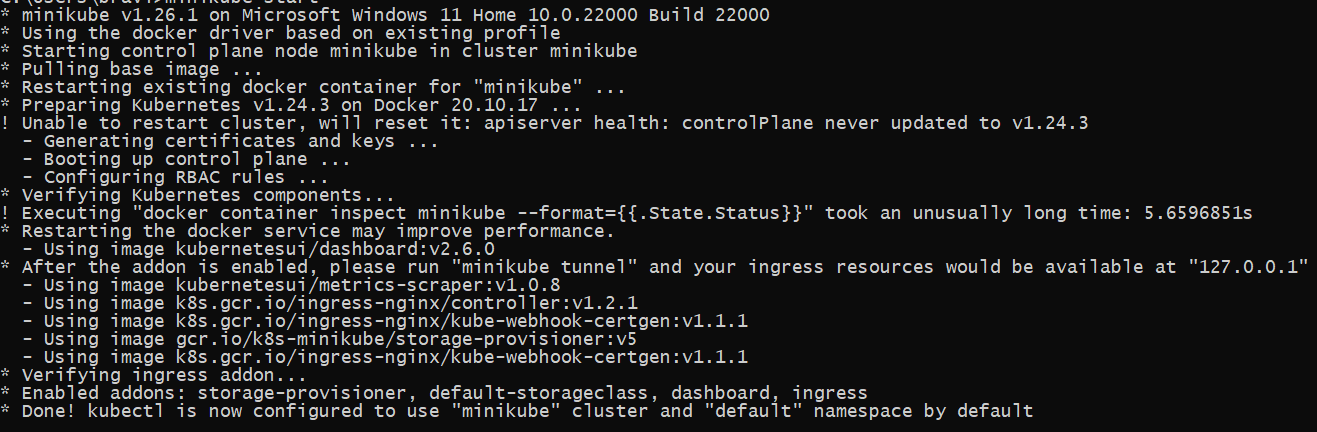
To configure and start Minikube, run this command in your shell:

minikube start

The output should be similar to:

Now that we have configured and started our Kubernetes Cluster (Minikube), let’s install Helm. There are different ways of installing Helm on your specific operating system. There are other ways of installing Helm on your machine. In this tutorial I will show you how to install Helm on Linux, macOS, and Windows.

You can go through the official Helm installation guide to see the other ways of installing Helm on your specific machine.

Installing Helm on Linux

To install Helm on Linux, open your Linux terminal and execute this command:

sudo apt-get install helm

Installing Helm on Windows

To install Helm on Windows, open your Git bash terminal and execute this command:

choco install kubernetes-helm

Installing Helm on macOs

To install Helm on macOs, open your terminal and execute this command

brew install helm

Helm Installation Output

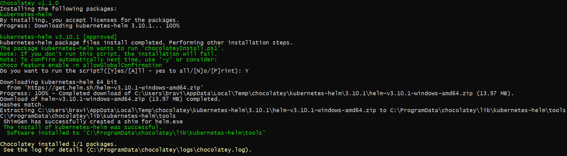
I have installed Helm on my Windows operating system as shown in the image below:

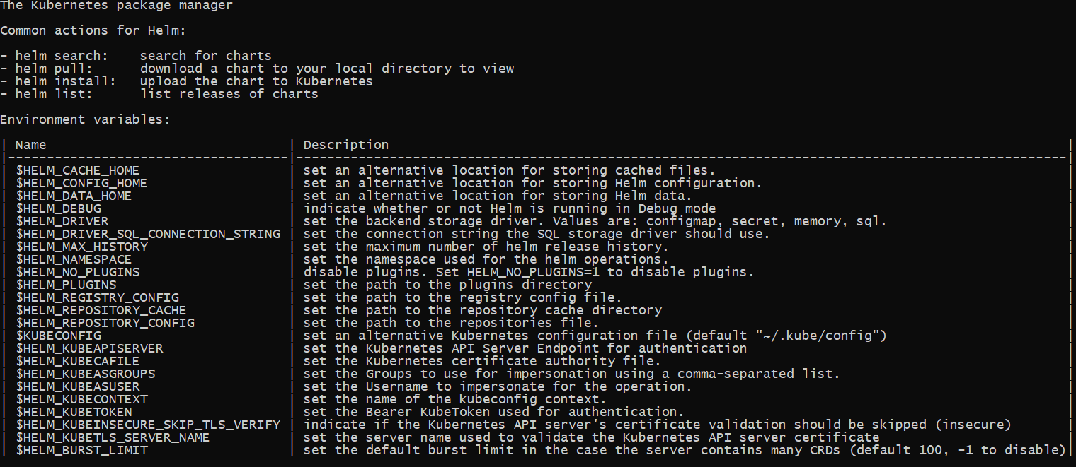
To check if Helm is running in your Kubernetes cluster, run this in your shell in your shell:

helm

The command should output the following in your terminal:

After you have installed Helm on your specific operating system, the next step is to search for the official Jenkins Helm Chart on the ArtifactHub.

Searching for the Official Jenkins Helm Chart

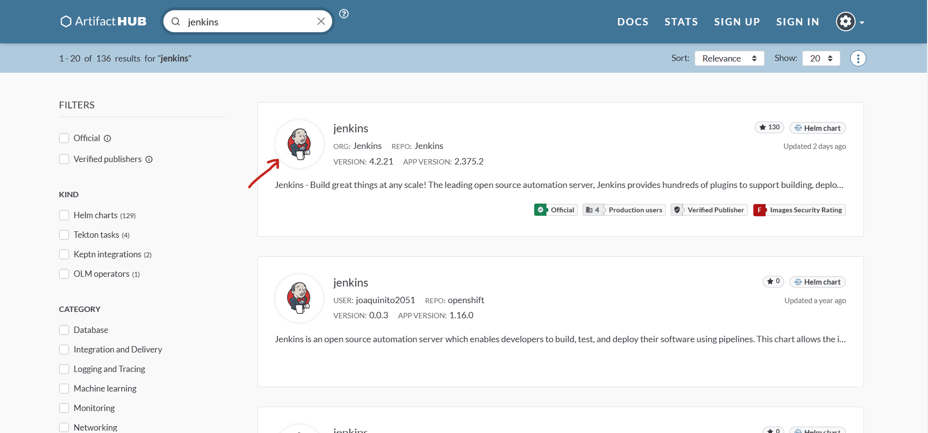
You will search the official Jenkins Helm chart on ArtifactHub. ArtifactHub is a web-based application that enables finding, installing, and publishing Helm charts.

You can click on this link https://artifacthub.io/ to open ArtifactHub.

You can then search for Jenkins Helm Chart as shown below:

After finding the official Jenkins Helm Chart on ArtifactHub, you need to add the Jenkins chart repository on your local machine.

To add the Jenkins chart repository on your local machine, run this command in your shell:

helm repo add jenkins https://charts.jenkins.io

It will download and add the official Jenkins Helm Chart repository. To update this repository and get the latest version of the Helm Chart, run this command in your terminal:

helm repo update

This command will get the latest version of Jenkins Helm Chart by default. For more information, go here:

Installing the Official Jenkins Helm Chart on the Kubernetes Cluster using Helm

Step One: Run this command in your shell

helm install myjenkins jenkins/jenkins

This command will deploy the Jenkins CI/CD on the Kubernetes cluster. The name of the Jenkins Helm Chart release is myjenkins. There are different versions and releases for the Jenkins Helm chart that you can use. In this article you will use myjenkins since it is the release that has all the configurations for running the CI/CD pipeline.

Helm will use the Kubernetes YAML files in the Helm and create the Kubernetes components (Deployment and Service). We have reused the official Jenkins Helm Chart to set up the Jenkins CI/CD on the Kubernetes Cluster.

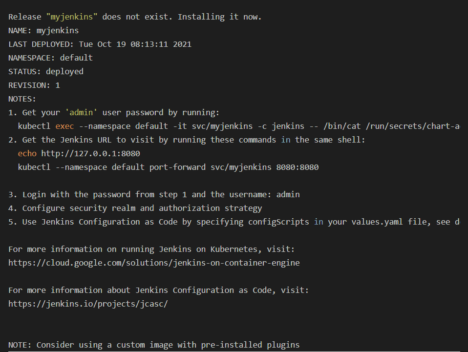
Output is shown in the image below:

To start using the Jenkins CI/CD running on the Kubernetes Cluster, follow these steps:

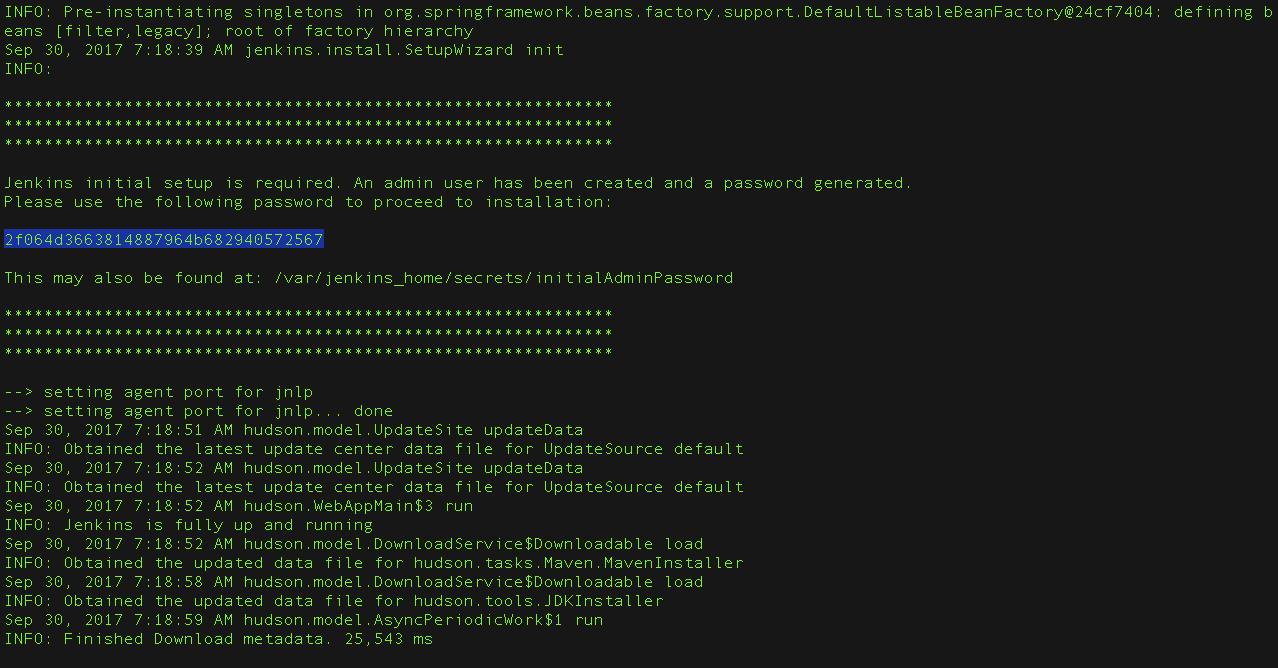
Step Two: Get your ‘admin’ password for Unlocking Jenkins

To get the admin password, run this command in your terminal. You have to execute the first command found in the output above to get the admin password.

kubectl exec --namespace default -it svc/myjenkins -c jenkins – 
/bin/cat /run/secrets/chart-admin-password && echo

Admin Password Output:

Step Three: Get the Jenkins URL

To get the Jenkins URL, run the following shell command:

kubectl --namespace default port-forward svc/myjenkins 8080:8080

Output:

This command will expose the Jenkins container instance on port 8080. You can go to http://127.0.0.1:8080 to access the Jenkins CI/CD

Step Four: Unlock Jenkins with Admin Password

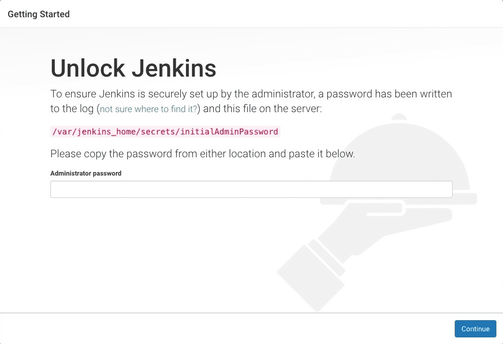
To unlock Jenkins with an admin password, open http://127.0.0.1:8080 in your browser to access your running Jenkins container instance as shown in the image below:

Copy the initial administrator password and paste it into the password field. It will unlock the running Jenkins container instance. You can now finish setting up Jenkins.

Step Five: Finishing setting up Jenkins CI/CD

To finish setting up Jenkins CI/CD follow these steps:

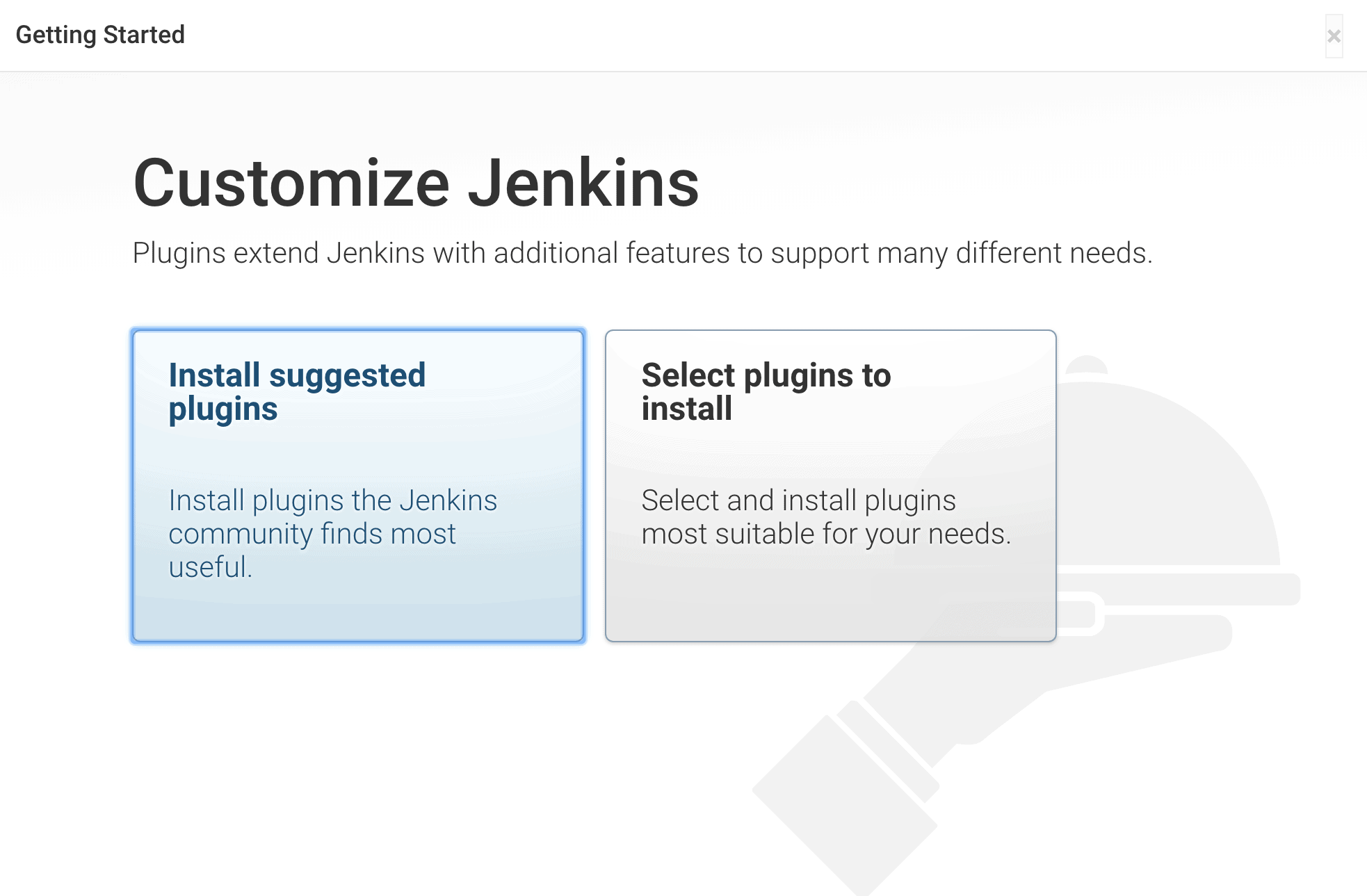
Customize Jenkins

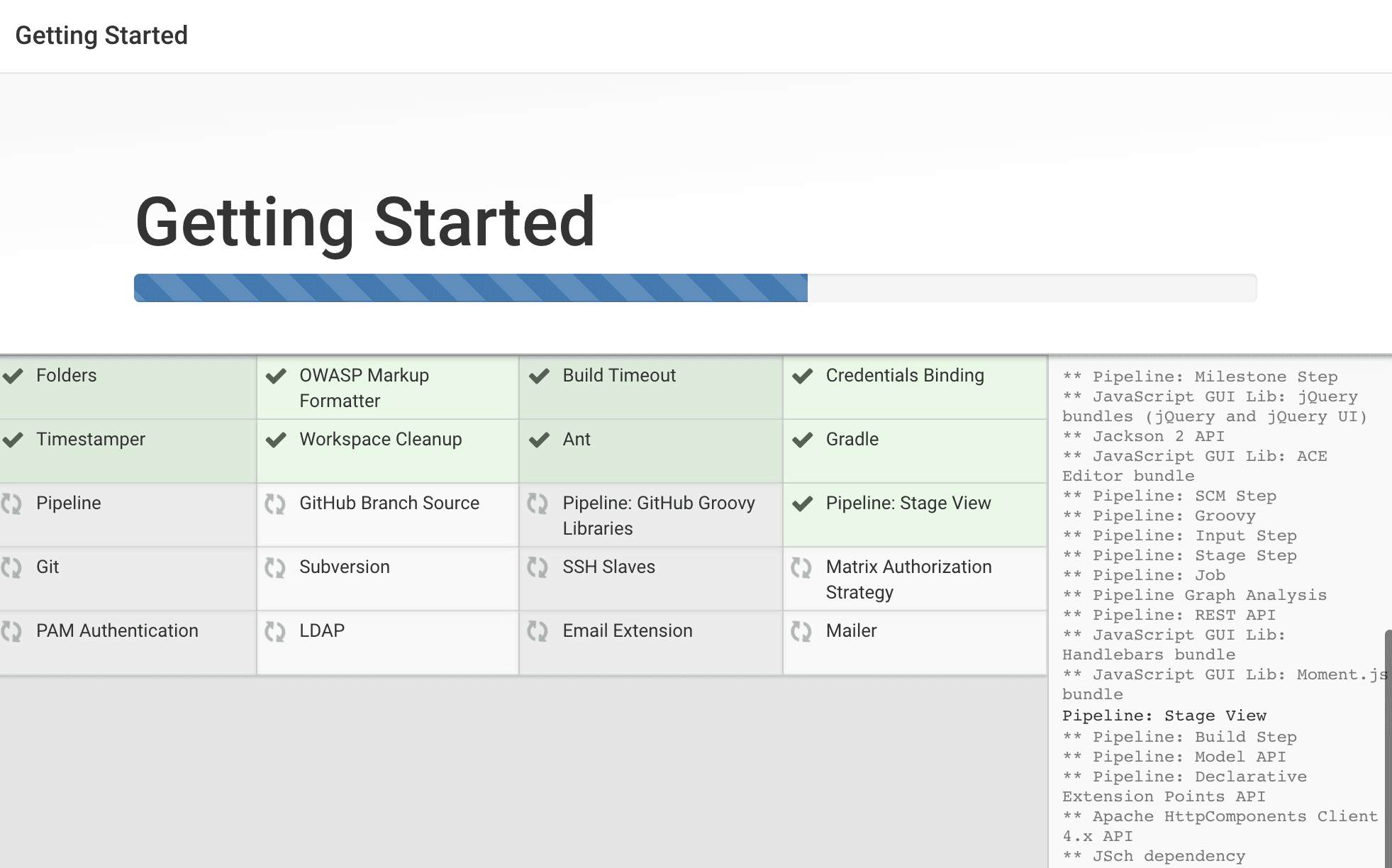
You will install the suggested plugins to customize Jenkins as shown in the image below. Select Install suggested plugins to allow the installation of the necessary plugins. The plugins to be installed are shown in the image below:

After a few minutes (depending on your internet speed), it will install the suggested plugins. This step will install plugins such as:

  • Git Plugin
  • Blue Ocean
  • Simple Theme
  • Performance Publisher
  • Dashboard View
  • Maven Integration
  • Folders
  • Bootstrapped-multi-test-results-report
  • Pipeline Utility Steps

These are the basic plugins that Jenkins requires to run. For more information on the suggested plugins that will be installed, check out this article that explains these plugins in detail.

Jenkins will use the plugins to integrate with other software as shown in the image below.

Creating First Jenkins Admin User

You need to create a first Jenkins Admin user who will have control over the Jenkins platform. The Admin user will perform all actions/tasks in the Jenkins platform like starting CI/CD pipelines and managing Jenkins.

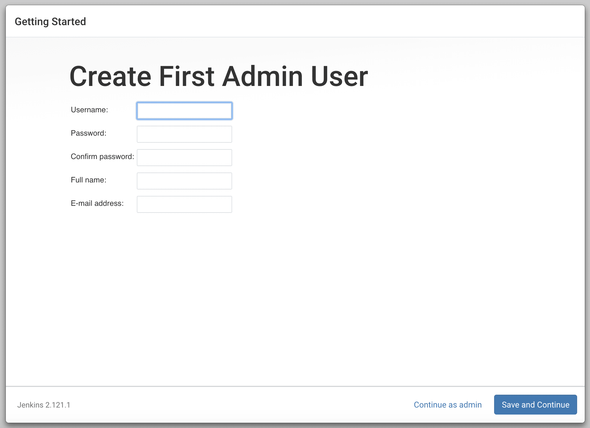
After installing all the basic plugins shown above, you will be redirected to another page for you to create your first admin user. This page is shown in the image below:

You can input all the admin user details and then click the `Save and Continue` button. You will then be redirected to another page as shown below:

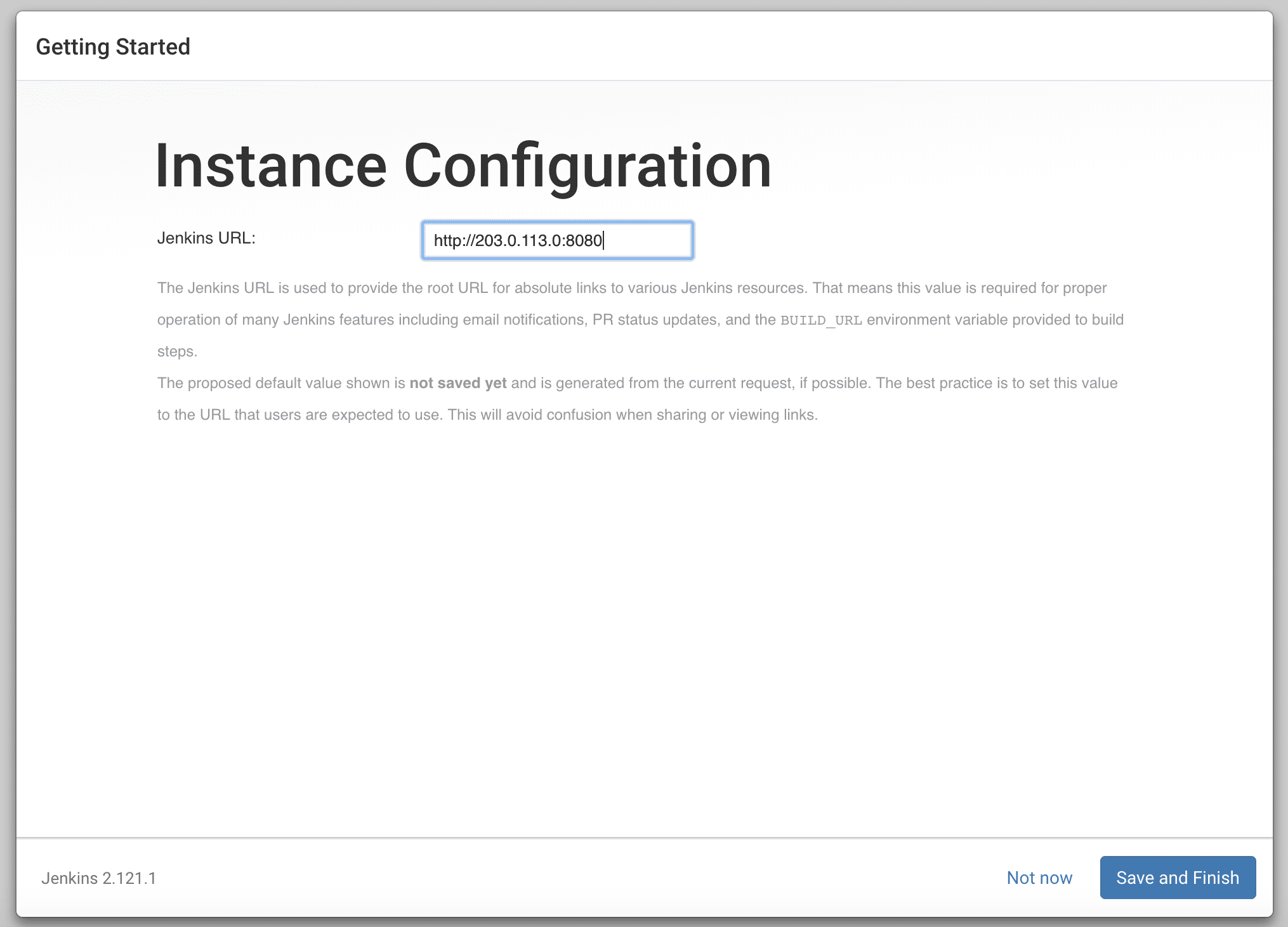
Adding Jenkins URL

You can add the Jenkins URL as shown below. This is the same URL http://127.0.0.1:8080 where Jenkins is running.

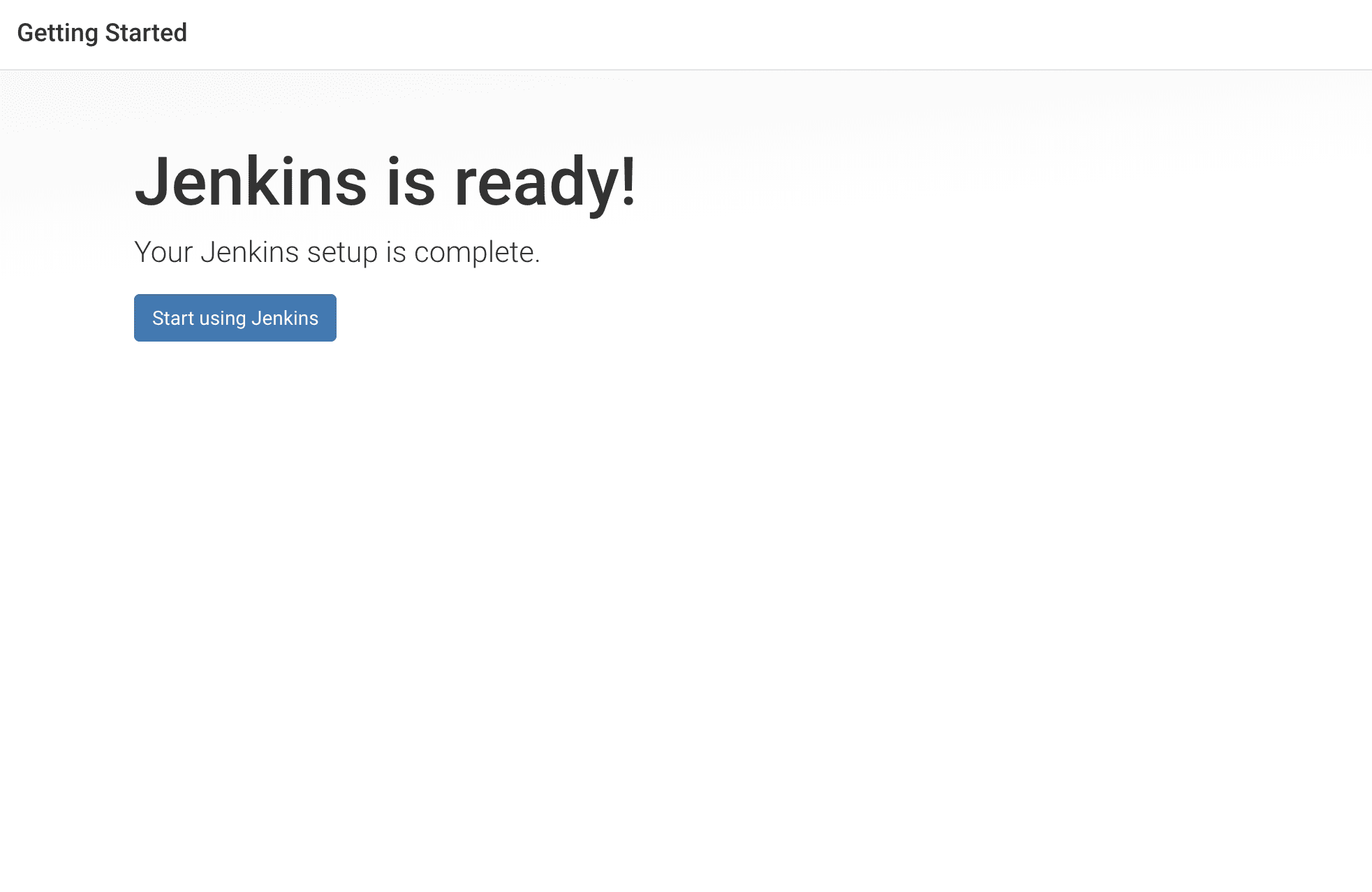
You can click `Save and Finish`. Your Jenkins platform will be running and ready to use. You will be redirected to another page as shown below:

Start using Jenkins

To start using Jenkins click on the `Start using Jenkins` button as shown in the image below:

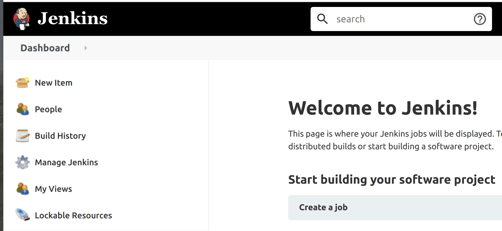
You can now start using Jenkins to create all your Jenkins CI/CD pipeline for automating the software development and deployment workflows. You will have access to the Jenkins Dashboard as shown below:

You have successfully set up Jenkins CI/CD on Kubernetes using Helm. You can access the Jenkins Dashboard.

Conclusion

In this tutorial, you have learned how to set up Jenkins CI/CD on Kubernetes Cluster using Helm. We used Helm because it’s one of the easiest ways of installing an application on the Kubernetes Cluster. This tutorial shows you how to install Helm on Linux, macOS, and Windows. It also shows you how to search for the Official Jenkins Helm Chart.

We also installed the official Jenkins Helm Chart on the Kubernetes Cluster using Helm.

Additionally, this tutorial shows you how to get your ‘admin’ password for unlocking Jenkins and how to login into Jenkins. In the end, we finished setting up Jenkins CI/CD on Kubernetes using Helm and accessed the Jenkins Dashboard. Hope this tutorial helps you in getting started with Jenkins.

The post How to Set up Jenkins CI/CD on Kubernetes Cluster using Helm appeared first on Simple Talk.


from Simple Talk https://ift.tt/KImj6sx
via

Thursday, September 14, 2023

The Pains and Joys of Making a Conference Schedule

Over the past 10 years, I have been involved in scheduling speakers at several conferences, most notably the PASS Data Community Summit. Since starting at Red-Gate last September, I have been much less involved in planning the Summit. Still, I have been able to help with the schedule by looking it over and looking for any inconsistencies, holes, or missing topics. Doing that reminded me of just how much of a pain it is, but also just how much joy there is when the schedule is released.

The first phase of making a schedule is choosing speakers. There is a delicate balance of skills, experience, topics, and even demographics that needs to be taken into account as you choose which speakers to call, and what topics you want presented. Good speakers get turned away every year from every conference because there are far more speakers than slots for them to speak.

The really challenging part comes once you have the set of speakers and sessions chosen: Making the schedule. The more days, the more slots, the more difficult. One of my previous colleagues I worked with on PASS Selection Committees, Jay Robinson, always referred to it as “Scheduling Sudoku”, which is an apt, if a bit basic description of the process. You have N number of rooms M number of slots, and you build out the schedule.

The difference between scheduling speakers and sudoku is in the latter you only need to consider the magnitude of each slot. Building a schedule requires you to consider a lot of complicated factors. For example:

  • Speaker requests: Speakers make requests all the time. This is something I never considered doing when I submit to speak. (With a few exceptions for expensive conferences), if I submit to speak, I generally plan to attend the entire conference even if I am not chosen.
  • Topic: Trying to spread out every topic over a conference gets more complicated than it sounds. You might have major topics (Databases versus UI coding), but then subtopics (Indexing, Query Tuning) that you also want to separate because they share a common underlying bond.
  • Speaker utilization: The big rule that can’t be broken sounds easy: “Don’t schedule a speaker against themselves.” Yet it happens. Sometimes they are a member of a panel that is not as obvious when you are doing the schedule. Sometimes they are expected to be in a non-speaking location. Sometimes it just is a mistake.
  • Demographics: You want to spread everyone out based on many characteristics, not the least of which is their employer. Also, don’t give anyone preferential treatment (which has many more meanings than you would expect).
  • Preferential treatment: Yep, even though I just said not to do this, there are regularly reasons that you have to put one speaker in a particular slot.
  • Overall mix of speakers to start and finish the conference: This was always hard. No one wants to be stuck in the final speaker slot (or day for that matter!). Everyone wants to be in the first slot so you can be done and go learn something. But organizers want people to have a reason to show up on that last day. Hence, you schedule a few great people on the final day and hope they forgive you. And that you don’t have to give them preferential treatment.

These are just the primary, even obvious, difficulties of making a schedule. What is exceptionally exciting is that all of these could change at any time. You can be 100% complete, reviewed, run up the flag pole, tested against all of your measuring sticks, and … you get the word that Speaker X has dropped out.

If you have ever actually played sudoku, you no doubt have reached that delightful stage of the game where you think you have solved it. Just a few more numbers to go. And then, there is one number that just won’t fit. Then you have to unravel your solution to get back to where everything does fit. Frustrating right? It is, but once you get all those darned numbers lined up, boy, is that a great feeling.

Today, the people who worked so diligently on the PASS Data Community Summit schedule get to see their fully filled out Schedule Sudoku entry and take a breath. Celebrate the victory. The schedule is done and ready for people to start planning their schedules. So hop over to passdatacommunitysummit.com/sessions/ and check out the schedule.


The post The Pains and Joys of Making a Conference Schedule appeared first on Simple Talk.


from Simple Talk https://ift.tt/jvuNkb8
via

Wednesday, September 13, 2023

Microsoft Fabric: Using notebooks and table partitioning to convert files to tables

When Microsoft Fabric was born, the only method to convert files to tables was using notebooks. Nowadays we have an easy-to-use UI feature for the conversion.

As I explained on the article about lakehouse and ETL, there are some scenarios where we still need to use notebooks for the conversion. One of these scenarios is when we need table partitioning.

Let’s make a step-by-step on this blog about how to use notebooks and table partitioning.

The steps explained here are based on the same sample data from the lakehouse and ETL article. In that article you can find the steps to build a pipeline to import the data to the files area.

The Starting Point

The starting point for this example is a lakehouse called demolake with the files already imported to the Files area using a pipeline.

No table is created yet.

Loading a Notebook

We will use a notebook for the conversion. You can download the notebook here. We will use the notebook called “01 – Create Delta Tables.ipynb”

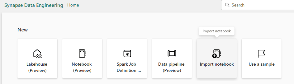
  1. Click the Experience button and select the Data Engineering Experience
  2. Click the Import Notebook button.

Interface gráfica do usuário, Aplicativo, Word Descrição gerada automaticamente

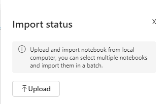
  1. Click the Upload button and select the notebook you just downloaded.

Interface gráfica do usuário, Texto, Aplicativo, Email Descrição gerada automaticamente

  1. Click the button lakehouse demo in the left button bar to return to the workspace.

Interface gráfica do usuário, Texto, Aplicativo Descrição gerada automaticamente

  1. Click on the notebook you imported.
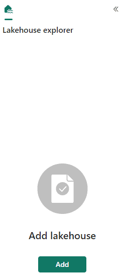
  2. On the Lakehouse explorer window, click the Add button to link the notebook to a lakehouse.

Interface gráfica do usuário, Aplicativo, Teams Descrição gerada automaticamente

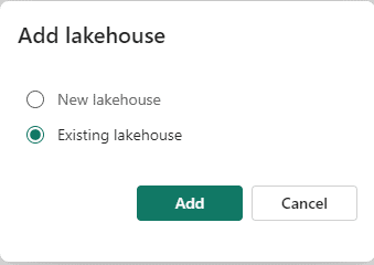
  1. On the Add Lakehouse window, select Existing Lakehouse and click the Add button.

Interface gráfica do usuário, Texto, Aplicativo, chat ou mensagem de texto Descrição gerada automaticamente

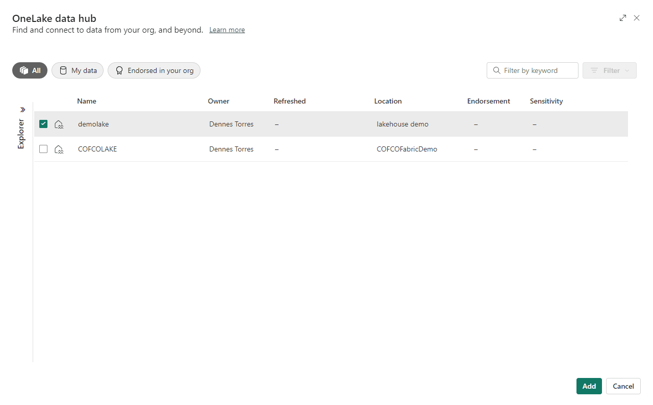
  1. Select the demolake and click the Add button.

Interface gráfica do usuário, Texto, Aplicativo, Email Descrição gerada automaticamente

The notebook code

Let’s analyse the code in the notebook we just imported.

First Code Block

# Copyright (c) Microsoft Corporation.
# Licensed under the MIT License.

spark.conf.set("sprk.sql.parquet.vorder.enabled", "true")

spark.conf.set("spark.microsoft.delta.optimizeWrite.enabled", "true")

spark.conf.set("spark.microsoft.delta.optimizeWrite.binSize", "1073741824")

This code block enables the V-Order optimization. This is a special optimization for delta tables. You can read more about the V-Order optimization on this link: https://learn.microsoft.com/en-us/fabric/data-engineering/delta-optimization-and-v-order?tabs=sparksql

The optimizeWrite option allow us to define what’s called binSize. This configuration defines the size for each parquet file used to store the data. Controlling the size of the files we can avoid too big files or too small files, either of these cases would cause a performance problem.

I would not be surprised if in the future some of these configurations may become a default.

Second Code Block

from pyspark.sql.functions import col, year, month, quarter

table_name = 'fact_sale'

df = spark.read.format("parquet").load('Files/fact_sale_1y_full')

df = df.withColumn('Year', year(col("InvoiceDateKey")))

df = df.withColumn('Quarter', quarter(col("InvoiceDateKey")))

df = df.withColumn('Month', month(col("InvoiceDateKey")))

df.write.mode("overwrite").format("delta").partitionBy("Year","Quarter").save("Tables/" + table_name)

This block executes the following tasks:

  • Read the fact_sale table from the Files folder.
  • Create a column called Year.
  • Create a column called Quarter.
  • Create a column called Month.
  • Save the data in the Tables area. The table is partitioned by Year and Quarter, and it will overwrite any existing table with the same name.

Third Code Block

from pyspark.sql.types import *
def loadFullDataFromSource(table_name):
    df = spark.read.format("parquet").load('Files/' + table_name)
    df.write.mode("overwrite").format("delta").save("Tables/" + table_name)

full_tables = [

'dimension_city',
'dimension_date',
'dimension_employee',
'dimension_stock_item'
 ]

for table in full_tables:
    loadFullDataFromSource(table)

This block has a function called loadFullDataFromSource. The function is defined in the beginning of the code, but it will only be executed when called.

The execution itself starts on the full_tables variable definition. This variable is an array with the name of the dimensions, which are also the name of the folders under the Files area in the lakehouse.

A FOR loop is executed over the table variable. For each dimension, the function loadFullDataFromSource is called receiving the name of the dimension as a parameter.

The function loads the data from the Files area and saves it to the Tables area using the table name as parameter. As a result, the function will load all the dimensions, one by one.

Executing the Notebook and checking the result

  1. Click the Run All button to execute all the code blocks in the notebook.

Microsoft Fabric uses a feature called Live Pool. We don’t need to configure a spark pool for the notebook execution. Every workspace linked with Fabric artifacts has the Live Pool enabled. Once we ask to execute a notebook or a single code block, the pool is enabled in very few seconds.

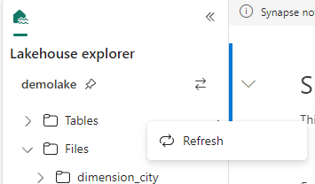
  1. On the lakehouse explorer, right click Tables and click Refresh.

Interface gráfica do usuário, Aplicativo Descrição gerada automaticamente

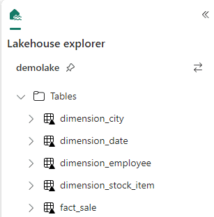
  1. The tables are now available in the Tables area.

Interface gráfica do usuário, Aplicativo Descrição gerada automaticamente

  1. On the left bar, click the demolake button.

Let’s look on the storage behind the tables in the lakehouse.

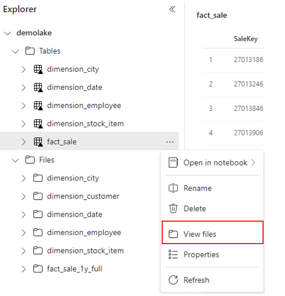
  1. Right click the fact_sale table
  2. On the context menu, click View files menu item.

Interface gráfica do usuário, Aplicativo Descrição gerada automaticamente

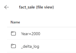
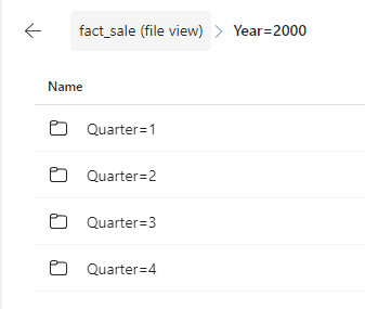
Mind how the files are stored in delta format and partitioned by Year and Quarter according to the configuration defined in the notebook.

Interface gráfica do usuário, Aplicativo Descrição gerada automaticamente

  1. Click the Year folder.

Interface gráfica do usuário, Aplicativo Descrição gerada automaticamente

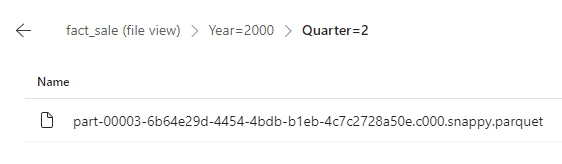
  1. Click one of the Quarters folder.

Interface gráfica do usuário, Texto, Aplicativo Descrição gerada automaticamente

Conclusion

On this blog you discovered how you can make the transformation from Files to Tables in a lakehouse using pyspark code and in this way be able to partition tables and schedule the code to make this movement.

The post Microsoft Fabric: Using notebooks and table partitioning to convert files to tables appeared first on Simple Talk.


from Simple Talk https://ift.tt/BM4Gzy6
via