The End of SQL Server 2008 and 2008 R2 Extended Support

If you are not already aware, SQL Server 2008 and SQL Server 2008 R2’s extended support will end on 9 July 2019. Microsoft has communicated this end date for a while now, including this announcement with resources on how to migrate from these two versions of Microsoft SQL Server.

What This Means

Microsoft has a defined lifecycle support policy, but there are two separate policies at the time of this article. The one SQL Server 2008 and SQL Server 2008 R2 fall into is known as the Fixed Lifecycle Policy. Under this policy, Microsoft commits to a minimum of 10 years of support, with at least five years of support each for Mainstream Support and Extended Support. What is the difference between the two? What happens when Extended Support ends?

Mainstream Support

Under Mainstream Support, customers get support both for incidents (issues with the application or system) and security updates. In addition, a customer can request product design and feature changes. If there is a bug found that isn’t security related, Microsoft may choose to fix it and release an update. Microsoft has rolled up many of these fixes into service packs and cumulative updates over the years.

Extended Support

Extended Support ends the regular incident support as well as requests for product design and feature changes unless a customer has a particular support contract now called Unified Support. Microsoft will continue to release security updates but will not typically release updates for other types of bugs. SQL Server 2008 and SQL Server 2008 R2 are in the fixed lifecycle until 9 July 2019.

Beyond Extended Support

Without being part of the Extended Support Update Program, there are no more updates, security or otherwise for your organisation once extended support ends. Only if Microsoft deems that a particular security vulnerability is sensitive enough will they decide to release a patch even for systems that are now in beyond extended support status. Microsoft has released patches a couple of times for out of support operating systems, but it should not be something you count on. I will talk more about Extended Support towards the end of this article when discussing what to do if you cannot migrate from SQL Server 2008 or SQL Server 2008 R2 in time.

Compliance Requirements

Depending on what industry standard, government regulations, and laws that apply to your organisation, you may be in a situation where you will be out of compliance should you have unsupported software. This would mean you would have to participate in the Extended Support Upgrade Program, incurring the expense of that program.

Reasons to Upgrade

If you are like me, you do not have a lot of spare time to upgrade a system for the sake of it. In IT there is always more to do than there is time to do it. Microsoft discontinuing support is a reasonable justification, but I would hope to get more out of an upgrade and the resulting chaos that always accompanies such efforts than just staying in support. The good news is that by upgrading from SQL Server 2008 or 2008 R2, there are additional features that you can put to immediate use. These features do not even require touching any applications. In addition, newer versions of SQL Server include plenty of features that would require some modification but are worth considering. Here is a list of some of this new functionality:

In Memory OLTP

Once upon a time, there was the DBCC PINTABLE() command, which allowed you to keep a table in memory for better performance. That stopped with SQL Server 2005, though the command was still present in that version of SQL Server. The idea was that SQL Server’s optimisation and fetch capabilities were robust enough to keep up with demand.

Of course, this did not hold true. As a result, Microsoft researched and developed Hekaton, which is an in-memory database option. Designed from the ground up, it doesn’t function at all like the old DBCC PINTABLE() command because how the data is stored is different. If you need the performance such an option provides, it became available with SQL Server 2014.

Columnstore Indexes

Most queries don’t require all the columns in a table. However, because a standard index is organised by row, you have to retrieve every row, and every column of every row, for each row which matches the query predicate. Conceptually, data is stored like this, with every column being kept together for a given row:

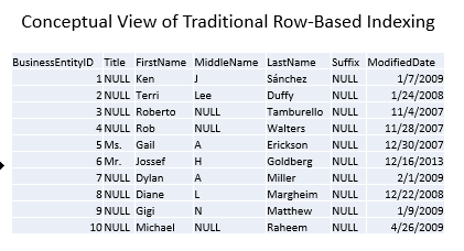
In other words, the engine is probably making a lot of extra reads to get the data you need. However, since that’s the way data is stored, you don’t have any other choice.

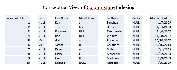
Columnstore indexes store the data in separate segments, one column per segment. A column can consist of more than one segment, but no segment can have more than one column. At a high level, you can think of the index working like this:

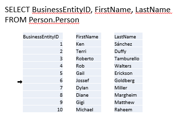
As a result, you just have to pull the segments related to the columns you care about, reading fewer pages and therefore achieving better performance. Continuing with the conceptual view, a query only wanting BusinessEntityID, FirstName, and LastName requires fewer reads because SQL Server doesn’t have to also grab data for Title, MiddleName, Suffix, and ModifiedDate simply to read in the entire row:

Columnstore Indexes are especially helpful in reporting and analytical scenarios with star or snowflake schema with a large fact table. The segmentation of the columns and the compression built into columnstore indexes means the query runs a lot faster than with a traditional index. However, this feature is not available until SQL Server 2012.

Availability Groups and Basic Availability Groups

If you have ever worked with traditional failover cluster instances, you understand the pains that this high availability (HA) option brings with it. The good news is that there is one instance, and all databases are highly available. The biggest bear of a requirement is the shared storage that all the nodes can access. This means you only have one set of the database files, and there is only one accessible copy of the data.

With a failover cluster instance, failover means stopping SQL Server on one node and starting it on another node. This can happen automatically, but during that failover, the SQL Server instance is unavailable.

With Availability Groups, introduced in SQL Server 2012, the HA is at the database level. Availability Groups do not require shared storage. In fact, Availability Groups do not use shared storage at all. This means you have more than one copy: at least one primary and from one to eight secondaries. These secondaries can be used for read-only access. In addition, there is technology that allows any of the partners (primary or secondary) to reach out to the other partners if a partner detects page-level corruption and get a correct page to replace the corrupted page. This feature is Automatic Page Repair.

Finally, with SQL Server 2016, Microsoft introduced Basic Availability Groups. Do you want the high availability but you do not need to access a secondary for read-only operations? Then you can take advantage of a basic availability group which only requires Standard Edition, therefore, it’s significantly cheaper.

Audit Object

One of the easiest ways to set up auditing is with the aptly named Audit object. However, when Microsoft first introduced this feature in SQL Server 2008, Microsoft deemed it was an Enterprise Edition only feature. While you can do similar things using Extended Events (actually, the Audit object is a set of Extended Events), it is not as easy to set up.

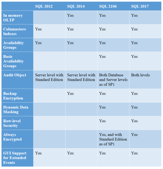
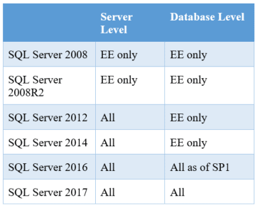
With industry’s need for auditing only growing, Microsoft has changed its stance in stages. Starting in SQL Server 2012, Microsoft enabled server-level auditing for Standard Edition. Then, in SQL Server 2016, starting with SP1, you can now use the Audit object at the database level with Standard Edition. Gaining access to Audit can be a huge benefit for compliance on our SQL Servers. I have found it helpful to have a quick chart:

Backup Encryption

When Microsoft introduced Transparent Data Encryption (TDE), it also introduced encrypted backups. However, initially, the encrypted backups were only for databases protected by TDE. TDE is an Enterprise Edition only feature. That meant you only had encrypted backups if you (a) were using Enterprise Edition and (b) had configured TDE on a particular database.

The third-party market (including Red Gate) has offered encryption in their SQL Server backup products for years. As a result, the community asked for Microsoft to also include backup encryption as a standard function for Microsoft SQL Server without having to use TDE. As a result, Microsoft added it to SQL Server 2014.

Backup encryption is crucial because smart attackers look for database backups. If an attacker can grab an unencrypted database backup, the attacker does not have to try and break into SQL Server. The attacker gets the same payoff but with less work. Therefore, if you can encrypt the database backups, especially if you belong to a firm without a third-party backup solution, you force the attackers to use a different, hopefully, more difficult method to get to the data. The more techniques an attacker must try, the more likely you are to discover the attempted hacking.

Dynamic Data Masking

I will admit to not being a fan of data masking. Solutions implementing data masking either leave the data at rest unmasked or they store the algorithm with the masked data in some form. This makes sense since privileged users must be able to see the real data. SQL Server is no different in this regard.

However, the purpose of SQL Server’s data masking is to provide a seamless solution for applications and users who shouldn’t see the actual data. You can define the masking algorithm. You can also define who can see the real data using a new permission, UNMASK. As long as you don’t change the data type/length of the field used in order to accommodate the masking algorithm, you can implement dynamic data masking without changing the application code or a user’s query unless they’re doing something to key off of the actual data.

Microsoft introduced this feature in SQL Server 2016, and its implementation can solve typical audit points around protecting the data in a system or report. As a result, it’s a great reason to upgrade from SQL Server 2008/2008R2 if you need to meet this sort of audit requirement.

Row-Level Security

You could implement row-level security solutions in SQL Server for years using views. However, there are some issues with this, as there are information disclosure issues with these home-grown solutions. The attack is basic: a savvy attacker can execute a query which reveals a bit about how the solution was built by forcing an error. A true, integrated row-level security solution was needed. As a result, Microsoft implemented row-level security as a feature first in Microsoft Azure and then in SQL Server 2016.

Speaking from experience, getting the home-grown solutions correct can be a problem. You have to be careful about how you write your filtering views or functions. Sometimes you’ll get duplicate rows because a security principal matches multiple ways for access. Therefore, you end up using the DISTINCT keyword or some similar method. Another issue is that often the security view or function is serialised, meaning performance is terrible in any system with more than a minimal load.

While you can still make mistakes on the performance side, you avoid the information disclosure issue and the row duplication issue.

Always Encrypted

When looking at encryption solutions for SQL Server, you should ask who can view the data. The focus is typically on the DBA or the administrator. Here are the three options:

1. DBAs can view the data.
2. DBAs cannot view the data but OS system administrators where SQL Server is installed can.
3. Neither the DBAs nor the system administrators can view the data.

System administrators are usually singled out for one of two reasons:

1. The DBAs also have administrative rights over the OS. In this case, #1 and #2 are the same level of permissions, meaning the DBAs can view the data.
2. The system administrators over the SQL Servers do not have permissions over the web or application servers.

If the DBAs can view the data, then you can use SQL Server’s built-in encryption mechanisms and let SQL Server perform key escrow using the standard pattern: database master key encrypts asymmetric key/certificate encrypts symmetric key encrypts data. If the DBAs cannot view the data and they aren’t system administrators but system administrators can (because they can see the system’s memory), then you can use the SQL Server built-in encryption, but you’ll need to have those keys encrypted by password, which the application has stored and uses. In either case, the built-in functions do the job, but they are hard to retrofit into an existing application, and they are not the easiest to use even if you are starting from scratch.

If neither the DBAs nor anyone who can access the system’s memory is allowed to view the data, then you cannot use SQL Server’s built-in encryption. The data must be encrypted before it reaches the SQL Server. Previously, this meant you had to build an encryption solution into the application. This is not typically a skillset for most developers. That means developers are operating out of their core body of knowledge, which means they work slower than they would like. It also means they may miss something important because they lack the knowledge to implement the encryption solution properly, despite their best efforts.

Another scenario is that you may need to retrofit an existing application to ensure that the data in the database in encrypted and/or the data in flight is encrypted. Retrofitting an application is expensive. The system is in production, so changes are the costliest at this point in the application’s lifecycle. Making these changes is going to require extensive testing just to maintain existing functionality. Wouldn’t it be great if the encryption/decryption could happen seamlessly to our application? That is what Always Encrypted does.

Always Encrypted is available starting with SQL Server 2016 (Enterprise Edition) or SQL Server 2016 SP1 (opened up for Standard Edition). Always Encrypted has a client on the application server. The client takes the database requests from the application and handles the encryption/decryption seamlessly. The back-end data in SQL Server is stored in a binary format, and while SQL Server has information on how the data is encrypted: the algorithm and metadata about the keys, however, the keys to decrypt are not stored with SQL Server. As a result, the DBA cannot decrypt the data unless the DBA has access to more than SQL Server or the OS where SQL Server is installed.

Better Support for Extended Events

Extended Events were introduced in SQL Server 2008, but they were not easy to use. For instance, there was no GUI to help set up and use Extended Events. The only way to work with Extended Events was via T-SQL.

Starting with SQL Server 2012, GUI support was introduced in SQL Server Management Studio (SSMS). With each new version of SQL Server, Microsoft extends what you can monitor with Extended Events (pun intended). The ability to capture information about new features is only instrumented with Extended Events. If you are still in “Camp Profiler,” you cannot monitor these features short of capturing every T-SQL statement or batch. That is not efficient.

One of the most important reasons to move off Profiler server-side traces and towards Extended Events is performance. The observer overhead for traces is generally higher than extended events, especially under CPU load. This is especially true using Profiler (the GUI) for monitoring SQL Server activity. Another area of performance improvement is with the filter/predicate. You can set a filter just like with Profiler. However, with Extended Events, the filtering is designed to happen as quickly as possible. SQL Server will honour the filter as it considers whether or not to capture an event. If it hits the filter, it cuts out and goes no further for that particular extended event set up. This is different than the deprecated trace behaviour. While trace will still apply the filter, it does so after the event/data collection has occurred, which results in “relatively little performance savings.” With these two improvements, Extended Events should capture only the data you specify, and it should cut out if it determines you aren’t actually interested in the event because of the filters you specified, meaning less load on the system due to monitoring.

That’s why, in the majority of cases, Extended Events are more lightweight than traditional traces. They certainly can capture more, especially if you are using any of the new features introduced from SQL Server 2012 and later. This, in and of itself, may be a great reason to migrate away from SQL Server 2008. After all, the better you can instrument your production environment while minimising the performance impact, the better.

Windowing Functions, DDL We’ve Cried For, and More, All in T-SQL

With every new version of SQL Server, Microsoft will add new features as well as improve existing ones. With SQL Server 2012, Microsoft introduced a significant amount of new functionality through T-SQL. Some of this functionality applied to queries, but others applied to configuration and database schema management. Here are three at three meaningful examples.

Windowing Functions

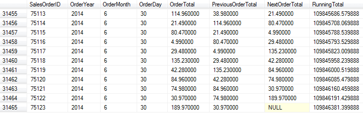
Window(ing) functions compute aggregations based on defined partitions. SQL Server 2008 and 2008R2 did have windowing functions using OVER() and PARTITION BY for ranking and aggregates. With SQL Server 2012 You get LAG() and LEAD(). You can also do more with aggregate functions. For instance, imagine the scenario where you had to report the order total for each order, but you also had to show the previous order total (LAG) and the next order total (LEAD). You might have another requirement, which is to show a running total. All of this can be put into a simple query:

SELECT SalesOrderID, OrderYear, OrderMonth, OrderDay, OrderTotal,
  LAG(OrderTotal, 1, 0) OVER (ORDER BY SalesOrderID) AS PreviousOrderTotal,
  LEAD(OrderTotal, 1) OVER (ORDER BY SalesOrderID) AS NextOrderTotal,
  SUM(OrderTotal) OVER (ORDER BY SalesOrderID ROWS BETWEEN UNBOUNDED PRECEDING 
                                              AND CURRENT ROW) AS RunningTotal
FROM
-- This subquery is to aggregate all the line items for an order
-- into a single total and simplify the year, month, day for
-- the query
(SELECT SOH.SalesOrderID, YEAR(SOH.OrderDate) AS 'OrderYear', 
  MONTH(SOH.OrderDate) AS 'OrderMonth', DAY(SOH.OrderDate) AS 'OrderDay', 
  SUM(SOD.LineTotal) AS OrderTotal
FROM Sales.SalesOrderDetail AS SOD
  JOIN Sales.SalesOrderHeader AS SOH
    ON SOD.SalesOrderID = SOH.SalesOrderID
GROUP BY SOH.SalesOrderID, SOH.OrderDate) SalesRawData;

The neatest function is SUM() because of the ORDER BY in the OVER() clause. Note that the query uses the keyword ROWS in the framing clause. This is new to SQL Server 2012, and the use of ROWS here tells SQL Server to add up all the rows prior to and including the current one. Since SQL Server is gathering the data at one time, the single query performs faster than having multiple queries trying to gather, re-gather, and calculate the same information. In addition, the data is all on the same row:

There are more window functions around rank distribution as well as the RANGE clause, which is similar in use to ROWS. SQL Server 2012 greatly expanded SQL Server’s window function support.

User-Defined Server Roles

When SQL Server 2005 debuted, it introduced a granular access model. A DBA could apply security to almost every object or feature of SQL Server. Microsoft pushed for the use of the new security model over the built-in database and server roles. However, at the time some server-level functionality keyed in on whether a login was in a role like sysadmin rather than checking to see if the login had the CONTROL permissions. As a result, DBAs stayed primarily with the roles that came with SQL Server.

The other issue was that SQL Server didn’t permit user-defined roles at the server level. Therefore, if a DBA wanted to implement a specific set of permissions at the server level using the granular model, that could be done, but it wasn’t tied to a role. This conflicted with the best practice of creating a role, assigning permissions to a role, and then granting membership to that role for the security principals (logins or users, in SQL Server’s case). DBAs could carry out this best practice at the database level, but not at the server level. With SQL Server 2012, server level user-defined roles are now possible. Therefore, it’s now possible to follow this best practice. However, you need to segment your permissions at the server level; you can create a role, assign the permissions, and then grant membership.

DROP IF EXISTS

A common problem DBAs face when handling deployments is when a script wants to create an object that already exists or the script wants to drop an object that isn’t there. To get around it, DBAs and developers have typically had to write code like this:

IF EXISTS(SELECT [name] FROM sys.objects WHERE name = ‘FooTable’)
  DROP TABLE FooTable;

Note that each of these statements must have the correct name. As a result, a DBA or developer putting together a deployment script updating hundreds of objects would need to verify each IF EXISTS() statement. Without third-party tools which do this sort of scripting for you, it can be cumbersome, especially in a large deployment. All that IF EXISTS() does is check for the existence of the object. Therefore, the community asked Microsoft for an IF EXISTS clause within the DROP statement that did the check and eliminated the need for this type of larger, more error-prone clause. Microsoft added this feature in SQL Server 2016. Now, you can simply do this:

DROP TABLE IF EXISTS FooTable;

If the table exists, SQL Server drops it. If the table doesn’t exist, SQL Server moves on without an error.

Ways to Migrate

Hopefully, you have gotten the go-ahead to migrate from your old SQL Server 2008/2008R2 instances to a new version. The next question is, “How?” One of the biggest concerns is breaking an existing application. There are some techniques to minimise these pains.

DNS is Your Friend

One of the chief concerns I hear about migrating database servers is, “I have to update all of my connections.” Sometimes this is followed by, “I’m not sure where all of them are, especially on the reporting side.” Here is where DNS can help.

I recommend trying to use “friendly” names in DNS that don’t refer to the server name, but to a generic name. Say there is an application called Brian’s Super Application. Rather than pointing to the actual server name of SQLServer144, you create an alias in DNS (a CNAME record in DNS parlance) called BriansSuperApp-SQL which is an alias to SQLSErver144. Then you can point the application to that friendlier name. If, at any point, the IP address on SQLServer144 changes, the CNAME will always be a reference to SQLServer144, meaning the client will get the correct IP address. Moreover, if you need to migrate to another SQL Server, say SQLServer278, simply change the alias. Point BriansSuperApp-SQL to SQLServer278, and the clients are repointed. You don’t have to change any connection information. This is an example of loose coupling applied to infrastructure.

But what if there are already applications configured to point directly to SQLServer144? Again, DNS can help. If you can migrate the databases and security from SQLServer144 to a newer SQL Server and then bring SQLServer144 off-line, you can use the same trick in DNS. Only instead of having a reference to BriansSuper-SQL that points to SQLServer278, you will delete all DNS records for SQLServer144 and then create a DNS record called SQLServer144 that points to SQLServer278. I have used this trick a lot in migrations, but it does require all the databases to move en masse to a single replacement server and the old server to be completely offline to work.

Remember Compatibility Levels

If your application requires a compatibility level of SQL Server 2008 or 2008R2, keep in mind that newer versions of SQL Server can support databases set to older versions of SQL Server via ALTER DATABASE. The compatibility designation for both SQL Server 2008 and 2008R2 is 100. All supported versions of SQL Server allow you to run a database in this compatibility mode. Therefore, you should be able to deploy to SQL Server 2017 (or 2019, if it is out by the time you are reading this).

Data Migration Assistant

What if you’re not sure if you can migrate from SQL Server 2008? Is there functionality that will break in the new version? Can you move the database to Azure? Trying to answer these questions can be a daunting task. However, Microsoft does have the Data Migration Assistant to assess your databases’ readiness to upgrade or move to Azure. Previously, DBAs would assess SQL Server Upgrade Advisor. Data Migration Assistant is extremely easy to use. First, you’ll need to create a project and tell DMA what you’re attempting to do:

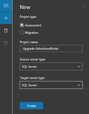
In this case, the assessment is for a SQL Server to SQL Server migration (on-premises). Then, you’ll need to tell DMA what to connect to and what to assess. Once DMA has verified it can connect and access the databases you’ve chosen, you’ll indicate what you what DMA to look at:

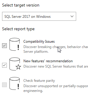
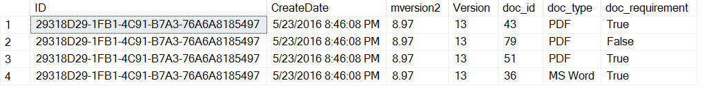
Here, the target specified is SQL Server 2017 and DMA is being instructed to not only look at compatibility issues but also to examine any new features that might be helpful. DMA will churn away and return its assessment:

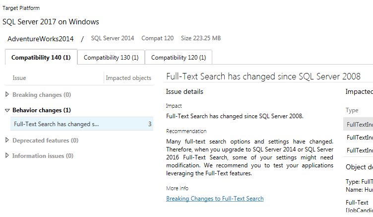
In this case, DMA noticed that Full-Text Search objects exist in the database. While DMA evaluated a SQL Server 2014 system and DB, note that DMA still flags a SQL Server 2008 issue. Like with any tool recommendations, you’ll need to consider whether the information presented applies in your case. Here, because DMA is looking at a SQL Server 2014 DB running on SQL Server 2014, there’s no issue with upgrading the database to a SQL Server 2017 instance.

Now AdventureWorks is a tiny, relatively simple database. You wouldn’t expect DMA to find much if anything. For your databases, especially large and complex ones, expect DMA to churn for a while and to have more recommendations and warnings.

What If You Can’t?

You may be in a situation where you cannot make a move by the deadline. What are your options? There are three:

Extended Security Updates

The first option, especially if you have to stay with on-premises SQL Servers, is to join the Extended Support Update program mentioned earlier. This is a pricy option, but it is the only way to maintain support for on-premises SQL Servers. Keep in mind, though, that in order to enroll in this program, Microsoft may very well ask for a migration plan on how and when you will move to supported versions of SQL Server.

Microsoft Azure

If you have the option of moving to a VM in Azure, then you will have additional coverage for three more years, as Microsoft indicated in a post on the Microsoft Azure blog. Microsoft has promised extended security updates at no extra cost if you are running on an Azure VM. In addition, the blog includes a reminder that a managed instance in Azure is another option for customers.

Again, you have to have the capability of moving to Azure. However, if you already in Azure or if you have been preparing to establish a presence, then an Azure VM may be a solution if you cannot migrate off SQL Server 2008 or 2008R2.

Go Without Support

The last option is to continue to run SQL Server 2008 or SQL Server 2008 R2 with no support. Your organisation may reason that Microsoft SQL Server has been relatively secure with only a handful of patches. There are a couple of issues, however.

The first issue is “you don’t know what you don’t know.” Someone may find a vulnerability tomorrow that is critical, easily exploitable, and which adversaries seize upon quickly. This was the case with SQL Slammer in the SQL Server 2000 days.

The second issue is around compliance. Some regulations, industry standards, and laws require systems to be running on supported, patched software. If your organisation is required to comply in such a manner, then going without support means the organisation is knowingly violating compliance and risks being caught. This is not just an immediate issue. After all, many regulations and laws can result in penalties and fines well after the period of non-compliance.

An organisation should only choose to go without support after a proper risk assessment. I know of cases where organisations decided to continue on NT 4 domains because they could not migrate to Active Directory. Other organisations have had key software that only ran on Windows 95, SQL Server 6.5, or some other ancient software. They could not find a proper replacement for that essential software and the business risk was more significant not to have the software or its functionality than running unsupported operating systems or software. However, those were informed decisions made after considering which was the greater risk.

Conclusion

With SQL Server 2008 and 2008 R2 extended support ending, it’s time to move off those database platforms. Even if you’re not required to upgrade from a GRC perspective, there’s a lot of functionality in the newer versions of SQL Server you can leverage for the benefit of your organisation. Microsoft has provided tools and guidance for upgrading. One example is the Data Migration Assistant. Microsoft has also provided additional documented guidance in SQL Docs to cover your migration scenario. If you can’t upgrade, but you require support, there are two paths you must choose from. The more costly option is to enter the Extended Support Upgrade program. The other path is to deploy to SQL Server 2008 instances in Microsoft Azure, as these will remain under support until 2022.

 

The post The End of SQL Server 2008 and 2008 R2 Extended Support appeared first on Simple Talk.

from Simple Talk http://bit.ly/2L9a60H
via

The State of SQL Server Monitoring 2019

Recently, over 800 participants across a range of sectors and from all around the globe took part in a survey about the state of SQL Server monitoring. This survey from Redgate Software is the only one of its kind and is in its second year. Here are some significant findings:

• Estates are continuing to grow
• Migrations are predicted to be the biggest challenge facing database professionals this year
• Adoption of cloud technologies is increasing
• Redgate’s SQL Server Monitor is the most popular third-party tool

The free report will be available on 25^th June. Be sure to join industry experts Grant Fritchey, Chris Yates, Annette Allen, and Tony Maddonna as they discuss key findings.

Monitoring SQL Server is critical for performance and security, and this report sheds light on the trends and challenges facing organisations in 2019.

 

The post The State of SQL Server Monitoring 2019 appeared first on Simple Talk.

from Simple Talk http://bit.ly/2YaV2TO
via

A MongoDB to SQL Server Migration: Data Typing and Un-nesting

When recently assigned a project to migrate data from MongoDB to SQL Server, my initial concern was my lack of expertise with MongoDB itself. I can say now after completing the project, MongoDB was the absolute least of my worries and certainly not a challenge. In fact, the ultimate solution that was implemented bypassed the MongoDB service altogether and used a combination of a MongoDB dump file and the native command line tool bsondump to convert the dump files from BSON (Binary JSON) to JSON for direct load into SQL Server tables. I was fortunate to avoid the C# coding required for that initial load step to pull the data into staging tables whose columns were all NVACHAR(MAX). (I have a very smart colleague, Lou Talarico, who noodled through that chore, and I have some references at the end of this article for further information). My tasks were simple comparatively: all I had to do was generate CREATE TABLE scripts with correct data types from the data in the staging tables and transpose the delimited array data stored in many of the columns. In this article, I will provide the sample data and code that will accomplish these two tasks.

The MongoDB Data

Most of us have had it drilled into our SQL brains for good reason that while NVARCHAR(MAX) has its place, it is not ideal for every column in every table. There is plenty of supporting evidence the you can find with a quick search that shows that the query optimizer does not always play nice when generating an optimal execution plan for these large data types. While it was the path of least resistance to use this data type to populate the SQL Server staging tables from the Extended JSON files MondoDB produced, it would not have been ideal for the final data types that the analysts would be writing queries against.

I decided to try and generate the code to create the final tables using a combination of metadata and a sampling of the actual data in staging tables. I would need to do this for each column and pull in any non-null values to determine what data type it should be including its max length. Before reviewing the code that will generate the final CREATE TABLE statements, take a look at some sample data so that you may understand the challenge.

Listing 1: Create and Populate Sample Table, doc_staging

CREATE TABLE [dbo].[doc_staging](
        [ID] [nvarchar](max) NULL,
        [CreateDate] [nvarchar](max) NULL,
        [mversion2] [nvarchar](max) NULL,
        [Version] [nvarchar](max) NULL,
        [doc_id] [nvarchar](max) NULL,
        [doc_type] [nvarchar](max) NULL,
        [doc_requirement] [nvarchar](max) NULL
) ON [PRIMARY] TEXTIMAGE_ON [PRIMARY]
GO
INSERT [dbo].[doc_staging] ([ID], [CreateDate], [mversion2], 
    [Version], [doc_id], [doc_type], [doc_requirement]) 
VALUES (N'7E3BB454-80B1-406D-9D8B-7223A412CEF8', N'4/10/2017 8:47:17 PM'
    , N'11.72', N'17', N'63||93||28||50||38', N'PDF||PDF||PDF||PDF||PDF'
    , N'True||True||True||True||True')
INSERT [dbo].[doc_staging] ([ID], [CreateDate], [mversion2],
    [Version], [doc_id], [doc_type], [doc_requirement]) 
VALUES (N'6BA95F5A-9A92-41AF-AD1E-588AEA39600C', N'3/11/2017 9:54:00 PM'
    , N'7.59', N'11', N'16||33||79||85||11', N'PDF||PDF||PDF||PDF||PDF' 
    , N'True||True||True||True||True')
INSERT [dbo].[doc_staging] ([ID], [CreateDate], [mversion2], 
    [Version], [doc_id], [doc_type], [doc_requirement]) 
VALUES (N'567FCEA7-F0E0-473B-94EA-127923FA0D36', N'3/14/2017 1:56:22 PM'
    , N'10.34', N'15', N'72||30||9||82||79||81||37'
    , N'PDF||PDF||PDF||PDF||PDF||PDF||PDF'
    , N'True||True||True||True||True||True||True')
INSERT [dbo].[doc_staging] ([ID], [CreateDate], [mversion2], 
    [Version], [doc_id], [doc_type], [doc_requirement]) 
VALUES (N'236FBDFD-857D-46E1-89EC-8A6911736145', N'3/4/2016 4:15:04 AM'
    , N'19.31', N'28', N'35||42||16||45||13||91||13'
    , N'PDF||PDF||PDF||PDF||PDF||PDF||MS Word'
    , N'True||True||True||True||True||True||True')
INSERT [dbo].[doc_staging] ([ID], [CreateDate], [mversion2], 
    [Version], [doc_id], [doc_type], [doc_requirement]) 
VALUES (N'EEBB9163-B88F-44F1-9F9F-ABEF0418EF78', N'3/31/2017 3:45:31 AM'
    , N'4.83', N'7', NULL, NULL, NULL)
INSERT [dbo].[doc_staging] ([ID], [CreateDate], [mversion2], 
    [Version], [doc_id], [doc_type], [doc_requirement]) 
VALUES (N'630644C3-6001-4B32-AF45-3C7EA6F0CA70', N'6/6/2016 1:30:11 AM'
    , N'5.52', N'8', N'63||18||92||54', N'PDF||PDF||PDF||PDF'
    , N'True||True||True||True')
INSERT [dbo].[doc_staging] ([ID], [CreateDate], [mversion2], 
    [Version], [doc_id], [doc_type], [doc_requirement]) 
VALUES (N'46998AA0-CCEA-41C5-9482-E94384FB11B0', N'8/11/2016 3:58:40 AM'
    , N'13.79', N'20', N'57', N'MS Word', N'True')
INSERT [dbo].[doc_staging] ([ID], [CreateDate], [mversion2], 
    [Version], [doc_id], [doc_type], [doc_requirement]) 
VALUES (N'695523CE-6DA4-4228-848C-3D92096AE18B', N'3/16/2017 3:27:06 PM'
    , N'13.10', N'19', N'95||22||12||81||86||94||67'
    , N'PDF||PDF||PDF||PDF||PDF||PDF||PDF'
    , N'True||True||True||True||True||True||True')
INSERT [dbo].[doc_staging] ([ID], [CreateDate], [mversion2], 
    [Version], [doc_id], [doc_type], [doc_requirement]) 
VALUES (N'C7802FCC-95D0-48D6-BC02-DE0704D64F45', N'5/12/2016 2:32:26 AM'
    , N'2.76', N'4', NULL, NULL, NULL)
INSERT [dbo].[doc_staging] ([ID], [CreateDate], [mversion2], 
    [Version], [doc_id], [doc_type], [doc_requirement]) 
VALUES (N'80D248F3-A6DC-440E-8845-3413E4ADDB88', N'5/24/2016 2:33:25 PM'
    , N'2.07', N'3', NULL, NULL, NULL)
INSERT [dbo].[doc_staging] ([ID], [CreateDate], [mversion2], 
    [Version], [doc_id], [doc_type], [doc_requirement]) 
VALUES (N'8FCE0A51-770B-43AF-997E-7B0D28236372', N'3/9/2017 9:57:52 PM'
    , N'11.72', N'17', N'98||90||89||2||97||50'
    , N'PDF||PDF||PDF||MS Word||MS Word||PDF'
    , N'True||True||True||False||True||True')
INSERT [dbo].[doc_staging] ([ID], [CreateDate], [mversion2], 
    [Version], [doc_id], [doc_type], [doc_requirement]) 
VALUES (N'29318D29-1FB1-4C91-B7A3-76A6A8185497', N'5/23/2016 8:46:08 PM'
    , N'8.97', N'13', N'43||79||51||36', N'PDF||PDF||PDF||MS Word'
    , N'True||True||True||True')

The above query creates the table and inserts 12 sample records. You can see that all of the columns use nvarchar(max) as the data type. The data itself contains common data types that will need to be converted, such as int, datetime and decimal.

Several fields are double pipe “||” delimited strings, each containing concatenated values. For example, doc_id in the first row has the value N’63||93||28||50||38′. In MongoDB, these were nested records in the collection, and this is how the conversion brought these over to the staging table, as one flat record. Further, the doc_id field is ordinally related to the doc_type and doc_requirements fields. The requirement is to transpose these values to individual rows for the final conversion. But first you have to build the ultimate, properly data typed “production” table.

The Solution

The following code builds the create table script and uses a simple iterative technique (thankfully not cursors) that reads each non-null value from each column, gleaned from the metadata in INFORMATION_SCHEMA.COLUMNS, and tries to ascertain the data type of the values. It is limited to a small set of data types like datetime, int, decimal and character-based values, but I have found it to be reliable and fast. Listing 2 shows the code in its entirety, commented to explain the process flow.

Listing 2: The code to create a CREATE TABLE script

SET nocount ON; 
--DECLARE variables and tables
DECLARE @Src NVARCHAR(max) 
DECLARE @Col NVARCHAR(max); 
DECLARE @SQL NVARCHAR(max); 
DECLARE @SQLCUR NVARCHAR(max); 
DECLARE @SQL_CASE NVARCHAR(max); 
DECLARE @maxlen INT; 
DECLARE @DB_Col TABLE 
  ( 
     rownum      INT, 
     column_name NVARCHAR(max) 
  ); 
DECLARE @Tablesrc NVARCHAR(max) 
DECLARE @MAX_Rec       INT, 
        @CURRENTRECORD INT; 
DECLARE @MAX_RecTAB       INT, 
        @CURRENTRECORDTAB INT; 
DECLARE @DT NVARCHAR(max) 
CREATE TABLE #temp 
  ( 
     #temp NVARCHAR(max) 
  ) 
CREATE TABLE #temp2 
  ( 
     #temp NVARCHAR(max) 
  ) 
--Create temp table #db_tab to hold table metadata 
--from INFORMATION_SCHEMA.TABLES
SELECT ROWNUM =Row_number() 
                 OVER ( 
                   ORDER BY table_name), 
       table_schema, 
       table_name 
INTO   #db_tab 
FROM   INFORMATION_SCHEMA.TABLES
--optional WHERE clause. If commented out, each user table in the 
--database will be returned
WHERE  table_name = 'doc_STAGING' 
--Set max record value for iteration through tables 
--(sample include only 1 table)
SET @CURRENTRECORDTAB = 1 
SET @MAX_RecTAB = (SELECT Max(rownum) 
                   FROM   #db_tab) 
--Iterate through each table                               
WHILE @CURRENTRECORDTAB <= @MAX_RecTAB 
  BEGIN 
      SELECT @Src = table_schema + '.' + table_name 
      FROM   #db_tab 
      WHERE  rownum = @CURRENTRECORDTAB 
--Remove "_staging" from the new table name
      SELECT @Tablesrc = Replace(table_name, '_STAGING', '') 
      FROM   #db_tab 
      WHERE  rownum = @CURRENTRECORDTAB 
--Populate next temp table variable "@DB_Col" with column metadata 
--from INFORMATION_SCHEMA.COLUMNS
      INSERT INTO @DB_Col 
      SELECT ROWNUM = Row_number() 
                        OVER ( 
                          ORDER BY ordinal_position), 
             column_name 
      FROM   INFORMATION_SCHEMA.COLUMNS 
      WHERE  table_schema + '.' + table_name = @Src
          
--Nested iteration for each column in the staging table
      SET @CURRENTRECORD = 1; 
--Begin building dynamic CREATE TABLE statement. DROP TABLE 
--can be optional
      --SET @SQL = N'DROP TABLE IF EXISTS ' + @Tablesrc + ';' 
      --           + Char(13) + Char(13) + '  CREATE TABLE dbo.' 
      --           + @Tablesrc + N' (' + Char(13); 
      SET @SQL =  '  CREATE TABLE dbo.' 
                 + @Tablesrc + N' (' + Char(13); 
--Get the max number of columns (ordinal_position field in 
--INFORMATION_SCHEMA.COLUMNS)
      SET @MAX_Rec = (SELECT Max(ordinal_position) 
                      FROM   INFORMATION_SCHEMA.COLUMNS 
                      WHERE  table_schema + '.' + table_name = @Src); 
--Start column iteration
      WHILE @CURRENTRECORD <= @MAX_Rec 
 --Set current column name using rownum
 BEGIN 
            SELECT @Col = N'[' + column_name + N']' 
            FROM   @DB_Col 
            WHERE  rownum = @CURRENTRECORD; 
--Get the max length of all non null values for current column
            SET @SQLCUR = N'Select   max(len(' + @Col + ')) from ' 
                + @Src + ' where ' + @Col + ' is not null'; 
            INSERT #temp 
            EXEC (@SQLCUR);
            SET @maxlen = (SELECT TOP 1 * 
                           FROM   #temp); 
--Round max length to nearest 10
            SET @maxlen = Round(@maxlen, -1); 
--This does all of the data type guessing work and writing the
-- output to a second temp table #temp2
           SET @SQL_CASE = N'Select TOP 1 CASE  WHEN Isdate(' + @Col 
                + N') = 1  AND ISNUMERIC(' + @Col 
                + N') <> 1 THEN ''DATETIME2'' WHEN ISNUMERIC(' + @Col 
                + N') = 1 and ' + @Col + N' 
                NOT LIKE ''%.%''THEN ''INT'' WHEN ISNUMERIC(' + @Col 
                + N') = 1 and ' + @Col 
                + N' LIKE ''%.%''THEN ''decimal(18,2)'' WHEN (isdate(' 
                + @Col + N') <> 1 and ISNUMERIC(' + @Col 
                + N') <> 1)  AND len(' + @Col + N') > 0 AND ' 
                + Cast(@maxlen AS VARCHAR(5)) 
                + ' < 4000 THEN ''NVARCHAR(' 
                + Cast(@maxlen + 20 AS VARCHAR(5)) 
                + N')'' ELSE ''NVARCHAR(MAX)'' END From ' 
                + @Src + ' where ' + @Col + N' is not null'; 
            INSERT #temp2 
            EXEC (@SQL_CASE); 
--Get the data type (@DT) from #temp2
            SET @DT = (SELECT TOP 1 * 
                       FROM   #temp2); 
            SET @SQL = @SQL + N'      ' + @Col + N' ' 
                       + Isnull(@DT, 'NVARCHAR(255)') + N',' + Char(13); 
  --We are finished with current column, let's delete these 
  --and get new ones
  DELETE FROM #temp;
  DELETE FROM #temp2; 
            SET @CURRENTRECORD = @CURRENTRECORD + 1; 
        END; 
--Build final SQL statement used to print CREATE TABLE 
--statement (optional EXEC)
      SET @SQL = LEFT(@SQL, ( Len(@SQL) - 2 )) 
      SET @SQl = @SQL + Char(13) + ')' 
 --Print the final CREATE TABLE SCRIPT
          PRINT @SQL; 
      SET @CURRENTRECORDTAB = @CURRENTRECORDTAB + 1; 
  END 
DROP TABLE [#db_tab];
DROP TABLE [#temp]; 
DROP TABLE [#temp2];

The code itself simply iterates through one or more tables, gathering metadata for column names and ordinal positions, interrogates each column to determine its max length and assumed data type and then generates a CREATE TABLE script, adding 20 to the rounded character-based fields. This version of the code uses Unicode data types. For the small sample table, it immediately returns the following:

CREATE TABLE dbo.doc (
      [ID] NVARCHAR(60),
      [CreateDate] DATETIME2,
      [mversion2] decimal(18,2),
      [Version] INT,
      [doc_id] NVARCHAR(80),
      [doc_type] NVARCHAR(140),
      [doc_requirement] NVARCHAR(110)
)

 

Notice that the _staging suffix has been removed and the final table will be dbo.doc. This, of course, is easily modifiable.

In the real project, there were tens of thousands of rows and the code still performed surprisingly well.

After running the CREATE TABLE statement to create the empty base table, appropriately data typed, it is time to populate it from the same staging data. Recall the requirement to transpose the delimited values from the doc_id, doc_type and doc_requirments columns so that these become a separate row.

You will need to transpose this:

43||79||51||36

Into this:

43

79

51

36

And further, you will need to join these doc_ids to their precise doc_type and doc_requirement values.

The figure below shows the first row, using the sample data.

The next figure shows what the final result should be. Notice that the doc_ids have maintained their ordinal positions despite their numerical order, which is crucial because the values in both doc_type and doc_requirement share the same positional location as the corresponding doc_id that they are related to.

Fortunately, there is a new function in SQL Server 2016 and higher called STRING_SPLIT() that handles this type of pivoting of delimited values with ease and does so very efficiently. The trick to getting these values to line up uses a combination of cross-applying the results of the STRING_SPLIT function with the base table and using the window function ROW_NUMBER to maintain the position.

The following listing shows the simple query to perform the work.

Listing 3: Splitting the field

SELECT *, arv.value AS doc_id_split, 
    Row_number() OVER (PARTITION BY id ORDER BY id ) AS RN 
FROM  [dbo].[doc_staging] 
CROSS apply String_split(Replace([doc_id], '||', '|'), N'|') arv

Notice that ROW_NUMBER is partitioned and ordered on the ID value of each row, which will return a running tally based on the number of delimited values that are cross applied.

You can then use the row number to join to the same cross applied row numbers for doc_type and doc_requirement. Remember each field to transpose has a variable number of actual delimited values; some rows may have five or more values, and others may only have one, but each row will contain the same number of doc_ids as there are doc_type and doc_requirement values.

It is also worth pointing out that the REPLACE function changes the double pipe to a single pipe character. Using the double pipe was a choice we made to have more assurance that there would not be actual data values that contain this combination of characters, but the downside is that the STRING_SPLIT function will only take a single byte value for the delimiter. Hence, the double pipe must be replaced with a single character delimiter. The final code to return exactly what is needed for the sample data, all 46 new rows, is in the following listing, which includes a CTE-based solution.

Listing 4: CTE to transpose the data values from the delimited values

WITH split_cte
AS (SELECT *,
           arv.value AS doc_id_split,
           ROW_NUMBER() OVER (PARTITION BY id ORDER BY id) AS RN
    FROM [dbo].[doc_staging]
        CROSS APPLY STRING_SPLIT(REPLACE([doc_id], '||', '|'), N'|') 
        arv),
     split_cte2
AS (SELECT id,
           arv2.value AS doc_type,
           ROW_NUMBER() OVER (PARTITION BY id ORDER BY id) AS RN
    FROM [dbo].[doc_staging]
        CROSS APPLY STRING_SPLIT(REPLACE([doc_type], '||', '|'), N'|') 
          arv2),
     split_cte3
AS (SELECT id,
           arv3.value AS doc_requirement,
           ROW_NUMBER() OVER (PARTITION BY id ORDER BY id) AS RN
    FROM [dbo].[doc_staging]
        CROSS APPLY STRING_SPLIT(REPLACE([doc_requirement], '||', '|')
           , N'|') arv3)
--INSERT INTO dbo.doc
SELECT sc1.ID,
       sc1.CreateDate,
       sc1.mversion2,
       sc1.Version,
       --,sc1.doc_id
       sc1.doc_id_split AS doc_id,
       sc2.doc_type,
       sc3.doc_requirement
FROM split_cte sc1
    INNER JOIN
    (SELECT id, split_cte2.doc_type, split_cte2.RN FROM split_cte2) sc2
        ON sc1.id = sc2.id
           AND sc1.RN = sc2.RN
    INNER JOIN
    (
        SELECT id,
               split_cte3.doc_requirement,
               split_cte3.RN
        FROM split_cte3
    ) sc3
        ON sc1.id = sc3.id
           AND sc1.RN = sc3.RN;

Each CTE splits one of the delimited columns, and the CTEs are joined together in the outer query. Since the OVER clause for ROW_NUMBER is identical in each case, they join together perfectly on the ID and row number.

By using this code, you can easily insert the results into the newly created dbo.doc table. I have commented out that insert statement so that you can see the results first.

Summary

I like the idea of having reusable code, even if it is to pick out certain pieces from a larger scope. I believe the code I am sharing here, which certainly has much room for improvement and extension, can be readily used for a variety of other purposes with some slight modification. One such goal would be to generate create table scripts for each table in an existing database. Instead of deriving the data type, it is possible just to use an existing data type. I will most likely go back to it many times for future projects that may involve a REST API, for example, rather than a MongoDB conversion. I know, too, that I will find a need to transpose delimited data somewhere down the road. Even if you do not have a specific need for a MongoDB conversion, I hope that the techniques shown here will help you in your projects.

References

For further information on the JSON framework used for the C# code as well as the bsondump utility, please see the following links.

https://www.newtonsoft.com/json

https://docs.mongodb.com/manual/reference/program/bsondump/

It is worth pointing out that the documentation for BSDUMP says that it is a diagnostic tool and not a tool for data ingestion or other application use.

 

The post A MongoDB to SQL Server Migration: Data Typing and Un-nesting appeared first on Simple Talk.

from Simple Talk http://bit.ly/2KueoR0
via

Keeping Kids Busy During Long School Breaks

Now that school is out for the summer, my grandson Thomas is spending quite a bit of time at our house. This year his parents decided that, at 12 years old, he was too old to go to a day-care/summer camp program. He will probably take over quite a bit of the yard work and participate in some other projects, but, otherwise, he will end up spending his free time playing video games.

To give him something educational to do, I bought a 3d printer. Neither of us had ever used one before, and it took us an afternoon to figure it out, especially since the instructions were not the best. For example, there were four different ways to attach the filament spool, and we managed to try the three wrong ways before getting it right. It was also tricky to detach the printed item once it was done. In both cases, Thomas figured out what to do. I was impressed with his troubleshooting and problem-solving skills.

To get started with a 3d printer, you can use premade files that are freely available on the web. This printer came with software that converts the file to the correct format (gcode) and saves it to an SD card. After inserting the SD card into the printer and following the commands on a little screen, you sit back and wait for the printer to do its job. It’s easy once you figure it out.

Now we are working on the next step: designing and creating our own objects. This is introducing him to computer-aided design software and getting him thinking more about geometry. (We are using TinkerCad.) I’m sure this will be highly educational and keep his brain busy, and he could even be developing skills for a future career.

The Raspberry Pi is another inexpensive yet educational piece of hardware. It was originally meant for teaching computer science to children but became so popular that it’s used for many useful projects, like creating a home VPN server or high-tech mirror that tells you the weather. I’m tempted to buy one of these for next summer, but finding the time to learn how to program it so I can teach him is a problem.

Even without buying a 3d printer or Raspberry Pi, there is no shortage of STEAM (science, technology, education, the arts, mathematics) projects that kids can do with things that you can find around the house. Visiting a science centre or makerspace for a day is another option, and many of these have camp programs.

Today’s children have grown up with technology like smartphones and tablets. It’s always been part of their lives. Showing them that they can do more, may or may not get them interested in learning how technology works. (I like driving my car, but I don’t want to build one!) I think it’s important that they all have the opportunity, however, because some of them will enjoy it, which could lead down a path to a great career.

Commentary Competition

Enjoyed the topic? Have a relevant anecdote? Disagree with the author? Leave your two cents on this post in the comments below, and our favourite response will win a $50 Amazon gift card. The competition closes two weeks from the date of publication, and the winner will be announced in the next Simple Talk newsletter.

The post Keeping Kids Busy During Long School Breaks appeared first on Simple Talk.

from Simple Talk http://bit.ly/2IsmU0E
via

Introduction to DevOps: The Evolving World of Application Delivery

The processes used to build and deploy today’s applications have undergone a dramatic shift. Efforts that were once segregated and performed in isolation are being joined into a single process flow that incorporates both development and operations. This new methodology, dubbed DevOps (a portmanteau of the two disciplines), bridges that gap between development and operations with the goal of delivering software more rapidly, frequently, and reliably.

This article is the first in a series about the DevOps movement and its impact on application building and delivery. In this series, I’ll introduce you to DevOps, provide an overview of the application delivery process, discuss issues that come with incorporating database management systems, and dig into specifics about security, privacy, and compliance. I’ll then tie up the series by discussing considerations to take into account when moving toward a DevOps model.

To help you get started, this article introduces you to DevOps and explains why this approach to application delivery is so important in today’s environment. As part of this discussion, I provide an overview of the advantages that DevOps offers and explain a few of the more important concepts that go into the DevOps process, with the proviso that I’ll be covering some of this information in more depth in subsequent articles.

Application Delivery Under Fire

Traditional approaches to application delivery place the development team on one side of the fence and IP operations on the other. The development team writes and tests the code, compiles it into neat little software packages, and tosses them over to the operations team, which deploys, integrates, and maintains the software, often in isolation from the other side.

This segregated approach to application delivery frequently relies on waterfall methodologies for building and deploying software. Waterfall development follows a logical progression of steps that start with gathering requirements and ends with application maintenance. The steps in between are carried out in a linear sequence, each with a distinct objective, such as defining the technical design, developing the code, or monitoring the application.

Figure 1 shows a representation of the waterfall methodology, in which the application delivery process is broken into five distinct steps—Plan, Develop, Test, Deploy, and Operate—with each step completed before the next one begins. In most cases, the tasks within a step are carried out by a single team (or individual), with relatively little cross-over between teams.

Figure 1. Traditional waterfall development

The steps shown in the figure are meant only to demonstrate the principles behind the waterfall methodology. In practice, the breakdown will likely be different and contain more steps. For example, the planning phase might be divided into two or more steps, such as gathering requirements, developing specifications, and designing the application. Regardless of the breakdown, the principles are the same: Each step is a discrete operation that is completed before moving on to the next step, similar to a cascading waterfall, or so the metaphor goes.

In the good ol’ days of simple desktop and client-server applications (accessed entirely behind the corporate firewall), the waterfall approach was usually more than adequate, providing a comprehensive, disciplined methodology with clearly defined roles and little room for deviation.

But we now live in an age of constant security threats, highly mobile users, and consumer-driven work models with little tolerance for disruption in services. In such an environment, application delivery processes based on a waterfall methodology or similar approaches are too inflexible, slow, and inefficient to meet today’s application challenges. And that’s where DevOps comes into the picture.

The Agile Connection

The DevOps story begins with the Agile approach to application delivery, which emphasises people and communication over processes and tools. Individuals work closely together to deliver software in quick and incremental cycles known as sprints. In each sprint, participants focus on a specific phase of the project, carrying out a small chunk of work in a defined period of time.

The Agile methodology has quickly supplanted the waterfall approach as the darling of development teams across organisations large and small. However, the model’s success also made it apparent that application delivery could achieve greater efficiency if development and operations worked more in concert with each other, rather than at odds—a realisation that has given rise to the DevOps movement.

DevOps attempts to bridge the gap between development and operations, which is something Agile doesn’t normally do. That said, the exact relationship between DevOps and Agile—or the differences between them—is not all that clearcut. Some people see DevOps as an extension of Agile, others see it as a replacement, and still others treat them as nearly one and the same. In fact, you’ll find a wide range of interpretations on how Agile and DevOps are related and how the two might differ.

But rather than add to this discussion here, I’ll say only that there seems to be at least some agreement that Agile and DevOps can serve as complementary approaches to application delivery, even if the lines between them are sometimes blurred.

A New Approach to Application Delivery

The DevOps approach calls for a shift in perspective from one that sees application delivery as a set of discrete, independent stages to one that incorporates the entire application delivery chain into a continuous, integrated process flow that includes everything from application design to system monitoring. The DevOps approach brings development and operations together with the goal of streamlining application building and deployment into an automated process that takes into account the entire delivery chain.

Under the DevOps model, application delivery is a continual workflow that essentially loops back onto itself to support a continuous process, as shown in Figure 2. You still have specific tasks that must be carried out, but they’re performed as an integrated whole that requires all participants to work together to keep the flow moving.

Figure 2. The DevOps process flow

As with the waterfall approach, DevOps can be represented in various ways. You’ll often see the process illustrated as a figure eight rather than as a circle or the tasks following a different outline. For example, the Develop stage might be broken into the Code and Build stages, the Deploy stage might be divided into the Release and Implement stages, and the Operate stage might be separated into the Operate and Monitor stages.

Regardless of how the DevOps process is illustrated, the important point is that application delivery is a unified, integrated process flow, rather than the type of linear, segregated phases you see in waterfall development. In a sense, transitioning from a waterfall to DevOps methodology is like moving from a two-dimensional line to a three-dimensional grid in which the intersection points are all connected.

DevOps and the CAMS model

At its core, DevOps is about creating a culture of collaboration and transparency that fosters open communications across all teams involved in application delivery. The DevOps approach seeks to break down siloes and encourage a sense of shared responsibility, creating an environment in which everyone works together to build and deploy software more effectively than with traditional methodologies.

Although discussions around DevOps often focus on coding and deploying the application, a successful DevOps effort also requires that quality assurance (QA), security and business considerations be fully integrated into the process flow, with support for the type of cross-team communications necessary to fully protect data and ensure the application’s success.

To this end, DevOps is often described in terms of the CAMS model (culture, automation, measurement and sharing). Together these four principles define the operational foundation on which DevOps is built:

• Culture: A transparent and collaborative environment that encourages communication and cooperation among participants, with processes and tools in place to support these efforts.
• Automation: The ongoing automation of repeatable and time-consuming tasks to create a unified workflow throughout the application delivery process.
• Measurement: The ability to monitor and track the various tasks performed throughout the application delivery process in order to correct and improve the DevOps workflow.
• Sharing: The ongoing sharing of knowledge, resources, and tools among all individuals participating in the DevOps workflow.

The four CAMS principles promise to make the application delivery process more efficient, flexible, and responsive to changing requirements. Because each cycle is shorter, application releases are available faster and more frequently.

With the DevOps approach, you don’t run into the types of knowledge transfer issues you get with traditional development efforts, which can lead to increased costs and risks. Team members own the entire lifecycle, sharing information and participating in the same processes while avoiding many of the communication breakdowns that afflict segregated teams. The DevOps approach also includes a built-in mechanism for constantly improving processes and streamlining operations, based on current requirements.

The DevOps Process Flow

To facilitate application delivery, the DevOps methodology leverages a number of tools and technologies that support the process flow. Together they create an automated application delivery pipeline that offers continuous integration, delivery, testing, deployment, and monitoring. Figure 3 updates the previous figure to reflect the integral role that the continuous services play in supporting the DevOps process flow.

Figure 3. The continuous services of the DevOps methodology

The continuous services streamline the application delivery process, making it possible to implement software faster and more efficiently:

• Continuous integration provides a mechanism for adding, updating, testing, and validating the code on a regular schedule.
• Continuous delivery works in conjunction with continuous integration to provide a structure for developing, testing, and deploying code as part of an integrated automated process.
• Continuous testing incorporates QA into the automated operations while supporting such tasks as unit and functional testing.
• Continuous deployment provides a structure for automatically releasing code that has been committed to the repository and has passed the automated testing phase.
• Continuous monitoring tracks and reports issues that occur during the application delivery process.

Several tools are available to help teams implement continuous DevOps services, including source control and configuration management solutions. A DevOps environment might also incorporate such technologies as containerization, microservices, or infrastructure as code. In the next tutorial, I’ll dig into the DevOps process flow in more detail to provide a better understanding of how all these pieces fit together.

Moving Toward the DevOps Model

Implementing the DevOps methodology requires personnel who have the ability to bridge development and operational boundaries, people who can speak both languages to bring application delivery under one roof.

Although the exact requirements will depend on an organisation’s size and type of development efforts, most organisations will require individuals with broader skillsets than those required for more traditional approaches to application delivery. For example, a DevOps team might want operation engineers that have some understanding of software development or developers who have experience with deployment processes and tools.

The DevOps methodology relies on having the right people and tools in place to carry out all phases of the application delivery process. That said, DevOps is more than just skills and tools. It’s a philosophy and culture that requires a different mindset from traditional approaches to application delivery. It’s about collaborating and communicating and bridging the gap between development and operations in a way that has not seemed possible or practical until now.

The post Introduction to DevOps: The Evolving World of Application Delivery appeared first on Simple Talk.

from Simple Talk https://www.red-gate.com/simple-talk/sysadmin/devops/introduction-to-devops-the-evolving-world-of-application-delivery/
via

How to Linux for SQL Server DBAs — Part 4

The series so far:

1. How to Linux for SQL Server DBAs — Part 1
2. How to Linux for SQL Server DBAs — Part 2
3. How to Linux for SQL Server DBAs — Part 3
4. How to Linux for SQL Server DBAs — Part 4

The series has covered a great breadth of technical concepts and, hopefully, you, the reader has had a chance to work along with the areas I’ve covered. I’ve attempted to create translations from database terms and concepts to the Operating System level, hoping to ease the transition to Linux for the SQL Server DBA. This shift is both a wish and a need. With the metamorphosis of Azure on Linux, along with DevOps fueling a single OS for ease of deployments, the day is coming when everything will run on Linux, with pods and containers housing whatever is needed, making it easier to lift and shift whenever required. As I’ve stressed in previous articles, the biggest hurdle for the Microsoft Data Platform specialist is that, unlike other database technologists, you’ll be less likely to have a Linux professional to refer to for assistance. Knowing how to perform tasks that commonly fell to those individuals will be pertinent to your future role in the industry.

In this article, I’m going to discuss advanced navigation and processes in Linux. Although moving from one directory tree to another within the command line is common, knowing how to execute a command to navigate a complex tree or locate something that isn’t in the current directory is essential to administration, just as walking is essential for a child to go from crawling to running.

Advanced Navigation

In the previous articles, I discussed how Linux interprets certain characters to signify where you are referring to in the directory tree.

.	Current directory
..	One directory up from the current location
./	Inside current directory
../	Inside one directory above the current one
~/.	Home directory from any location
pwd	Display current location path

You can also create environment variables to common, deep, and complex directory paths that you regularly use to lessen the amount of typing at the command line. This can be done as part of your profile, so it is set as soon as you log in or you can set it during your session. Your Linux admin may also set some aliases globally for any user that logs in, and some are set by the OS. The OS identifies them by the precursor symbol $. For the following example, my preferred method of listing files is to list them to include “all files, with listed permissions and information”. I don’t want to type out ls -la all the time and would prefer Linux to default to this whenever I use the ls command to list out files. This is a standard example of when you would use an alias and to create an alias at the session level I’d type in the following:

>alias ls=“ls -la”

If I would like to set this for my session every time I login, I can set this in my .bashrc, (bash remote command) file or secondary profile. The alias can be added, (without the $ prompt) to an empty line in either of those files and once executed either by logging in or executing, the alias is set for the session. As was discussed in earlier articles, this is similar to the environment variables and parameters in Windows and is specific to the unique user that is logged in at the time. When you switch from one user to another, you have the choice to set up the environment for the new user, too.

>. ~/.bashrc

The command above requests the following:

• post the prompt, (>) uses the “.” Signalling to execute the file immediately following the period.
• “~” is the symbol for the home directory of the current user, (which may be different than the original user that has logged in and then switched over to the current user).
• .bashrc is the remote command file which resides in the home directory for the current user.

Where environment variables are set or exported, depending on the Linux distribution, aliases don’t require any other command than “alias” the command or term you would like to use for your alias and then the command(s) and filters to execute when the alias is entered at the command line.

Take care not to use reserved words or an executable that is needed for something else. Consider the following poor choice in alias:

>alias sqlcmd=“ps -ef | grep sqlservr”

If I created the above, the sqlcmd command line utility to query the database would no longer refer to the executable.

Aliases can be set up in multiple ways, along with setting at the .bashrc or the .profile, aliases can also be set in a separate file to ease management for more complex environments, often named .bash_aliases. To view the aliases, (if any have been set for your current host and login) open your .bashrc file in your home directory and inspect them.

>cd .
>view .bashrc

To get out of the vi editor without saving, type :q! (colon q exclamation point).

>alias <alias name> = <full path to directory or executable needed for variable>

Environment Variables

Environment variables, may appear to be redundant after working with aliases, but they are much more robust and have more uses.

1. Variables, either set at the session or environment level can be used by sub processes using the getenv function, unlike aliases, which are only available to the parent.
2. Variables can be used anywhere in the command line, by simply calling them with the $ before the variable name, where an alias only works in an interactive mode.

An example of this would be:

>export ls_sql=“ps -ef | grep SQL”
>echo $ls_sql

This command would return all running SQL processes. While an alias:

>alias ls_sql=“ps -ef | grep SQL”
>echo ls_sql

The above would return ls_sql, as there isn’t a redirect that echo can retrieve. An example of a common environment variable would be similar to the following:

>export SQL_HOME = /opt/mssql/bin

To add it to the profile, change to the home directory and edit the .profile, (or add a .profile if you don’t already have one.) It’s a best practice to create a .profile file vs editing the host level .bash_rc file. This way, if you have more than one database or application environment that requires a unique configuration, you aren’t left with a set global file that must be updated each time.

>vi ~/.profile

Using the vi editor, proceed to the bottom line of the file and type o to go into INSERT mode. If environment variables are already listed, it’s a good idea to group them together and add headers and comments into the file to help ease the management of the file.

For this example, I’ve added three environment variables to ease managing my SQL database server:

• SQL_HOME for the bin directory, (SQL Executables)
• SQL_TOOLS for the shortcut to take me to sqlcmd
• SQL_DATA for my data directory

I’ve added the option to export the environment variables. It’s not always required, but exporting vs just setting the variable ensures that this is set at the session level, even after you’ve exited out. Note this profile executes the .bashrc beforehand and post the execution, sets the environment. If there are any conflicting settings in the previous file, it will be overwritten by this one, (previous SQL_HOME, etc.)

export SQL_HOME=/opt/mssql/bin
export SQL_TOOLS=/opt/mssql-tools/bin
export SQL_DATA=/var/opt/mssql/data

Once you add these three lines, save your changes and exit the .profile in vi by typing ESC :x (escape colon x). To execute this profile, just as you did with the alias and once logged in, run this:

>. .profile

If you are in another directory and need to run the .profile, you can make one simple change:

>. ~/.profile

You can now verify if your environment is properly set by echoing the environment variable(s). Each of the variables can be placed on the same line with the single echo statement, a space between each one and no commas required:

> echo $SQL_HOME $SQL_TOOLS $SQL_DATA

You can now use these environment variables for navigations and processing:

>cd $SQL_DATA
>ls

You no longer need to type in the full path to the data files but can use the variable to achieve the same thing. When you use these environment variables, the difference in keystrokes is quite evident. Without the environment parameter, you would need to type in the full path. This doesn’t just work for navigation, but also executables. Using the example of logging into the SQL database, instead of typing in the full path to the SQL Tools directory, you can instead substitute $SQL_TOOLS for the path to sqlcmd:

Echo $SQL_TOOLS
$SQL_TOOLS/sqlcmd -S localhost -U SA
use master;
GO
select count(*) from sysobjects;
go
exit

 

This eliminates more of the work that may seem tedious for those used to a GUI and contending with more command line than to what they’re accustomed.

Knowing What is What

As you begin to work with Linux, as I’ve noted previously, you will have Microsoft technologists that may be new to Linux. They won’t have the decades of experience with Unix environments that many database platforms were able to rely on. You should expect less mature host designs to be offered to you for your databases. With this, you may discover that some of the required libraries are missing or hosts are misconfigured.

When I first began with Unix, this was a common case. Many of the tools for administrators working with databases still hadn’t matured, so DBAs needed to know how to locate what was misconfigured, what was needed, and how to find what was what. The following utilities are incredibly valuable in solving those challenges. As with those missing libraries and modules, these utilities might be missing, so I will also include how to install each one of them.

>apt-get install findutils
>cd $SQL_HOME
>find sqlservr

Or, use a wildcard to locate it if you aren’t sure of the executable name:

>find sql*

This will search the current and all child tree directories for any file/directory/executable starting with sql. It’s case-sensitive, so ensure if you’re looking for SQL, you change how you perform your search.

As a Windows database administrator, you may have spent time reviewing the Windows environment path to discover that it was using the wrong version of installed software vs what your database required, (think ODBC driver, etc.). There is a similar utility that can assist you in Linux called WHICH. It will tell you which application is currently set to be used by the user and profile in the session where you’re working.

For this example, note in the process list that bash is showing in the list, but you forgot where it’s installed, (you are still new to Linux, so this is plausible…) By using the WHICH utility, you can find out it’s in the /bin directory:

>ps -ef
>which bash

If you are missing the which utility, you can install it by running the following commands, displayed for the two most popular flavors of Linux installation utilities.

>apt-get install system-tools
>yum install sysnet-tools

Processes

For each and every process that runs inside of the database on a Linux host, there is a separate program instruction, read or write on file on input from a system user behind it. Understanding how SQL Server on Linux is different than Windows is a critical first step in working with Linux processes.

As multi-threaded processing in Windows is normal for SQL Server, it’s also been ported over as part of the codebase that was migrated to Linux. This architecture is foreign to the Oracle DBA, where each foreground and background process has its own process in Linux, the SQL Server has two main processes with multi-threading underneath. find the value in the individual process power for the database administrator.

While SQL Server is multi-threaded, every allocation of memory is attached to a process in Linux. These threads are separated along clear boundaries in the application to ease the management between critical and non-critical processing for the application. There is still a significant difference between Windows services and Linux processes. Windows depends on a service, when started, to bring up multiple processes to an active state, making it fully functional. A process in Linux, on the other hand, can very often be stopped and restarted, with only a percentage of those processes critical to the overall application, allowing with silo’d management of application stacks.

This may critically change the way that SQL Server will run on Linux in the future. Consider the following challenge:

You’re experiencing a memory leak that is coming from SQL Server that performs the archiving of the transaction log. What if you could log into the Linux host and stop, (i.e. kill) only the process connected to the thread that writes data to the transaction log and have the rest of the database continue to operate as normal? For many database platforms, the process attached to the logging process would restart transparently, subsequently solving the issue. This is a benefit of having separate processes over multi-threaded as part of a service, as you see in the Windows operating system.

Just as you stop the SQL Server service on a Windows server, you can locate and “kill” the SQL Server main process on Linux to stop the SQL Server. This is similar to an “end task” command in the Task Manager, but you understand the implications. With many database platforms that have run on Linux/Unix for an extensive time, the DBA learns that there is a specific process that can be killed to force a shutdown, (as a last resort) such as with Oracle (where the PMON or SMON process will suffice) or with PostgreSQL.

With this type of process architecture in place, along with understanding the Linux kernel, which was covered in previous articles, it’s easier to understand why Linux servers rarely require a reboot. Processes are only loosely connected to the kernel and can be disconnected just as easy with a kill command. I’ve experienced only one time where a Linux host required a cycle because a kill would not suffice and it was due to an application issuing tens of thousands of processes to a single host, overwhelming the host, resulting in an inability to log into the host.

The Process Command

The process status utility is issued with the first letters of the two words (ps) and displays the running processes on the host where it’s executed. It’s native to both Linux and Unix, can be run from any directory from the command line and is essential for many when monitoring processes. It is a host-level executable and is available to any user who has privileges to the /usr/bin directory of applications that come standard with a Linux, (or Unix) server.

Similar utilities that provide information like PS are:

Lost	List of Files
Top	Lists resource usage and top processes
Strace	Trace that will include processes

From the command line, you can view processes with the PS command:

>ps

There are numerous arguments, but if you wished to print to screen all the active processes in a generic format, you could use the -A argument. In this example, note that now the SQL Server processes show up, where before, they were hidden as an application:

>ps -A

If you prefer the BSD format, you could use one of the following variations instead:

>ps au 
>ps axu

The most common argument combination for DBAs is the -ef, which is the full format argument. This format provides added information about resource usage. The format argument is case-sensitive, so you can use the full format, (-f) for the long list format, (-F).

>ps -ef
>ps -eF

It displays the most common information that’s important to DBAs:

• User ID
• Process ID
• Parent Process ID
• CPU Usage
• Start Time
• Time Running, (unless it has completed.)
• Command

It’s a clear view of what DBAs need 95% of the time, so they prefer this set of arguments more often than any other.

To display processes that are currently running, (not just active, but running) you can use the -x argument. The output will look very similar to the examples above, but it’s important to know the difference when you’re working on a heavily utilized host that requires more advanced arguments.

>ps -x

What if this were a very busy host and there was a significant amount of process running on it? Filtering is an essential part of cutting through the information returned to the screen, and that’s where the GREP utility comes in. If you wanted to query the processes and only return those with “sql” in the name, then the following command would return this:

>ps -ef | grep sql

You could also use this as part of logging by rerouting the output to a file instead of the screen:

>ps -ef | grep sql > /tmp/logfile.txt
>ls -la /tmp/logfile.txt

You can now view this file, and the output from the ps command will be present:

>view /tmp/logfile.txt

Note how the ps command has changed in the last line to the grep. This is because the grep that was the second utility executed after the ps is what was captured in the output.

As there may be a user that has switched over to another user, (covered in part III of this series of articles) you may want to see the original user that is running the command instead of who they are currently running the command as. You can do this with the -U argument. You must add the user, (name or user ID) that you wish to see if they are a switched user after the argument:

>ps -fU <username>

Using these commands grant you the first insight to shell scripting, something I’ll write about in future articles.

Process Monitoring

Process information can be used not just to identify what is running, but the resources that are used by any given process. This command can also be used as a diagnostic tool when behavior isn’t as expected.

Although SQL Server is still multi-threaded, requiring the user to go into the database to view allocation of resources, there is still value to understanding how to identify what processes are connected to the parent process on a Linux server for the SQL Server, both database and executable.

There are a few ways that this can be done and I’ll cover each one of them and why.

The first one sources from the correct installation by user and group of SQL Server. The recommendation is to create a MSSQL user and an MSINSTALL or MSDBA group. This provides an isolated and secure environment for a database installation on Linux. If this is done, it also provides a means of identifying what processes are connect to a running SQL Server.

You can search for all processes owned by the group name or group number. In the following example, you can inspect the processes owned by the MSINSTALL group:

>ps -fG MSINSTALL

If you use the current container installation you’ve been working with, the SQL Server is owned by root. This doesn’t stop you from identifying all processes owned by the database; it just requires you to perform an extra step.

First, identify the SQL parent ID:

>ps -ef | grep MSSQL

Use the parent ID, which is the Top ID before root that displayed in the tree of processes and use it to identify everything owned by it:

>ps -f --ppid <pid>

Before you begin to use the Process Status Utility as a diagnostic utility, there are important aspects of it to understand. You can print out a process tree that provides a more physical view of the process hierarchy.

>ps -e --forest

The output clearly displays the parent ID followed by each child in descending order. This can also be done for an individual process. You can do this for the SQL Server database like this:

>ps -ef --forest | grep -v grep |grep sqlservr

This command displays a very clean visual of how the processes are connected in SQL Server when running in Linux.

Conclusion

This article covered some more deep level investigation of how to set up an environment for easier support and use, along with advanced navigation. It also demonstrated how to dig into the process utility and how to find what processes are running and where. The next article in this series will take you on an introduction to BASH scripting. The Linux DBA can’t survive on Power Shell alone, and there are a lot of cool utilities built into Linux and available via BASH to empower you to do more with less in Linux.

The post How to Linux for SQL Server DBAs — Part 4 appeared first on Simple Talk.

from Simple Talk http://bit.ly/31D3MV8
via