Friday, February 28, 2020

Overview of Azure Cache for Redis

This article explains the Azure Cache for Redis and its features, the data types supported, and the pricing tiers available. It will demonstrate the steps to create an Azure Redis Cache from the Azure Portal. The article will also explain how to create a simple console app and connect this app with cache and exchange data.

Prerequisites

To follow along with this article, you will need:

  • Azure Account. You can create a free account here
  • Visual Studio 2017 and above. You can download it from here

What is Caching?

Caching is a mechanism to store frequently accessed data in a data store temporarily and retrieve this data for subsequent requests instead of extracting it from the original data source. This process improves the performance and availability of an application. Reading data from the database may be slower if it needs to execute complex queries.

Azure Cache for Redis

The Azure Redis Cache is a high-performance caching service that provides in-memory data store for faster retrieval of data. It is based on the open-source implementation Redis cache. This ensures low latency and high throughput by reducing the need to perform slow I/O operations. It also provides high availability, scalability, and security.

When a user uses an application, the application tries to read data from the cache. If the requested data not available in the cache, the application gets the data from the actual data source. Then the application stores that data in the cache for subsequent requests. When the next request comes to an application, it retrieves data from the cache without going to the actual data source. This process improves the application performance because data lives in memory. Also, it increases the availability of an application in case of unavailability of the database. Figure 1 shows the cache workflow.

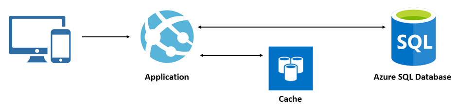
Figure 1: Cache Workflow

Features

Azure Cache for Redis has many features for management, performance, and high availability. Here are a few of the most important:

Fully Managed Service

Azure Redis Cache is a fully managed version of an open-source Redis server. i.e., it monitors, manages, hosting, and secure the service by default.

High Performance

Azure Redis cache enables an application to be responsive even the user load increases. It does so by leveraging the low latency, high-throughput capabilities of the Redis engine.

Geo-replication

Azure Redis cache allows replicating or syncing the cache in multiple regions in the world. One cache is primary, and other caches act as secondaries. The primary cache has read and write capabilities, but the secondary caches are read-only. If the primary goes down, then one secondary cache becomes primary. The significant advantage of this is high availability and reliability.

Cache Cluster

The cluster automatically shards the data in the cache across multiple Azure Cache for Redis nodes. A cluster increases performance and availability. Each shard node is made of two instances. When one instance goes down, the application still works because other instances in the cluster are running.

Data Persistence

Azure Redis cache persists the data by taking snapshots and backing up the data.

Data Types

Azure Redis Cache supports to store data in various formats. It supports data structures like Strings, Lists, Sets, and Hashes.

  • Strings: Redis strings are binary safe and allow them to store any type of data with serialization. The maximum allowed string length is 512MB. It provides some useful commands like Incr, Desr, Append, GetRange, SetRange, and other useful commands.
  • Lists: Lists are lists of Strings, sorted by insertion order. It allows adding elements at the beginning or end of the list. It supports constant time insertion and deletion of elements near the beginning or end of the list, even with many millions of inserted items.
  • Sets: These are also lists of Strings. The unique feature of sets is that they don’t allow duplicate values. There are two types of sets: Ordered and Unordered Sets.
  • Hashes: Hashes are objects, contains multiple fields. The object allows storing as many fields as required.

Pricing Tiers

Azure Redis Cache has three pricing layers with different features, performance, and budget.

  • Basic: Basic cache is a single node cache which is ideal for development/test and non-critical workloads. There’s no SLA (Service Level Agreement is Microsoft’s commitments for uptime and connectivity). The basic tier has different options to choose from C0 to C6. The lowest option is C0, and this is in a shared infrastructure. Everything above C0 provides dedicated service, i.e., this does not share infrastructure with other customers.
  • Standard: This tier offers an SLA and provides a replicated cache. The data is automatically replicated between the two nodes — ideal for production-level applications.
  • Premium: The Premium tier has all the standard features and, also, it provides better performance, bigger workloads, enhanced security, and disaster recovery. Backups and Snapshots and can be created and restored in case of failures. It also offers Redis Persistence, which persists data stored inside the cache. It also provides a Redis Cluster, which automatically shares data across multiple Redis nodes. Hence this allows creating workloads of bigger memory sizes and get better performance. It also offers support for Azure Virtual Networks, which gives the ability to isolate the cache by using subnets, access control policies, and other features.

Cache Invalidation

Cache Invalidation is the process of replacing or removing the cached items. If the data in the cache is deleted or invalid, then the application gets the latest data from the database and keeps it in the cache, and subsequent requests get the latest data from the cache.

There are different ways to invalidate the cache.

  • An application can remove the data in the cache
  • Configure the invalidation rule while setting up the cache
    • Set absolute expiration – you can set a specific time period to expire the cache
    • Set sliding expiration – If the data in the cache not touched for a certain amount of time, then delete the cache

Create an Azure Cache for Redis

Sign in to the Azure portal, click on the portal menu and select Create a resource menu option as shown in Figure 2.

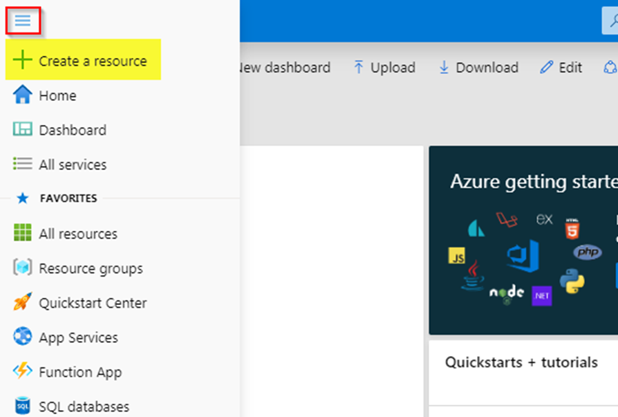
Figure 2: Microsoft Azure Portal Menu

In the next screen, Figure 3, type Azure Cache for Redis in the search bar and hit enter. This navigates to the Azure Cache for Redis window.

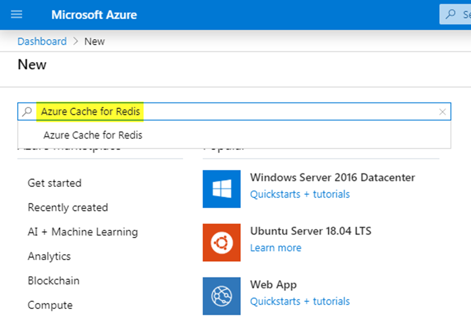
Figure 3: Microsoft Azure Marketplace

In the next screen, Figure 4, Azure Cache for Redis window, click on the Create button.

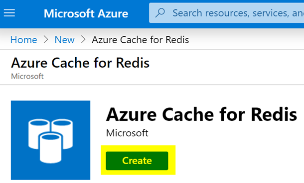
Figure 4: Azure Cache for Redis window

In the next screen, Figure 5, New Redis Cache window, fill out the unique DNS name, Subscription, Resource group, Location, Pricing tier, and all required information.

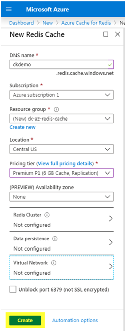
Figure 5: New Redis Cache window

Click View full pricing details. It opens a window (Figure 6) with available pricing tiers. Choosing the pricing tier is essential because this determines the performance of the cache, budget, and other features like dedicated or shared cache infrastructure, SLA, Redis cluster, data persistence, and data import and export.

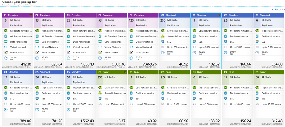
Figure 6: Pricing tier options

If you choose one of the Premium tiers, you can configure the cluster by clicking Redis Cluster (Figure 7). You can enable or disable clustering and select the shard count. Note that each shard is comprised of two instances.

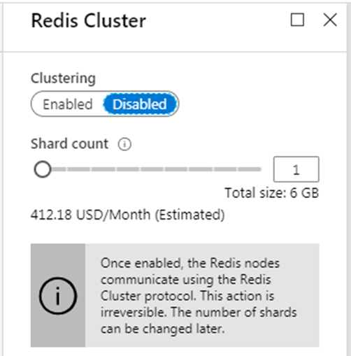
Figure 7: Redis Cluster Configuration

Data Persistence also requires the Premium tier. Figure 8 shows the configuration to persist the data stored in the cache. There are a couple of options to persist the data.

RDB (Redis database) persistence: This option persists the data by taking a snapshot of the cache. The snapshot is taken based on the frequency configured. In the case of recovery, the most recent snapshot will be used.

AOF (Append only file) persistence: This option saves the data for every writes operation. In case of recovery, the cache is reconstruct using stored write operation.

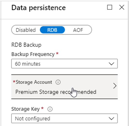
Figure 8: Data Persistence configuration

After filling out the required fields on the New Redis Cache window, click on the Create button. After a few minutes, the Azure Redis cache created and running.

Figure 9 shows the Azure Cache for Redis Overview. By default, it is secure because the Non-SSL port is disabled.

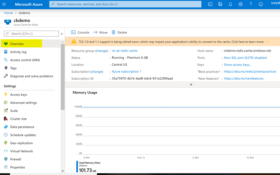
Figure 9: Overview of Azure Redis Cache

Create a Console App to Use the Cache

To try out the cache, you will create a Console app. Begin by opening Visual Studio and selecting File New Project.

The next screen, Figure 10, is the New Project window. Select the Console App (.Net Framework), fill out the project name and location, and click on the OK button.

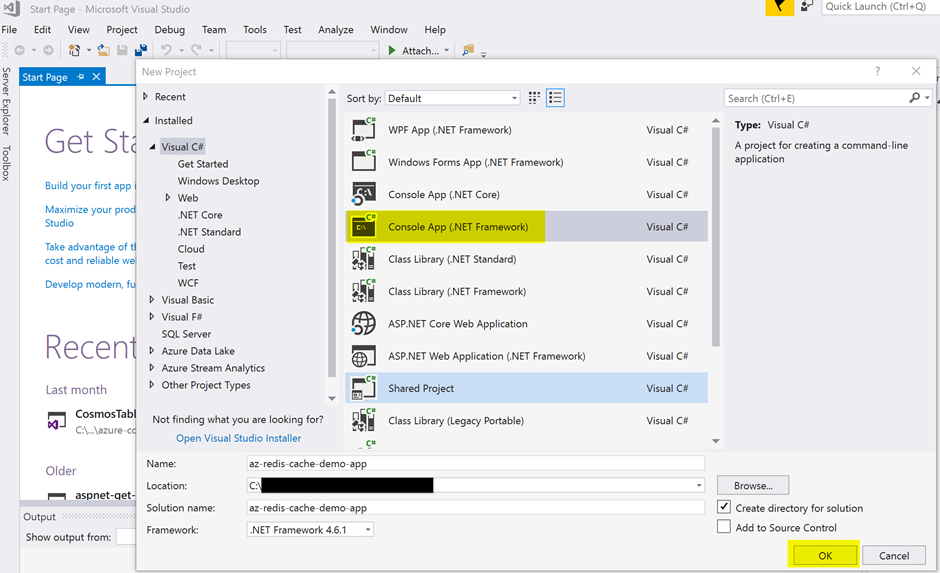
Figure 10: Visual Studio New Project

The next screen, Figure 11, shows the new console app.

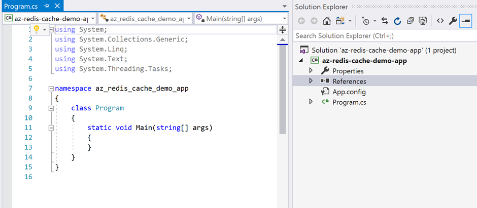
Figure 11: Visual Studio Console App

To connect the Console App to the Azure Redis Cache, you need to install Microsoft.Extensions.Caching.Redis package. To install this package from Visual Studio, go to Tools NuGet Package Manager Manage NuGet Packages for solution…

Figure 12 is the NuGet Package Manager. Make sure that Browse is selected. In the search bar type Microsoft.Extensions.Caching.Redis and select the package from the displayed list. Scroll down and click on the Install button.

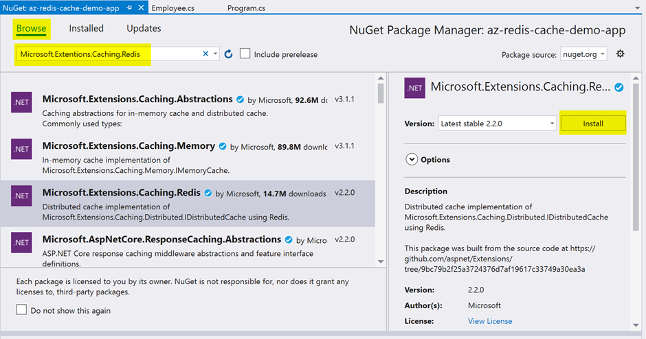
Figure 12: NuGet Package Manager

In the next screen, Figure 13, install Newtonsoft.Json package for serialization and deserialization of objects.

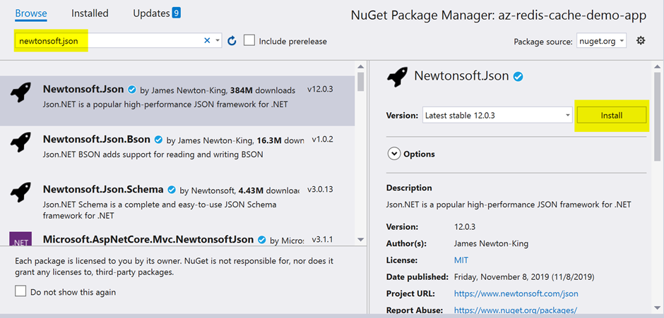
Figure 13: Install Newtonsoft.Json package

The console app can be connected to the Azure Redis Cache programmatically by using the Access keys of the Azure Redis Cache created in the Azure portal. In the next screen, Figure 14, go to the Azure Portal Redis Cache and click on the Access Keys tab and copy the Primary connection string.

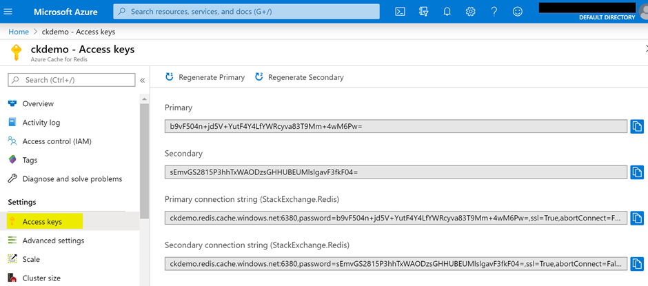
Figure 14: Access Keys from Azure Portal

Figure 15 shows the code after adding Redis cache connection string that you copied from the Azure portal to App.config file in the console app.

<appSettings>
    <add key="CacheConnection"
         value="<YOUR CONNECTION STRING>"/>
</appSettings>

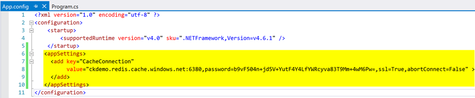
Figure 15: Configure Redis cache connection string in app.config

In real-world scenario applications, this connection string or credentials should be stored and accessed more securely.

In the next screen, Figure 16, get the Redis connection string defined in the app.config file in the program.cs file by using the ConfiguationManager class. Add the code to the Program class. The ConnectionMultiplexer class manages the connection with Azure Redis cache. Be sure to include references to System.Configuration and StackExchange.Redis.

private static Lazy<ConnectionMultiplexer> redisConnection = 
           new Lazy<ConnectionMultiplexer>(() =>
            {
                string cacheConnection = 
            ConfigurationManager.AppSettings["CacheConnection"].ToString();
                return ConnectionMultiplexer.Connect(cacheConnection);
            });
        public static ConnectionMultiplexer Connection
        {
            get
            {
                return redisConnection.Value;
            }
        }

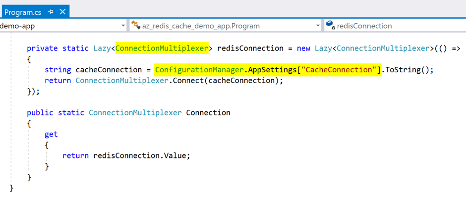
Figure 16: Managing Redis cache connection


Create a class called Employee; this acts as the data source for the console app.

The code for program.cs can be found below. First, the application gets the reference for the Redis cache database. Using that reference, the app checks whether data available in the cache. If it is available, read the data from the cache; otherwise, read the data from the actual data source and save it into the Azure Redis cache. For subsequent calls, data read from the cache.

using System;
using System.Collections.Generic;
using System.Configuration;
using StackExchange.Redis;
using Newtonsoft.Json;
namespace az_redis_cache_demo_app
{
    class Program
    {
        static void Main(string[] args)
        {
            Console.WriteLine("Azure Redis Cache Demo");
            Console.WriteLine("----------------------");
            Employee clsEmp = new Employee();
            List<Employee> lstEmployees = new List<Employee>();
            //Get the redis cache reference 
            IDatabase cache = redisConnection.Value.GetDatabase();
            //Get employee data from cache
            Console.WriteLine("Get employee data from Cache");
            var cachedEmployees = cache.StringGet("employees");
            //Check whether cache contains employee data
            if(string.IsNullOrEmpty(cachedEmployees))
            {
                //Cache doesn't have employee data and gets the 
                //data from actual data source
                Console.WriteLine("Employee data not available in the 
                   cache. Get data from actual data source");
                lstEmployees = clsEmp.GetEmployees();
                //After getting the employee data from the actual data 
                //source, Save that data in cache 
                Console.WriteLine("Set the employee data to Cache");
                cache.StringSet("employees", 
                JsonConvert.SerializeObject(lstEmployees));
            }
            else
            {
                //Cache contains employee data and deserializes the data
                Console.WriteLine("Employee data available in the 
                     cache. Read data from the Cache");
                lstEmployees = 
                    JsonConvert.DeserializeObject<List<Employee>>(
                          cachedEmployees);
            }
            
            //Print the employee data to console
            foreach (var emp in lstEmployees)
            {
                Console.WriteLine(emp.FirstName + " " + emp.LastName 
                            + ", " +       
                 emp.EmployeeId + ", " + emp.Salary + ", " 
                            + emp.Address);
            }
            Console.ReadLine();
        }
        private static Lazy<ConnectionMultiplexer> redisConnection 
                = new Lazy<ConnectionMultiplexer>(() =>
        {
            string cacheConnection = 
            ConfigurationManager.AppSettings["CacheConnection"].ToString();
            return ConnectionMultiplexer.Connect(cacheConnection);
        });
        public static ConnectionMultiplexer Connection
        {
            get
            {
                return redisConnection.Value;
            }
        }
    }
}

Figure 17 shows the code for the new Employee class.

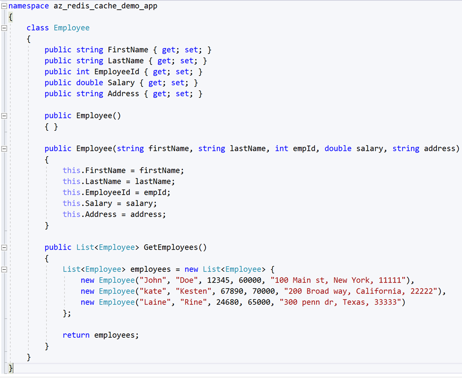
Figure 17: Employee class in the Console App

Run the application. The first time, data is not available in Redis cache, and the app gets data from the data source. See below Figure 18 for the console output.

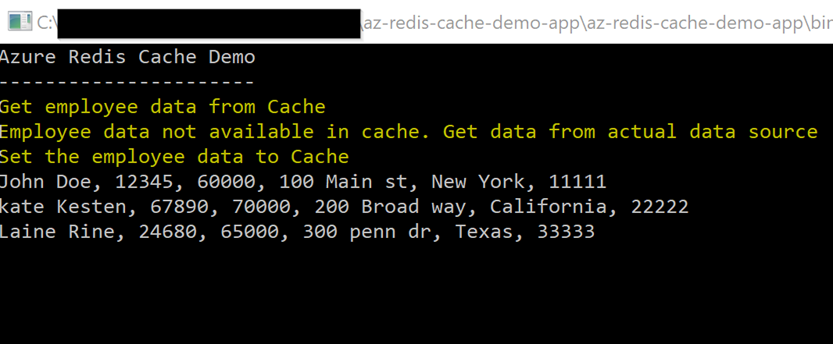
Figure 18: Console output window – first time run the application

In the next screen, Figure 19, is the result of subsequent calls. The application read the data from the Redis cache.

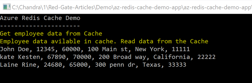
Figure 19: Console output window – Subsequent calls

You can also see the activity in the Azure Portal. Navigate to your Azure Cache for Redis and click Metrics. There you can filter the activity. In Figure 20, the metrics show that data is writing to the cache.

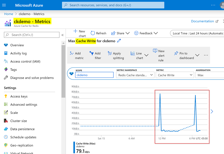
Figure 20: Redis cache write metrics from the Azure portal

In the next screen, Figure 21, Azure portal Redis cache metrics confirm that data is reading from the cache.

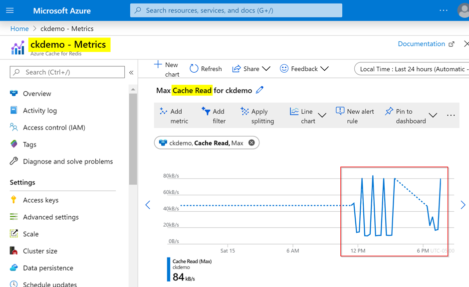
Figure 21: Redis cache read metrics from the Azure portal

Conclusion

This article explained the Azure Cache for Redis basics and demonstrated how to provision the Redis cache in the Azure Portal. It then showed how to connect it with a console app and read the data from the cache. In this way, Azure Cache for Redis allows reading data from the cache without going to the actual data source.

Reference Links

  • Click here for Azure Cache for Redis documentation
  • Click here for Redis open source documentation
  • Click here for Azure cache features, pricing and azure portal login

The post Overview of Azure Cache for Redis appeared first on Simple Talk.


from Simple Talk https://ift.tt/397H1Ma
via

Thursday, February 27, 2020

Mixing Relational and Graph DB Objects (Book and Session Prep)

Graph structures are something that I have lightly covered in my Database Design book in the last few book editions (the last coinciding with SQL Server 2016), implementing them with relational tables. In the next edition of my book that I am starting to write now, my goal will be to cover one of the most important new topics for database design in SQL Server: using the graph db extensions added in SQL Server 2017.

Before SQL Server 2017, the techniques I covered were centered around using relational structures implementing tree constructs. A tree structure is, generally speaking, one that lets a node have one or zero parents, but multiple child nodes. A common example is a corporate employee structure. Everyone has one person they report to generally for administrative purposes but may be the manager of multiple people.

A common (and fun) example of a graph structure is based on the movie Six Degrees of Kevin Bacon. Using the website: Oracle of Bacon, you can see a link between different celebrities linked to other celebrities. For example, Kevin Bacon to James Arnold Taylor (who voices Obi Wan Kenobi on the Clone Wars, amongst many other things).

James Arnold Taylor has been in many projects, and each of those projects also had many other people involved. Jim Cummings was in “Comic Book: The Movie” with him, and Jim Cummings was in “Balto” with Kevin Bacon. Running this query a second time, I found a link between Mr Taylor and Edie McClurg for the movie “Foodfight!”and Edie McClurg was in “Planes, Trains, and Automobiles” with Kevin Bacon. If you keep executing the query, you will see many other examples.

In this design, the nodes are the actors and movies, and the edges are links between them. Building the relational tables to support these objects is a straightforward task, and querying for simple cases, like actors in movies, also not terribly complex. For example, I should easily be able to query for all people who have acted in a movie with James Arnold Taylor. And with that list, I can query to see if any of those actors have been in a move with Kevin Bacon. Or take that list of people and get everyone who as acted with them in film and continue the pattern. It should be clear that this is going to get messy pretty quick for even a moderate sized set of data. (Note that the algorithm I have clumsily described is referred to as a recursive algorithm, where you use the result of a query and run the same query on the results over and over until you find a termination point (in this case Kevin Bacon.)

Now consider that not only do we want to find movies that an actor has been in with Kevin Bacon, but what if we need to be able to expand this to directing, producing, invested in, etc. As the number of tables increases, the complexity grows considerably.

If your database is 100% centered on such analysis, there are databases that store and query graph structures natively that will probably work better for your need that using SQL Server. I have no belief that the people who decided to put graph structures into SQL Server’s engine were thinking they were out to unseat Neo4j, and certainly not their own Azure Cosmos DB offering.

So what I am setting out to decide, understand, and start sharing, is how we might best use graph-based objects intertwined with the already established relational objects we have used for many years. Could they be a great blanket replacement for the many-to-many resolution tables, such as CustomerInterest in the following diagram?

Might they simply be best served to take data such as in the classic Customer to Product relationship, through the invoice/sales order, such as:

Transform this data and other similar data into a graph structure for analysis?

This is the goal I will be working on for the next several months. Partly for the book, but also for a new session I am working towards, with the following name/abstract (this is technically the first draft).

Mixing Graph with Relational Data in SQL Server

For many years, working with many-to-many relationships in a relational database has been one of the most complex tasks to handle as a database designer. A simple many-to-many relationship is easy to create with a table bridging two objects, but querying them is quite messy in all but the simplest cases. Yet, traversing many-to-many relationships are where you start to discover interesting details about your customer’s behavior. For example, in a customer relationship management system, customers might be connected to other customers, interested in and have purchased different types of products, and indicated multiple interests. Shared behavior and interests may indicate future behavior. Enter the graph db components in SQL Server, greatly enhanced in SQL Server 2019, providing advanced capabilities for handling many-to-many relationships, albeit in a manner that sits uncomfortably close to violating classic relational database design patterns. In this session, we are going to discuss what graph tables can do that relational tables cannot, and strategies for how to mix graph tables with relational tables for new and existing databases.

Hopefully I can, through some experimentation, and even more learning from the people who wrote the graph db stuff, and others who have actually used it, find the proper way to use the objects for the best possible database designs

The post Mixing Relational and Graph DB Objects (Book and Session Prep) appeared first on Simple Talk.


from Simple Talk https://ift.tt/3c88UG9
via

Friday, February 21, 2020

SQL Server Machine Learning 2019: Working with Security Changes

I have a confession to make. Why, in my last article about shortest_path in SQL Server 2019, have I used Gephi in order to illustrate the relationships, instead of using a script in R for the same purpose and demonstrate Machine Learning Services as well?

The initial plan was to use an R script; however, the R script which works perfectly in SQL Server 2017 doesn’t work in SQL Server 2019.

This is the original R script I had planned to use:

EXEC Sp_execute_external_script 
  @language = N'R', 

  @script = N' require(igraph) 
g <- graph.data.frame(graphdf) 
V(g)$label.cex <- 2
png(filename = "c:\\R\\plot1.png", height = 1200, width = 1200, res = 100);  
plot(g, vertex.label.family = "sans", vertex.size = 40) 
dev.off() ', 

  @input_data_1 = N'select LikeMember.MemberName as LikeMember,
 LikedMember.MemberName as LikedMember 
from dbo.ForumMembers as LikeMember,  dbo.ForumMembers as LikedMember,
  Likes
         where Match(LikeMember-(Likes)->LikedMember)', 

  @input_data_1_name = N'graphdf' 

go 

The purpose of the script was only to create an image file with the relationships stored in graph tables, but in SQL Server 2019, it results in an access denied message.

If you would like to reproduce this demonstration, you can use this script file to create the database in a SQL Server 2017. You must also install the R packages needed by the script. There are many ways to do it. My favourite is this:

  1. Open windows explorer
  2. Browse to the SQL Server R folder, usually is this one: C:\Program Files\Microsoft SQL Server\MSSQL15.MSSQLSERVER\R_SERVICES\bin
  3. Execute the R.EXE application
  4. Execute the instruction install.packages(“igraph”) , where “igraph” is the name of the package to be installed

When you try and run the above R script. It will work well in SQL Server 2017, and fail in SQL Server 2019 with the error message you can see in the image below:

A screenshot of a cell phone Description automatically generated

During PASS Summit, I was able to ask questions to the Microsoft employees in the Data Clinic, and they explained the differences between the two versions. The explanation hasn’t solved all the problems, but I was able to find a solution and create a workaround for this script.

While researching the workaround, I saw many examples of R scripts manipulating files and all these examples may fail in SQL Server 2019. Highlighting this problem, solution, and workaround in this article will be important to everyone using SQL Server Machine Learning and planning to migrate to SQL Server 2019.

First, I’ll review how Machine Learning in SQL Server works: it involves the execution of an external script, in R or Python, but has a flexible structure, you could create your own external language. The execution itself is started by a service called SQL Server Launchpad, isolating the execution from SQL Server itself. The image below (from What is the Machine Learning Server) illustrates how the execution architecture works, although this article will not go so deep into the architecture.

SQL Server Machine Learning Architecture

Launchpad in SQL Server 2017

In SQL Server 2017 the Launchpad starts processes for each execution. The processes need an identity, so SQL Server dynamically creates users inside the group SQLRUserGroup. In the following image, you can see two groups, SQLRUserGroup, for SQL Server 2019 and SQLRUserGroupSQL2017 for SQL Server 2017, since I have both in the same machine.

Groups for SQL Server Machine Learning

The difference in the name is due to the instance name; SQL Server 2019 is the default instance in my machine. Due to that, its user group name has only the core name, while SQL Server 2017 is in an instance called SQL2017, so the instance name is attached to the core group name.

The processes have access to the machine resources, limited by the permissions given to the SQLRUserGroup. Since SQL Server 2017 creates many users, you shouldn’t grant permissions directly to the users, only to the group.

In order to be able to manipulate files in the file system, you only need to give the correct permissions to the group SQLRUserGroup. The image below shows the group and users for SQL Server 2017

SQLRUserGroup Members

Launchpad in SQL Server 2019

In SQL Server 2019, the Launchpad was improved. Instead of using processes for each execution, it uses app containers. The app containers need only a single identity, so they use the same identity as the Launchpad service.

While the 2017 version, the SQLRUserGroup, had many users; in the 2019 version, it has only one, the Launchpad service account. The image below shows the group for SQL Server 2019.

SQL R User Group Properties in 2019

Nowadays, when talking about containers immediately, we think about Docker, but not in this case. The app containers I’m mentioning here are a sandbox set of APIs introduced in Windows 8. These allow any application to create app containers and start an execution inside an app container.

The app containers work as isolated virtual machines (but much more lightweight, of course). This means that you can’t access the file system of the host (your SQL Server), neither for reading or to save files. You save any files inside the app container, and they are destroyed after the app container is released. In fact, the container is redirected to save files in a temporary folder inside the host hard drive. This increases the security, no doubt about that, but any script dealing with the file system may need changes to work in SQL Server 2019.

These app containers are created by Launchpad using the windows Sandbox API. The Launchpad doesn’t offer any way to customize the app containers creation, which could solve the problem.

You can learn more about app containers with these two links:

https://techcommunity.microsoft.com/t5/Windows-Kernel-Internals/Windows-Sandbox/ba-p/301849
https://www.malwaretech.com/2015/09/advanced-desktop-application-sandboxing.html

Proving this Concept

In order to determine this concept, you can use a script in R to access the disk and list the files. You can execute the script below in both SQL Server versions, 2017 and 2019, and compare the results. In SQL Server 2017, the script will have access to the host disk. In SQL Server 2019, the script will have access only to a fake disk, which is, in fact, a temporary folder in the host disk and will be deleted after its use by the app container.

EXEC Sp_execute_external_script 
  @language = N'R', 
  @script = N'data <- list.files() 
            data2 <- data.frame(data)', 
  @output_data_1_name = N'data2' 

EXEC Sp_execute_external_script 
  @language = N'R', 
  @script = N'data <- list.dirs("..\\") 
             data2 <- data.frame(data)', 
  @output_data_1_name = N'data2' 

EXEC Sp_execute_external_script 
  @language = N'R', 
  @script = N'data <- list.dirs("..\\..") 
            data2 <- data.frame(data)', 
  @output_data_1_name = N'data2' 

The image below the script shows the result in SQL Server 2019.

Script results in 2019

Solutions

The app containers are created during the SQL Server Machine Learning services setup. They are objects inside the Windows local directory, and such as all the objects in the local directory, they have a unique SID to identify the app container.

You can define file system permissions directly for the SIDs. The problem is: How to identify the SID’s of the app containers since they are not listed as user or groups.

Analyse two possible solutions:

  1. Easy and tempting: You can give permission to the object called All Application Containers. The R scripts will have the file system permission; however, any other app container eventually running on the same machine will have the file system permission as well.
  2. Secure: You can identify the SIDs of the app containers installed by SQL Server and give permissions directly to them. In this way, only the app containers used by the SQL Server Machine Learning Services will receive these permissions

You can test both solutions using a straightforward script. First, create a folder called C:\testFolder and copy some files, any files, to the folder. Try to list the files in this folder using the script below.

EXEC Sp_execute_external_script 
  @language = N'R', 
  @script = N'data <- list.files("c:\\testFolder") 
            data2 <- data.frame(data)', 
  @output_data_1_name = N'data2'

All Application Containers

The All Application Container object has a fixed SID in the local directory, which is S-1-15-2-1 . You can use the application icacls to grant permission

  1. Execute the R script above against the 2019 instance using SSMS. The script will return no result
  2. Press Win+R and type CMD to open a command prompt as administrator
  3. Type the following instruction and press ENTER
    icacls c:\testFolder /grant *S-1-15-2-1:(OI)(CI)F /t
  4. Using Windows Explorer, right-click the testFolder and select Properties in the context menu
  5. In the Properties window, click the Security tab. You will be able to confirm the permission, like the image below.
  6.  

    TestFolder security properties

  7. Open SQL Server Configuration Manager
  8. On the left side of SQL Server Configuration Manager, select SQL Server Services
  9. In the right-side of SQL Server Configuration Manager, right-click the Launchpad service and select Restart item in the context menu
  10. Execute the same R script again in SSMS. This time it will work and list the files in the folder.

    Script results

  11. Delete the testFolder folder so that you can continue with the other solution below

Using the App Containers SID

The challenge you will face when giving permissions to the App Containers SID is to discover which are the App Containers SID. There is not a direct solution for that, although, after knowing where to look, it becomes easy. SQL Server installs firewall rules in Windows Firewall in order to forbid app containers from making external contact to the network. These firewall rules are created precisely to block the app containers SID from using the network, so you can identify these SIDs by analysing these firewall rules.

If you look at the firewall rules, you can see that the app containers are blocked.

Firewall

The firewall UI doesn’t provide the SIDs, however. You need to dig deeper using PowerShell to retrieve the SIDs from the firewall rules.

The PowerShell command is a combination of the cmdlet Get-NetFirewallRule, to retrieve the firewall rules and the cmdlet Get-NetFirewallApplicationFilter in order to retrieve, from each rule, the app container filter information.

The complete PowerShell command line is this:

(Get-NetFirewallRule | Where-Object { ($_.Direction -eq "Outbound") -and ($_.DisplayName -like "*appcontainer*")}) | %{ ($_ | Get-NetFirewallApplicationFilter) | %{Write-Output $_.Package } }

Analyse this command line in more detail:

  1. Get-NetFirewallRule will retrieve all the firewall rules in Windows Firewall
  2. Where-Object filters the firewall rules, retrieving only the outbound rules which contains ‘appcontainer’ in the name
  3. The expression %{ } is a shortcut to foreach-object so that the instructions will be executed for each firewall rule
  4. Get-NetFirewallApplicationFilter is executed for each firewall rule, having the firewall rule ($_ ) as a parameter
  5. The expression % { } is used again to run one line for each application filter found
  6. The Write-Output shows the value of the Package property on each application filter

SIDs

Having discovered the SIDs, you need to set the permission to the folder. The instruction will look like the one below for each SID.

ICACLS "C:\testFolder" /grant "*S-1-15-2-1853514363-3573294594-1452771951-225645021-3819702349-824866239-3302992986":(OI)(CI)F /t

You could copy and paste all the sids returned to create a batch file to set the permissions, but PowerShell can do all of this you as well. The following script prompts you for a file path, the one where you want Machine Learning to have access, and sets the permissions:

Param (
    [Parameter(
        Mandatory)]
        [string]
        $FolderName
    )
Get-NetFirewallRule |
    Where-Object {
        $_.Direction -eq "Outbound" -and
        $_.DisplayName -like "*appcontainer*"
        } |
    ForEach-Object {
        $_ |
        Get-NetFirewallApplicationFilter | 
        ForEach-Object {
            $Acl = Get-Acl $FolderName
            $Sec= New-Object System.Security.Principal.SecurityIdentifier($_.Package)
            $AccessRule = New-Object System.Security.AccessControl.FileSystemAccessRule(
                $Sec,
                "FullControl",
                (1 -bor 2),
                0,
                "Allow"
                )
            $Acl.SetAccessRule($AccessRule)
            $Acl |
                Set-Acl $FolderName
            } # end 2nd FE-O
        } # end 1st FE-O

The script is using COM objects System.Security.Principal.SecurityIdentifier and System.Security.AccessControl.FileSystemAccessRule in order to set the access rule on the folder.

After running the script, take a look at the security properties of the folder, and the R script should now work from SQL Server 2019.

TestFolder properties

Workaround with a FileTable

Although I have identified two solutions, it’s interesting to notice Microsoft is moving SQL Server Machine Learning towards a more secure environment, avoiding network and file system access. Considering this, you may like to use an alternative solution.

There are some options, all based on returning the image as an output parameter to SQL Server. Here is one of the options.

A filetable can map a disk folder as a table in SQL Server. This a very good solution when you need to deal with files. The script in R will see the table as a regular table. While reading or inserting into the table, the script will be reading and inserting from/to the disk.

It’s a very good solution for a permanent environment, however, it has some problems:

  • You can’t define the final location of each file using SQL Server configuration. The filetable will be exposed from the server as a sharing folder, not a disk folder, so there is a slight difference in relation to the initial planning.
  • Filetable is not supported in Azure PaaS cloud solutions, so you will be tied to IaaS solutions, which means creating and maintaining a virtual machine in Azure, or an on-premise environment.

The Filetable technology was created in SQL Server 2016, based on the filestream technology which was built on the previous version.

Enabling Filetable in SQL Server

A filetable solution needs some administrative care; for this reason, this solution can only be used after enabling it on a server configuration level. Follow these steps to enable this solution:

  1. Open SQL Server Configuration Manager
  2. On the left side of SQL Server Configuration Manager, select SQL Server Services
  3. On the right side, double click the SQL Server service you are using
  4. On the SQL Server properties window, select the FileStream tab

    Server properties

  5. In the filestream tab, check the box Enable filestream for Transact-SQL Access
  6. In the filestream tab, check the box Enable filestream for I/O Access
  7. The textbox Windows Share Name will be filled with the default value MSSQLSERVER. You can change it, but leave this default for now
  8. In the filestream tab, check the box Allow remote clients to access filestream data.
  9. Click the Ok button in the SQL Server Properties window
  10. In the right-side of SQL Server Configuration Manager, right-click the SQL Server service and select Restart item in the context menu

    Restart SQL Server

  11. In SSMS, change the FileStream access level configuration using the following code:
EXEC sp_configure 'filestream access level',  2 
RECONFIGURE

Value 1 enables filestream only for T-SQL access, which is not enough for filetable. Value 2 enables filestream for T-SQL and I/O access.

Preparing the Database to Support Filetable

In order to support filetable, you need to make some changes to the database. You need to create a filegroup to contain the filestream data, configure a special file, which will point to a folder and change some database settings.

Here is the T-SQL to execute for the database. Be sure to delete the c:\R folder before running this code:

ALTER DATABASE graphdemo ADD filegroup filestreamgroup 
CONTAINS filestream 

ALTER DATABASE graphdemo ADD FILE (NAME=fs, filename='c:\R') 
TO filegroup filestreamgroup 
  1. In SSMS, Object Explorer, right-click the GraphDemo database and select Properties in the context menu

    FileStream database properties

  2. In the database properties window, set the property Filestream Directory Name to RFiles. During further steps, you will better understand what this means.
  3. In the database properties window, set the property Filestream Non-Transaction access to Full

    FileStream properties

  4. In the database properties window, click the Ok button
  5. Confirm the close of database connections clicking the Ok button in the dialog box that will appear

    Confirm change

  6. Create the filetable using the following T-SQL:
CREATE TABLE images AS filetable WITH 
             ( 
                          filetable_directory = 'Images' 
             ); 

go

The filetable you created, Images, is linked to a folder. Which folder? If you check the path c:\R, which was used to configure the database file, you will find some files and folders, but it’s not easy to understand them. So, what’s missing?

Follow these steps to see:

  1. Click win+R
  2. Type \\localhost and click Ok You will find the share MSSQLSERVER, that’s the name you configured in SQL Server Configuration Manager. Now that you know how the name is used, you can choose a better name if needed.

    MSSQLServer share

  3. Open the share MSSQLSERVER You will find a folder called RFiles. That’s the configuration made for the database. Each database configured to use filestream will have a share inside \\Localhost\MSSQLSERVER

    RFiles folder

  4. Open the folder Rfiles You will find another folder called Images, the name used for the filetable. Each filetable in the database GraphDemo will have its own folder inside \\localhost\MSSQLSERVER\RFILES

    Images folder

  5. Open the folder Images. The folder is empty.
  6. In SSMS, execute the following query:
    select * from Images

    The filetable is empty.

    Filetable is empty

  7. Copy a file, any file, to the Images folder, \\localhost\MSSQLServer\RFILES\Images
  8. Execute the select again in SSMS:
select * from Images

This time the table has one row, exactly the row for the new file you copied. The filetable is linked with the folder. So, if you insert a record inside the filetable, the record will be a file available in the folder, in this way you can save to disk the image generated by the R script

New R Script for Filetable

After preparing the filetable environment, the new script will be this one:

DECLARE @img VARBINARY(max) 

EXEC Sp_execute_external_script 
  @language = N'R', 
  @script = N' require(igraph)
               require(hexView) 
               g <- graph.data.frame(graphdf)
               V(g)$label.cex <- 2 png(filename = "plot1.png", height = 1200, width = 1200, res = 100);
        plot(g, vertex.label.family = "sans", vertex.size = 40)
              dev.off()
              img <- readRaw("plot1.png")
              imageContent <- img$fileRaw',
 
  @input_data_1 = N'select LikeMember.MemberName as LikeMember, 
                    LikedMember.MemberName as LikedMember         
     from dbo.ForumMembers as LikeMember,  dbo.ForumMembers as LikedMember,
           Likes         
     where Match(LikeMember-(Likes)->LikedMember)', 

  @input_data_1_name = N'graphdf',
 
  @params = N'@imageContent varbinary(max) OUTPUT'
, 
  @imageContent = @img output; 

INSERT INTO images (NAME, file_stream) 
VALUES      ('test.png', @img) 

go 

The script is very similar to the initial one; however, this time, it results in an output variable with the image.

Here are the differences between this script and the original:

  • A varbinary(max) variable which will be used as an output
  • A new R library, hexView, must be installed in order to do additional manipulations in the file (yes, you will still use a file)
  • After saving the plot to disk, it’s read back, reading the raw file content
  • The variable where you stored the raw image (imageContent) is defined as a parameter using the @params argument of the sp_execute_external_script
  • You need to link this script variable with a variable outside the script to get the content
  • Finally, you insert the variable into the filetable

The result of the execution of the script above will be a new file in the folder, you can check by accessing \\localhost\MSSQLSERVER\RFILES\Images

FileStream results

Conclusion

During my research on the web, I saw many examples of R scripts dealing with the file system. These scripts which are running nowadays in SQL Server 2017 will break in SQL Server 2019 unless one of the changes explained in this article is applied.

You can choose to fix the file system permission or start to avoid direct file system access from the R script. I believe Microsoft will provide a fix for this problem soon, what probably will be an easier way to give permissions to the app container SIDs


The post SQL Server Machine Learning 2019: Working with Security Changes appeared first on Simple Talk.


from Simple Talk https://ift.tt/2SQRXbH
via

Thursday, February 20, 2020

Grappling with sp_describe_undeclared_parameters(). The Hows, Whys and Wherefores.

sp_describe_undeclared_parameters() promises a great deal, but delivers less. It was added mostly for executing application queries via sp_prepare using a TDS link, but has several quirks and restrictions that rather spoils its more general use.

It is designed to provide you with all the parameters of a batch. You might use it when a SQL statement could contain parameters and it has to be somehow executed by eliciting the intended values. One can imagine it being used for a rather clunky user-interface.

It would be nice to have a utility that will do the @Params parameter for the sp_executeSQL system procedure when you are doing a lot of routine work but there are problems. It introduce restrictions, both intentionally and accidentally to such an extent that its use is liable to be restrictive

sp_describe_undeclared_parameters returns an error if …

  • You use an input or output variable twice in a query
  • You try to use table variables
  • You use the wrong case for the parameter of a procedure called within the batch
  • the statement references temporary tables.
  • Any expression has two arguments without data types
  • The query creates a permanent table that is then used
  • It cannot successfully parse the input @tsql
  • If you supply a known parameter that is not syntactically valid, or you declare any parameter more than one time.
  • the input batch declares a local variable of the same name as a parameter that you supply in @params.

If you try to use an input or output variable twice in a query, it won’t work.

sp_describe_undeclared_parameters N'
SELECT parent.object_id, parent.name, child.name
FROM sys.objects parent
  INNER JOIN sys.objects child 
  ON child.parent_object_id = parent.object_id
    AND (child.parent_object_id=@ObjectID
      OR  parent.object_id=@ObjectID)'

This gives you an error

Msg 11508, Level 16, State 1, Line 142
The undeclared parameter '@ObjectID' is used more than once in the batch being analyzed.

This is an odd restriction when one considers that it works fine with sp_executeSQL

sp_executeSQL N'
SELECT parent.object_id, parent.name, child.name
FROM sys.objects parent
  INNER JOIN sys.objects child 
  ON child.parent_object_id = parent.object_id
    AND (child.parent_object_id=@ObjectID
      OR  parent.object_id=@ObjectID)',N'@objectid int',@Objectid=94623380

… which gives …

You can get around the problem of not being allowed to use input values by assigning the input value to a local variable in the batch.

exec sp_describe_undeclared_parameters N'
Declare @ObjectID int=@TheParameter
SELECT parent.object_id, parent.name, child.name
  FROM sys.objects parent
    INNER JOIN sys.objects child 
      ON child.parent_object_id = parent.object_id
             AND (child.parent_object_id=@ObjectID
                 OR  parent.object_id=@ObjectID)'

You can cope with output variables too.

exec sp_describe_undeclared_parameters  N'
Declare @TheDelimiter char(1)=@InputDelimiter
Declare @TheIdentifier sysname=@InputIdentifier
Declare @Return sysname
IF @TheDelimiter NOT IN (''<'',''>'',''['','']'',''"'',''('','')'',''{'',''}'',''`'')
        SET @TheDelimiter=''[''
IF Coalesce(@TheIdentifier, '''') = ''''
    OR CharIndex(NChar(0xFFFF) COLLATE Latin1_General_100_BIN2, @TheIdentifier) <> 0
     Set @RETURN= ''null'';
 IF PatIndex(''%[^a-zA-Z0-9@$#_]%'', @TheIdentifier) > 0
         Set @RETURN = QuoteName(@TheIdentifier,@TheDelimiter);
    ELSE IF PatIndex(''[@#_]%'', @TheIdentifier) > 0
          Set @RETURN= QuoteName(@TheIdentifier,@TheDelimiter);
    ELSE Set @Return=@TheIdentifier
Set @OutputReturn=@Return

… producing …

..and yes, it identified the @OutputReturn as an output parameter too.

Fussy? It all works fine with sp_ExecuteSQL without any need for this.

DECLARE @Delimited sysname
EXECUTE sp_executeSQL N'
IF @TheDelimiter NOT IN (''<'',''>'',''['','']'',''"'',''('','')'',''{'',''}'',''`'')
        SET @TheDelimiter=''[''
IF Coalesce(@TheIdentifier, '''') = ''''
    OR CharIndex(NChar(0xFFFF) COLLATE Latin1_General_100_BIN2, @TheIdentifier) <> 0
     Set @RETURN= ''null'';
    IF PatIndex(''%[^a-zA-Z0-9@$#_]%'', @TheIdentifier) > 0
         Set @RETURN = QuoteName(@TheIdentifier,@TheDelimiter);
    ELSE IF PatIndex(''[@#_]%'', @TheIdentifier) > 0
          Set @RETURN= QuoteName(@TheIdentifier,@TheDelimiter);
    ELSE Set @Return=@TheIdentifier
        ',
        N'@TheDelimiter char(1),@TheIdentifier sysname, @Return sysname OUTPUT ',
        @TheDelimiter=']',@TheIdentifier = 'BusinessEntityContact', @Return =@delimited output 
SELECT @delimited

What if you can live with these restrictions? Here is a stored procedure that can help with a complicated batch with lots of embedded parameters that you need to execute with sp_ExecuteSQL. Just don’t think of using a parameter twice, or any of the other fussy rules! This will work with SQL Server 2017 upwards but it can easily be adapted for earlier versions by changing the string_agg() function for the less-intuitive XML trick. 
If you are using this in SSMS, I’d choose to operate the query pane in TEXT more rather than grid and increase the text length to something reasonable (query->Results to->).

CREATE OR alter PROCEDURE MakeMyBatchExecute @Stmt NVARCHAR(MAX)
/**
Summary: >
  This is a simple utility that takes a SQL batch as a 
  string, complete with embedded parameters and turns it
  into something that can be executed by SP_ExecuteSQL 
  with parameters.
  For example: (I'm not suggestinog you do this)

  Execute sp_ExecuteSQL N'
  Select convert(int,@This), convert(Datetime2,@That)',
  @params=N'@This int, @That datetime2(7)',
  @This=1, @That=''
  
  ... produces ...

  Execute sp_ExecuteSQL N'
  Select convert(int,@This), convert(Datetime2,@That)',
  @params=N'@This int, @That datetime2(7)',
  @This=1, @That=''
  
  If it is a parameter that can be coerced into a string
  it suggests a blank string, otherwise it suggests a number
  that can be filled in. It tells you in the @params what
  it thinks the system type is.
  You may need to help the system it uses for detecting the
  type of parameter you are supplying to the batch. I've shown
  two ways of doing this. CAST works fine too.
Author: Philip Euripedes Factor
Date: 19/02/2020

Examples:
   -  EXECUTE MakeMyBatchExecute N'
      Declare @ObjectID int=@TheParameter
      SELECT parent.object_id, parent.name, child.name
       FROM sys.objects parent
        INNER JOIN sys.objects child 
          ON child.parent_object_id = parent.object_id
               AND (child.parent_object_id=@ObjectID
                   OR  parent.object_id=@ObjectID)'

   -  EXECUTE MakeMyBatchExecute N'
      Select @This+'''',@That+0,@TheOther+'''',@Andanother+0'

   -  EXECUTE MakeMyBatchExecute N'
      Select convert(int,@This), convert(Datetime2,@That)'

   -  EXECUTE MakeMyBatchExecute N'
      Select @MyFirstOutput=convert(int,@This), 
       @MySecondOutput=convert(numeric(8,2),@That)'

Returns: >
  a single column result
**/
AS
DECLARE @Params NVARCHAR(4000);
DECLARE @Tail NVARCHAR(MAX);

DECLARE @temptable TABLE
  (
  parameter_ordinal INT,
  name NVARCHAR(128),
  suggested_system_type_id INT,
  suggested_system_type_name NVARCHAR(128),
  suggested_max_length SMALLINT,
  suggested_precision TINYINT,
  suggested_scale TINYINT,
  suggested_user_type_id INT,
  suggested_user_type_database NVARCHAR(128),
  suggested_user_type_schema NVARCHAR(128),
  suggested_user_type_name NVARCHAR(128),
  suggested_assembly_qualified_type_name NVARCHAR(4000),
  suggested_xml_collection_id INT,
  suggested_xml_collection_database NVARCHAR(128),
  suggested_xml_collection_schema NVARCHAR(128),
  suggested_xml_collection_name NVARCHAR(128),
  suggested_is_xml_document BIT,
  suggested_is_case_sensitive BIT,
  suggested_is_fixed_length_clr_type BIT,
  suggested_is_input BIT,
  suggested_is_output BIT,
  formal_parameter_name NVARCHAR(128),
  suggested_tds_type_id INT,
  suggested_tds_length INT
  );
INSERT INTO @temptable EXEC sp_describe_undeclared_parameters @Stmt;
SELECT 
  @Params =
    String_Agg(
      name + ' ' + suggested_system_type_name + 
         CASE WHEN suggested_is_output = 1 THEN ' OUTPUT' ELSE '' END,
      ', '
      ) WITHIN GROUP(ORDER BY parameter_ordinal ASC),
  @Tail =
    String_Agg(
      name + '=' +
          CASE 
            WHEN suggested_is_output = 1 
                  THEN '@OutputVariable' + Convert(VARCHAR(3), parameter_ordinal) + ' OUTPUT'
        WHEN suggested_system_type_id IN (48,52,56,59,60,62,104,106,108,122,127) 
                  /*a number*/ 
                  THEN '1' 
            ELSE '''''' END,
       ', ' 
           ) WITHIN GROUP(ORDER BY parameter_ordinal ASC)
  FROM @temptable;
SELECT N'Execute sp_ExecuteSQL N''' + Replace(@Stmt, '''', '''''')
       + ''',
  @params=N''' + Replace(@Params, '''', '''''') + ''',
  '    + @Tail AS [executable];
GO

If, for example, we execute this

EXECUTE MakeMyBatchExecute N'
      Declare @ObjectID int=@TheParameter
      SELECT parent.object_id, parent.name, child.name
       FROM sys.objects parent
        INNER JOIN sys.objects child 
          ON child.parent_object_id = parent.object_id
               AND (child.parent_object_id=@ObjectID
                   OR  parent.object_id=@ObjectID)'

We get this as a result…

Execute sp_ExecuteSQL N'
      Declare @ObjectID int=@TheParameter
      SELECT parent.object_id, parent.name, child.name
       FROM sys.objects parent
        INNER JOIN sys.objects child 
          ON child.parent_object_id = parent.object_id
               AND (child.parent_object_id=@ObjectID
                   OR  parent.object_id=@ObjectID)',
  @params=N'@TheParameter int',
  @TheParameter=1

All we need to do now is to paste it from the results into the code pane, change the value of the parameter to something reasonable and bang the button

Execute sp_ExecuteSQL N'
Declare @ObjectID int=@TheParameter
SELECT parent.object_id, parent.name, child.name
  FROM sys.objects parent
    INNER JOIN sys.objects child 
      ON child.parent_object_id = parent.object_id
             AND (child.parent_object_id=@ObjectID
                 OR  parent.object_id=@ObjectID)',
  @params=N'@TheParameter int',
  @TheParameter=94623380

And it all then works fine

Summary

We have quite a useful utility procedure here for dealing with the chore of writing the code for executing batches with several parameters using sp_ExecuteSQL. It could be just my own clumsiness, but I never quite get it right first time without it. I have to warn you though that there are a few restrictions that can be rather irritating unless you know the fixes.

The post Grappling with sp_describe_undeclared_parameters(). The Hows, Whys and Wherefores. appeared first on Simple Talk.


from Simple Talk https://ift.tt/2P80k0e
via

Tuesday, February 18, 2020

Women in Tech – where are you?

That’s a strange title I hear you say but it’s an honest question.  I’ve worked in IT now for over 20 years and have got used to working in an office full of men.  In my current role out of about 10 members of the technical team there are 2 of us which, makes it 16% which I feel is a very low percentage.

What’s the reason for this? For a long time,  I thought it was because I was of an age where IT was not really considered a career choice, even though I did CSE IT at School which was fairly unusual.  3 years ago I did some university lecturing and from a class of about 80 I’d say there were approximately half a dozen women. So it appears that higher level computer education still does not attract very many women.

What can be done about it?  Should we join the STEM programme and go out to schools and encourage girls to get into tech, make them realise that it’s an interesting, challenging and in a lot of cases, well paid career.   In my career I have been involved in projects that I have been so proud of, I’ve helped create a solution that saves the NHS money and improves patient care in Doctors Surgeries, I’ve worked on a pre-Dementia study which is something that is very close to my heart.  It’s allowed me to travel around the world. I also met my husband through my job not sure if that’s something to tell the youngsters though!!! I love what I do and I wake up in the morning and look forward to what the day brings me. I personally feel very lucky to have a career that I really thoroughly enjoy.

I was chatting to someone recently who said that in other countries women are actively encouraged to go into IT and the proportion of men to women was 50/50 but I’m not sure if that’s something that’s happening here in the UK.

I remember when I first got involved with SQLBits you could count on one hand how many British female speakers had ever presented at the conference. We (the SQLBits committee) are actively trying to change that and have a directive to address and include diversity . The number of female presenters has definitely increased but there is still a very large gap in the proportion of men to women.  However the percentage of female volunteers at SQLBits, at 25%, is considerably higher than the percentage of female speakers (approx. 15%) I think this shows that that there are women involved in IT and in the data community but perhaps they aren’t as interested in speaking, or perhaps have feelings that put them off from speaking.

Maybe there are women in Tech but maybe we aren’t aware as they are not actively involved in the Community, or maybe it’s just the data platform community.

I’d be interested in any comments on this and your thoughts on what can be done get more women involved in working in IT and involved in the technical community.

The post Women in Tech – where are you? appeared first on Simple Talk.


from Simple Talk https://ift.tt/2wvmMtL
via

Storage 101: Understanding the Hard-Disk Drive

The series so far:

The storage solutions used by today’s organizations contain hard disk drives (HDDs), solid-state drives (SSDs), or a combination of both to support their various workloads. Organizations might also use tape drives for backup and archiving purposes, but it’s the HDDs and SSDs that keep their applications going. Even if they’ve implemented platforms such as private clouds or hyperconverged infrastructures (HCIs), they still rely on HDDs and SSDs to store their data.

The HDD has long been the workhorse of enterprise data centers, with SSDs making steady inroads as prices have dropped and capacities grown. Yet the HDD remains a major player, not only in data centers, but also in edge environments such as branch and satellite offices.

In the first two articles in this series, I introduced you to a variety of storage-related concepts, most of which were relevant to the HDD. However, I held off discussing the HDD’s internal structure, a discussion I saved for this article. Here I describe the basic components that go into an HDD and how data is stored and accessed so you have a better sense of how a drive works. In the next article, I’ll discuss SSDs in more detail, but for now, we’ll focus exclusively on the HDD.

Introducing the HDD

An HDD is a non-volatile data storage device that can be installed inside a computer or in an external unit such as a standalone box or storage array. The HDD uses electromagnetic technologies to persist digital data to multiple storage platters, or disks, which are enclosed in protective casing and controlled by a logic board. Because an HDD is non-volatile, it can maintain the stored data even if disconnected from power, unlike the memory in most computers, which loses its data as soon as the power stops flowing.

Various types of software can interface with an HDD in order to read and write data. For example, an operating system (OS) can store system and configuration files on an HDD, as well as user-specific data, and a software program can store application files, configuration data, user settings, or user-generated files.

The storage device might communicate with the software via a direct connection between the device and the computer running the software. If the storage device is not directly connected to the computer, communication occurs over a network, which might be shared with other traffic or dedicated specifically to storage.

As discussed in the first article in this series, HDDs conform to specific interfaces and form factors to facilitate connectivity with other systems. For example, an internal HDD might have a 3.5-inch form factor and use the Serial Advanced Technology Attachment (SATA) interface to connect to the computer’s system bus. HDDs also use protocols such as the Internet Small Computer System Interface (iSCSI) to carry out storage-related communications.

Although HDDs vary in terms of capacity and performance, they generally consist of the same basic components: platters, a spindle assembly, an actuator assembly, the casing that houses these components, and a logic board that controls operations. The rest of the article focuses on each of these components.

The HDD platters

Enterprise HDDs include multiple platters that rotate at very rapid speeds, with some clocking in at 15,000 RPMs. The platters are rigid, circular disks stacked on top of each other, with spacers between them to prevent the disks from rubbing together and to accommodate the actuator arms and their read/write heads. Figure 1 illustrates how the platters are stacked on top of each other, with a spindle at their center. The spindle holds them together and rotates them as a single unit.

Figure 1. HDD basic components (image by OpenClipart-Vectors)

In this case, the figure shows only one actuator arm, which reaches out over the top platter. In actuality, an HDD also includes arms between the platters. The arms are part of the actuator mechanism, represented in the figure by the components near the bottom of the drive, where the arm articulates at its base. You can get a better sense of this in Figure 2, which shows a set of platters and, if you look closely, the actuator arms reaching in between the platters. (I’ll go more into the actuator mechanism in just a bit.)

Figure 2. HDD platters and actuator arms (photo by olafpictures)

The photo in Figure 2 should also give you a better idea of what platters look like. As you can see, the platters are formed into thin round disks, which are manufactured with an exacting precision to ensure they’re flat and balanced and that all platters are uniform.

Each platter consists of multiple layers. At its core is a rigid substrate made up of nonmagnetic material such as glass, ceramic, or an aluminum alloy. Vendors are increasingly turning to glass and ceramic—often a glass-ceramic composite—to create the substrate. These materials are more resistant to temperature fluctuations and cracking, making it possible to create thinner platters and support greater densities.

Each side of the platter’s substrate is covered in an extremely thin magnetic layer, which is where the binary data is stored. Vendors use different materials and processes to apply the magnetic media, but always with the goal of maximizing data density while ensuring reliability. A full discussion of these methodologies is beyond the scope of this article. Just know that these are very sophisticated technologies that are continually being refined.

Regardless of how the magnetic media is applied, this layer is incredibly thin, as little as 20 nanometers (nm) or less, which makes the layer quite susceptible to damage. For this reason, a protective coating covers the magnetic media to help mitigate potential harm.

The HDD Spindle Assembly

Running through the center of the platters is a rod, or axel, that serves as the HDD’s spindle. Each platter is securely fixed to the spindle to avoid slippage and ensure that the platters rotate together at a consistent speed. Figure 3 shows that top of the spindle, along with the top platter and its actuator arm.

Figure 3. Top of HDD spindle assembly and platter stack (photo by blickpixel)

The spindle is directly attached to a motor that rotates the spindle and platters and controls their speed. The motor is a carefully engineered piece of machinery built to deliver reliable and consistent RPMs throughout the drive’s lifetime while operating with minimal vibration and noise. Contemporary HDDs are available at 4,200, 7,200, 10,000, and 15,000 RPM (often referred to as 4K, 7K, 10K, and 15K, respectively).

An HDD is also described in terms of its form factor, which refers to the size and shape of the storage device. Today’s HDDs are either 2.5-inch or 3.5-inch, with capacities up to 40 TB. Larger, slower drives are typically used for archival use. Faster drives with smaller capacities tend to support applications with higher performance requirements.

Another consideration when evaluating storage is aerial density—the number of bits that can be stored in a specific unit of space on a disk. A higher aerial density means that less physical space is required to store a specific amount of data, resulting in higher throughput.

The HDD Actuator Assembly

The actuator assembly is responsible for writing data to and reading data from the platters. The assembly is made up of two main components: the actuator itself and the set of arms that move across the spinning platters.

Figure 4 shows an example of an actuator assembly, with the top arm clearly visible above the upper platter. A flexible ribbon cable connects the assembly to the HDD’s logic board to manage the reading and writing processes.

Figure 4. HDD actuator assembly (photo by analogicus)

The actuator is a type of motor whose sole purpose is to control the movement of the arms. The technology on which the actuator is based has evolved significantly over the years as demands on the HDD have increased. Today’s HDDs favor the voice coil design, which incorporates magnets and spring-loaded coils to move the arms across the platters as they spin.

The arms attach directly to the actuator and move as a single unit, traveling in an arc to ensure that they cover all areas available for storage.

There is one arm for each side of each platter. At the end of each arm is a slider that holds the read/write head in place and supports the electrical connection between the head and the drive’s logic board. The slider has an aerodynamic design that enables the head to float above the platter when it is spinning. Figure 5 shows a close-up view of a slider at the end of an arm and the wire that connects the logic board to the head.

Figure 5. HDD actuator arm and slider (photo by blickpixel)

The read/write head at the tip of the slider is a tiny electromagnetic device that essentially flies over the spinning platter at a very close distance. The head serves as an interface between the HDD’s logic board and platter’s magnetic media.

Back in 2008, Matthieu Lamelot wrote a piece about Seagate drives that appears on the Tom’s Hardware site. In the article, Lamelot came up with a great analogy for describing the read/write head:

With a width of less than a hundred nanometers and a thickness of about ten, it flies above the platter at a speed of up to 15,000 RPM, at a height that’s the equivalent of 40 atoms. If you start multiplying these infinitesimally small numbers, you begin to get an idea of their significance.

Lamelot then compares the head/platter operation to a Boeing 747 flying over the surface of the earth at Mach 800 at less than one centimeter from the ground, while counting every blade of grass and “making fewer than 10 unrecoverable counting errors in an area equivalent to all of Ireland.”

As the platter spins, the head can detect or modify the platter’s magnetic polarities, which represent the individual data bits (1s and 0s).

When data is written to the platter, the HDD’s logic board sends small electrical pulses to the head. The direction of the electrical current determines the magnetic direction, which in turn determines whether a bit is written as a 1 or 0.

Data is organized on the platter in tracks and sectors. Tracks are concentric circles that contain all the data on the platter, providing a logical structure for organizing the data across the magnetic media. Each track is broken into smaller sections referred to as sectors, which are the platter’s smallest storage units. A sector is typically 512 bytes, although some of today’s newer HDDs support larger sectors.

The HDD Casing and Logic Board

The platters, spindle assembly, and actuator assembly are enclosed in a sealed casing to prevent contaminants from getting inside and disrupting storage operations. In some HDDs, the casing includes a filtered vent hole to equalize air pressure when the platters are spinning. Figure 6 shows an HDD in its casing, but with the lid off, something that should never be done outside a highly controlled environment (unless the drive is ready to be recycled).

Figure 6. HDD casing and internal components (photo by Plagiator)

Some vendors have introduced helium-filled HDDs, which promise to improve density and performance. Not surprisingly, the casing for these drives is completely sealed and includes no vent hole. Helium is lighter and cooler than air and not as dense, resulting in less friction and lower energy use. Because of this, you can use thinner platters and squeeze more data on each platter.

In addition to the other components, an HDD includes a logic board (circuit board) mounted on the bottom of the casing. The logic board controls all of the HDD’s operations, including the spindle motor, actuator motor, and flow of data to and from the platters. Figure 7 shows part of a logic board with the bottom of the spindle motor visible.

Figure 7. Partial view of HDD logic board (photo by blickpixel)

A logic board typically includes a large circuit referred to as the controller. It also includes a random-access memory (ROM) chip with firmware installed. The controller uses the firmware to manage HDD operations. In most cases, the logic board also contains a random-access memory (RAM) component—often referred to as buffered memory—to improve I/O performance.

The Die-Hard HDD

Not surprisingly, there is much more to each HDD component than what I’ve discussed here. The magnetic media alone could justify an entire series of articles. Even so, the information I’ve covered should help you better understand how the HDD works—or at least start to understand how it works—which in turn should provide you with a better foundation for planning your storage strategies.

Storage media is, of course, much more complex than the simple explanations I’ve provided here, and it’s up to you to decide how far you want to dig into the underlying technologies to make better sense of them. To this end, you can think of this article as a jumping-off point for gaining insight into the HDDs basic components—the platters, spindle assembly, actuator assembly, casing, and logic board—all of which work together to provide non-volatile storage for your digital data.


The post Storage 101: Understanding the Hard-Disk Drive appeared first on Simple Talk.


from Simple Talk https://ift.tt/2wnnicY
via