Creating Time-Intelligence Functions in DAX

The series so far:

1. Creating Calculated Columns Using DAX
2. Creating Measures Using DAX
3. Using the DAX Calculate and Values Functions
4. Using the FILTER Function in DAX
5. Cracking DAX – the EARLIER and RANKX Functions
6. Using Calendars and Dates in Power BI
7. Creating Time-Intelligence Functions in DAX

Want to compare this year’s sales with the same period in the previous year? Chart year-to-date costs? Or perhaps you want to create a twelve-month moving average of profitability? In the last article in this series, you’ll learn how to use the time-intelligence functions built into DAX and understand why they work.

Loading the Sample Data for this Article

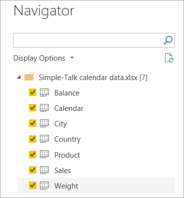
To work through the examples in this article, you’ll need to download the worksheets from this workbook. Tick the following worksheets to load data from this workbook into a new Power BI report:

Now create a relationship between the Calendar and Sales tables by the SalesDate column, as follows (note that initially the Balance and Weight tables aren’t linked to any others):

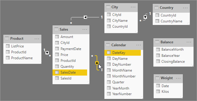
NOTE: This article assumes that you are only concerned with the date when sales are made. If you wanted to be able to choose between the sales date and the payment date when analysing data, you’d either have to create multiple versions of the Calendar table or multiple relationships, as described in the previous article in this series.

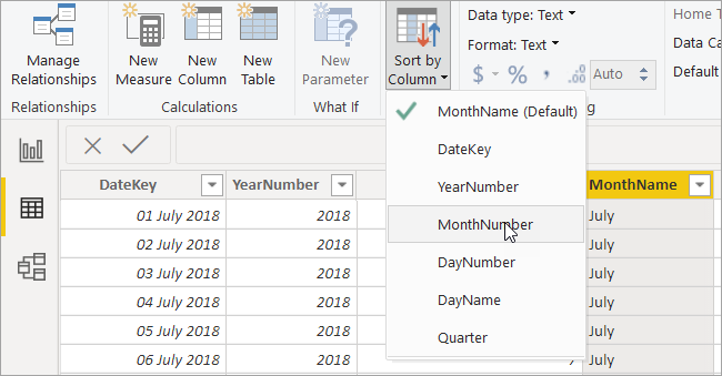
Finally, switch to the Modeling ribbon and choose to sort the month name by the month number:

And make the YearNumber a text column:

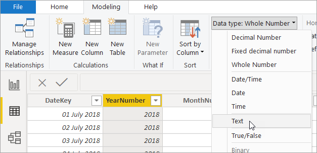
Again, the reason for both of these changes is covered in the previous article in this series.

Creating a Draft Matrix

To accommodate all the wonderful measures that you’re going to bring into being, create a matrix visual to show total amount sold by year and month:

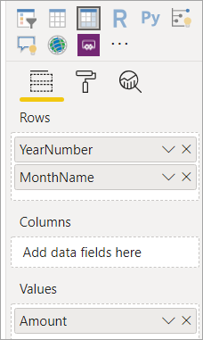
I think it’ll be easier to work with if you have all 12 months appearing, so choose to show months even when they have no corresponding data:

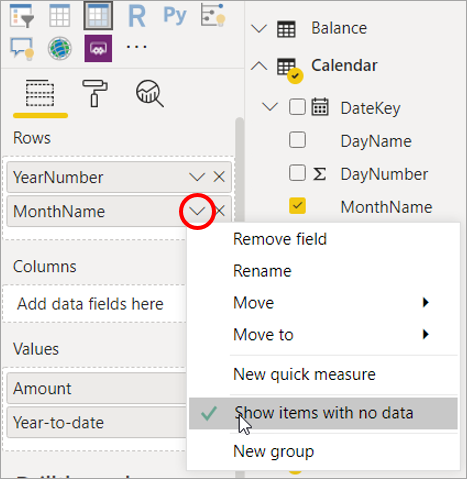
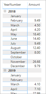
Here’s what the start of the matrix should look like:

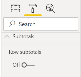
I’ve decided to hide the row subtotals for the matrix. To turn these off, go to the formatting tab and look under the Subtotals section for Row subtotals.

If for any reason you don’t get the +/- icons to expand/collapse rows, enable this setting in the matrix’s formatting properties:

How Time-intelligence Functions Work

To begin with, create a new measure on the Sales table to show total sales to date for each year (don’t worry too much yet about how this works):

Year-to-date = CALCULATE(
    SUM(Sales[Amount]),
    DATESYTD('Calendar'[DateKey])
)

I’ll come back to the DATESYTD function in more detail later in this article, but for the moment I want to use it as an example to explain how any DAX time-intelligence function is calculated. Here’s what this measure should show for the matrix:

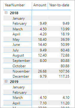
What I want to do is to focus on one figure – the year-to-date sales for March 2018. Start by looking at the sales amount for March 2018, which is 4.50:

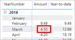
The filter context for this figure is all of the dates in March 2018:

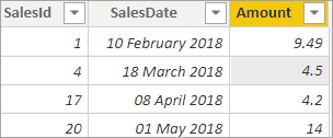
There’s only one sale in March 2018, so that’s why you get 4.50 as the sales for the cell:

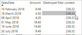
By contrast, the measure to calculate year-to-date sales first destroys the existing filter context for the sales date. Without any additional change, you would get the same figure for each month:

However, the measure then replaces the filter context with one which picks out all of the dates from the calendar table which are on or before 31^st March in 2018:

Year-to-date = CALCULATE(
    SUM(Sales[Amount]),
    DATESYTD('Calendar'[DateKey])
)

The filter context is now as follows for the cell:

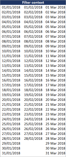
Power BI knows when days, months, quarters, and years start and end (they’re called time-intelligence functions for a reason!). Curiously, Power BI doesn’t know about weeks, so if you want to do weekly reporting, you’ll have to create new aggregator columns yourself in your calendar table (again, the previous article in this series gives a guide for how to do this sort of thing).

Here are the sales figures for the start of 2018:

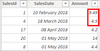
Adding 9.49 and 4.5 gives the year-to-date figure of 13.99! This is what every time-intelligence function does: it destroys the previous filter context for each value in a visual’s underlying data and replaces it with a different one according to the combination of DAX functions you’ve chosen.

Period to Date Functions

Now to take a look in detail now at how to do specific things, beginning with calculating yearly, quarterly or monthly cumulative figures. You can do this using one of these functions:

• DATESYTD or TOTALYTD (year-to-date)
• DATESQTD or TOTALQTD (quarter-to-date)
• DATESMTD or TOTALMTD (month-to-date)

This functionality is typical of time-intelligence functions in DAX: there are often two or three ways to do the same thing, and which one you use is a matter of personal preference. Here’s a function giving the year-to-date figures using DATESYTD shown earlier:

Year-to-date = CALCULATE(
    // you could use a different aggregation function
    SUM(Sales[Amount]),
    // calculate over the dates for the year-to-date
    DATESYTD('Calendar'[DateKey])
)

Here’s a function to do exactly the same thing using TOTALYTD:

Year-to-date 2 = TOTALYTD(
    // again, we could use MAX, MIN, COUNT, etc. here
    SUM(Sales[Amount]),
    'Calendar'[DateKey]
)

These two measures should give the same figures because they are, after all, doing exactly the same thing:

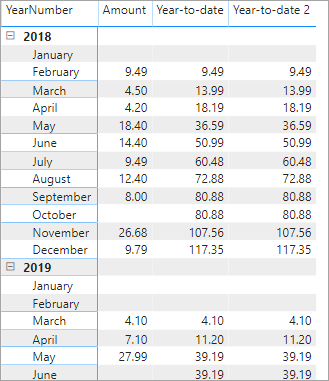
I prefer the first measure since it’s clearer what it’s doing (destroying the existing filter context, and replacing it with one which uses the dates for the current year up to and including the last day in the current period). The second measure using TOTALYTD is just a convenient shorthand for this.

Coping with Different Financial Year-ends

Not everyone’s financial years end conveniently on 31^st December, so you can specify a second argument for the DATESYTD function, giving your year-end date in the format DD-MM:

As an example, suppose that your year ends on 31^st March. Then you could use this measure:

Year-to-date = CALCULATE(
    // you could use a different aggregation function
    SUM(Sales[Amount]),
    // calculate over the dates for the year-to-date,
    // but with year ending on 31st March
    DATESYTD('Calendar'[DateKey],"31-03")   
)

This measure would give this report (the box shows how the figures from 1^st April 2018 to 31^st March 2019 are calculated):

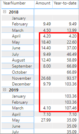
This result would look much better if you created a new aggregator column to give the financial year and reported by that. An idea of how to do this is shown in the previous article in this series. Since I’m feeling charitable, here is the formula that you could use to create a new calculated column in your Calendar table for the financial year:

Financial year = IF(
    [MonthNumber] <= 3,
    // for dates up to and the end of March
    [YearNumber] - 1 & "-" & [YearNumber],
    // for dates from April to December
    [YearNumber] & "-" & [YearNumber] + 1
)

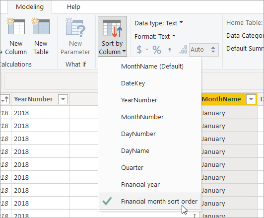
You’ll also need a formula to determine how to sort months, so that April comes first and March last:

Financial month sort order = IF(
    [MonthNumber] <= 3,
    // for dates up to and the end of March
    [MonthNumber]+12,
    // for dates from April to December
    [MonthNumber]
)

You can then choose to sort your months by the Financial month sort order column you’ve created:

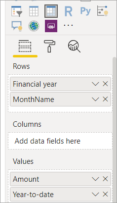
If you then display the financial year column you’ve created in your matrix instead of the year, like this:

You should now get something a lot less confusing:

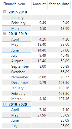
This may seem like a lot of faff, but remember that you’ll only have to set up the calculated columns in your calendar once and once only.

Finally, on the subject of changing your year-end dates, I’ve only shown so far how to change the financial year-end using the DATESYTD function. The process for the TOTALYTD function is similar, but there is a catch. Here’s the syntax:

So it looks for all the world as if the argument to set a new year-end date is the fourth one, and that if you’re not setting any additional filter, you will need to find some way to omit the third argument. However, this measure works:

Year-to-date 2 = TOTALYTD(
    // again, we could use MAX, MIN, COUNT, etc. here
    SUM(Sales[Amount]),
    'Calendar'[DateKey],
    // change the year-end date
    "03-31"
)

Somehow Power BI works out that you’ve missed out the third Filter argument. In every other Microsoft product I’ve used, you need to use a comma placeholder to show that you’re omitting an argument to a function, but if you try to do this in the formula above you get an error!

If you’re wondering which functions support the additional year-end argument, the answer is all those for which this would be relevant – here’s the list for reference:

Functions	What they do
STARTOFYEAR, ENDOFYEAR	Return the first or last date in the year for the current filter context.
PREVIOUSYEAR, NEXTYEAR	Return a table of the dates in the previous or next year, based on the current filter context’s latest date.
DATESYTD, TOTALYTD	As covered on the previous page!
OPENINGBALANCEYEAR, CLOSINGBALANCEYEAR	Return the opening or closing balance on the first/last day of the year for the current filter context.

Referencing Previous Periods

Suppose that you want to show for each day, month, quarter or year what your sales were in the same period twelve months ago? Again, there are two ways (at least) to do this:

• Using the DATEADD function
• Using the SAMEPERIODLASTYEAR function

The DATEADD function is more useful, as it can also show sales 13 months ago, or four years ago or indeed any number of periods of any type ago, but I’ll explain both functions in the interest of fairness. Start by showing for each month the sales in that month against the sales in the same month in the previous quarter, which should give this:

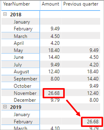
Note that I’ve reverted to using the typical calendar month and year in the matrix, and I’m sorting the calendar months by the MonthNumber column again.

So, for example, the measure should show previous quarter sales for February 2019 as 26.68, since these were what the sales were three months earlier for the same period. You can’t use the SAMEPERIODLASTYEAR function to do this for obvious reasons (the clue’s in the name), and for some strange reason there isn’t an equivalent SAMEPERIODLASTMONTH or SAMEPERIODLASTQUARTER function, so instead, you’ll use the versatile DATEADD function. This takes three arguments:

The arguments are:

1. The calendar dates, as usual
2. The number of intervals to go forward in time
3. The interval to use

Here’s what you’ll see for the third argument when typing it in:

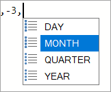
For this example, you can either go three months back in time or one quarter; it makes no difference which you choose. I’ve gone for three months, to produce this measure:

Previous quarter = CALCULATE(
    SUM(Sales[Amount]),
    // go back 3 months (could have used -1 QUARTER)
    DATEADD('Calendar'[DateKey],-3,MONTH)
)

Since the DATEADD function is so powerful (you can go forward or backwards in time, using days, months, quarters or years as the time interval), it seems pointless having the SAMEPERIODLASTYEAR function as a shortcut for it. Nevertheless, it exists! To illustrate it, switch to showing for each period what sales were 12 months (i.e. one year) previously. You could solve this using this measure:

Previous year 1 = CALCULATE(
    SUM(Sales[Amount]),
    SAMEPERIODLASTYEAR('Calendar'[DateKey])
)

Or this measure:

Previous year 2 = CALCULATE(
    SUM(Sales[Amount]),
    DATEADD('Calendar'[DateKey],-1,YEAR)
)

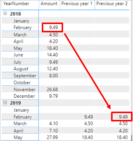
To prove this, here are both measures in the matrix, showing that they both return 9.49 against February 2019, since that’s what sales were for the corresponding period 12 months previously:

Getting the Whole of a Previous Period

The functions above return a figure for a corresponding period, but what happens if you want to get sales for the whole of the previous period? To see what this means, consider this example (it shows year-to-date figures as a fraction of total sales for the whole of the previous year):

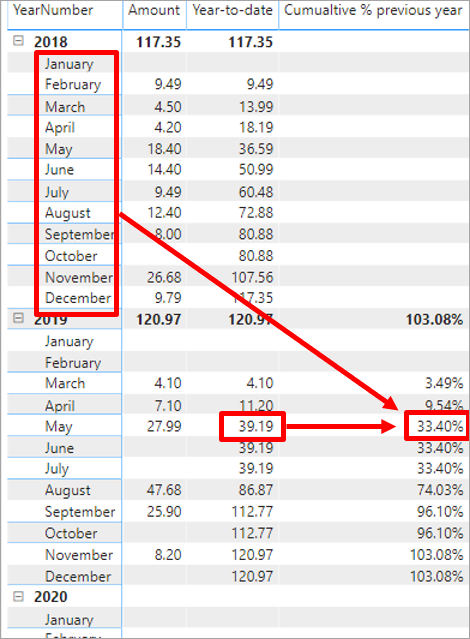
The figure shown for May 2019 (boxed above) is 33.40%, since year-to-date sales at this point are 39.19, and sales for the whole of the previous 12-month period were 117.35. 39.19 divided by 17.35 gives 33.40%. The fact that by the end of 2019, the sales have exceeded 100% of the sales for the whole of the previous year is presumably a good sign!

To calculate this measure, use the PARALLELPERIOD function. This has the same format as the DATEADD function but returns the aggregate figure for the whole of a previous period, rather than for the period corresponding to the one you’re viewing. The syntax of the function is as follows:

The interval can be any one of the following:

Note that unlike for the DATEADD function you can’t use the PARALLELPERIOD function to return the aggregate of a number for the whole of the previous day, presumably because this is at too low a level of granularity.

Putting all this together, here’s how the measure to give the figures above might read:

Cumulative % previous year = DIVIDE(
    // divide the year-to-date figure …
    CALCULATE(
        SUM(Sales[Amount]),
        DATESYTD('Calendar'[DateKey])
    ),
    // … by sales for the whole of the previous year
    CALCULATE(
        SUM(Sales[Amount]),
        PARALLELPERIOD('Calendar'[DateKey],-1,YEAR)
    )
)

That is: divide year-to-date sales by sales for the whole of the previous year.

To format the measure, select it in the list of fields. Then, on the Modeling ribbon, format as a percentage with two decimal places.

Moving Averages

Moving averages are one of the most useful ways to show trends, since they iron out any seasonal effects. Sadly, there is no MOVINGAVERAGE function in DAX, but you can create your own expression in a couple of different ways, of which I’ve shown the one I believe to be the more useful below.

To illustrate moving averages, first create a relationship between the Weight and the Calendar tables:

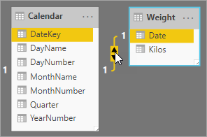
The Weight table is a bit of an anomaly – it doesn’t have anything to do with the others. I’ve been recording my weight roughly every week for the last couple of years, to see if it’s going up or down. Although this is slightly obsessive behaviour, it does provide a perfect example of the use of moving averages.

Add a calculated column to the Calendar table:

The new column should use this formula:

YearMonth = [YearNumber] &"-"& if([MonthNumber]<10,"0","") 
    & [MonthNumber]

This column should return the year number and month number for each calendar date, which you can then use to display as labels on a chart:

Now create a line chart showing the average of the Kilos field from the Weight table against the YearMonth field from the Calendar table:

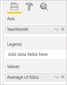
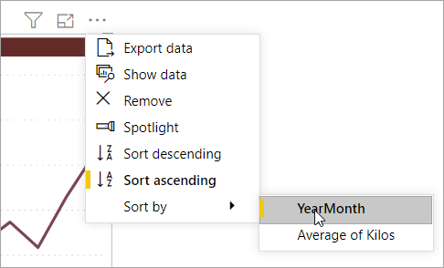
Make sure that you choose to show the average kilos, not the default sum. Also, you will need to sort your chart by the YearMonth field, not by the average kilos (the default):

You should get something like this (I’ve formatted my chart a bit, but it’s the underlying trend which interests us here):

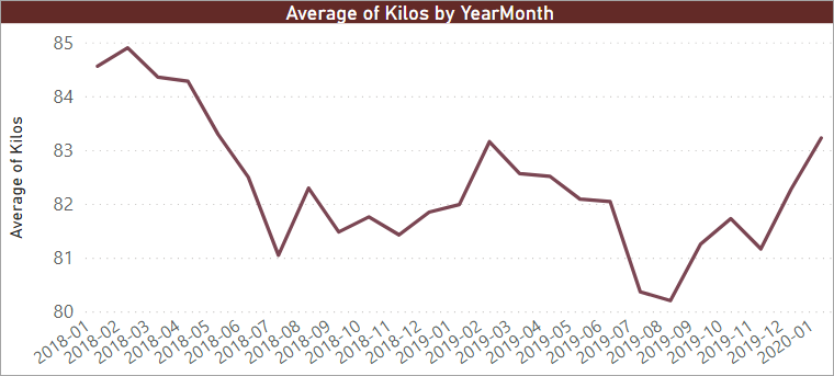
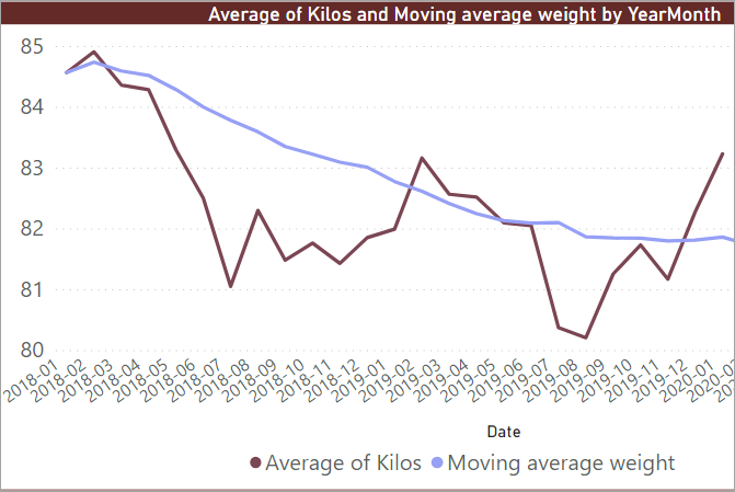
The question is this – is my weight going up or down? To answer this, you have to take account of seasonality –I eat way too much at Christmas but tend to go on family cycling holidays in July during which my weight falls. To show what’s happening, create a 12-month moving average. If this works, the figure for February 2019, for example, should return the average for the previous 12 months (that is for the period March 2018 through to February 2019).

Here’s a measure you could create to show the 12-month moving average:

Moving average weight = CALCULATE(
    -- average weight in kilos ...
    AVERAGE('Weight'[Kilos]),
    
    -- ... over the period between two dates, 
    -- as specified in the arguments
    DATESBETWEEN(
        'Calendar'[DateKey],
        
        -- the first date takes the last date
        -- for the filter context, works out
        -- what the corresponding period would 
        -- have been for the previous year and 
        -- adds one day to the last date of it
        NEXTDAY(
            SAMEPERIODLASTYEAR(
                LASTDATE('Calendar'[DateKey])
            )
        ),
        
        -- the last date is just the end date
        -- for the filter context
        LASTDATE('Calendar'[DateKey])
    )
)

Here’s the chart this would give, and it looks like good news – my weight may be going up and down, but on a seasonally adjusted basis it’s falling steadily, if slowly:

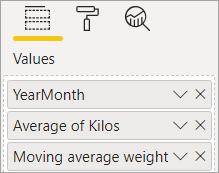
To understand how the measure works, create a table to include these fields:

This table should show the following data (I’ve added the red box separately – you obviously won’t be able to create this in Power BI):

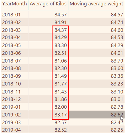
The 12-month moving average for February 2019 is 82.62 and is shown selected above. This is the average of the figures for the 12 months shown in the red box. To see how the measure arrives at this figure, start in the middle of it:

LASTDATE('Calendar'[DateKey]

This expression would return 28^th February 2019 for the above example (being the last date in the date filter context period for the month under consideration). Now add the next bit of the measure:

SAMEPERIODLASTYEAR(
    LASTDATE('Calendar'[DateKey])
)

This expression will give 28h February 2018, being the corresponding date in the previous calendar year. Expand the measure a bit more and you get:

NEXTDAY(
SAMEPERIODLASTYEAR(
     LASTDATE('Calendar'[DateKey])
)
)

This expression will give the day following 28^th February 2018 (that is, 1^st March 2018). So the whole date range across which you’re averaging my weight is given by:

DATESBETWEEN(
        'Calendar'[DateKey],
        
        -- the first date takes the last date
        -- for the filter context, works out
        -- what the corresponding period would 
        -- have been for the previous year and 
        -- adds one day to the last date of it
        NEXTDAY(
            SAMEPERIODLASTYEAR(
                LASTDATE('Calendar'[DateKey])
            )
        ),
        
        -- the last date is just the end date
        -- for the filter context
        LASTDATE('Calendar'[DateKey])
    )

This gives the dates between 1^st March 2018 and 28^th February 2019, which was the goal!

Semi-additive Measures

For the last part of this tutorial on using time-intelligence functions, I’ll discuss semi-additive measures (that is, measures which sometimes aggregate data and sometimes don’t). To start, create a new layout in your report, and create this relationship:

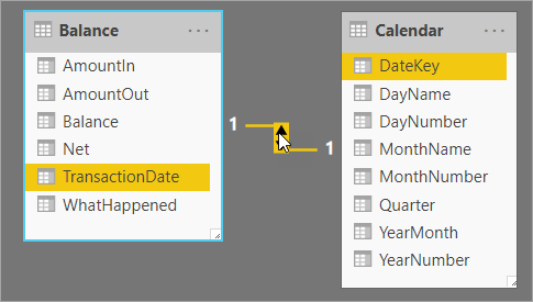
Suppose that the Balance table contains your bank statement for the period July to September 2019. You want to get the closing bank balance at the end of each month, so you create a report based on this Balance table:

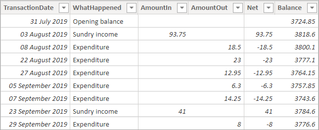
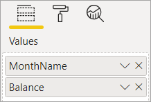
To do this, you add a table with these fields:

You should now see this table (if you include a slicer as shown to look at 2019 data only):

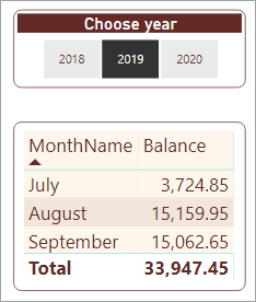
This result is clearly wrong (it would be nice if your bank added your daily balances to get your monthly balance, assuming that you aren’t overdrawn, but life doesn’t work that way). The goal is to pick out the last amount in each month. Fortunately, there is a family of semi-additive DAX functions to draw on:

Function(s)	What the functions do
CLOSINGBALANCEYEAR, CLOSINGBALANCEQUARTER, CLOSINGBALANCEMONTH, OPENINGBALANCEYEAR, OPENINGBALANCEQUARTER, OPENINGBALANCEMONTH	Calculate the value of an expression at the first or last date of the year, quarter or month for the current filter context.
FIRSTDATE, LASTDATE	Return the first or last date for the filter context.
FIRSTNONBLANK, LASTNONBLANK	Return the first or last date for the filter context for which a given expression has a value.

For this example, you could try using the LASTDATE function, with this measure:

Attempt at closing balance = CALCULATE(
    -- work out the total balance ...
    SUM(Balance[Balance]),
    
    -- for the last date in the current
    -- filter context
    LASTDATE('Calendar'[DateKey])
    
)

This formula would give this column in the table:

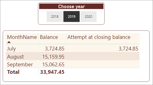
This formula is a bit better, but it only shows figures for July. This is because in the table of balances, there weren’t any transactions on the last dates of August or September in 2019, so the measure is returning blank for these two months. You could get around this by using the clever LASTNONBLANK function, which will return the balance on the last date for which a transaction exists:

Closing balance = CALCULATE(
    // work out the total balance ...
    SUM(Balance[Balance]),
    
    LASTNONBLANK(
    
        // ... for the last date in the current filter context ...
        'Calendar'[DateKey],
        
        // ... for which there are rows in the table of balances
        COUNTROWS(RELATEDTABLE(Balance))
    )   
)

This measure will give the correct closing balances. The function is called semi-additive because you could then aggregate these if you chose, although normally you won’t want to do this:

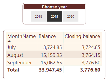
The measure needs a bit of explanation. The syntax of the LASTNONBLANK function is as follows:

The measure returns the total balance for each month on the last day for which there are any corresponding rows in the Balance table. The reason for the RELATEDTABLE function is that at this point in the measure it’s slipped from filter to row context. The LASTNONBLANK function is an iterator function which goes down the rows in the current filter context (for this example, the dates in each month), evaluating for each whether it could be included. Relationships between tables aren’t automatically supported within row context, so you need to use the RELATEDTABLE to bring information in from another table.

It seems appropriate to end with this paragraph about row and filter context, since understanding these two concepts is key to understanding DAX. Thank you for reading through this article, and (perhaps) the other ones in this series, and happy DAXingthe date of the sale If you’ve enjoyed the series, you may like to know that the author’s company Wise Owl Training provide classroom training in Power BI and DAX, although currently only in the UK.

Conclusion

In this article, you’ve learnt that you can override the default filter context for any measure referencing a calendar date column. The replacement filter context could, for example, allow you to return year-to-date figures, show data from the same period in a previous month, quarter or year, or even show totals from prior periods or moving averages. You’ve also learnt how to use semi-additive measures to show closing (and by analogy) opening balances. You should also now have a feel for the fact that time-intelligence functions have this name because DAX has built-in knowledge of how days, months, quarters and years behave.

 

The post Creating Time-Intelligence Functions in DAX appeared first on Simple Talk.

from Simple Talk https://ift.tt/37qjncf
via