Tuesday, June 30, 2020

How to Create a Settings Menu in Unity

Virtually every game you play, especially on a personal computer, allows you to change the graphics settings to get the best performance and appearance you can on your device. These games save those settings and then reload them whenever the user reopens the project. Perhaps you might be wondering how it does all that? In the case of a typical Unity project, this is done by accessing the quality settings and changing the values to match with the player’s selection. Saving those settings is also simple by utilizing the Unity Player Preferences system. This method of saving data and preferences has been discussed before in this article.

Soon to follow is a tutorial showing how you access these parameters and allow the user to change them at their leisure. There are options for selecting a quality preset, where the game automatically chooses settings based on how nice the user wants the game to look, as well as options for setting the game to windowed or fullscreen. They’ll also be able to select the exact anti-aliasing and texture quality preferences they have as well as the resolution and the master volume. While these aren’t all the options the user can change, this article should give any Unity developer an idea of how to create a graphics settings menu.

As there are quite a few moving parts outside of the code, this tutorial is primarily focusing on the coding work involved in making a settings menu. You can use the codeless template below to follow along or recreate the user interface seen in the article yourself. An introduction to creating a user interface is detailed here. The template and complete version of the project also has music included for testing the master volume settings once it is programmed and ready. This music was created by Kevin MacLeod, and more info on it can be found directly below.

Music credit:

Night In Venice by Kevin MacLeod

Link: https://incompetech.filmmusic.io/song/5763-night-in-venice

License: http://creativecommons.org/licenses/by/4.0/

Of course, if you prefer a song from your own computer, feel free to use it. In addition, the project borrows a stone texture created by LowlyPoly. That asset can be viewed in the Unity Asset Store here. This asset is included in both the template and the complete project when downloaded from the links below.

Project Overview

To load an already existing project, click the Add button in the Unity Hub and navigate to the project in the dialog that appears. Select the folder containing the project, then click Select Folder.

First, here’s a quick overview of the project. From the start, you should see an already completed user interface shown in Figure 1, created using Unity’s default assets, with all the settings that can be changed. Next to it is a sphere object with the stone texture applied. This image has been included to help the user better tell the differences between the different settings.

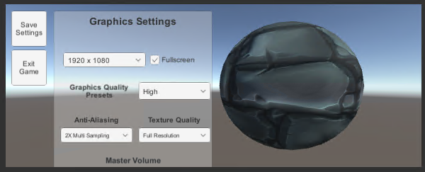
Figure 1: The Graphics Settings menu

The menu should consist of four drop-downs, a checkbox, and a slider. The drop-down for selecting resolutions has a few options already, but they are mere placeholders and can be ignored as Unity is capable of automatically filling in all resolution options available to the user. Options in the other three drop-downs all correspond to their respective Unity graphics settings. It has already been done, but if you were to recreate this menu from scratch, you would need to take care to match the order of drop-down options (except the resolution drop-down) with the order of options seen in the Unity settings. That order can be seen by clicking Edit->ProjectSettings then, in the window that appears (Figure 2), selecting Quality on the right-hand side.

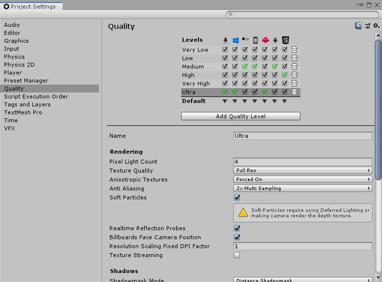
Figure 2: The project’s visual quality settings.

If you wish to set the default quality preset, you can do so by clicking the Default arrows matching with the build type (PC, Android, etc.) and selecting the preset. If downloading the projects from the Github links, the presets will have been modified to give each option more definition. For instance, by default, the Very Low preset’s Texture Quality is at half resolution, but the template has it set to eighth resolution. Feel free to edit them to your liking, but it is not required. You can also see individual settings, such as Texture Quality and Anti Aliasing, further down which this project allows the user to change. There are plenty of other settings here as well, but for the purpose of this tutorial, the options the user can change are limited to just a few. Accessing the other options in code is simple and will be explained in the coding section.

At the bottom is the master volume slider, which works a little differently from the other settings. Manipulating this slider changes the volume of the MainAudio audio mixer seen in the Assets window. If you were to double-click this asset, the Assets window would change to an Audio Mixer window where you could change audio settings from there. If building all this from scratch, you would create an audio mixer using right-click context menu in the Assets window, expose the Volume parameter, then link that with the AudioSource game object with the Output field.

Finally, there are two buttons on the left side of the menu, one for saving settings and one for closing the game. Between these two buttons, the save button is where most of your attention will go. As mentioned above, the Player Preferences system is used to save graphics settings. When the user reloads the project, any settings they saved are loaded according to their saved preferences.

Feel free to click around the editor and check out the other objects hidden under UI in the Hierarchy to get a better feel for what all the different objects are. When you’re ready, double-click the SettingsMenu script asset in the Assets window to begin the coding process.

SettingsMenu

To start, you’ll need the following using statements to accomplish everything this project sets out to do. Most of these should appear at the top of the script by default, but, to be safe, each one is listed.

using System;
using System.Collections.Generic;
using UnityEngine;
using UnityEngine.Audio;
using UnityEngine.UI;

Within the class itself, you’ll need to be able to reference many of the objects within the settings menu. You also need to be able to change the volume of the audio mixer. Finally, two private variables are declared. The first is a float called currentVolume, which, as the name implies, stores the current volume. This variable primarily exists for saving purposes, since it’s unfortunately not easy to get the current volume of the MainAudio mixer. Next comes an array of resolutions. Remember when it was said that Unity automatically detects the possible resolutions for a user and fills out the drop-down from there? Those resolutions will be stored inside this array to be used later.

public AudioMixer audioMixer;
public Dropdown resolutionDropdown;
public Dropdown qualityDropdown;
public Dropdown textureDropdown;
public Dropdown aaDropdown;
public Slider volumeSlider;
float currentVolume;
Resolution[] resolutions;

Finally, the default Update method can be commented out or deleted, but keep the Start method. You’ll be coming back to this method later.

Now comes the time to begin properly coding the different methods that make this menu tick. A good place to start would be the SetVolume and SetFullscreen methods.

public void SetVolume(float volume)
{
        audioMixer.SetFloat("Volume", volume);
        currentVolume = volume;
}
public void SetFullscreen(bool isFullscreen)
{
        Screen.fullScreen = isFullscreen;
}

As you can see, the act of changing the settings is quite simple. In both methods, the actual change is occurring in just a single line. With SetVolume, you get the audioMixer's SetFloat method and pass in the volume parameter. How does Unity get this value? In the editor, the volume slider is given this method for its OnValueChanged event. In doing so, the slider is told that its current value is passed into SetVolume's volume parameter, thus providing the audioMixer with the new master volume value to be changed to. Finally, currentVolume is given the value of volume to hang onto whenever the user saves their settings.

SetFullscreen has the same idea, but with one less line of code. Additionally, it also gets the Unity Screen class, and then the fullScreen boolean variable from there. Like with SetVolume, the fullScreen value is changed according to the value passed into the isFullscreen parameter, which gets its value from whatever the current value of the FullscreenToggle checkbox in the user interface.

Next up is SetResolution, which puts the resolutions array declared earlier to use:

public void SetResolution(int resolutionIndex)
{
        Resolution resolution = resolutions[resolutionIndex];
        Screen.SetResolution(resolution.width, 
              resolution.height, Screen.fullScreen);
}

Similar to the previous two methods, SetResolution uses a value passed in from the corresponding drop-down. The current resolution is then set using the resolutionIndex parameter, before passing the exact width and height of that resolution into Screen's SetResolution method.

The next two methods, SetTextureQuality and SetAntiAliasing are similar to each other in that they both call the QualitySettings class and change a value within that class. In addition, they both get the quality preset drop-down choice and set it to the value of six, which in this case would be the “custom” option.

public void SetTextureQuality(int textureIndex)
{
        QualitySettings.masterTextureLimit = textureIndex;
        qualityDropdown.value = 6;
}
public void SetAntiAliasing(int aaIndex)
{
        QualitySettings.antiAliasing = aaIndex;
        qualityDropdown.value = 6;
}

Speaking of the quality presets, the last major method for this settings menu is for the quality preset drop-down. This one has a few more steps to it than the others, but the reasons are a little strange. If you changed the quality settings presets when in the Project Settings window, you may need to adjust these values.

public void SetQuality(int qualityIndex)
{
        if (qualityIndex != 6) // if the user is not using 
                               //any of the presets
                QualitySettings.SetQualityLevel(qualityIndex);
        switch (qualityIndex)
        {
                case 0: // quality level - very low
                        textureDropdown.value = 3;
                        aaDropdown.value = 0;
                        break;
                case 1: // quality level - low
                        textureDropdown.value = 2;
                        aaDropdown.value = 0;
                        break;
                case 2: // quality level - medium
                        textureDropdown.value = 1;
                        aaDropdown.value = 0;
                        break;
                case 3: // quality level - high
                        textureDropdown.value = 0;
                        aaDropdown.value = 0;
                        break;
                case 4: // quality level - very high
                        textureDropdown.value = 0;
                        aaDropdown.value = 1;
                        break;
                case 5: // quality level - ultra
                        textureDropdown.value = 0;
                        aaDropdown.value = 2;
                        break;
        }
        
        qualityDropdown.value = qualityIndex;
}

To start, you first check if the user selected the “custom” option. If they did, then there would typically be no reason to change the settings because the user is indicating they want to tweak the individual values themselves. But otherwise, the game sets the quality level preset to the user’s selection. Next comes a switch statement that changes the values of the texture quality and anti-aliasing drop-down boxes depending on which option the user selected.

Why bother with this? It is, admittedly, a little inelegant. This is done to update the drop-downs to show what the option is currently set to in code after selecting the preset. Without it, the drop-downs would show incorrect information. It would be inaccurate to say anti-aliasing is disabled when the “ultra” option is chosen without changing some information in the editor itself. On top of that, at the very end of the method, the qualityDropdown value is set to qualityIndex. What’s the point when the user already selected this? When changing the values of the texture quality and anti-aliasing drop-downs, the SetAntiAliasing and SetTextureQuality methods wind up being called. Remember that they’re called whenever the value is changed. When this happens, the quality preset menu changes to say “custom” which would not be correct in this instance, so it sets the drop-down to show what the user actually selected. It looks like the code runs the risk of firing over and over again due to all the value changes, but in testing this code, nothing of the sort occurred. As mentioned, though, it is a little “hacky.”

With all these methods created, the user can now change their game’s settings to their liking. Now you just need to permit them to save the settings and exit the game. In addition, the project needs to be able to load the saved settings. Best to start with the two remaining buttons. The exit game button is very simple, as it only has one line of code. Saving, on the other hand, is a little more involved.

public void ExitGame()
{
        Application.Quit();
}
public void SaveSettings()
{
        PlayerPrefs.SetInt("QualitySettingPreference", 
               qualityDropdown.value);
        PlayerPrefs.SetInt("ResolutionPreference", 
               resolutionDropdown.value);
        PlayerPrefs.SetInt("TextureQualityPreference", 
               textureDropdown.value);
        PlayerPrefs.SetInt("AntiAliasingPreference", 
               aaDropdown.value);
        PlayerPrefs.SetInt("FullscreenPreference", 
               Convert.ToInt32(Screen.fullScreen));
        PlayerPrefs.SetFloat("VolumePreference", 
               currentVolume); 
}

As promised, the Player Preferences are being used to save the user’s preferred settings. Doing so requires creating a key with an attached value. The key can be named anything you like, and the value comes from any variable. In this case, each key is a string with a name that corresponds to its setting, and the current option selected in the various drop-downs are assigned to those keys. The last two keys, FullscreenPreference and VolumePreference, are a little different from the others. Since Screen.fullScreen is a boolean, you need to convert it to an integer. This is because Player Preferences can only save an integer, float, or string. Meanwhile, VolumePreference, a float, is simply being given the currentVolume variable you’ve been hanging on to.

The next method, LoadSettings, is very much like SaveSettings but in reverse. Using Player Preferences, you search for a key with a matching name. If there is one, you get the value of that key and assign it to the drop-down value. And since the game settings change the moment their corresponding menu values change, the graphics and volume settings changes immediately according to the user’s saved preferences. Of course, if there is no saved setting, then a default value is assigned.

public void LoadSettings(int currentResolutionIndex)
{
        if (PlayerPrefs.HasKey("QualitySettingPreference"))
                qualityDropdown.value = 
                     PlayerPrefs.GetInt("QualitySettingPreference");
        else
                qualityDropdown.value = 3;
        if (PlayerPrefs.HasKey("ResolutionPreference"))
                resolutionDropdown.value = 
                     PlayerPrefs.GetInt("ResolutionPreference");
        else
                resolutionDropdown.value = currentResolutionIndex;
        if (PlayerPrefs.HasKey("TextureQualityPreference"))
                textureDropdown.value = 
                     PlayerPrefs.GetInt("TextureQualityPreference");
        else
                textureDropdown.value = 0;
        if (PlayerPrefs.HasKey("AntiAliasingPreference"))
                aaDropdown.value = 
                     PlayerPrefs.GetInt("AntiAliasingPreference");
        else
                aaDropdown.value = 1;
        if (PlayerPrefs.HasKey("FullscreenPreference"))
                Screen.fullScreen = 
        Convert.ToBoolean(PlayerPrefs.GetInt("FullscreenPreference"));
        else
                Screen.fullScreen = true;
        if (PlayerPrefs.HasKey("VolumePreference"))
                volumeSlider.value = 
                    PlayerPrefs.GetFloat("VolumePreference");
        else
                volumeSlider.value = 
                    PlayerPrefs.GetFloat("VolumePreference");
}

Finally, it’s time to return to the Start method left alone earlier. All remaining code from here on goes inside this method. As mentioned before, Unity is capable of getting a list of all possible resolution options available to the user and filling in the resolution drop-down with those options. To do that, you first need to clear the placeholder list, create a new list of strings, and set the resolutions array to hold all the possible resolutions available. In addition, you’ll also create a new integer named currentResolutionIndex for use in selecting a resolution that matches the current user’s screen.

resolutionDropdown.ClearOptions();
List<string> options = new List<string>();
resolutions = Screen.resolutions;
int currentResolutionIndex = 0;

In order to find a matching resolution and assign it, you’ll need to loop through the resolutions array and compare the resolution width and height to the user’s screen width and height to find a match. While you’re at it, you’ll also add every resolution option to the options list.

for (int i = 0; i < resolutions.Length; i++)
{
        string option = resolutions[i].width + " x " + 
             resolutions[i].height;
        options.Add(option);
        if (resolutions[i].width == Screen.currentResolution.width 
          && resolutions[i].height == Screen.currentResolution.height)
                currentResolutionIndex = i;
}

With the list created and a matching resolution found, the only task remaining is to update the resolution drop-down with the new options available and call LoadSettings to load any saved settings. You’ll also pass in currentResolutionIndex into LoadSettings to be used in case a saved resolution preference was not found.

resolutionDropdown.AddOptions(options);
resolutionDropdown.RefreshShownValue();
LoadSettings(currentResolutionIndex);

Adding this code not only completes the Start method, but also completes the entire script. While many of the individual methods act similarly to each other, the specifics are a little different with each one, thus creating a lot to go through. However, this code won’t do anything without being assigned to the different user interface elements first. Complete that, and the project will be finished. Remember to save your work if you haven’t already!

Final Tasks

To assign the different methods to their respective UI elements, you first must make sure the UI object is expanded to show all child objects in the Hierarchy. This is done by clicking the small arrow next to the UI object. From here, the process for assigning methods to menu elements is largely the same for each element. The following assigns the ResolutionDropdownMenu object to its respective method. First, select the object and scroll down in the Inspector window until you find the On Value Changed event list. Once found, click the small plus button on the lower right corner of the list to add a new event as shown in Figure 3.

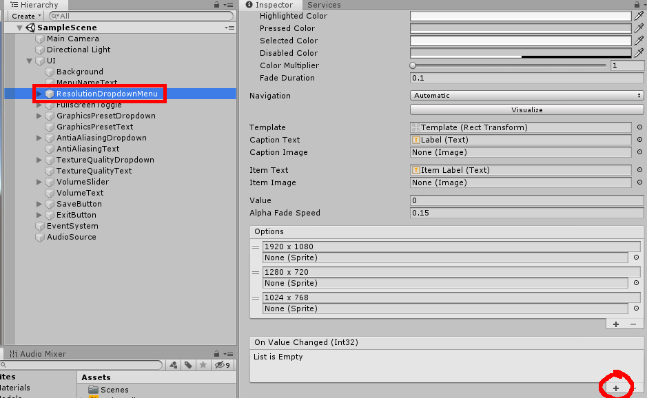
Figure 3: Creating a new On Value Changed event.

Click and drag UI from the Hierarchy into the object field. Doing this allows you to use functions from the SettingsMenu script currently attached to UI. Note that the template should have the SettingsMenu attached in advance. If doing from scratch, you’d simply select UI and drag the SettingsMenu script onto it as shown in Figure 4.

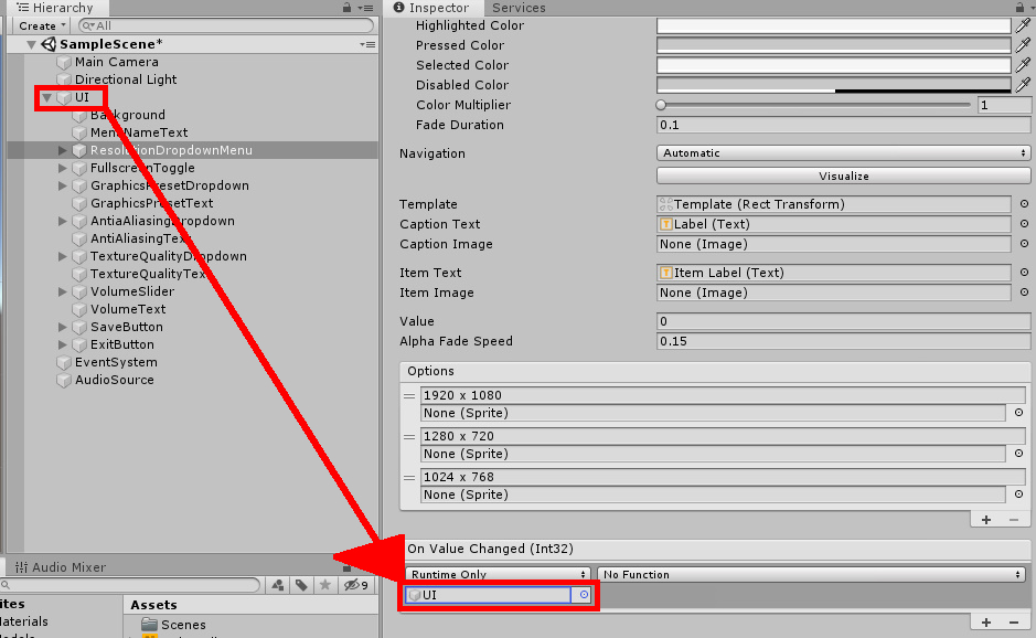
Figure 4: Setting the object field in the event.

Next, click the drop-down that currently says No Function. Navigate to SettingsMenu to show more options. You’ll need to select the SetResolution option, but there are two of them. Selecting the one under Static Parameters would create a new field in the event list where you can enter input for a parameter. The input changes constantly based on the player’s desires, so a better way to handle this is to select SetResolution under Dynamic Int, which is the top part of the function menu as shown in Figure 5.

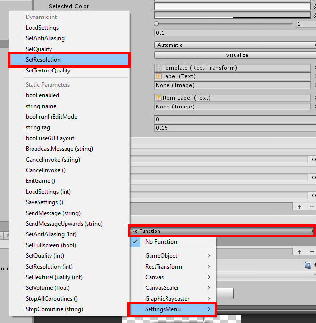
Figure 5: Choosing a function from the Dynamic portion of the submenu.

Everything but the save and exit buttons is set this way. Table 1 below shows all menu elements with their corresponding function. Keep in mind that different elements may show the Dynamic portion of the function list differently. For instance, when setting VolumeSlider’s value change function to SetVolume, you’ll select the function under the Dynamic Float section of the menu.

Object Name

Function

ResolutionDropdownMenu

SetResolution()

FullscreenToggle

SetFullscreen()

GraphicsPresetDropdown

SetQuality()

AntiAliasingDropdown

SetAntiAliasing()

TextureQualityDropdown

SetTextureQuality()

VolumeSlider

SetVolume()

Table 1: All UI elements and their respective functions

As mentioned, the save and exit buttons are set a little different. Instead of adding an On Value Changed event, you’ll be adding an On Click event. Like before, the object the function is pulled from is the parent UI object. When selecting a function, you’ll select SaveSettings() for the save game button and ExitGame() for the exit button. There is no dynamic portion of the submenu to look through, so you should only see one option for the function. Figure 6 has an example of setting a function to a button.

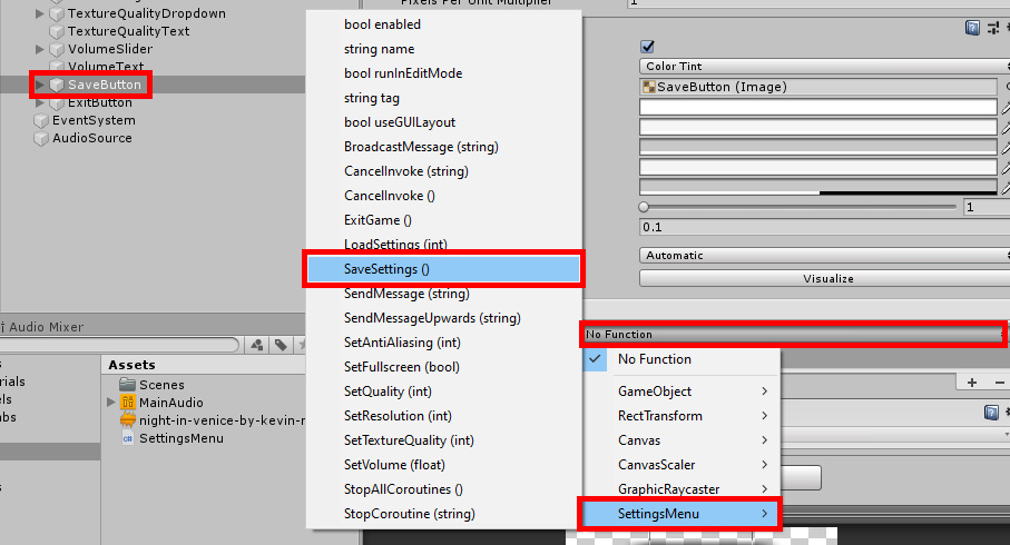
Figure 6: Setting the function for On Click.

The last step before testing is to let SettingsMenu know what all the different drop-downs are as well as the audio mixer and the volume slider. Select the UI object from the Hierarchy and find the SettingsMenu component. Each empty field in the component is given a corresponding object. The Audio Mixer receives MainAudio from the Assets window. All four drop-down fields get a drop-down object (Figure 7), making sure that the given object matches what the field is asking for. For instance, Resolution Dropdown should get the ResolutionDropdownMenu object from the Hierarchy. Finally, the Volume Slider field gets the game object of the same name.

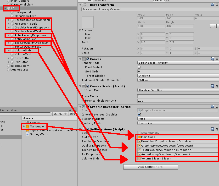
Figure 7: Filling in the empty Settings Menu fields.

While you can test out the project from the editor, you probably won’t be able to see the changes as well, if at all, when selecting different options in the menu. It is recommended you build an exe and play the game from the exe file. To do this, go to File->Build Settings in the top menu. In the window that opens, drag the SampleScene scene from the Scenes folder in the Assets window, into the Scenes In Build box as shown in Figure 8.

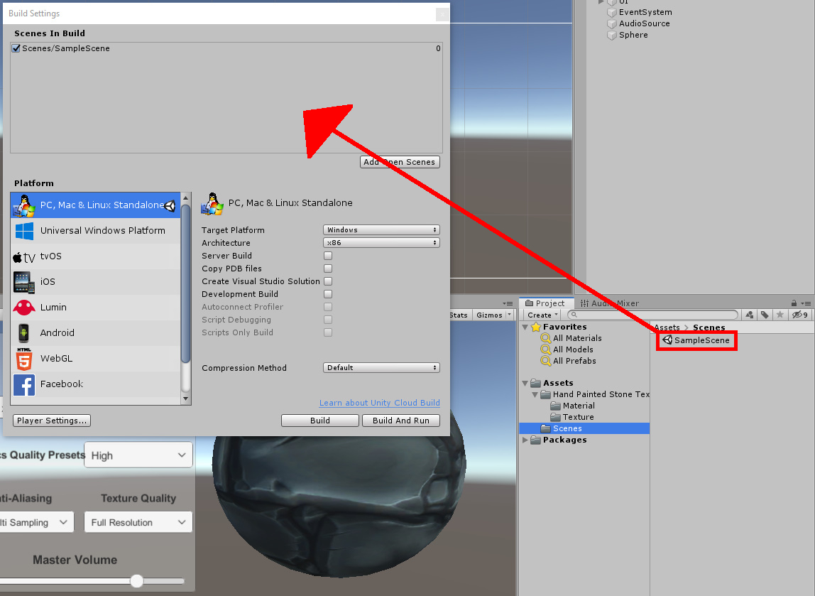
Figure 8: Selecting the scene to build.

Once you’ve done that, click the Build button, choose a build location, then run the game once the build is finished. Try messing around with the different settings and watch as the visuals of the game get higher or lower quality depending on your selection. Over to the right, you should be able to see the Sphere look better or worse, depending on your settings. If changing anti-aliasing, the edges may not be as smooth. Meanwhile, changing the texture quality makes the sphere appear more “grainy.” The differences can be subtle, so an easy way to see these effects is to jump from the Ultra graphics preset to the Very Low preset. You can also adjust the master volume for desired sound output. Note: if for any reason the volume slider appears to be doing nothing, double-check the name of the volume parameter in the audio mixer. You can do this by double-clicking MainAudio in the Assets window, clicking the exposed parameters button, and viewing the list of parameters. There should be one named Volume. If there isn’t, right-click the exposed parameter and rename it, or click the master mixer, navigate to the Inspector, right-click Volume, and select Expose.

Of course, you should also try saving your settings with the save button, closing the game, then reopening to see that your preferred settings have indeed been loaded from the start. Figure 9 shows the app in action.

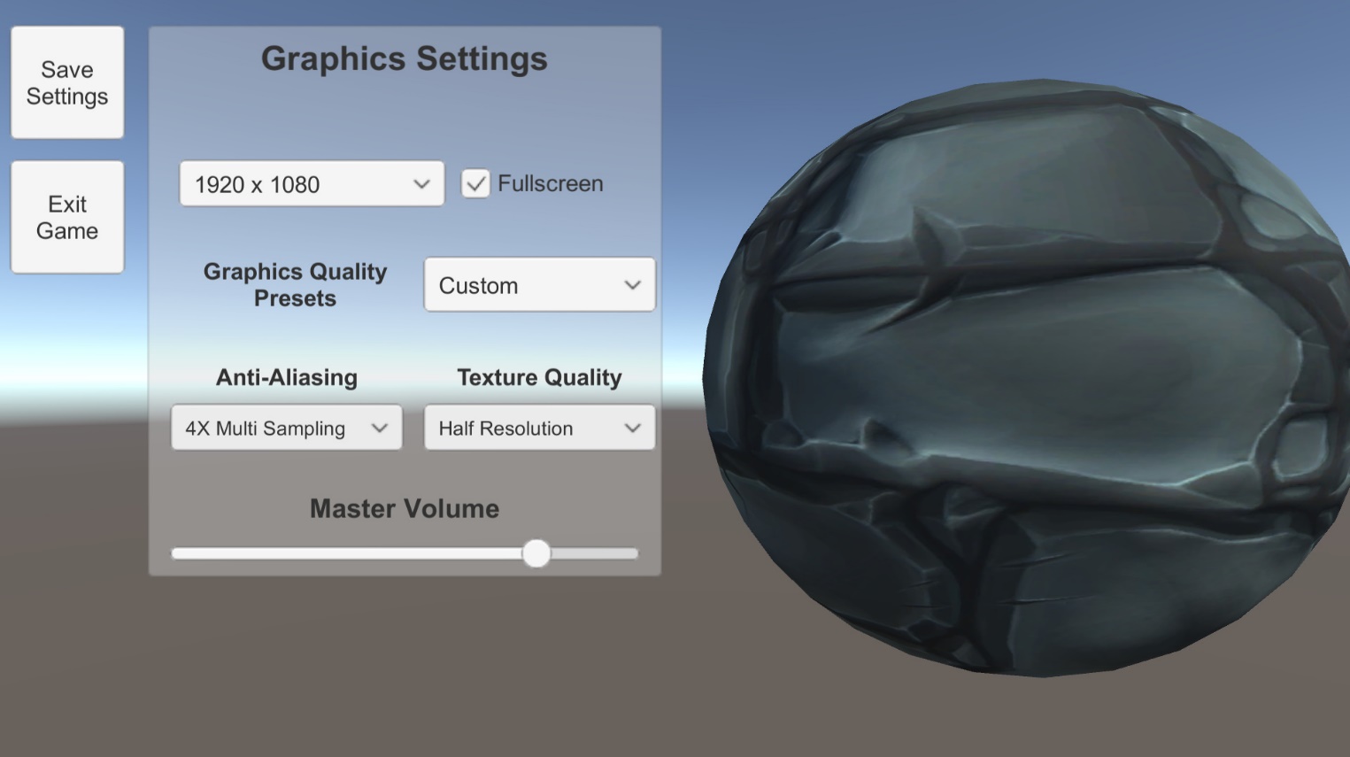
Figure 9: Project in action.

Conclusion

It’s often expected of any game to have some settings that can be tweaked and changed to a user’s liking. The options can be as simple as volume changes or as big as how the game displays its graphics. At first, one may think that creating such a menu for users can be a little challenging, but hopefully, this tutorial should prove that it’s easier than one may think. But why do this in the first place? Imagine a scenario where you have your Unity project you want to put out to the world, but some people don’t have the computer power to run it on normal settings. If you give them the tools to let the game run more smoothly on their machine, even if costs a little prettiness to do it, you give that user a chance to still use your software. In short, creating these options for your users creates the potential to expand your audience.


The post How to Create a Settings Menu in Unity appeared first on Simple Talk.


from Simple Talk https://ift.tt/2VyFPwO
via

The Pros and Cons of Virtual Conferences: Just My Opinions

Before taking any time with the rest of my SQL Saturday Chattanooga, Home Edition teammates to discuss what went right and wrong with our event (it felt mostly right, honestly as far as I could tell, but we won’t totally know until we get the feedback from attendees), I was thinking as I was enjoying the conference process that there were some things about the virtual event that actually were kind of better than the in-person event. Not everything, mind you, I definitely missed seeing everyone which as you will see will be the theme of all of the opinions in this list.

So I am just tossing things into this blog in an outline format with some notes to share from three viewpoints: Attendee, which I did for the SQL Saturday Richmond; Speaker, which I have done a few times both for user group meetings, SQL Saturday Richmond, and another event;  and Organizer which I have so far done with SQL Saturday Chattanooga and am doing with the PASS Summit to a much lesser extent, and maybe another conference.

As an Attendee

  • Pros
    • No travel. Could attend from a smart device, which means you could attend from ANYWHERE. ANYTIME. 
    • Choice. Can choose to go to just one session very economically, even if you were on the road and just stop off at a rest area and catch that session you wanted to see. Could even go to multiple conferences on the same day if they existed.
    • Cost. Can do this all the time, because almost zero expense.
    • Better than purely recordings. While it will also be a con, at least having the ability to ask a few questions with the speakers is awesome. I personally am not a big fan of watching the recordings of many sessions, unless it is something I specifically NEED to know about to solve a problem. In live sessions, I tend to spend time trying to learn new things, because if I get confused, I can ask (often after the session, in the hallway (which was a bit of a con for the virtual conferences so far)  and the speaker can answer or say “go read this”).
    • Video quality over in-person. My home screens is always better than what I can get in most of the free venues (and some of the paid ones.) There is no dependency on some venue screens, lighting, or someone wearing a big had. (One time I presented on a TV smaller than my home TV, from much farther back. I am not complaining, as the conference location was free, but it was interesting!).
    • Ability to do things like closed captioning. Our keynote speaker turned on closed captioning in Powerpoint, something I did not know existed until it was too late to ask people to do. It seems to me that features like this, plus likely improvements in real-time translation could make virtual (or at least, virtual/in-person simultaneous) conferences a better thing some day for some companies
       
  • Cons
    • Limited Interaction. Weak interaction with speakers, limited to moderated chat with the speaker. Using the chat of the GotoMeeting platform (as I have in both SQL Saturday events), meant no hang on afterwards and talk to the person for a while afterwards.
    • Isolation. Once I was done as a speaker, the whole thing felt a bit isolated, like I was in this alone. Being on on Twitter or some social platform helps. But social media usage seems rare among people other than the speakers/people that we all already know. We don’t seem to grow that many people into that community during each new event.

Summary: The learning opportunities are expansive. Some events are live/have to be there events, but some events provide recordings that you can watch pretty much forever. For me, the value in conferences is the social aspects and virtual conferences, once you get too many people to have mics turned on kind of lacks somewhat in the current virtual platforms that smaller virtual conferences can have. Without that social interaction, it can make me lose interest if I have anything else that is pressing, and I am not 100% interested in the material. Even some form of chat environment would be very useful.

The less obvious problem for an attendee is that without this interactive nature, the value of making relationships is gone. Networking and meeting people is one of the most important things we do in the community. Hopefully, the PASS Summit will really get this right, and not only will we be able to have great training, but feel present with the other attendees.

As a Speaker

  • Pros
    • Same as attendee pros. Generally the same as for attendees, cost and travel are minimal. Can do from anywhere needed, anytime. Even during the workday if needed. Video, comfort, etc.
    • Could prerecord. Could be prerecorded in some cases, and just chat along with attendees. This would take the heat off of newer speakers, as they could get the material right, be edited, and just enjoy the moment. 
    • Breadth of reach. It feels good to be a part of something larger than your typical, local area.
  • Con
    • Feedback void. Presenting virtually is like presenting to a mirror. You can see yourself, you can see your slides, but you have no idea what is happening on the other side of the camera. When presenting to a group long-distance, where they are all together, you might be able to occasionally hear from them how it is going. But with 20-100 (or 10000) people in as many locations, who knows what is going on.
    • Connectivity. What if the power goes out (we had a speaker have this happen!) it is really hard for the people on the other side to know what happened. So you really need to be prepared. Prerecording takes this worry out, but does take the spontaneity out (and if you make a mistake, it is in there and you can’t fix it!)
    • Minimal audience interaction. Unless you have a modicum of control over the people in the audience, only chat works. Any attempt to let attendees open their mics tended to end in a mess of feedback and background noise.
       
    • Future limitations? This is speculation, but as time passes, if virtual was the main way conferences were done, there could come a time where the speaking slots were severely limited. A “rockstar” speaker working to get their name around could do 3 or more conferences in a single day, lots more actually based on timezones, because no need to travel. This could really be a thing for people who use this for their primary way of making a living, in that it increases their audience.

Summary: As a speaker, the virtual experience is not terrible, unless you need interaction with the audience. There are two reasons you may need this. Either 1. you are the kind of person who feeds off the energy of the audience or 2. your presentation is very interactive. I did an interactive (using audio) presentation to some local groups, and they were great! We did interactive meetings with 15 speakers, and 20 people in our Disney user group, it was awesome. I did the same SQL presentation to a SQL Saturday group that needed interaction, and it was pandemonium! I switched to chat and it worked well enough, but still was clunky reading the answers (and dealing with grammar that sometimes didn’t say exactly what I thought it did).

Overall though,  as a speaker, the virtual experience is pretty great. It is just different and something to get used to.

As an Organizer

  •  Pros
    • Process seems much easier that in-person.  The big difference is that you need a way to transmit one or more simultaneous sessions. 100 or 1000 is a licensing issue, not a fire-codes issue. You don’t need a venue, you don’t need food.
    • Less liability. No one is physically on site, so no one could get hurt, or really any sort of physically harmed while there. You still need to monitor for bad behavior, slander, racism, etc. But not someone physically assaulting someone.
    • Day of process is shorter. Due to my physical limitations for my entire SQL Server life, I have never been one of the people who carried stuff in and set up the conference. But I have been around to stuff bags a few times, and take tickets early in the morning. This year, we ran four tracks with four people. Each of us in our own houses, and with a slack connection, the web, and GotoMeeting, we were able to manage the entire event. We all arrived at 8am, first session was at 8:30. Last ended around 4:50 or so. We turned off the feed at around 5 and went to dinner with my wife at an outdoor restaurant.
    • More involvement with sessions. As an organizer, I actually felt MORE involved with the conference, because I didn’t end up bouncing around, taking pictures, checking on things, etc. I was able to moderate a room, tweet, and handle other things we had to do pretty easily and still learn a few new things.
    • Weather concerns a bit less acute. Crowd was more dispersed rather than in one location. When it is local, if the weather is good, people will go outside instead of showing up; bad weather and people may stay in; ugly weather and you might even get cancelled and get stuck with a mess. Virtual, everyone is dispersed around the area, and even around the world. And since even your leaders are dispersed you are a lot safer if a leader or two loses power, for example.
  • Cons
    • Social interaction. We did manage to have some, but it was definitely not enough overall. At our event we hosted a virtual speaker meeting the night before, and it was great to just talk with people who dropped in for a few hours. We talked a little about SQL, a bit about set up, but mostly just about “stuff”.  But it wasn’t close to as good as being there in person. Not all speakers came to the meeting, so there were some speakers that I did not even see at all, which was really weird for a conference where I picked the speakers. Usually I would at least be checking to make sure they were all there, and saying hi/thanks.
    • Vendor value. Taking tickets/sharing details with vendors will be a lot harder. So no idea how that would affect future revenue if we need to pay for things like software to enable more socialness.
    • Social interaction. Yep, saying it again. The biggest con is a complete lack of seeing attendees. I didn’t see or hear the voice of any attendee (other than one person who turned their camera on for a minute or two, and one person whose mic was on and their child was screaming so I muted them :))

Summary: I really enjoyed the experience of hosting a virtual event. The process was actually much easier than doing something in-person, and we were able to have the same number of sessions with more people in attendance (and some of our attendees from all around the world (most were from the local area, from our informal poll at the end of the day at least.)

I definitely can see myself participating again some day in a small, medium or large sized virtual conference (even other than the PASS Summit), even once we can start having in-person events. I think that some technologies like closed captioning and real-time translation could make virtual/simultaneous virtual/in-person conferences the wave of the future and better than just in-person. And if we can get the ability to talk in small groups and move from group to group more naturally, it might be better overall anyhow.

The virus has already pushed working at home from something a few of us on the fringe did to something that almost anyone who can does, so why not use it to make conferences better. We just need to make it better to socialize online. I have two thoughts that would really help.

  1. A better chat experience that persists past the end of the conference. Probably currently available for expensive conference suites, but I will start to see what I can find for us small-time operators.
  2. A nice way to have side conferences. For example, say you are in a meeting/presentation, or even it a keynote and you want to ask a question of someone in the room. You click on the person and say “ask for side conversation”, they say yes. Then you could choose:
    1. Chat: Start typing to them (Teams has something like this now. If you are in a meeting, you can click on the person and start a little pop up chat)
    2. Voice: This would be like whispering to each other in the session, but without being annoying to anyone else. Maybe even choose to have the presentation audio playing in one ear, and the side conversation in the other. Cameras could be a part of this too. This would give you that “We are sitting together and being able to say ‘wow’ together live” experience. (Ok, admittedly and probably joke about the salesly-ness of the presentation and discuss better sessions to go to. But at least you wouldn’t be doing this when 100 other people are entranced by it!)

It is definitely a brave new world!


The post The Pros and Cons of Virtual Conferences: Just My Opinions appeared first on Simple Talk.


from Simple Talk https://ift.tt/2YI3lt2
via

Saturday, June 27, 2020

Will We Still be Talking About DevOps in Two Years?

While individual buzzwords will come in and out of fashion, the ideas at the heart of DevOps aren’t going anywhere. 

Like any good buzzword, DevOps may mean different things to different people. There are several good definitions of DevOps out there. My favorite definition comes from @IanColdwater, who defined DevOps in terms a teenager would understand:

Devops is a set of ideas about how process, tools, and people can engineer software better

I love this definition because it doesn’t focus on existing assumptions about what “development” and “operations” are or should be — the point of DevOps isn’t to stick with those old definitions, but instead to evolve our own ideas about how we can create software in ever-better ways.

This evolution isn’t simply implementing automation: instead these ideas involve changes in people’s roles, process definitions, and the tools which are used.

I can easily remember a time before I heard the words “digital transformation,” and I feel that term is already starting to lose popularity. There may be similar fatigue around the term “DevOps.” In two years, we may find ourselves using that word less. But even if this is the case, I’m confident that in two years we will still be building on the set of ideas central to DevOps about how to engineer software better.

This set of ideas includes focal points of being customer centric, maintaining a steady flow of work, and reducing toil. Work in these areas improves code quality, reduces time to market, and focuses individual contributors on value-added-work which many find more enjoyable than repeatable tasks. These results are attractive both to leadership and to employees across the organization.

Even if the specific word “DevOps” falls out of fashion, the set of ideas it embraces are well positioned to stay at the heart of technical initiatives and efforts for well beyond the next two years.


Commentary Competition

Enjoyed the topic? Have a relevant anecdote? Disagree with the author? Leave your two cents on this post in the comments below, and our favourite response will win a $50 Amazon gift card. The competition closes two weeks from the date of publication, and the winner will be announced in the next Simple Talk newsletter.

The post Will We Still be Talking About DevOps in Two Years? appeared first on Simple Talk.


from Simple Talk https://ift.tt/2VmFWLG
via

Thursday, June 25, 2020

Hands-On with Columnstore Indexes: Part 2 Best Practices and Guidelines

The series so far:

  1. Hands-On with Columnstore Indexes: Part 1 Architecture
  2. Hands-On with Columnstore Indexes: Part 2 Best Practices and Guidelines

A discussion of how columnstore indexes work is important for making the best use of them, but a practical, hands-on discussion of reality and how they are used in production environments is key to making the most of them. There are many ways that data load processes can be tweaked to dramatically improve query performance and increase scalability.

The following is a list of what I consider to be the most significant tips, tricks, and best practices for designing, loading data into, and querying columnstore indexes. As always, test all changes thoroughly before implementing them.

Columnstore indexes are generally used in conjunction with big data, and having to restructure it after-the-fact can be painfully slow. Careful design can allow a table with a columnstore index to stand on its own for a long time without the need for significant architectural changes.

Column Order is #1

Rowgroup elimination is the most significant optimization provided by a columnstore index after you account for compression. It allows large swaths of a table to be skipped when reading data, which ultimately facilitates a columnstore index growing to a massive size without the latency that eventually burdens a classic B-tree index.

Each rowgroup contains a segment for each column in the table. Metadata is stored for the segment, of which the most significant values are the row count, minimum column value, and maximum column value. For simplicity, this is akin to having MIN(), MAX(), and COUNT(*) available automatically for all segments in all rowgroups in the table.

Unlike a classic clustered B-tree index, a columnstore index has no natural concept of order. When rows are inserted into the index, they are added in the order that you insert them. If rows are inserted from ten years ago, then they will be added to the most recently available rowgroups. If rows are then inserted from today, they will get added on next. It is up to you as the architect of the table to understand what the most important column is to order by and design schema around that column.

For most OLAP tables, the time dimension will be the one that is filtered, ordered, and aggregated by. As a result, optimal rowgroup elimination requires ordering data insertion by the time dimension and maintaining that convention for the life of the columnstore index.

A basic view of segment metadata can be viewed for the date column of our columnstore index as follows:

SELECT
        tables.name AS table_name,
        indexes.name AS index_name,
        columns.name AS column_name,
        partitions.partition_number,
        column_store_segments.segment_id,
        column_store_segments.min_data_id,
        column_store_segments.max_data_id,
        column_store_segments.row_count
FROM sys.column_store_segments
INNER JOIN sys.partitions
ON column_store_segments.hobt_id = partitions.hobt_id
INNER JOIN sys.indexes
ON indexes.index_id = partitions.index_id
AND indexes.object_id = partitions.object_id
INNER JOIN sys.tables
ON tables.object_id = indexes.object_id
INNER JOIN sys.columns
ON tables.object_id = columns.object_id
AND column_store_segments.column_id = 
     columns.column_id
WHERE tables.name = 'fact_order_BIG_CCI'
AND columns.name = 'Order Date Key'
ORDER BY tables.name, columns.name, 
column_store_segments.segment_id;

The results provide segment metadata for the fact_order_BIG_CCI table and the [Order Date Key] column:

Note the columns min_data_id and max_data_id. These ID values link to dictionaries within SQL Server that store the actual minimum and maximum values. When queried, the filter values are converted to IDs and compared to the minimum and maximum values shown here. If a segment contains no values needed to satisfy a query, it is skipped. If a segment contains at least one value, then it will be included in the execution plan.

The image above highlights a BIG problem here: the minimum and maximum data ID values are the same for all but the last segment. This indicates that when the columnstore index was created, the data was not ordered by the date key. As a result, all segments will need to be read for any query against the columnstore index based on the date.

This is a common oversight, but one that is easy to correct. Note that a clustered columnstore index does not have any options that allow for order to be specified. It is up to the user to make this determination and implement it by following a process similar to this:

  1. Create a new table.
  2. Create a clustered index on the column that the table should be ordered by.
  3. Insert data in the order of the most significant dimension (typically date/time).
  4. Create the clustered columnstore index and drop the clustered B-Tree as part of its creation.
  5. When executing data loads, continue to insert data in the same order.

This process will create a columnstore index that is ordered solely by its most critical column and continue to maintain that order indefinitely. Consider this order to be analogous to the key columns of a classic clustered index. This may seem to be a very roundabout process, but it works effectively. Once created, the columnstore index can be inserted into using whatever key order was originally defined.

The lack of order in fact_order_BIG_CCI can be illustrated with a simple query:

SET STATISTICS IO ON;
GO
SELECT
        SUM([Quantity])
FROM dbo.fact_order_BIG_CCI
WHERE [Order Date Key] >= '2016/01/01'
AND [Order Date Key] < '2016/02/01';

The results return relatively quickly, but the IO details tell us something is not quite right here:

Note that 22 segments were read, and one was skipped, despite the query only looking for a single month of data. Realistically, with many years of data in this table, no more than a handful of segments should need to be read in order to satisfy such a narrow query. As long as the date values searched for appear in a limited set of rowgroups, then the rest can be automatically ignored.

With this mistake identified, let’s drop fact_order_BIG_CCI and recreate it by following this set of steps instead:

DROP TABLE dbo.fact_order_BIG_CCI;
CREATE TABLE dbo.fact_order_BIG_CCI (
        [Order Key] [bigint] NOT NULL,
        [City Key] [int] NOT NULL,
        [Customer Key] [int] NOT NULL,
        [Stock Item Key] [int] NOT NULL,
        [Order Date Key] [date] NOT NULL,
        [Picked Date Key] [date] NULL,
        [Salesperson Key] [int] NOT NULL,
        [Picker Key] [int] NULL,
        [WWI Order ID] [int] NOT NULL,
        [WWI Backorder ID] [int] NULL,
        [Description] [nvarchar](100) NOT NULL,
        [Package] [nvarchar](50) NOT NULL,
        [Quantity] [int] NOT NULL,
        [Unit Price] [decimal](18, 2) NOT NULL,
        [Tax Rate] [decimal](18, 3) NOT NULL,
        [Total Excluding Tax] [decimal](18, 2) NOT NULL,
        [Tax Amount] [decimal](18, 2) NOT NULL,
        [Total Including Tax] [decimal](18, 2) NOT NULL,
        [Lineage Key] [int] NOT NULL);
CREATE CLUSTERED INDEX CCI_fact_order_BIG_CCI 
ON dbo.fact_order_BIG_CCI ([Order Date Key]);
INSERT INTO dbo.fact_order_BIG_CCI
SELECT
     [Order Key] + (250000 * ([Day Number] + 
         ([Calendar Month Number] * 31))) AS [Order Key]
    ,[City Key]
    ,[Customer Key]
    ,[Stock Item Key]
    ,[Order Date Key]
    ,[Picked Date Key]
    ,[Salesperson Key]
    ,[Picker Key]
    ,[WWI Order ID]
    ,[WWI Backorder ID]
    ,[Description]
    ,[Package]
    ,[Quantity]
    ,[Unit Price]
    ,[Tax Rate]
    ,[Total Excluding Tax]
    ,[Tax Amount]
    ,[Total Including Tax]
    ,[Lineage Key]
FROM Fact.[Order]
CROSS JOIN
Dimension.Date
WHERE Date.Date <= '2013-04-10'
ORDER BY [Order].[Order Date Key];
CREATE CLUSTERED COLUMNSTORE INDEX CCI_fact_order_BIG_CCI 
ON dbo.fact_order_BIG_CCI WITH (MAXDOP = 1, DROP_EXISTING = ON);

Note that only three changes have been made to this code:

  1. A clustered B-tree index is created prior to any data being written to it.
  2. The INSERT query includes an ORDER BY so that data is ordered by [Order Date Key] as it is added to the columnstore index.
  3. The clustered B-tree index is swapped for the columnstore index at the end of the process.

When complete, the resulting table will contain the same data as it did at the start of this article, but physically ordered to match what makes sense for the underlying data set. This can be verified by rerunning the following query:

SELECT
        SUM([Quantity])
FROM dbo.fact_order_BIG_CCI
WHERE [Order Date Key] >= '2016-01-01'
AND [Order Date Key] < '2016-02-01';

The results show significantly improved performance:

This time, only one segment was read, and 22 were skipped. Reads are a fraction of what they were earlier. This is a significant improvement and allows us to make the most out of a columnstore index.

The takeaway of this experiment is that order matters in a columnstore index. When building a columnstore index, ensure that order is created and maintained for whatever column will be the most common filter by:

  1. Order the data in the initial data load. This can be accomplished by either:
    1. Creating a clustered B-tree index on the ordering column, populating all initial data, and then swapping it with a columnstore index.
    2. Create the columnstore index first, and then insert data in the correct order of the ordering column.
  2. Insert new data into the columnstore index using the same order every time.

Typically, the correct data order will be ascending, but do consider this detail when creating a columnstore index. If for any reason descending would make sense, be sure to design index creation and data insertion to match that order. The goal is to ensure that as few rowgroups need to be scanned as possible when executing an analytic query. When data is inserted out-of-order, the result will be that more rowgroups need to be scanned in order to fulfill that query. This may be viewed as a form of fragmentation, even though it does not fit the standard definition of index fragmentation.

Partitioning & Clustered Columnstore Indexes

Table partitioning is a natural fit for a large columnstore index. For a table that can contain row counts in the billions, it may become cumbersome to maintain all of the data in a single structure, especially if reporting needs rarely access older data.

A classic OLAP table will have both newer and older data. If common reporting queries only access a recent day, month, quarter, or year, then maintaining the older data in the same place may be unnecessary. Equally important is the fact that in an OLAP data store, older data typically does not change. If it does, it’s usually the result of software releases or other one-off operations that fall within the bounds of our world.

Table partitioning places data into multiple filegroups within a database. The filegroups can then be stored in different data files in whatever storage locations are convenient. This paradigm provides several benefits:

  • Partition Elimination: Similar to rowgroup elimination, partition elimination allows partitions with unneeded data to be skipped. This can further improve performance on a large columnstore index.
  • Faster Migrations: If there is a need to migrate a database to a new server or SQL Server version, then older partitions can be backed up and copied to the new data source ahead of the migration. This reduces the downtime incurred by the migration as only active data needs to be migrated during the maintenance/outage window.

Similarly, partition switching can allow for data to be moved between tables exceptionally quickly.

  • Partitioned Database Maintenance: Common tasks such as backups and index maintenance can be targeted at specific partitions that contain active data. Older partitions that are static and no longer updated may be skipped.
  • No Code Changes: Music to the ears of any developer: Table partitioning is a database feature that is invisible to the consumers of a table’s data. Therefore, the code needed to retrieve data before and after partitioning is added will be the same.
  • Partition Column = Columnstore Order Column: The column that is used to organize the columnstore index will be the same column used in the partition function, making for an easy and consistent solution.

The fundamental steps to create a table with partitioning are as follows:

  1. Create filegroups for each partition based on the columnstore index ordering column.
  2. Create database files within each filegroup that will contain the data for each partition within the table.
  3. Create a partition function that determines how the data will be split based on the ordering/key column.
  4. Create a partition schema that binds the partition function to a set of filegroups.
  5. Create the table on the partition scheme defined above.
  6. Proceed with table population and usage as usual.

The example provided in this article can be recreated using table partitioning, though it is important to note that this is only one way to do this. There are many ways to implement partitioning, and this is not intended to be an article about partitioning, but instead introduce the idea that columnstore indexes and partitioning can be used together to continue to improve OLAP query performance.

Create New Filegroups and Files

Partitioned data can be segregated into different file groups and files. If desired, then a script similar to this would take care of the task:

ALTER DATABASE WideWorldImportersDW ADD FILEGROUP WideWorldImportersDW_2013_fg;
ALTER DATABASE WideWorldImportersDW ADD FILEGROUP WideWorldImportersDW_2014_fg;
ALTER DATABASE WideWorldImportersDW ADD FILEGROUP WideWorldImportersDW_2015_fg;
ALTER DATABASE WideWorldImportersDW ADD FILEGROUP WideWorldImportersDW_2016_fg;
ALTER DATABASE WideWorldImportersDW ADD FILEGROUP WideWorldImportersDW_2017_fg;
ALTER DATABASE WideWorldImportersDW ADD FILE
        (NAME = WideWorldImportersDW_2013_data, 
        FILENAME = 'C:\SQLData\WideWorldImportersDW_2013_data.ndf',
         SIZE = 200MB, MAXSIZE = UNLIMITED, FILEGROWTH = 1GB)
TO FILEGROUP WideWorldImportersDW_2013_fg;
ALTER DATABASE WideWorldImportersDW ADD FILE
        (NAME = WideWorldImportersDW_2014_data, FILENAME = 'C:\SQLData\WideWorldImportersDW_2014_data.ndf',
         SIZE = 200MB, MAXSIZE = UNLIMITED, FILEGROWTH = 1GB)
TO FILEGROUP WideWorldImportersDW_2014_fg;
ALTER DATABASE WideWorldImportersDW ADD FILE
        (NAME = WideWorldImportersDW_2015_data, FILENAME = 'C:\SQLData\WideWorldImportersDW_2015_data.ndf',
         SIZE = 200MB, MAXSIZE = UNLIMITED, FILEGROWTH = 1GB)
TO FILEGROUP WideWorldImportersDW_2015_fg;
ALTER DATABASE WideWorldImportersDW ADD FILE
        (NAME = WideWorldImportersDW_2016_data, FILENAME = 'C:\SQLData\WideWorldImportersDW_2016_data.ndf',
         SIZE = 200MB, MAXSIZE = UNLIMITED, FILEGROWTH = 1GB)
TO FILEGROUP WideWorldImportersDW_2016_fg;
ALTER DATABASE WideWorldImportersDW ADD FILE
        (NAME = WideWorldImportersDW_2017_data, FILENAME = 'C:\SQLData\WideWorldImportersDW_2017_data.ndf',
         SIZE = 200MB, MAXSIZE = UNLIMITED, FILEGROWTH = 1GB)
TO FILEGROUP WideWorldImportersDW_2017_fg;

The file and filegroup names are indicative of the date of the data being inserted into them. Files can be placed on different types of storage or in different locations, which can assist in growing a database over time. It can also allow for faster storage to be used for more critical data, whereas slower/cheaper storage can be used for older/less-used data.

Create a Partition Function

The partition function tells SQL Server on what boundaries to split data. For the example presented in this article, [Order Date Key], a DATE column will be used for this task:

CREATE PARTITION FUNCTION fact_order_BIG_CCI_years_function (DATE)
AS RANGE RIGHT FOR VALUES
('2014-01-01', '2015-01-01', '2016-01-01', '2017-01-01');

The result of this function will be to split data into 5 ranges:

Date < 2014-01-01

Date >= 2014-01-01 & Date < 2015-01-01

Date >= 2015-01-01 & Date < 2016-01-01

Date >= 2016-01-01 & Date < 2017-01-01

Date >= 2017-01-01

Create a Partition Scheme

The partition scheme tells SQL Server where data should be physically stored, based on the function defined above. For this demo, a partition scheme such as this will give us the desired results:

CREATE PARTITION SCHEME fact_order_BIG_CCI_years_scheme
AS PARTITION fact_order_BIG_CCI_years_function
TO (WideWorldImportersDW_2013_fg, WideWorldImportersDW_2014_fg, 
    WideWorldImportersDW_2015_fg, WideWorldImportersDW_2016_fg, 
    WideWorldImportersDW_2017_fg);

Each date range defined above will be assigned to a filegroup, and therefore a database file.

Create the Table

All steps performed previously to create and populate a large table with a columnstore index are identical, except for a single line within the table creation:

CREATE TABLE dbo.fact_order_BIG_CCI (
        [Order Key] [bigint] NOT NULL,
        [City Key] [int] NOT NULL,
        [Customer Key] [int] NOT NULL,
        [Stock Item Key] [int] NOT NULL,
        [Order Date Key] [date] NOT NULL,
        [Picked Date Key] [date] NULL,
        [Salesperson Key] [int] NOT NULL,
        [Picker Key] [int] NULL,
        [WWI Order ID] [int] NOT NULL,
        [WWI Backorder ID] [int] NULL,
        [Description] [nvarchar](100) NOT NULL,
        [Package] [nvarchar](50) NOT NULL,
        [Quantity] [int] NOT NULL,
        [Unit Price] [decimal](18, 2) NOT NULL,
        [Tax Rate] [decimal](18, 3) NOT NULL,
        [Total Excluding Tax] [decimal](18, 2) NOT NULL,
        [Tax Amount] [decimal](18, 2) NOT NULL,
        [Total Including Tax] [decimal](18, 2) NOT NULL,
        [Lineage Key] [int] NOT NULL)
ON fact_order_BIG_CCI_years_scheme([Order Date Key]);

Note the final line of the query that assigns the partition scheme created above to this table. When data is written to the table, it will be written to the appropriate data file, depending on the date provided by [Order Date Key].

Testing Partitioning

The same query used to test a narrow date range can illustrate the effect that table partitioning can have on performance:

SELECT
        SUM([Quantity])
FROM dbo.fact_order_BIG_CCI
WHERE [Order Date Key] >= '2016-01-01'
AND [Order Date Key] < '2016-02-01';

The following is the IO for this query:

Instead of reading one segment and skipping 22 segments, SQL Server read one segment and skipped two. The remaining segments reside in other partitions and are automatically eliminated before reading from the table. This allows a columnstore index to have its growth split up into more manageable portions based on a time dimension. Other dimensions can be used for partitioning, though time is typically the most natural fit.

Final Notes on Partitioning

Partitioning is an optional step when implementing a columnstore index but may provide better performance and increased flexibility with regards to maintenance, software releases, and migrations.

Even if partitioning is not implemented initially, a table could be created after-the-fact and data migrated into it from the original table. Data movement such as this could be challenging in an OLTP environment, but in an OLAP database where writes are isolated, it is possible to use that period of no change to create, populate, and swap to a new table with no outage to the reporting applications that use the table.

Avoid Updates

This is worth a second mention: Avoid updates at all costs! Columnstore indexes do not treat updates efficiently. Sometimes they will perform well, especially against smaller tables, but against a large columnstore index, updates can be extremely expensive.

If data must be updated, structure it as a single delete operation followed by a single insert operation. This will take far less time to execute, cause less contention, and consume far fewer system resources.

The fact that updates can perform poorly is not well documented, so please put an extra emphasis on this fact when researching the use of columnstore indexes. If a table is being converted from a classic rowstore to a columnstore index, ensure that there are no auxiliary processes that update rows outside of the standard data load process.

Query Fewer Columns

Because data is split into segments for each column in a rowgroup, querying fewer columns means that less data needs to be retrieved in order to satisfy the query.

If a table contains 20 columns and a query performs analytics on 2 of them, then the result will be that 90% of the segments (for other columns) can be disregarded.

While a columnstore index can service SELECT * queries somewhat efficiently due to their high compression-ratio, this is not what a columnstore index is optimized to do. Like with standard clustered indexes, if a report or application does not require a column, then leave it out of the query. This will save memory, speed up reports, and make the most of columnstore indexes, which are optimized for queries against large row counts rather than large column counts.

Columnstore Compression vs. Columnstore Archive Compression

SQL Server provides an additional level of compression for columnstore indexes called Archive Compression. This shrinks the data footprint of a columnstore index further but incurs an additional CPU/duration cost to read the data.

Archive compression is meant solely for older data that is accessed infrequently and where the storage footprint is a concern. This is an important aspect of archive compression: Only use it if storage is limited, and reducing the data footprint is exceptionally beneficial. Typically, standard columnstore index compression will shrink data enough that additional savings may not be necessary.

Note that if a table is partitioned, compression can be split up such that older partitions are assigned archive compression, whereas those partitions with more frequently accessed data are assigned standard columnstore compression.

For example, the following illustrates the storage footprint of the table used in this article:

23.1 million rows are squeezed into 108MB. This is exceptional compression compared to the OLTP variant:

That is a huge difference! The columnstore index reduced the storage footprint from 5GB to 100MB. In a table where columns have frequently repeated values, expect to see exceptional compression ratios such as this. The less fragmented the columnstore index, the smaller the footprint becomes, as well. This columnstore index has been targeted with quite a bit of optimization throughout this article, so its fragmentation at this point in time is negligible.

For demonstration purposes, archive compression will be applied to the entire columnstore index using the following index rebuild statement:

ALTER INDEX CCI_fact_order_BIG_CCI ON dbo.fact_order_BIG_CCI 
REBUILD PARTITION = ALL WITH 
(DATA_COMPRESSION = COLUMNSTORE_ARCHIVE, ONLINE = ON);

Note that the only difference is that the data compression type has been changed from columnstore to columnstore_archive. The following are the storage metrics for the table after the rebuild completes:

The data size has been reduced by another 25%, which is very impressive!

Archive compression is an excellent way to reduce storage footprint on data that is either:

  • Accessed infrequently
  • Can tolerate potentially slower execution times.

Only implement it, though, if storage is a concern and reducing data storage size is important. If using archive compression, consider combining it with table partitioning to allow for compression to be customized based on the data contained within each partition. Newer partitions can be targeted with standard columnstore compression, whereas older partitions can be targeted with archive compression.

Conclusion

The organization of data as it is loaded into a columnstore index is critical for optimizing speed. Data that is completely ordered by a common search column (typically a date or datetime) will allow for rowgroup elimination to occur naturally as the data is read. Similarly, querying fewer columns can ensure that segments are eliminated when querying across rowgroups. Lastly, implementing partitioning allows for partition elimination to occur, on top of rowgroup and segment elimination.

Combining these three features will significantly improve OLAP query performance against a columnstore index. In addition, scalability will be significantly improved as the volume of data needed to service a query will only ever be massive if there is a clear need to pull massive amounts of data. Otherwise, standard reporting needs that manage daily, weekly, monthly, quarterly, or annual analytics will not need to query any more data than is needed to return their results.

The post Hands-On with Columnstore Indexes: Part 2 Best Practices and Guidelines appeared first on Simple Talk.


from Simple Talk https://ift.tt/2Z8ud4n
via

Tuesday, June 23, 2020

Heaps in SQL Server: Part 2 Optimizing Reads

The series so far:

  1. Heaps in SQL Server: Part 1 The Basics
  2. Heaps in SQL Server: Part 2 Optimizing Reads

Heaps are not necessarily the developer’s favourite child, as they are not very performant, especially when it comes to selecting data (most people think so!). Certainly, there is something true about this opinion, but in the end, it is always the workload that decides it. In this article, I describe how a Heap works when data are selected. If you understand the process in SQL Server when reading data from a Heap, you can easily decide if a Heap is the best solution for your workload.

Advanced Scanning

As you may know, Heaps can only use Table Scans to retrieve data which are requested by the client software. In SQL Server Enterprise, the advanced scan feature allows multiple tasks to share full table scans. If the execution plan of a Transact-SQL statement requires a scan of the data pages in a table, and the Database Engine detects that the table is already being scanned for another execution plan, the Database Engine joins the second scan to the first, at the current location of the second scan. The Database Engine reads each page one time and passes the rows from each page to both execution plans. This continues until the end of the table is reached.

At that point, the first execution plan has the complete results of a scan, but the second execution plan must still retrieve the data pages that were read before it joined the in-progress scan. The scan for the second execution plan then wraps back to the first data page of the table and scans forward to where it joined the first scan. Any number of scans can be combined like this. The Database Engine will keep looping through the data pages until it has completed all the scans. This mechanism is also called “merry-go-round scanning” and demonstrates why the order of the results returned from a SELECT statement cannot be guaranteed without an ORDER BY clause.

Select data in a Heap

Since a Heap has no index structures, Microsoft SQL Server must always read the entire table. Microsoft SQL Server solves the problem with predicates with a FILTER operator (Predicate Pushdown). For all examples shown in this article, I created a table with ~ 4,000,000 data records from my demo database [CustomerOrders]. After restoring the database, run the code to create the new table, CustomerOrderList.

-- Create a BIG table with ~4.000.000 rows
SELECT  C.ID            AS      Customer_Id,
        C.Name,
        A.CCode,
        A.ZIP,
        A.City,
        A.Street,
        A.[State],
        CO.OrderNumber,
        CO.InvoiceNumber,
        CO.OrderDate,
        CO.OrderStatus_Id,
        CO.Employee_Id,
        CO.InsertUser,
        CO.InsertDate
INTO    dbo.CustomerOrderList
FROM    CustomerOrders.dbo.Customers AS C
        INNER JOIN CustomerOrders.dbo.CustomerAddresses AS CA
        ON (C.Id = CA.Customer_Id)
        INNER JOIN CustomerOrders.dbo.Addresses AS A
        ON (CA.Address_Id = A.Id) 
        INNER JOIN CustomerOrders.dbo.CustomerOrders AS CO
        ON (C.Id = CO.Customer_Id)
ORDER BY
        C.Id,
        CO.OrderDate
OPTION  (MAXDOP 1);
GO

When data is read from a Heap, a TABLE SCAN operator is used in the execution plan – regardless of the number of data records that have to be delivered to the client.

Figure 1: SELECT * FROM dbo.CustomerList

When Microsoft SQL Server reads data from a table or an index, this can be done in two ways:

  • The data selection follows the B-tree structure of an index
  • The data is selected in accordance with the logical arrangement of data pages

Figure 2: Reading data in a B-Tree basically follows the index structure

In a Heap, the reading process takes place in the order in which data was saved on the data pages. Microsoft SQL Server reads information about the data pages of the Heap from the IAM page of a table, which is described in the article “Heaps in SQL Server: Part 1 The Basics”.

Figure 3: Reading data in a Heap follows the logical order of data pages

After the “route” for reading the data has been read from the IAM, the SCAN process begins to send the data to the client. This technique is called “Allocation Order Scan” and can be observed above all at Heaps.

If the data is limited by a predicate, the way of working does not change. Since the data is unsorted in a Heap, Microsoft SQL Server must always search the complete table (all data pages).

SELECT * FROM dbo.CustomerOrderList
WHERE Customer_Id = 10;
GO

Figure 4: Scan over the whole table

The filtering is called “predicate pushdown”. Before further processes are processed, the number of data records is reduced as much as possible! A predicate pushdown can be made visible in the execution plan using trace flag 9130!

SELECT * FROM dbo.CustomerOrderList
WHERE Customer_Id = 10
OPTION (QUERYTRACEON 9130);
GO

Figure 5: FILTER Operator for selected data

Advantages of reading from Heaps

Heaps appear to be inferior to an index when reading data. However, this statement only applies if the data is to be limited by a predicate. In fact, when reading the complete table, the Heap has two – in my view – significant advantages:

  • No B-tree structure has to be read; only the data pages are read.
  • If the Heap is not fragmented and has no forwarded records (described in a later article), Heaps can be read sequentially. Data is read from the storage in the order in which they were entered.
  • An index always follows the pointers to the next data page. If the index is fragmented, random reads occur that are not as powerful as sequential read operations.

Figure 6: Reading from a B-Tree

Disadvantages when reading from Heaps

One of the biggest drawbacks when reading data from a Heap is the IAM scan while reading the data. Microsoft SQL Server must hold a lock to ensure that the metadata of the table structure is not changed during the read process.

The code shown below creates an extended event that records all the locks set in a transaction. The script only records activity for a predefined user session, so be sure to change the user session ID in the script to match yours.

-- Create an XEvent for analysis of the locking
CREATE EVENT SESSION [Track Lockings]
ON SERVER
    ADD EVENT sqlserver.lock_acquired
    (ACTION (package0.event_sequence)
        WHERE
        (
            sqlserver.session_id = 55
            AND mode = 1
        )
    ),
    ADD EVENT sqlserver.lock_released
    (ACTION (package0.event_sequence)
        WHERE
        (
            sqlserver.session_id = 55
            AND mode = 1
        )
    ),
    ADD EVENT sqlserver.sql_statement_completed
    (ACTION (package0.event_sequence)
        WHERE (sqlserver.session_id = 55)
    ),
    ADD EVENT sqlserver.sql_statement_starting
    (ACTION (package0.event_sequence)
        WHERE (sqlserver.session_id = 55)
    )
WITH
(
    MAX_MEMORY = 4096KB,
    EVENT_RETENTION_MODE = ALLOW_SINGLE_EVENT_LOSS,
    MAX_DISPATCH_LATENCY = 30 SECONDS,
    MAX_EVENT_SIZE = 0KB,
    MEMORY_PARTITION_MODE = NONE,
    TRACK_CAUSALITY = ON,
    STARTUP_STATE = OFF
);
GO
ALTER EVENT SESSION [Track Lockings]
ON SERVER  
STATE =  START;
GO

When you run the SELECT statement from the first demo, the Extended Event session will record the following activities:

Figure 7: Holding a SCH_S-Lock when reading data from a Heap

The lock is not released until the SCAN operation has been completed.

NOTE: If Microsoft SQL Server chooses a parallel plan when executing the query, EVERY thread holds a SCH‑S lock on the table.

In a highly competitive system, such locks are not desirable because they serialize operations. The larger the Heap, the longer the locks will prevent further metadata operations:

  • Create indexes
  • Rebuild indexes
  • Add or delete columns
  • TRUNCATE operations

Another “shortcoming” of Heaps can be the high number of I/O if only small amounts of data have to be selected. Here, however, it is advisable to use a NONCLUSTERED INDEX to optimize these operations.

Optimize SELECT operations

As stated earlier, Microsoft SQL Server must always read the table completely when executing a SELECT statement. Since Microsoft SQL Server performs an allocation order scan, the data is read in the order of its logical locations.

Use of the TOP operator

With the help of the TOP(n) operator, you will be lucky if the affected data records have been saved on the first data pages of the Heap.

-- Select the very first record
SELECT TOP (1) * FROM dbo.CustomerOrderList
OPTION (QUERYTRACEON 9130);
GO
 
-- Select the very first record with a predicate
-- which determines a record at the beginning of
-- the Heap
SELECT TOP (1) * FROM dbo.CustomerOrderList
WHERE   Customer_Id = 1
OPTION (QUERYTRACEON 9130, MAXDOP 1);
GO
 
-- Select the very first record with a predicate
-- which determines a record at any position in
-- the Heap
SELECT TOP (1) * FROM dbo.CustomerOrderList
WHERE   Customer_Id = 22844
OPTION (QUERYTRACEON 9130);
GO

The above code performs three queries using the TOP operator. The first query finds the physically first data record that was saved in the table.

Figure 8: Table scan for determining the first data record – 1 I/O

As expected, the execution plan uses a table scan operator. It is the only operator that can be used for a Heap. However, the TOP operator prevents the table from being searched completely. When the number of data records to be delivered to the client has been reached, the TOP operator terminates the connection to the table scan, and the process is finished.

NOTE: Although only one data record is to be determined, a SCH-S lock is set on the table!

The second query also only requires 1 I/O. However, this is because the record you are looking for is the first record in the table. However, Microsoft SQL Server must use a FILTER operator for the predicate. The TOP operator terminates the subsequent operations immediately after receiving the first data record.

Figure 9: Search with predicate must search 1 data record

The third query uses a predicate that only finds a data record at the 1,875th position. In this situation, Microsoft SQL Server must read many more data pages before the process has the desired result set and automatically ends the process.

Figure 10: Search with predicate must search 1,875 records

The bottom line is that a TOP operator can be helpful; in practice, this is rather not the case, since the number of data pages to be read always depends on the logical position of the data record.

Compression

Apparently, it is not possible to reduce the I/O for operations in a Heap (all data pages must always be read!), The compression of the data helps to reduce I/O.

Microsoft SQL Server provides two types of data compression for possible reduction:

  • Row compression
  • Page compression

NOTE: The options “ColumnStore” and “ColumnStore_Archive” are also available for data compression. However, these types of compression cannot be applied to a Heap, but only to columnstore indexes!

For Heaps and partitioned Heaps, data compression can be a distinct advantage in terms of I/O. However, there are a few special features that need to be considered when compressing data in a Heap. When a Heap is configured to compress at the page level, the compression is done in the following ways:

  • The mapping of new data pages in a Heap as part of DML operations only uses page compression after the Heap has been re-created.
  • Changing the compression setting for a Heap forces all nonclustered indexes to be rebuilt because the position mappings must be rewritten.
  • ROW or PAGE compression can be activated and deactivated online or offline.
  • Enabling compression for a Heap online is done with a single thread.

The system procedure [sp_estimate_data_compression_savings] can be used to determine whether the compression of tables and / or indexes actually has an advantage.

-- Evaluate the savings by compression of data
DECLARE @Result TABLE
(
    Data_Compression    CHAR(4) NOT NULL DEFAULT '---',
    object_name         SYSNAME NOT NULL,
    schema_name         SYSNAME NOT NULL,
    index_id            INT     NOT NULL,
    partition_number    INT     NOT NULL,
    current_size_KB     BIGINT  NOT NULL,
    request_size_KB     BIGINT  NOT NULL,
    sample_size_KB      BIGINT  NOT NULL,
    sample_request_KB   BIGINT  NOT NULL
);
 
INSERT INTO @Result
(object_name, schema_name, index_id, partition_number, 
current_size_KB, request_size_KB, sample_size_KB, 
sample_request_KB)
EXEC sp_estimate_data_compression_savings   
    @schema_name = 'dbo',
    @object_name = 'CustomerOrderList',
    @index_id = 0,
    @partition_number = NULL,
    @data_compression = 'PAGE';
 
UPDATE  @Result
SET     Data_Compression = 'PAGE'
WHERE   Data_Compression = '---';
 
-- Evaluate the savings by compression of data
INSERT INTO @Result
(object_name, schema_name, index_id, partition_number,
 current_size_KB, request_size_KB, sample_size_KB, 
sample_request_KB)
EXEC sp_estimate_data_compression_savings   
    @schema_name = 'dbo',
    @object_name = 'CustomerOrderList',
    @index_id = 0,
    @partition_number = NULL,
    @data_compression = 'ROW';
 
UPDATE  @Result
SET     Data_Compression = 'ROW'
WHERE   Data_Compression = '---';
 
SELECT  Data_Compression,
        current_size_KB,
        request_size_KB,
        (1.0 - (request_size_KB * 1.0 / current_size_KB * 1.0)) * 100.0 
AS      percentage_savings
FROM    @Result;
GO

The above script is used to determine the possible savings in data volume for row and data page compression.

Figure 11: Savings of more than 30% are possible

The next script inserts all records from the [dbo].[CustomerOrderList] table into a temporary table. Both I/O and CPU times are measured. The test is performed with uncompressed data, page compression and row compression.

ALTER TABLE dbo.CustomerOrderList
REBUILD WITH (DATA_COMPRESSION = NONE);
GO
-- IO and CPU without compression
SELECT *
INTO #Dummy
FROM dbo.CustomerOrderList
GO
DROP TABLE #Dummy;
GO
ALTER TABLE dbo.CustomerOrderList 
REBUILD WITH (DATA_COMPRESSION = PAGE);
GO
-- IO and CPU without compression
SELECT *
INTO #Dummy
FROM dbo.CustomerOrderList
GO
DROP TABLE #Dummy;
GO
ALTER TABLE dbo.CustomerOrderList 
REBUILD WITH (DATA_COMPRESSION = ROW);
GO
-- IO and CPU without compression
SELECT *
INTO #Dummy
FROM dbo.CustomerOrderList
GO
DROP TABLE #Dummy;
GO

The measurements show the problem of data compression. The I/O is reduced significantly; however, the savings potential is “eaten up” by the increased CPU usage.

The bottom line for data compression is that it can certainly be an option to reduce I/O. Unfortunately, this “advantage” is quickly nullified by the disproportionate consumption of other resources (CPU). If you have a system with sufficiently fast processors in large numbers, you should consider this option. Otherwise, you should choose CPU resources; this applies all the more to systems with a large number of small transactions.

You should also check your application very carefully before using compression techniques. Microsoft SQL Server creates execution plans that take into account the estimated I/O. Is significantly less I/O generated by the use of compression, it can lead to an execution plan being changed (a HASH or MERGE operator becomes a NESTED LOOP operator). Anyone who believes that data compression saves memory (both for the buffer pool and for SORT operations) is wrong!

  • Data is always decompressed in the buffer pool.
  • A SORT operator calculates its memory requirements based on the data records to be processed

Partitioning

With the help of partitioning, tables are divided horizontally. Several groups are created that lie within the boundaries of partitions.

NOTE: Partitioning is a very complex topic and cannot be covered in detail in this series of articles. More information on partitioning can be found in the online documentation for Microsoft SQL Server.

A valued colleague from Norway (Cathrine Wilhelmsen (b | t), has also written a very remarkable series of articles on partitioning, which can be found here.

The advantage of partitioning Heaps can only take effect if the Heap is used to search for predicate patterns that match the partition key. Unless you’re looking for the partition key, partitioning can’t really help you find data.

For the following demo users often search for orders in the [dbo].[CustomerOrderList].

-- Find all orders from 2016
SELECT * FROM dbo.CustomerOrderList
WHERE   OrderDate >= '20160101'
        AND OrderDate <= '20161231'
ORDER BY
    Customer_Id,
    OrderDate DESC
OPTION  (QUERYTRACEON 9130);
GO

Microsoft SQL Server had to search the entire table to run the query. This is noticeable in the I/O as well as in the CPU load!

Figure 12: TABLE SCAN over 4,000,000 records

Figure 13: Statistics formatted with https://statisticsparser.com

Without an index, there is no way to reduce I/O or CPU load. A reduction can only be achieved by reducing the amount of data to be read. For this reason, the table gets partitioned so that a separate partition is used for each year.

NOTE: Partitioning is not a mandatory topic for this article, but I want to allow replay of the demos for the readers. Please excuse me that I am only describing the functionality of the code but not the partitioning as such.

In the first step, create a filegroup for every order year in the database. For a better performance, every order year is located on a separate database file.

-- We create for each year up to 2019 one filegroup 
--and add one file for each filegroup!
DECLARE @DataPath NVARCHAR(256) = 
    CAST(SERVERPROPERTY('InstanceDefaultDataPath') AS NVARCHAR(256));
DECLARE @stmt   NVARCHAR(1024);
DECLARE @Year   INT     =       2000;
WHILE @Year <= 2019
BEGIN
        SET     @stmt = N'ALTER DATABASE CustomerOrders 
                 ADD FileGroup ' + QUOTENAME(N'P_' + 
                 CAST(@Year AS NCHAR(4))) + N';';
        RAISERROR ('Statement: %s', 0, 1, @stmt);
        EXEC sys.sp_executeSQL @stmt;
        SET @stmt = N'ALTER DATABASE CustomerOrders
ADD FILE
(
        NAME = ' + QUOTENAME(N'Orders_' + 
          CAST(@Year AS NCHAR(4)), '''') + N',
        FILENAME = ''' + @DataPath + N'ORDERS_' + 
          CAST(@Year AS NCHAR(4)) + N'.ndf'',
        SIZE = 128MB,
        FILEGROWTH = 128MB
)
TO FILEGROUP ' + QUOTENAME(N'P_' + CAST(@Year AS NCHAR(4))) + N';';
        RAISERROR ('Statement: %s', 0, 1, @stmt);
        EXEC sys.sp_executeSQL @stmt;
        SET     @Year += 1;
END
GO

You can see that each year has its own filegroup and file after running the script:

Figure 14: Each Order Year has its own database file

The next step is to create a partition function that ensures that the order year is correctly assigned and saved.

CREATE PARTITION FUNCTION pf_OrderDate(DATE)
AS RANGE LEFT FOR VALUES
(
        '20001231', '20011231', '20021231', '20031231', '20041231',
        '20051231', '20061231', '20071231', '20081231', '20091231',
        '20101231', '20111231', '20121231', '20131231', '20141231',
        '20151231', '20161231', '20171231', '20181231', '20191231'
);
GO

Finally, in order to connect the partition function with the filegroups, you need the partition scheme, which gets generated with the next script.

CREATE PARTITION SCHEME [OrderDates]
AS PARTITION pf_OrderDate
TO
(
        [P_2000], [P_2001], [P_2002], [P_2003], [P_2004],
        [P_2005], [P_2006], [P_2007], [P_2008], [P_2009],
        [P_2010], [P_2011], [P_2012], [P_2013], [P_2014],
        [P_2015], [P_2016], [P_2017], [P_2018], [P_2019]
        ,[PRIMARY]
);
GO

When the Partition schema exists, you can now distribute the data from the table over all the partitions based on the year of the order. To move a non-partitioned Heap into a partition schema, you need to build a Clustered Index based on the partition schema and drop it afterwards.

CREATE CLUSTERED INDEX cix_CustomerOrderList_OrderDate
ON dbo.CustomerOrderList (OrderDate)
ON OrderDates(OrderDate);
GO
DROP INDEX cix_CustomerOrderList_OrderDate ON dbo.CustomerOrderList;
GO

The data for the individual years are split up to 20 years and the result looks as follows

-- Let's combine all information to an overview
SELECT  p.partition_number      AS [Partition #],
        CASE pf.boundary_value_on_right
                WHEN 1 THEN 'Right / Lower'
                ELSE 'Left / Upper'
        END                     AS [Boundary Type],
        prv.value               AS [Boundary Point],
        stat.row_count  AS [Rows],
        fg.name         AS [Filegroup]
FROM    sys.partition_functions AS pf
        INNER JOIN sys.partition_schemes AS ps
        ON ps.function_id=pf.function_id
        INNER JOIN sys.indexes AS si
        ON si.data_space_id=ps.data_space_id
        INNER JOIN sys.partitions AS p
        ON
        (
                si.object_id=p.object_id 
                AND si.index_id=p.index_id
        )
        LEFT JOIN sys.partition_range_values AS prv
        ON
        (
                prv.function_id=pf.function_id
                AND p.partition_number= 
                  CASE pf.boundary_value_on_right
                    WHEN 1 THEN prv.boundary_id + 1
                    ELSE prv.boundary_id
                END
        )
        INNER JOIN sys.dm_db_partition_stats AS stat
        ON
        (
                stat.object_id=p.object_id
                AND stat.index_id=p.index_id
                AND stat.index_id=p.index_id 
                AND stat.partition_id=p.partition_id
                AND stat.partition_number=p.partition_number
        )
        INNER JOIN sys.allocation_units as au
        ON
        (
                au.container_id = p.hobt_id
                AND au.type_desc ='IN_ROW_DATA'
        )
        INNER JOIN sys.filegroups AS fg
        ON fg.data_space_id = au.data_space_id
ORDER BY
                [Partition #];
GO

Many thanks to Kendra Little for the basic idea of this query.

Figure 15: Heap with partitioned data

If the previously executed query is carried out based on partitioning on the predicate column, this results in a completely different runtime behaviour:

-- Find all orders from 2016
SELECT * FROM dbo.CustomerOrderList
WHERE   OrderDate >= '20160101'
        AND OrderDate <= '20161231'
ORDER BY
    Customer_Id,
    OrderDate DESC
OPTION  (QUERYTRACEON 9130);
GO

Microsoft SQL Server uses the boundaries for the partitions to identify the partition in which the values to be found can appear. Other partitions are no longer considered and are, therefore, “excluded” from the table scan.

Figure 16: Excluding unneeded partitions

The runtime has not changed significantly (the number of data records sent to the client has not changed!), but you can see very well that the CPU load has been reduced by approximately 25%.

Figure 17: Decreased logical reads due to eliminated partitions

If the whole workload is focused on I/O and not on the CPU load, the last possibility for reduction is to compress the data at the partition level!

ALTER TABLE dbo.CustomerOrderList
REBUILD PARTITION = 17 WITH (DATA_COMPRESSION = ROW);
GO

Figure 18: Logical reads with partitioning and compression turned on

Summary

Heaps are hopelessly inferior indexes when it comes to selectively extracting data. However, if – for example a data warehouse – large amounts of data have to be processed, a Heap might perform better. Hopefully, I have been able to demonstrate the requirements and technical possibilities for improvements when you have to (maybe will) deal with Heaps.

The post Heaps in SQL Server: Part 2 Optimizing Reads appeared first on Simple Talk.


from Simple Talk https://ift.tt/2YSVbNu
via