Monday, July 27, 2020

Extracting DACPAC even When SQL Server refuses to

There are many situations when you need to extract a DACPAC from an existing database in a SQL Server. These situations are usually related to devOps, we extract the DACPAC to make schema comparisons, generate scripts for schema deployment or deploy directly the DACPAC. It can be used in many different ways during a devOps pipeline.


SSMS Menu


The problem starts when you try to extract a DACPAC using SSMS and it fails. The SSMS extraction makes a validation of the database and if you have any broken reference inside the database – and this happens a lot – SSMS blocks the DACPAC creation.

In order to test this, you can create a broken reference inside a test database using the following script:

CREATE TABLE nonexistingtable
  (
     id    INT IDENTITY(1, 1),
     value INT
  )

go

CREATE VIEW badview
AS
  SELECT id,
         value
  FROM   nonexistingtable

go

DROP TABLE nonexistingtable 


SSMS Error


Let’s analyze some possible solutions for this problem. We need to generate the DACPAC file even with validation errors on some objects.


Visual Studio

We can use the SQL Server Object Explorer window inside Visual Studio to make the extraction. When we use this window, we have the option to either validate or not the database. Since you know the database has broken links, you ask to not validate and you will have your DACPAC.

VS Menu

VS Option


Azure Data Studio

Azure Data Studio has an extension called SQL Server DACPAC which brings to us the Data-Tier Application Wizard to make operations with DACPAC and BACPAC files.

dacpac extension

There is no option to control the validation on the wizard, but the extraction doesn’t make the validation at all. While SSMS refuses the extraction, it works well on Azure Data Studio.

dacpac wizard

dacpac result


Command Line

You can use the command line. SQLPackage.exe can make a DACPAC extraction from the command line and it has options to avoid the database validation.

The SQLPackage.exe can be found inside SQL Server folders or Visual Studio folders. In my machine, for example, it was located at F:\program files (X86)\Microsoft Visual Studio\2019\enterprise\Common7\ide\extensions\microsoft\sqldb\dac\130

The command line would be like this:

.\sqlpackage /action:Extract /TargetFile:”c:\Bancos\adv.dacpac” /SourceConnectionString:”Server=.;Integrated Security=SSPI;Database=AdventureWorks”

We don’t need to include any option to disable the validation because the default behaviour is extracting without it.

sqlpackage

Conclusion

In the end, SSMS is one of the few tools without the ability to export DACPACs without validation. It’s sad Microsoft is leaving behind a tool which followed DBA’s happy and sad moments since 2005

The post Extracting DACPAC even When SQL Server refuses to appeared first on Simple Talk.


from Simple Talk https://ift.tt/2EqmxnF
via

Sunday, July 26, 2020

Keeping up with SQL Server

I gave a session for the recent PASS Marathon entitled “Modern T-SQL for Better Performance.” During the session, I talked mostly about windowing functions. These functions introduced in 2005 and 2012 not only make writing T-SQL code easier, but often it’s better performing as well. In many cases, they can help you avoid self-joins and cursors

After introducing hundreds – if not thousands – of people to windowing functions over the years (presentations, articles, books), I still find that it’s a topic that most people don’t understand or have taken the time to learn about them. That’s disappointing to me because I’ve tried so hard to spread the word about this great functionality. After presenting my T-SQL window function session at events, people would tell me that they had no idea about functions like LAG and would start using them right away, often on problems they had been trying to solve for some time.

For most folks, it’s easier and faster to keep doing things the same way that it’s always been done even if there is a better way. There is truth, especially when coding, in the old idiom “if it’s not broke, don’t fix it.” Just because there is something new doesn’t mean developers should revisit all the existing code and apply those new techniques. Chances are, they will end up introducing more bugs. On the other hand, for new development or when trying to find ways to improve the performance of existing code, it’s worth taking a look at new functions and techniques.

SQL Server has improved in more ways than new T-SQL functionality. Over ten years ago, Microsoft introduced Extended Events (aka XEvents) for SQL Server. At first, there was no user interface and X-Query was used to query the data collected, so it wasn’t too popular. Eventually, people like Erin Stellato and Grant Fritchey began to sing the praises of using XEvents over the old Profiler and Trace and show others how to use them. Not only was there more functionality and less impact on the server compared to Trace, Microsoft eventually added a GUI to XEvents to make it easier to use.

I must admit that I was late to the XEvents party. It was so easy to fire up Profiler (not production, my local dev machine) to figure out what query SSRS or an app was sending to SQL Server. When I needed to show a customer that a query called a user defined function a million times, it was quick and easy to demonstrate that with Profiler. Converting Profiler sessions to Trace to capture events on a production server was just too easy!

At one point, I made a commitment to never use Profiler or Trace again, but I soon found myself falling back on old habits. It took a lot more commitment to finally get comfortable and learn that it wasn’t so difficult. Eventually I even created a Redgate University Module demonstrating how to set up custom metrics with XEvents and created a session to help people make the transition.

Keeping up with the new stuff is worth it. You never know when you might need it.

Commentary Competition

Enjoyed the topic? Have a relevant anecdote? Disagree with the author? Leave your two cents on this post in the comments below, and our favourite response will win a $50 Amazon gift card. The competition closes two weeks from the date of publication, and the winner will be announced in the next Simple Talk newsletter.

The post Keeping up with SQL Server appeared first on Simple Talk.


from Simple Talk https://ift.tt/32VqQ4k
via

Friday, July 24, 2020

How to don’t go mad with schema compare in SSDT

SSDT (SQL Server Data Tools) is really great to manage database schema changes. However, due to a disappeared feature, SSDT can make you go mad very easily.

The schema compare has a lot of configurations. A really lot of configurations. You start the schema compare using the right-click on the SSDT project, but if you forget to tune the configurations in the way you like, you will end up with a script drop or creating objects that you never had intention to change, such as SQL Server logins or user permissions on the database.

As soon you get into the schema compare screen, you need to use the settings button to choose which objects will be part of the configuration and which ones will not, and also many comparison rules about what the script can or can’t do, such as delete your data.

In the past, it was easy to deal with these configurations: Inside the Visual Studio options (menu Tools -> Options) you could select the default configuration options you would like to use for the schema compare and that’s it, you would have always the same options.

Only God knows why the option to define the default configuration disappeared after Visual Studio 2010. It’s just not there anymore, so everytime you start a new schema compare you need to use the settings button to configure all the options again and again and again.

However, there is a simple and interesting way to avoid this: If you make the configuration once and, instead of making the comparison, you save the schema compare, you can edit the saved file and remove the source and target information.

As a result, you end up with a file containing all the options you choosed for the schema compare. From this point, you never again starts a schema compare from the right-click on the SSDT project. You will start the schema compare always opening your new configuration file, with all the options already set for you, allowing you to keep your mental health.

The post How to don’t go mad with schema compare in SSDT appeared first on Simple Talk.


from Simple Talk https://ift.tt/2CBDj2J
via

Thursday, July 23, 2020

Getting Started with Azure DevOps

If you’re working with software development now, regardless of what specific type of developer you are, chances are that you (or your team or company) make use of automated releasing pipelines.

There are tons of different tools (most of them agnostic, by the way) that help with the essential task of automating build processes. In the cloud era, you’ve got plenty of options to set everything up without any need for further downloads or tools installation.

In the world of .NET, Azure DevOps has been the leader of this race, bringing to the table flexibility, simplicity and full-integration (especially among Microsoft’s solutions) to your application deployments. If you’re part of the open-source world, aka GitHub user, or maybe work for a company that hosts their projects within the giant Octopus platform, you are halfway there, since Microsoft’s GitHub ownership led the organization to facilitate things a little bit. Figure 1 shows a glimpse of the Azure DevOps features, some of which you will learn about in this article.

Figure 1. Azure DevOps features.

In this article, we’re going to explore a bit about the basics of Azure DevOps. What is it actually? How to get started, set up, create important artifacts like repos and pipelines, and deploy/release your code.

For the purposes of this article, you must have installed Visual Studio Community IDE and created an account in Azure DevOps. Don’t worry; it’s all free!

Creating Your First Repo

Navigate to Azure DevOps. After you sign in and get redirected to the Azure DevOps home page, you may immediately see a form with some inputs to create a new project (Figure 2):

Figure 2. Form to create a new project.

Fill them in with your own project name and description. You can choose between Public and Private visibility because it works similarly to the GitHub repos. You’re allowed as many private projects as you want.

Within the Advanced toggle, you get to see two options: Version control, to define which versioning system your project makes use of, and Work item process, to identify in which type of agile working process your team works on. They’re, by default, respectively set to Git and Agile.

Click the Create project button. It can take a while until it gets finished.

Once it’s done, you’ll be redirected to the Summary overview of the project which, until now, is empty.

Next, you need to initialize the repository by getting the Git credentials. For this, click the Repos menu option in the left-side panel and may you see something like Figure 3.

Figure 3. Adding some code to the project.

As you can see, there’s more than one way to add some code to your project. You can clone it to an empty folder in your computer, push some existing repo to this project via command line or even import a repo that already exists.

For now, simply initialize the project with a single .gitignore file. At the bottom of the page, change Add a .gitignore to Add a gitignore: VisualStudio by searching for Visual Studio in the dropdown. Then click the Initialize button.

Once complete, you’ll be redirected to the Files view shown in Figure 4, in which you can see the project’s contents just in GitHub web.

Figure 4. The files in the repo

The Local Version

Now that your Azure DevOps project is set, you can move on to its importing into the Visual Studio local environment.

For this, open Visual Studio and click the Clone a repository option, right below the Get started column. The next screen asks for the Git’s repo location, which could be in any Git address or even locally. However, you should use the Azure DevOps option placed at the bottom of the screen (Figure 5).

Figure 5. Checking out code.

For this option to work, you must be logged in to your Microsoft account at Visual Studio, the same account you used to create the Azure DevOps project.

Once the second window opens, you’ll be able to see the list of available projects, including the one you just created as shown (Figure 6).

Figure 6. Connecting to the remote project.

Select a folder path of your preference and click Clone. Once the command is finished, the project opens up in the IDE. Now you can see the files of your projects under the Solution Explorer window. Remember, however, that it is not yet a recognizable .NET project, and neither is it inside of a solution.

The second tab, Team Explorer, shows almost all the options needed to locally manage a project and coordinate with a team. You’ll see options for pulling requests, synching branches, and seeing the changes.

Now transform the project into a real .NET project. Run the following commands via command line:

dotnet new sln -n SimpleTalk-DevOps
dotnet new webapp -o src/SimpleTalk-DevOps

This code creates both the solution and a web app for testing purposes. Then, run the following to add the web project to the solution:

dotnet sln add src/SimpleTalk-DevOps/SimpleTalk-DevOps.csproj

To refresh the new structure into Visual Studio, double-click the .sln file and wait for the IDE to reopen the project. When you check the Solution Explorer, you’ll see the solution and project as shown in Figure 7:

Figure 7. The solution

Pushing to Azure DevOps

Now’s time to push things up to the cloud. For this, you simply go to the Team Explorer view again and click Changes.

All the project changes are listed, which in this case are all the project files. Enter a message into the commit field and hit the Commit All and Sync button, as shown in Figure 8.

Figure 8. Committing changes to Azure DevOps repo.

This command combines the commit and push to the remote repository in one step. When you go to the Azure DevOps web portal and refresh it, you’ll see the changes there as shown in Figure 9.

Figure 9. The changes

Creating Your First Pipeline

A pipeline, as the name suggests, is the tube in which your software delivery process is automated. In other words, it is a sequence of automated steps to build code, run your test suites, create tagged versions of your code repository, and, most importantly, deliver everything to production.

Now that you have a repo with code synched to the local project, move on to your first pipeline creation.

Go back to the SimpleTalk-DevOps project in Azure DevOps. Click the Pipelines menu option in the sidebar menu and then click Create Pipeline as shown in Figure 10.

Figure 10. The pipeline

There are four steps to finish a pipeline creation, and the first one is creating the repository connection. The next screen asks about the location of your code. Take a look at Figure 11. Azure DevOps allows several repository vendors such as GitHub and Bitbucket.

Figure 11. Selecting the repository system.

As you may have guessed, you should select the first option, Azure Repos Git. The following screen shown in Figure 12 retrieves the Azure DevOps repo that you created before.

Figure 12. The repo

Select it, and the wizard setup automatically moves to the next step, which is the pipeline configuration (Figure 13).

Figure 13. List of available pipeline configs.

Azure DevOps allows creating pipelines for many different technologies, some of them out of the Microsoft world (like Android, Gradle, Node.js, Python, and many more). That’s one of the main benefits of using Azure DevOps. With a few steps, you can quickly get anything you want up and running.

Click the Show more button and search for the ASP.NET Core option shown in Figure 14, which is the right type for the project we’ve created.

Figure 14. Choose ASP.NET Core

Click on it, and you’ll be redirected to the final step: the reviewing of your pipeline YAML. Yes, that’s the default configuration format Azure DevOps uses shown in Figure 15.

Figure 15. The pipeline YAML

It’s important to note also that this YAML file must be within the same project folder, which means that it needs to be committed there as well. But don’t worry, Azure DevOps does that for you.

Click the Save and run button, fill in with an optional description for this action and click Save and run again.

After that, Azure DevOps is going to commit the changes, push them, create the pipeline and execute it right away. In the screen that follows, you may wait a while until the execution completes and should see something like Figure 16.

Figure 16. Pipeline execution results.

If you click in the job that successfully finished, you’ll be led to the details execution page (Figure 17).

Figure 17. Job execution details.

You can review the detailed logs of each step as well as the status and any errors.

In case your project uses any NuGet dependencies, they need to be addressed in the Azure DevOps project as well. To change this, you can go the Pipelines menu option again and mouse over the created pipeline. You may see a menu option hovering at the end of the row item, so click it and select the Edit option.

In the right-side panel, under Tasks, search for NuGet and click the “NuGet” option. Figure 18 shows how the screen looks.

Figure 18. Setting up NuGet.

You can select from the NuGet command to execute within this task, the path to the solution (leave it as it is), and what feed to use (the one you’d explicitly insert there or a feed stated in your repo’s NuGet.config file).

Let’s test it out, click the Add button and see how your yml file gets updated. Now, every time this pipeline executes, one extra step will be added to the end of it, the NuGet restore command.

For instance, this command restores all the NuGet packages and install the ones that are missing, but in fact it’s not necessary in a real-world scenario, since we’re already running the dotnet build, which takes care of this alone. But we’ll keep it for testing purposes.

Click, now, the Save button in the right top of the screen, and then Save again in the screen that follows it, like in Figure 19 below.

Figure 19. The save screen

After that, you can click the Run button in the right top side of the screen. That will trigger another pipeline execution. Wait for it to complete, and you’ll have the following execution outputs shown in Figure 20:

Figure 20. The NuGetCommand

Look, a new step NuGetCommand was added with a successful execution. This is how you must face Azure pipelines, as a bunch of sequenced steps to achieve an overall execution.

Creating Your First Release

Another essential step of a building process is releasing. After you have a project repo set and a pipeline created and successfully executing, now you must release it.

For this, click the left-side panel’s menu option Pipelines > Releases. Click the New pipeline button.

The next screen automatically displays a list of template options for your release pipeline. When you get ready to send your code for production, with an ASP.NET project in hand, you should select the option Azure App Service deployment. However, since this configuration requires a paid Azure subscription plan, you’ll use an Empty job template to demonstrate the steps. Make sure to select the Empty Job option as shown in Figure 21.

Figure 21. Selecting an empty job template.

Next, you can leave the stage name as it is and close the Stage window.

Now, you need to add an artifact to handle the triggering of the stage job execution right after any pipeline build happens. It is going to be an automatic process.

Click the + Add an artifact button and, then, keep Build selected. Right below, you should fill in the project and source (build pipeline) for this artifact. Make sure to select everything, as shown in Figure 22.

Figure 22. Adding an artifact.

Click the Add button. There’s only one more step. Click the lightning icon above the created artifact and enable the first toggle button that appears, the one related to the Continuous deployment trigger. That’s the config which allows the deployment to occur right after every build in the project.

Finally, click the Save button, at the top of the page, to guarantee all these changes are persisted.

To test, go back to the build pipeline and click Run pipeline. Once the build is successfully finished, go to the Releases view again and check for stage completion (Figure 23).

Figure 23. Release pipeline successfully triggered and finished.

Summary

Congrats! You’ve covered the basics of Azure DevOps. My job here was simple since the platform is so clean and straightforward. Once you understand the core concepts behind the repositories, pipelines, deployments, and releases, automating the whole thing gets pretty easy.

For additional reading, I’d highly recommend the official docs, which are rich in details over each of the steps covered so far.


The post Getting Started with Azure DevOps appeared first on Simple Talk.


from Simple Talk https://ift.tt/2OMcMSB
via

Wednesday, July 22, 2020

Storage 101: Data Security and Privacy

The series so far:

  1. Storage 101: Welcome to the Wonderful World of Storage
  2. Storage 101: The Language of Storage
  3. Storage 101: Understanding the Hard-Disk Drive 
  4. Storage 101: Understanding the NAND Flash Solid State Drive
  5. Storage 101: Data Center Storage Configurations
  6. Storage 101: Modern Storage Technologies
  7. Storage 101: Convergence and Composability 
  8. Storage 101: Cloud Storage
  9. Storage 101: Data Security and Privacy 

Most discussions around storage inevitably lead to the topics of data security and privacy. You cannot operate in today’s climate without careful attention to both. If data protection is not built into your storage infrastructure, you’re doing something wrong.

Data protection is an ongoing, organization-wide effort in which storage plays a key role. A secure storage infrastructure is essential to safeguarding sensitive information. Even so, it takes more than secure storage to guarantee the data’s safekeeping throughout its lifespan. For that, an organization needs a comprehensive data protection strategy that takes into account all aspects of data management, including how data is stored.

Securing Data and Protecting Privacy

For many organizations, their most important asset is their data, the bulk of which must be protected against unauthorized access. The data might include intellectual property, legal documents, passwords, encryption keys, personally identifiable information (PII), or a variety of other sensitive material.

An organization that handles sensitive data should have a comprehensive data protection strategy in place to contend with potential threats. Unfortunately, the exact meaning of data protection is not always clearcut and can vary depending on usage and circumstances. It might refer to securing data, safeguarding privacy, protecting storage systems, implementing disaster recovery (DR), or any combination of these.

According to the SNIA (formerly the Storage Networking Industry Association), data protection is the “assurance that data is not corrupted, is accessible for authorized purposes only, and is in compliance with applicable requirements.” In other words, data protection goes beyond just encrypting data or guaranteeing its availability. Data protection ensures that the data remains viable, is safeguarded against all unauthorized access at all times, and is controlled in a way that adheres to applicable compliance laws and regulations, e.g., local, provincial, and federal.

In this view of data protection, storage security is only part of a larger effort to keep sensitive data out of the wrong hands, while ensuring its accuracy and availability to authorized users. To this end, you’ll sometimes see storage security described in terms of confidentiality, integrity, and availability—or CIA—which go hand-in-hand with the larger goal of data protection.

A comprehensive data protection strategy ensures both data security and data privacy. Although the two are related, they’re not the same. Data security protects sensitive information from unauthorized access and from loss and corruption, whether intentional or accidental. Data privacy refers to the appropriate handling of PII and the rights of individuals to control and access their personal information.

With the increasing number of regulations that govern PII, organizations are under greater pressure than ever to protect confidential information and provide a full accounting of how it’s managed. Regulations can vary from region to region and differ significantly. Many organizations operate across multiple regions, making them subject to a mix of governing laws. The General Data Protection Regulation (GDPR), Health Insurance Portability and Accountability Act (HIPAA), Children’s Online Privacy Protection Act (COPPA), and California Consumer Privacy Act (CCPA) are only some of the regulations that organizations now face. Even if an organization operates in only one region, they can still be subject to a confusing mix of laws.

Despite the differences between regulations, however, they all have one thing in common: to implement strict security controls that ensure personal information cannot be compromised when under the organization’s control. Most also define other obligations, such as retention or auditing requirements, but data protection lies at the heart of each one, which is why data security and privacy are intrinsically linked.

The Cybersecurity Threat Landscape

Data is not only an asset. It’s a burden. A data breach can lead to lost revenue, stiff penalties, downtime, legal liabilities, loss of intellectual property, unexpected expenses, and a tarnished reputation from which a company might never recover. No organization is immune to the potential threats that await them, from both inside and outside their domains.

External threats can come from governments, organized crime, terrorists, cybercriminals, competitors, or everyday hackers looking for a bit of sport or profit. And threats can arrive in many forms, often implemented through social engineering strategies that attempt to introduce malware or ransomware or steal user credentials.

Figure 1. The challenges of data security (image by madartzgraphics)

Attackers might also go after an organization’s networks or systems directly, leveraging vulnerabilities to carry out SQL injections, denial-of-service attacks, or other nefarious acts in an attempt to steal data or bring down operations. Their reasons for attacking an organization can vary. They might want to damage the organization’s credibility, acquire sensitive information for competitive advantages, access government secrets, or make money by selling stolen data or locking up systems until a ransom is paid.

Many organizations and even people have fallen victim to cybercrime, ranging from individuals, household, and small municipalities to multinational corporations, including Twitter, Facebook, Yahoo, Equifax, eBay, LinkedIn, and Marriot International. And the threats don’t only come from external players. Organizations must also guard against internal threats, whether from disgruntled or greedy employees, malicious insiders, or careless staff falling victim to weak IT security policies. Data compromised as a result of internal behavior can be just as devastating as an external attack.

Many organizations are also turning to the cloud to store data and support their workloads. Although cloud platforms can often be more secure than an organization’s own environment, they also add storage and data complexity, while increasing data exposure. An organization must rely completely on the provider to ensure that data is being protected from internal and external threats. At the same time, the cloud raises compliance concerns, especially when spanning multiple regions.

Organizations must also contend with the increased risks that come with a remote workforce, whose numbers have grown dramatically with COVID-19. The more people working offsite, the more difficult it becomes to ensure that sensitive data is not being exposed when it is transferred or stored. A home worker might use an unsanctioned cloud service, mislay a peripheral device that contains business data, collaborate on a project through an unsecure platform, or engage in other risky behavior. Even under the best circumstances, few home offices can achieve the same level of physical security you get in a data center.

Implementing a Data Protection Strategy

To ensure data security and privacy, you need a comprehensive plan that specifies how data will be protected both at rest and in motion. As part of this process, you should develop policies that define where data can be stored, who can access it, and what levels of protection the data requires. The policies should also address such issues as when data is deleted, what happens when an employee is terminated, how to handle a data breach and any other issues related to data protection.

Another important part of the planning process is to conduct a thorough assessment of your current data environment to identify potential risks and the steps that must be taken to mitigate those risks. You need to know where sensitive data is located, how it’s being used, and who can access it. You should also look for issues such as whether sensitive data is being transmitted as cleartext, credentials are being sent in an unencrypted format, or users are accessing internal web services via insecure HTTP.

From this assessment, you’ll have a good sense of what data you have and where it’s located. You can then classify the data based on security and compliance requirements. This will help you determine what levels of access to assign to each data type, as reflected in your security policies. Public data, for example, requires far less security than data covered by HIPAA or the GDPR or data governed by national security laws.

If your organization is subject to multiple regulations, you might consider a protection-by-default approach for personal data, rather than trying to create too many data classifications. For example, one regulation might require that you protect user IP addresses, while another does not. It might be better to create a single category that covers both. Too many data categories, which can complicate data management, may lead to a greater risk for regulatory violations.

A simpler category structure can also make it easier to address other compliance-related issues, such as providing users with visibility into their PII or supporting their deletion requests. At the same time, you must still take into account issues such as data retention and disposal requirements, which might force you to create additional categories.

Another part of the planning process is to ensure that you have the tools you need to safeguard your systems and their data. For example, you might implement a data loss prevention (DLP) solution to help automatically discover, monitor, and protect sensitive data. You might benefit from an intrusion detection system (IDS) that identifies traffic anomalies and warns you if something doesn’t look right.

Essential tools for protecting your data include anti-malware, anti-ransomware, and anti-spyware, as well as protections such as firewalls and proxy servers. And, of course, you want to be sure you deploy the proper storage protections. For example, you might implement RAID and other redundancies to provide storage fault tolerance, which can help protect against intentional or unintentional data destruction.

There are plenty of other tools as well. Just remember that no one solution can address all your data protection requirements, and you’ll have to come up with just the right mix to meet your specific needs.

Protecting Data and Privacy

Data protection must take into account both physical and operational security. Physical security ensures that unauthorized individuals cannot access the physical structures where the data is housed or the equipment within those structures. It also protects against circumstances that could lead to data loss, such as power failures or natural disasters. To implement physical security, an organization might employ backup and restore protocols, CCTV monitoring, biometric readers, geofencing, backup generators, and numerous other protections.

Organizations must also protect the individual systems within their secure structures, such as servers or workstations. No one on the inside should be able to walk off with equipment or get at their internal workings unless they’re authorized to do so. IT teams must also take steps to protect portable devices that leave the premises, such as laptops, tablets, or cell phones. This typically means implementing a mobile device management strategy that supports such features as remote lock or remote wipe.

In addition to ensuring the physical security, organizations must implement operational protections, which provide the technical safeguards necessary to protect the data itself. This starts with using advanced algorithms to encrypt sensitive data both at rest and in motion. In addition, IT teams might consider such tools as tokenization or data masking for further protection. They should also have in place a system for securely storing and managing encryption keys.

Another important component of operational security is role-based access control, which determines who can and who cannot view or modify specific sets of data. Access should be based on the principle of least privilege, that is, individuals should be granted only the access they need to do their jobs—and no more. In conjunction with access control, IT should also implement such safeguards as multi-factor authentication or virtual private networks (VPNs), as appropriate, to further protect data access.

An effective data protection strategy also requires a comprehensive infrastructure for continuously monitoring sensitive data, issuing real-time alerts, and generating comprehensive reports on-demand. All data access and modifications should be logged, with an auditing system in place to determine who accessed what data and when that access took place.

Operational protections also include DR systems that ensure data can be made available in the event of data loss or corruption, no matter what the cause. At the same time, IT must be careful that their DR mechanisms, such as backups or replication, don’t violate applicable regulations. Also, they must ensure that PII can be accessed in a timely manner, if required by law, and that it adheres to retention and disposition rules.

The Ongoing Challenges of Data Protection

To implement effective data protections, an organization must take into account the entire data lifecycle, regardless of how the data is being used or where it resides—whether on a remote workstation, on a mobile device, in a data center, on a cloud platform, at a remote facility, or on a server in an office corner. Data protection must be a unified effort that moves beyond infrastructure boundaries to ensure that data is secure, and privacy is protected at all times and under all circumstances.

One of the most important tools that organizations have for protecting data is an effective training and education program that helps employees understand the risks involved with handling data and the steps they can take to minimize those risks. Everyone in an organization should have a clear understanding of that organization’s data usage policies and how best to protect sensitive data. All it takes is one careless act to create a data nightmare.

Data protection is an ongoing, all-encompassing process that extends from the backend storage systems to the smartphones that employees carry in their pockets. Storage security is an integral part of this process and can serve as your last line of defense against intrusion. That said, storage security cannot protect against all risks, just like a firewall alone can’t eliminate all network threats. Any place where data might reside or that provides a means for its access should be considered a potential risk and dealt with accordingly.

The post Storage 101: Data Security and Privacy appeared first on Simple Talk.


from Simple Talk https://ift.tt/3fULLbI
via

Tuesday, July 21, 2020

Getting Started with Microsoft Graph API

It is a common practice for big players in the cloud market to allow their users to have more than one method to access their data. With Google, for example, you can have one single account and easy access to a bunch of free services like Gmail and Drive.

Google also provides public APIs for developers to be able to access data via other applications. The whole process happens through the usual OAuth +, an application provided by the player.

With Microsoft, there’s Microsoft Graph. It provides some REST endpoints that allow access to their services like Office 365 (which is in the cloud, unlike the older versions), Azure and Outlook.

Here’s a single example for you to get a taste. A common URL endpoint to retrieve personal information about a specific account is https://graph.microsoft.com/v1.0/me. Here’s what you’ll get if you try it out in a browser tab:

{
  "error": {
    "code": "InvalidAuthenticationToken",
    "message": "Access token is empty.",
    "innerError": {
      "request-id": "a2115c87-341f-405a-b127-d3432748d38b",
      "date": "2020-06-08T13:46:07"
    }
  }
}

That’s when OAuth takes place. The URL, in turn, follows some pattern rules that you’ll see right away.

Microsoft Graph API Structure

The access to each resource must follow a pattern. Here’s the request construction:

{HTTP method} https://graph.microsoft.com/{version}/{resource}?{query-parameters}

First, as usual, you define the HTTP method for the operation. Note that it’s not up to you to decide that; you must go to the docs and check which method is available for that operation. Plus, the endpoints follow the RESTful principles, so make sure to refer to it for better comprehension.

Then it comes the version of the Graph API you’re targeting. As per the writing of this article, the only available versions are v1.0 and beta. As you may have noticed, for production purposes, only the v1.0 version should be used. The beta version brings some new stuff, which might include breaking changes, so be careful when using it.

The resource defines the entity (and its properties) you’re willing to access. These resources usually come alone like in the previous example (/me), so they’re called top-level entity resources. However, you may want additional inheriting data, like /me/messages, for example. You can refer to the list of available resources here.

Remember that each resource is secure information, so it requires permission to be accessed. You’ll see more about how to do it soon.

Finally, you have the parameters. Like the other REST API endpoints, it’s necessary to provide the filters for the endpoints that demand that, like when retrieving all of your email messages filtered by the sender, for example.

Microsoft Graph API makes use of the OData (Open Data Protocol) namespace, which defines a set of best practices for building and consuming RESTful APIs. You can read more detailed information about the whole API architecture here.

Seeing it in Action

Microsoft Graph also provides a great tool to easily explore the endpoints, and it’s the Graph Explorer. Open it, check out at the top of the screen if you’re already logged in, otherwise log in to your Microsoft account. Figure 1 shows how it looks.

Figure 1. Microsoft Graph Explorer view.

In the top bar of this screen, you’ll see a few combo boxes and a text field to customize your search. Number 1 shows the option to select which HTTP method you want this search to be run. Number 2 states the API version (v1.0 or beta).

Number 3 represents the full URL of the necessary resource. In this example, the /me was filled by the first option available at Sample queries tab (number 6). It helps you to figure out the available options, pre-filling the required values and making the Explorer ready to run the request. The History tab lists the searches executed until now.

Number 5 brings four other options:

  • The request body with the request data your search may need.
  • The request headers.
  • Modify permissions: once you’ve authorized the Explorer to have access to your account data, you can customize each permission individually.
  • Access token: the access token needed to perform each request. Explorer automatically generates it. In case you need to search in another environment other than here, the token must be generated each time.

Number 7, finally, deals with the tabs of the API responses. Here you’ll have the response body preview (once it’s completed) and the response headers.

The Adaptive cards functionality is just a nice feature in which Microsoft tries to adapt the returned information into cards, like a business card.

The Code snippets tab is very interesting. It auto-generates the code for the current request in four different languages: CSharp (Figure 2), JavaScript, Java and Objective-C:

Figure 2. Code snippets for 4 languages.

Besides all that, you still need to sign in to Graph Explorer with your Microsoft account to fetch its data. For this, click the Sign in to Graph Explorer button in the left side panel. Then, you’ll be redirected to the access page to permit the Graph Explorer app (Figure 3). Click the Yes button.

Figure 3. Giving access to the Graph Explorer app.

Once you’re logged, run the /me request. Listing 1 shows the response content that’ll be shown in the Response preview tab.

Listing 1. Response content for /me request.

{
   "@odata.context": "https://graph.microsoft.com/v1.0/$metadata#users/$entity",
   "displayName": "Julio Sampaio",
   "surname": "Sampaio",
   "givenName": "Julio",
   "id": "4e108eb8cbcb0495",
   "userPrincipalName": "-----@outlook.com",
   "businessPhones": [],
   "jobTitle": null,
   "mail": null,
   "mobilePhone": null,
   "officeLocation": null,
   "preferredLanguage": null
}

Sometimes, depending on the operation you’re performing, you’ll be prompted to consent to the specific permissions, in the Modify permissions tab.

Run another sample query. Go to the Sample queries tab and search for my mails from an address, then click the GET option shown in Figure 4:

Figure 4. Searching for a sample query.

When you try to run this query, you’ll get the following error message: Forbidden – 403 – 260ms. You need to consent to the permissions on the Modify permissions tab.

Opening the referred tab, you’ll see the Consent buttons in the Status column, like in Figure 5. If you’re in a small screen, pay attention that the buttons are “hidden”, so you have to scroll to see them horizontally.

Figure 5. Consenting to the permissions.

If the operation goes on successfully, you’ll see the status changing to Consented. Now, run the query. Don’t forget to change the email parameter to one of yours at the query text field.

The result should be similar to Figure 6.

Figure 6. Querying email messages by sender email.

Now to move to an example that creates data in the server, using the API to send an email. For this, go again to the Sample queries tab and search for send an email, then click the button. You’ll notice that Graph Explorer fills in the Request body area with a pre-generated JSON. It is pretty much what’s necessary to send a basic email. Obviously, you may change its contents to your preferences. Listing 2 shows what the JSON looks.

Listing 2. JSON example to send an email.

{
   "message": {
       "subject": "Meet for lunch?",
       "body": {
           "contentType": "Text",
           "content": "The new cafeteria is open."
       },
       "toRecipients": [
           {
               "emailAddress": {
                   "address": "YOUR_EMAIL@outlook.com"
               }
           }
       ]
   }
}

Before submitting the query, remember that you have to authorize Graph Explorer with the right permissions. Go to the Modify permissions tab again and allow the required accesses.

Run it. If everything went right, you’ll see the successful message with an HTTP 201 – Accepted code. It means that the request was OK, and something was created in the server. In this case, the sent email.

Go to your email inbox and check that the email was sent (Figure 7).

Figure 7. Email sent successfully.

Integrating .NET Core with Microsoft Graph

Here’s another example. This time, you’ll integrate a simple .NET Core application with Microsoft Graph to retrieve user’s data and send an email as well.

First, create a new app by running the following command:

dotnet new console -o simpletalk-graph-api

This command creates a Console app. Then, add the required NuGet dependencies:

dotnet add package Microsoft.Extensions.Configuration.UserSecrets
dotnet add package Microsoft.Identity.Client
dotnet add package Microsoft.Graph

To enable the use of Graph API within .NET applications, you’ll need to set up an Azure AD application. For this, go to the Azure Admin Center and log in to your Microsoft account.

In the home page, click the All resources > Manage Azure Active Directory option and, finally, go to the App registrations option. Click the New registration button. In the next screen, give the app a name (simple-talk-graph-app, for example) and fill the options like shown in Figure 8.

Figure 8. Registering a new application.

The next screen you will see shows the app details, including the Application id, which is going to be used soon in the C# code. It’s also necessary that this app is treated as a public client, so you need to toggle it going to the Authentication > Advanced Settings > Default client type option. Toggle it and click Save.

Next, you need to initialize the .NET development secret store. Since it’s necessary to generate new OAuth tokens for every new request, the automatic way to do it is by Azure AD:

dotnet user-secrets init

After it’s initialized, you can add the credentials related to the client id and the scopes (permissions):

dotnet user-secrets set appId "3f2458ff-43d2-45f8-a0f0-b2f403461ef4"
dotnet user-secrets set scopes "User.Read;Mail.Send"

Remember to replace the appId with yours. Now, open the created project into Visual Studio and create two new folders: Auth (to deal with the auth flow) and Graph (to store the graph helpers).

Start with the authentication process. Create a new class into the Auth folder called DeviceCodeAuthProvider.cs. The name already suggests that this is the flow this example uses to authenticate users. Listing 3 shows the code.

Listing 3. DeviceCodeAuthProvider code.

using Microsoft.Graph;
using Microsoft.Identity.Client;
using System;
using System.Net.Http;
using System.Net.Http.Headers;
using System.Threading.Tasks;
namespace simpletalk_graph_api.Auth
{
    public class DeviceCodeAuthProvider : IAuthenticationProvider
    {
        private IPublicClientApplication _msalClient;
        private string[] _scopes;
        private IAccount _userAccount;
        public DeviceCodeAuthProvider(string appId, string[] scopes)
        {
            _scopes = scopes;
            _msalClient = PublicClientApplicationBuilder
                .Create(appId)
                .WithAuthority(AadAuthorityAudience.AzureAdAndPersonalMicrosoftAccount, true)
                .Build();
        }
        public async Task<string> GetAccessToken()
        {
            if (_userAccount == null)
            {
                try
                {
                    var result = await _msalClient.AcquireTokenWithDeviceCode(_scopes, callback => {
                        Console.WriteLine(callback.Message);
                        return Task.FromResult(0);
                    }).ExecuteAsync();
                    _userAccount = result.Account;
                    return result.AccessToken;
                }
                catch (Exception exception)
                {
                    Console.WriteLine($"Error getting access token: {exception.Message}");
                    return null;
                }
            }
            else
            {
                var result = await _msalClient
                    .AcquireTokenSilent(_scopes, _userAccount)
                    .ExecuteAsync();
                return result.AccessToken;
            }
        }
        public async Task AuthenticateRequestAsync(HttpRequestMessage requestMessage)
        {
            requestMessage.Headers.Authorization =
                new AuthenticationHeaderValue("bearer", await GetAccessToken());
        }
    }
}

The code is designed under the MSAL patterns. It injects the scopes and credentials you’ve previously set in the command line. There are two main methods: one to generate new access tokens and another one to authenticate each of the requests, feeding them with the proper bearer tokens.

Listing 4 shows the code to be placed in the GraphHelper.cs file (please, create it under the Graph folder).

Listing 4. GraphHelper code.

using Microsoft.Graph;
using System;
using System.Collections.Generic;
using System.Threading.Tasks;
namespace simpletalk_graph_api.Graph
{
    public class GraphHelper
    {
        private static GraphServiceClient graphClient;
        public static void Initialize(IAuthenticationProvider authProvider)
        {
            graphClient = new GraphServiceClient(authProvider);
        }
        public static async Task<User> GetMeAsync()
        {
            try
            {
                // GET /me
                return await graphClient.Me.Request().GetAsync();
            }
            catch (ServiceException ex)
            {
                Console.WriteLine($"Error getting signed-in user: {ex.Message}");
                return null;
            }
        }
        public static async void SendMailAsync()
        {
            try
            {
                var message = new Message
                {
                    Subject = "Testing from .NET SDK",
                    Body = new ItemBody
                    {
                        ContentType = BodyType.Text,
                        Content = "The SDK is working fine!"
                    },
                    ToRecipients = new List<Recipient>()
                    {
                        new Recipient
                        {
                            EmailAddress = new EmailAddress
                            {
                                Address = "YOUR_EMAIL@outlook.com"
                            }
                        }
                    }
                };
                await graphClient.Me
                    .SendMail(message, null)
                    .Request()
                    .PostAsync();
            }
            catch (ServiceException ex)
            {
                Console.WriteLine($"Error getting signed-in user: {ex.Message}");
            }
        }
    }
}

The code of these methods was extracted from the auto-generated ones shown in the Graph Explorer before. Once you have the auth provider, you can instantiate the graph client and call the respective Graph operation.

Finally, move on to the code of Program.cs file, which calls these methods. Listing 5 shows the content.

Listing 5. Program class code.

using Microsoft.Extensions.Configuration;
using simpletalk_graph_api.Auth;
using simpletalk_graph_api.Graph;
using System;
namespace simpletalk_graph_api
{
    class Program
    {
        static async System.Threading.Tasks.Task Main(string[] args)
        {
            var appConfig = LoadAppSettings();
            var appId = appConfig["appId"];
            var scopesString = appConfig["scopes"];
            var scopes = scopesString.Split(';');
            var authProvider = new DeviceCodeAuthProvider(appId, scopes);
            var accessToken = await authProvider.GetAccessToken();
            Console.WriteLine($"Access token: {accessToken}\n");
            GraphHelper.Initialize(authProvider);
            var user = await GraphHelper.GetMeAsync();
            Console.WriteLine($"Welcome {user.DisplayName}!\n");
            GraphHelper.SendMailAsync();
            Console.WriteLine("Email sent!");
        }
        static IConfigurationRoot LoadAppSettings()
        {
            var appConfig = new ConfigurationBuilder()
                .AddUserSecrets<Program>()
                .Build();
            if (string.IsNullOrEmpty(appConfig["appId"]) ||
                string.IsNullOrEmpty(appConfig["scopes"]))
            {
                return null;
            }
            return appConfig;
        }
    }
}

First, you need to load the app settings where the credentials and scopes were placed. After extracting the app id and scopes array, you may retrieve a valid access token (which is going to be printed to make sure it works), initialize the graph helper (that will, in turn, create the graph client from the auth provider) and, finally, call the /me and /sendMail operations.

When you run the app, a new console window opens and asks you to access the https://microsoft.com/devicelogin URL and enter a printed code to authenticate. Copy the code, access the URL and paste it. Click Next, then authenticate to your Microsoft account.

The final screen shows what type of information the app is trying to access and ask for your permission (Figure 9):

Figure 9. Giving access to the Graph app.

Click Yes and close the window. When you get back to the console, the username is printed, and the email was sent as shown in Figure 10.

Figure 10. Second email sent via SDK.

Note: Be aware that, due to occasional instabilities, sometimes this service can fail or time out. If you face an error, wait a minute and try again.

Conclusion

From here, the best place you can follow up for more accurate information, especially regarding the latest updates, is the official docs.

Microsoft Graph is continuously working to add more and more resources to the API. The possibility to manage the Outlook Calendar and Cloud communications, for example, are very recent due to that constant upgrade process. In the end, it is a powerful API if you want to embody your own projects with Microsoft product’s data. Best of luck!


The post Getting Started with Microsoft Graph API appeared first on Simple Talk.


from Simple Talk https://ift.tt/30vM0mR
via

Hands-On with Columnstore Indexes: Part 3 Maintenance and Additional Options

The series so far:

  1. Hands-On with Columnstore Indexes: Part 1 Architecture
  2. Hands-On with Columnstore Indexes: Part 2 Best Practices and Guidelines
  3. Hands-On with Columnstore Indexes: Part 3 Maintenance and Additional Options

Like other indexes, columnstore indexes require maintenance as they can become fragmented with time. A well-architected columnstore index structure that is loaded via best practices will tend not to get fragmented quickly, especially if updates and deletes are avoided.

A discussion of columnstore index structure and maintenance would not be complete without a look into nonclustered columnstore indexes, which allow the columnstore structure to be built on top of an OLTP table with a standard clustered index. Similarly, it is possible to create memory-optimized columnstore indexes. Therefore, it is worth exploring how combining these technologies affects performance and data storage.

Columnstore Index Maintenance

Like with standard B-tree indexes, a columnstore index may be the target of a rebuild or reorganize operation. The similarities end here, as the function of each is significantly different and worth considering carefully prior to using either.

There are two challenges addressed by columnstore index maintenance:

  1. Residual open rowgroups or open deltastores after write operations complete.
  2. An abundance of undersized rowgroups that accumulate over time

Open rowgroups and deltastores are the results of write operations: insert, update, and delete. A columnstore index that is primarily bulk loaded and rarely (or never) the target of updates/deletes will not suffer from this. A columnstore index that is the target of frequent updates and deletes will have an active deltastore and many rows that are flagged for deletion.

A key takeaway here is that inserting data into a columnstore index in order and avoiding other write operations will improve the efficiency of the index and reduce the need for index maintenance.

Undersized rowgroups will occur naturally over time as rows are bulk loaded in quantities less than 220 at a time. The cost of having extra rowgroups is not significant at first, but over time can become burdensome. An easy way to gauge this is to compare the number of rowgroups with the hypothetical minimum needed to store the data.

For example, the demo table from the previous article contains 23,141,200 rows. In an optimal columnstore index, we would have 23,141,200 / 1,048,576 rowgroups, or 22.069 (rounded up to 23 since we cannot have a fractional rowgroup). If in a few months this table had 25 rowgroups, then there would be little need to be concerned. Alternatively, if there were 500 rowgroups, then it would be worth considering:

  1. Rebuilding the index.
  2. Reviewing the data load process for efficiency.

We can view the state of rowgroups by querying sys.dm_db_column_store_row_group_physical_stats:

SELECT
        tables.name AS table_name,
        indexes.name AS index_name,
        partitions.partition_number,
        dm_db_column_store_row_group_physical_stats.row_group_id,
        dm_db_column_store_row_group_physical_stats.total_rows,
        dm_db_column_store_row_group_physical_stats.deleted_rows,
        dm_db_column_store_row_group_physical_stats.state_desc,
        dm_db_column_store_row_group_physical_stats.trim_reason_desc
FROM sys.dm_db_column_store_row_group_physical_stats
INNER JOIN sys.indexes
ON indexes.index_id = 
    dm_db_column_store_row_group_physical_stats.index_id
AND indexes.object_id = 
    dm_db_column_store_row_group_physical_stats.object_id
INNER JOIN sys.tables
ON tables.object_id = indexes.object_id
INNER JOIN sys.partitions
ON partitions.partition_number = 
    dm_db_column_store_row_group_physical_stats.partition_number
AND partitions.index_id = indexes.index_id
AND partitions.object_id = tables.object_id
WHERE tables.name = 'fact_order_BIG_CCI'
ORDER BY indexes.index_id, 
    dm_db_column_store_row_group_physical_stats.row_group_id;

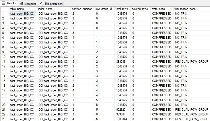
The results provide a bit more information about rowgroups and their contents:

Note that the row group IDs are repeated as they are spread across 5 partitions. The combination of row_group_id and partition_number will be unique within a given columnstore index that has table partitioning enabled.

This index is close to optimal, with most rowgroups full or nearly full. The data above indicates to an operator that no index maintenance is needed at this time. The trim reason tells us why a rowgroup was closed before being filled to the maximum allowed size.

We can add some churn into the index for use in the further demo below:

UPDATE fact_order_BIG_CCI
        SET Quantity = 1
FROM dbo.fact_order_BIG_CCI
WHERE fact_order_BIG_CCI.[Order Key] >= 8000101
AND fact_order_BIG_CCI.[Order Key] < 8001001;
GO
DELETE fact_order_BIG_CCI
FROM dbo.fact_order_BIG_CCI
WHERE fact_order_BIG_CCI.[Order Key] >= 80002001
AND fact_order_BIG_CCI.[Order Key] < 80002501;
GO
INSERT INTO dbo.fact_order_BIG_CCI
SELECT TOP 1 * FROM dbo.fact_order_BIG_CCI
GO 100

As a reminder, these types of small write operations are not optimal for a columnstore index. Rerunning the query against sys.dm_db_column_store_row_group_physical_stats reveals some changes. Filtering by state_desc and deleted_rows reduces the rows returned, which is especially useful against a large columnstore index:

SELECT
    tables.name AS table_name,
    indexes.name AS index_name,
    partitions.partition_number,
    dm_db_column_store_row_group_physical_stats.row_group_id,
    dm_db_column_store_row_group_physical_stats.total_rows,
    dm_db_column_store_row_group_physical_stats.deleted_rows,
    dm_db_column_store_row_group_physical_stats.state_desc,
    dm_db_column_store_row_group_physical_stats.trim_reason_desc
FROM sys.dm_db_column_store_row_group_physical_stats
INNER JOIN sys.indexes
ON indexes.index_id = 
    dm_db_column_store_row_group_physical_stats.index_id
AND indexes.object_id = 
    dm_db_column_store_row_group_physical_stats.object_id
INNER JOIN sys.tables
ON tables.object_id = indexes.object_id
INNER JOIN sys.partitions
ON partitions.partition_number = 
    dm_db_column_store_row_group_physical_stats.partition_number
AND partitions.index_id = indexes.index_id
AND partitions.object_id = tables.object_id
WHERE tables.name = 'fact_order_BIG_CCI'
AND (dm_db_column_store_row_group_physical_stats.state_desc 
    <> 'COMPRESSED'
OR   dm_db_column_store_row_group_physical_stats.deleted_rows > 0)
ORDER BY indexes.index_id, 
    dm_db_column_store_row_group_physical_stats.row_group_id;

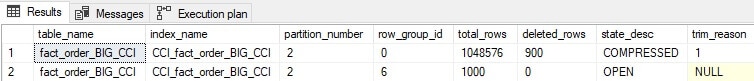
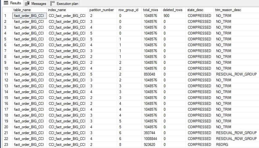
The results are as follows:

An existing rowgroup has been updated to show that it contains 900 deleted rows. These rows will remain in the columnstore index until rebuilt. A new deltastore has been created to store the 1000 rows that were recently inserted. It is open, indicating that more rows can be added as needed. This allows the 1000 insert operations executed above to be combined into a single rowgroup, rather than lots of smaller ones.

Reorganize

A clustered columnstore index may be reorganized as an online operation. As such, this maintenance can be performed anytime without blocking access to it. This operation will take whatever is in the deltastore and process it immediately, as though the tuple mover was running and handling it.

The primary benefit of reorganizing a columnstore index is to speed up OLAP queries by removing the deltastore rowstore records and moving them to the columnstore index structure. Queries no longer need to read data from the deltastore to get the data they need. In addition, since the index is highly compressed, the memory required to read the data needed to satisfy a query is smaller.

The syntax to reorganize a columnstore index is similar to that for a standard B-tree index:

ALTER INDEX CCI_fact_order_BIG_CCI ON dbo.fact_order_BIG_CCI REORGANIZE;

Reviewing the physical stats for this index shows the following results:

No changes! The reason that there is still an open rowgroup is that SQL Server is waiting for more rows to be added before compressing and adding it to the columnstore index. Having a large volume of tiny rowgroups would be inefficient as the ideal size is 220 rows, and the closer we can get to that magic number, the better.

We can force the tuple mover to process the deltastore, close it, and commit it to compressed data within the columnstore index by using the following variant on the reorganize statement:

ALTER INDEX CCI_fact_order_BIG_CCI ON dbo.fact_order_BIG_CCI 
REORGANIZE WITH (COMPRESS_ALL_ROW_GROUPS = ON);

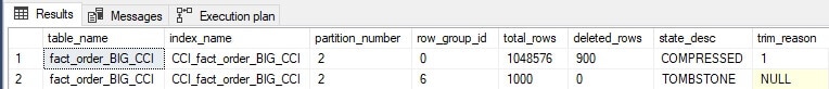
The results look like this:

A rowgroup that is labelled with the state TOMBSTONE indicates that it was a part of a deltastore and was forcefully compressed into a columnstore rowgroup. The residual rowgroup no longer has any non-deleted rows in it and therefore is labelled with the ominous tombstone state. These are intermediary rowgroups that will be deallocated. We can force this along with another reorganization command, and the tombstone rowgroup is gone.

Note that there is no need to force this change. Doing so demonstrates how automated processes can be started to fast-track a given result. Given time, this cleanup will occur anyway. Therefore there is no compelling reason to do this in a production environment.

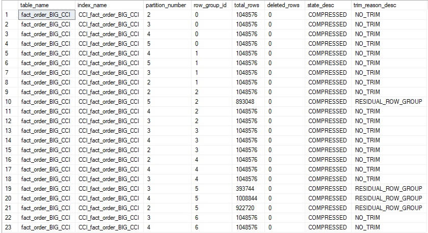
The final version of the columnstore index can be viewed by removing the filters on state_desc and deleted_rows:

There are 23 compressed rowgroups, and the trim reason for the final rowgroup has been changed to REORG, indicating that it was opened and closed via an index reorganization process. Note that the index has the same number of rowgroups as earlier and row counts that are more than acceptable for OLAP operations.

Rebuild

Rebuilding a clustered columnstore index is an offline operation until SQL Server 2019 when the ability to rebuild online was introduced. As with a B-tree index, the rebuild will create a brand new columnstore index from the underlying data. Doing so will:

  1. Eliminate all data in the deltastore.
  2. Eliminate all deleted rows.
  3. Reduce the number of compressed rowgroups, if large numbers of smaller ones exist.

This operation is expensive and should be reserved for a dedicated maintenance window and only when the index has become so fragmented that no other options exist.

Note that the order of data is not changed when the columnstore index is rebuilt. Similar to when our demo table was first created, if no order is enforced, then SQL Server will build a new index on top of our data as-is. If the columnstore index table has been maintained by adding data in order over time, then odds are good that no special work will be needed to re-order it.

The columnstore index we have been tinkering with thus far can be rebuilt like this:

ALTER INDEX CCI_fact_order_BIG_CCI ON dbo.fact_order_BIG_CCI 
REBUILD WITH (ONLINE = ON);

Note again that the ONLINE option is not available prior to SQL Server 2019. For this table, the rebuild takes about 2 minutes. Reviewing all rowgroups in the table reveals the following:

The deleted rows are gone, and rows from other rowgroups were pushed into the vacancy left behind. While there are still some rowgroups that are not completely full, this index is quite efficiently structured overall.

If table partitioning is in use, then index rebuilds become significantly less expensive as the active partition(s) can be targeted for a rebuild and the rest ignored. In a table where a large portion of the data is old and unchanged, this can save immense system resources, not to mention time!

The syntax to rebuild a specific partition is as follows:

ALTER INDEX CCI_fact_order_BIG_CCI ON dbo.fact_order_BIG_CCI 
REBUILD PARTITION = 5
WITH (ONLINE = ON);

When executed, the rebuild will only target partition 5. If this is the active partition and the others contain older static data, then this will be the only partition with fragmentation, assuming no unusual change has occurred on older data. The rebuild of partition 5 shown above took about 20 seconds to complete.

The simplest way to measure when a columnstore index needs a rebuild is to measure the quantity of deleted rows and compare it to the total rows for each partition. If a partition contains 1 million rows of which none are deleted, then it’s in great shape! If a partition contains 1 million rows, of which 200k are flagged for deletion, then a rebuild would be a good idea to remove those soft-deleted rows from the index.

The following query groups columnstore index metadata by table, index, and partition, allowing for a relatively simple, but useful view of fragmentation:

SELECT
    tables.name AS table_name,
    indexes.name AS index_name,
    partitions.partition_number,
    SUM(dm_db_column_store_row_group_physical_stats.total_rows) 
        AS total_rows,
    SUM(dm_db_column_store_row_group_physical_stats.deleted_rows) 
        AS deleted_rows
FROM sys.dm_db_column_store_row_group_physical_stats
INNER JOIN sys.indexes
ON indexes.index_id = 
    dm_db_column_store_row_group_physical_stats.index_id
AND indexes.object_id = 
    dm_db_column_store_row_group_physical_stats.object_id
INNER JOIN sys.tables
ON tables.object_id = indexes.object_id
INNER JOIN sys.partitions
ON partitions.partition_number = 
    dm_db_column_store_row_group_physical_stats.partition_number
AND partitions.index_id = indexes.index_id
AND partitions.object_id = tables.object_id
WHERE tables.name = 'fact_order_BIG_CCI'
GROUP BY tables.name, indexes.name, partitions.partition_number

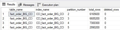
The results of this query are as follows:

This specific example provides insight into an index that requires no maintenance. If the count of deleted rows was high enough, though, then a rebuild of that partition could save storage, memory, and make queries against that data faster. Note that deleted_rows includes both rows that were deleted and those that were updated, since an update is modelled as a delete followed by an insert.

Additional Index Maintenance Notes

In general, a common plan for index maintenance is as follows:

  1. Perform an index reorganization with the compress_all_row_groups option on after any large data load, or on a semi-regular basis. This is inexpensive, online, and will generally keep an index defragmented enough for efficient use for quite a long time.
  2. Perform infrequent index rebuilds on heavily fragmented partitions (if partitioned) or the entire index (if not). Perform this online, if available, as it will eliminate the need for either a maintenance window or data trickery to avoid a maintenance window.

If a columnstore index is loaded solely via inserts (no deletes or updates) and the data is consistently inserted in order, then fragmentation will occur very slowly over time, and index rebuilds will be rarely (if ever) needed.

OLAP databases are uniquely positioned to take advantage of this fact, as their data loads are typically isolated, primarily inserts, and performed at designated intervals. This differs from OLTP databases, that are often the target of deletes, updates, software releases, and other operations that can quickly cause heavy fragmentation.

Nonclustered Columnstore Indexes

The discussion of columnstore indexes thus far has focused on clustered columnstore indexes that target a primarily OLAP workload. SQL Server also supports nonclustered columnstore indexes. A table may only have one columnstore index on it at a time, regardless of whether it is clustered or nonclustered. A nonclustered columnstore index functions similarly to a clustered columnstore index in terms of architecture, data management, the deltastore, and other nuances discussed thus far in this article.

To illustrate the effects of a nonclustered columnstore index, consider the following query:

SELECT
        SUM([Quantity])
FROM dbo.fact_order_BIG
WHERE [Order Date Key] >= '1/1/2016'
AND [Order Date Key] < '2/1/2016';

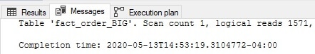
This is executing against a table without a columnstore index, but with a nonclustered index on [Order Date Key]. When executed, there is a bit of waiting, and the result is returned. The following is the IO for the query:

That sort of IO is not acceptable against a busy OLTP table and will cause latency and contention for other users that are reading and writing data to this table. If this is a common query, then a nonclustered columnstore index can address it:

CREATE NONCLUSTERED COLUMNSTORE INDEX NCI_fact_order_BIG_Quantity 
ON dbo.fact_order_BIG ([Order Date Key], Quantity);

By choosing only the columns needed to satisfy the query, the need to maintain a larger and more expensive structure on top of an OLTP data store is avoided. Once complete, the IO for the test query above is significantly reduced:

Note that while IO is 1/10th of the previous cost and the query executed much faster, IO is still high and the details above indicate that no segments were skipped.

Similar to the clustered columnstore index, data order bit us here. If the underlying table were ordered primarily by [Order Date Key], then segments could be skipped as part of query execution. Without that implicit ordering, the efficiency of a nonclustered columnstore index is hindered far more than it would have been if a clustered columnstore index were used.

This poses a challenge to a database architect: Is placing a nonclustered columnstore index on top of an OLTP workload worth the effort? Would a covering index be better? This question can be tested:

DROP INDEX NCI_fact_order_BIG_Quantity ON dbo.fact_order_BIG;
CREATE NONCLUSTERED INDEX NCI_fact_order_BIG_Quantity 
ON dbo.fact_order_BIG ([Order Date Key]) INCLUDE (Quantity);

The new index sorts on [Order Date Key] and adds Quantity as an include column. The following is the IO after this change

A covering nonclustered B-tree index provided more efficient coverage of this query than the nonclustered columnstore index.

Ultimately, the challenge presented here is to separate OLAP and OLTP workloads. Even if a nonclustered columnstore index can be built that is well-ordered and satisfies a query efficiently, it will become fragmented quickly if write operations target the table with frequent inserts, updates, and deletes. The best possible solution to this problem is to separate heavy OLAP workloads from OLTP into their own databases and tables.

The test query above filtered a single column and returned one other. Typically, the hole that administrators and developers fall into with OLAP against OLTP is that it is never just one column. Once reporting against OLTP data ensues, there often ends up being many analytics against many columns that result in the creation of many covering indexes to handle each scenario. Eventually, an OLTP table becomes overburdened by covering indexes and hefty reporting queries that cause contention against critical OLTP workloads.

While nonclustered columnstore indexes exist and can provide targeted relief for expensive OLAP queries, they require heavy testing prior to implementing to ensure that they are efficient, ordered, and can outperform a classic covering index. It is also necessary to ensure that an OLTP database does not become overburdened with OLAP workloads over time.

This is a significant challenge that many administrators and developers struggle with regularly. Ultimately, if reporting data and queries can be separated into their own data store, then we can properly implement a clustered columnstore index. Data can then be architected and ordered to optimize solely for OLAP workloads without the need to be concerned for the impact of those analytics against other real-time transactions.

Memory-Optimized Columnstore Indexes

Because columnstore indexes are compact structures, the ability to natively store them in-memory becomes possible. The example table in this article was 5GB when stored via a classic B-tree clustered index. While not massive, this is also not trivial. If the table were to grow by 5GB every year, then reading the entire thing into memory may not be worth it. Alternatively, the 100MB used for the columnstore index is trivial with regards to memory consumption.

If reporting against a columnstore index requires speed, then converting it into a memory-optimized table is an option for potentially improving performance. Note that data compression in-memory is not as efficient as on disk. As a result, results may vary depending on available memory. Typically, memory-optimized data size will be at least double the size of a disk-based columnstore index.

On a server with limited memory, this will pose a challenge, and testing will be necessary to determine if this is a worthwhile implementation of memory-optimized tables or not. The following is the basic T-SQL syntax needed to create a new memory-optimized columnstore index table:

CREATE TABLE dbo.fact_order_BIG_CCI_MEM_OPT (
    [Order Key] [bigint] NOT NULL 
        CONSTRAINT PK_fact_order_BIG_CCI_MEM_OPT 
        PRIMARY KEY NONCLUSTERED HASH WITH (BUCKET_COUNT = 100000),
    [City Key] [int] NOT NULL,
    [Customer Key] [int] NOT NULL,
    [Stock Item Key] [int] NOT NULL,
    [Order Date Key] [date] NOT NULL,
    [Picked Date Key] [date] NULL,
    [Salesperson Key] [int] NOT NULL,
    [Picker Key] [int] NULL,
    [WWI Order ID] [int] NOT NULL,
    [WWI Backorder ID] [int] NULL,
    [Description] [nvarchar](100) NOT NULL,
    [Package] [nvarchar](50) NOT NULL,
    [Quantity] [int] NOT NULL,
    [Unit Price] [decimal](18, 2) NOT NULL,
    [Tax Rate] [decimal](18, 3) NOT NULL,
    [Total Excluding Tax] [decimal](18, 2) NOT NULL,
    [Tax Amount] [decimal](18, 2) NOT NULL,
    [Total Including Tax] [decimal](18, 2) NOT NULL,
    [Lineage Key] [int] NOT NULL,
INDEX CCI_fact_order_BIG_CCI_MEM_OPT CLUSTERED COLUMNSTORE)
WITH (MEMORY_OPTIMIZED = ON, DURABILITY = SCHEMA_AND_DATA);

Note that a primary key is required on all memory-optimized tables. Now, this table can be loaded with test data:

INSERT INTO dbo.fact_order_BIG_CCI_MEM_OPT
SELECT
    [Order Key] + (250000 * ([Day Number] + 
        ([Calendar Month Number] * 31))) AS [Order Key]
    ,[City Key]
    ,[Customer Key]
    ,[Stock Item Key]
    ,[Order Date Key]
    ,[Picked Date Key]
    ,[Salesperson Key]
    ,[Picker Key]
    ,[WWI Order ID]
    ,[WWI Backorder ID]
    ,[Description]
    ,[Package]
    ,[Quantity]
    ,[Unit Price]
    ,[Tax Rate]
    ,[Total Excluding Tax]
    ,[Tax Amount]
    ,[Total Including Tax]
    ,[Lineage Key]
FROM Fact.[Order]
CROSS JOIN
Dimension.Date
WHERE Date.Date <= '2013-04-10';

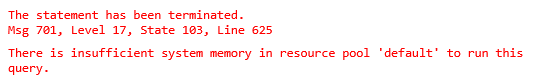
This insert executes for about ten seconds on my local server and throws the following error:

Ouch! Reducing the date range should allow for a test data set to be created without running my server out of memory. To do this, ‘2013-04-10’ will be replaced with ‘2013-02-01’. The result is a table that can be queried like before using a test query:

SELECT
        SUM([Quantity])
FROM dbo.fact_order_BIG_CCI_MEM_OPT
WHERE [Order Date Key] >= '2016-01-01'
AND [Order Date Key] < '2016-02-01';

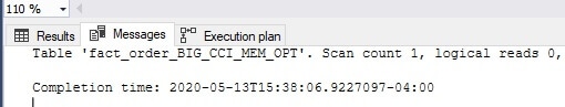
The results are returned with zero IO:

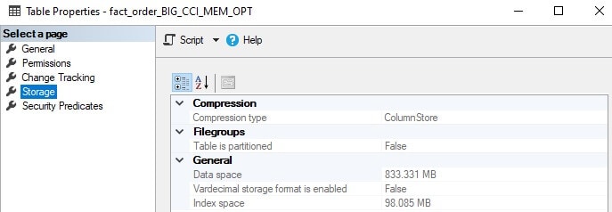
As expected, querying a table that resides in memory results in zero reads. Despite that, it still takes time to read data from memory, and therefore this is not a freebie! Here is the storage footprint for the table:

Another Ouch! More space is consumed for 15 days of data than for the entire clustered columnstore index implemented on disk earlier. While additional optimization is possible, the overhead for maintaining the primary key on the data is not cheap, and it is hard to justify this cost unless there will be other uses for the memory-optimized data as well.

Because a columnstore index is relatively small to start with, much of it can fit into the buffer cache and be available in memory to service queries against it. The memory-optimized columnstore index will need to outperform its counterpart when in the cache, which is possible, but less impressive.

While this can trigger a lengthy discussion of memory-optimized objects, we are better served by avoiding it as the benefits will be limited to highly niche cases that are out of the scope of a general columnstore index dive.

When considering a memory-optimized columnstore index, the following will assist in making a decision:

  1. Is speed currently acceptable? If so, do not put into memory.
  2. Is extra memory available for the table, if a memory-optimized option is chosen?
  3. Can the active partition be segregated and placed in memory and the rest of a table on disk?
  4. Can the table benefit from SCHEMA_ONLY durability? I.e., is the table disposable if the server is restarted?
  5. Can testing validate that a memory-optimized table will perform significantly better?

Memory-optimized tables were built by Microsoft to specifically address the problem of highly concurrent OLTP workloads. One of the greatest selling points of memory-optimized tables is the elimination of locking, latching, and deadlocks. These should rarely be concerns for large OLAP workloads. With this in mind, putting a columnstore index into memory will rarely be worth the effort. In some special cases, it will provide speed boosts, but significant testing is needed to confirm this.

In addition, all of the various limitations imposed on memory-optimized objects apply here, which may also sway one’s opinion to use them. This page provides up-to-date details on what features are supported or not for memory-optimized tables:

Conclusion

The more I explored columnstore indexes, the more I appreciated them. Many of the optimizations and tweaks that can allow for OLAP data loads to be processed even faster are not well documented. Still, they can significantly improve the speed of data loads, archiving processes, and reporting. This is a feature that will continue to grow in popularity as data continues to grow and will add value to any organization that wants to maintain control over their reporting data.

There is no room here for “set it and forget it”. Implementing columnstore indexes should be treated with the same level of care as architecting new OLTP tables. The results will perform well, even for massive quantities of data. In addition, maintenance, upgrades, and software releases will be faster, easier, and less risky.

Columnstore is one of my favorite features in SQL Server. It has revitalized how OLAP data is stored and accessed, allowing for billions of rows of data to be efficiently stored and quickly accessed in ways that previously were challenging to achieve without moving data into other analytics tools. The biggest bonus of retaining OLAP data in SQL Server is that we (the developers, administrators, and analysts) can keep control over analytic data architecture and ensure optimal performance as organizational and software changes continually happen.

The post Hands-On with Columnstore Indexes: Part 3 Maintenance and Additional Options appeared first on Simple Talk.


from Simple Talk https://ift.tt/2WGTJxz
via