Understanding how to join the data in one table to another is crucial for any data analyst or database developer working with a relational database. Whether you’re a beginner or an experienced SQL user, this article will help you strengthen your SQL skills and become proficient in SQL joins.
With several types of joins available, it can be overwhelming to understand the differences and choose the right one for your query. Each join type is very similar, but different in a few very important ways. In this article, we’ll explore various types of SQL joins using PostgreSQL (though a lot of this will work in most other RDBMSs out there).
There are multiple types of joins that go by very similar names including inner joins, left outer joins, right outer joins, full outer joins, and cross joins. We will cover all these types, as well as a few join subtypes of joins, including self and natural joins. We’ll explain their functionalities and use cases and provide examples to help you grasp the concepts more effectively.
Prerequisites
To get started with the material in this article, the following will be very helpful.
- Knowledge of SQL basic
- Familiarity with SQL tables and their structures.
Note that if you are a novice with PostgreSQL (or any other RDBMS, most of this should be relatively straightforward.) In addition, the following skills will be helpful:
- Basic knowledge of SQL syntax and structure will be helpful.
- Familiarity with PostgreSQL or similar SQL database management system
- Access to a PostgreSQL database for practicing SQL queries. How to install PostgreSQL will be covered early in the article.
Setting up the database environment
In this article, we will explore the different types of SQL joins and explain how to use them effectively using PostgreSQL. By the end of this article, you will clearly understand each join type and when to use it. If you want to follow along and try out the concepts presented, there are a few things we need to set up; including the database server, the tools, and a database to query.
Installing PostgreSQL cluster
To follow along, you will need access to a database environment. To set up a PostgreSQL database environment, visit www.postgresql.org, choose the appropriate version for your OS, and follow the installation instructions. Download both the server and its components. The article was written using Postgres 15 as the platform, but during the editorial process, PostgreSQL 16 was released. All of the code will execute on PostgreSQL 16 and other recent versions of PostgreSQL.
For accurate and detailed instructions about the different releases of PostgreSQL, refer to the official documentation on their website. It will provide comprehensive resources for setup and usage.
Installing pgAdmin
Additionally, we will leverage pgAdmin, a robust graphical interface that streamlines the creation, maintenance, and utilization of database objects. It caters to the requirements of both novice and seasoned Postgres users. Follow the download instruction and documentation to set up properly. (Note that pgAdmin may be able to be installed with your RDBMS install.)
Installing the Sample Database
To give us tables and data to join, we will use a sample relational database called Northwind. The Northwind database is a well-known and widely used sample database in database management. Created by Microsoft, it serves as a popular tool for demonstrating concepts in database courses, tutorials, and examples. The Northwind database depicts a fictional company known as “Northwind Traders,” which sells various products to customers. It consists of multiple tables representing the company’s operations, including customers, orders, products, suppliers, employees, and categories. These tables are interconnected through relationships, facilitating complex queries and data analysis.
To install Northwind, follow the instructions on Wikiversity. The process straightforward and includes a script that creates the tables and data without even needing to restore a database. The following diagram is the Entity-Relationship (ER) diagram that shows the tables, columns, and relationships between the tables in the database. As we write some of the code, it can be helpful to see own tables are related to one another.
Note: in the diagram, the lines between the tables show a relationship between the tables. The solid dot is the table that is the child in the relationship. The other table is the parent, and its primary key (the column that is in bold above the line in each table that is the primary way to identify a row in a table) from the parent is repeated in the child table to form the connection we will use in sample queries.
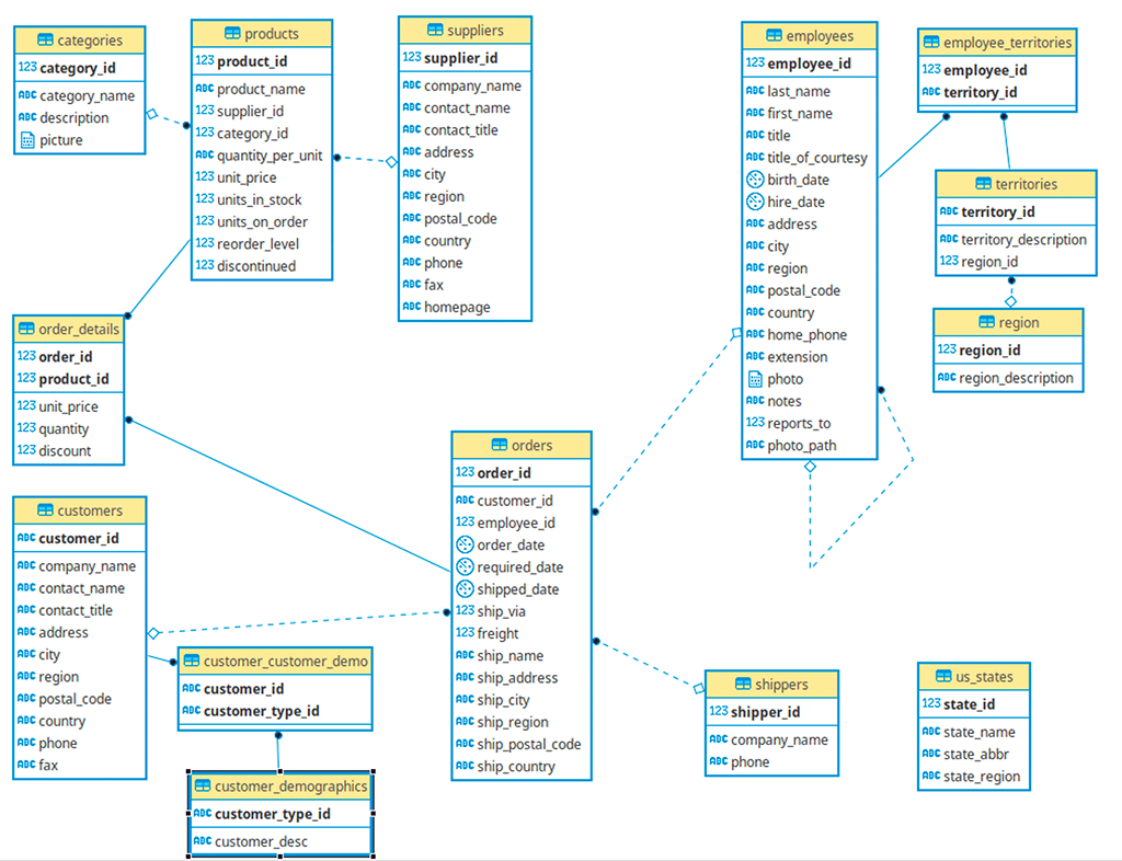
Northwind Database Schema
General Join Principles
Understanding the syntax, process, and various join types is crucial for harnessing the full potential of database management systems and allow you to combine data in very interesting ways. In this section, we will delve into joins, exploring their general syntax, the underlying process, handling matching and non-matching rows, and the differences in join types.
A join in a relational database typically involves using SQL to specify the tables to be joined, the join condition, and the desired columns in the result set.
The Process of Joining Tables:
The process of joining tables entails the following steps:
- Identifying the Tables: Determine the tables you want to join based on the data you need to combine and the relationships between them.
- Identifying the Join Condition: Identify the column(s) in the tables that have matching values and will serve as the join condition.
- Choosing the Join Type: Select the appropriate join type based on the desired output, such as an inner join, left join, right join, or full outer join.
- Writing the Joins: Compose the SQL query using the chosen join type and the specified join condition.
- Executing the Query: Execute the query against the database and retrieve the joined result set.
When joining tables, some rows will have matching values in the specified join condition, while others will not. What happens to the different values will be based on the type of join you use.:
- Matched Rows: Rows with matching values in the join condition will be included in the joined result set. The columns from both tables will be combined based on the join condition.
- Non-Matched Rows: Rows that do not have matching values in the join condition will be handled differently based on the join type.
As an example, say you have two tables X and Y. We will use these tables for some simple example queries before moving to the Northwind tables.
CREATE TABLE X (
Xid int CONSTRAINT PKX PRIMARY KEY
);
CREATE TABLE Y (
Yid int CONSTRAINT PKY PRIMARY KEY,
Xid int --should be an FK constraint
--but left off for examples.
);

INSERT INTO X (Xid)
VALUES (1),(2),(3);

INSERT INTO Y (Yid, Xid)
VALUES (1,2),(2,3),(3,3),(4,4);
After creating the tables and executing the INSERT statements, the tables have the following data.
Table X:
Table Y:
Since table Y references table X (commonly referred to as being a child of table X), we need to connect the data using the value in the Y table that references the data in table X.
Putting the tables side by side, matching on the Xid column using the join criteria is X.Xid = Y.Xid, we can see how the data matches:.
| X.Xid |
Y.Yid |
Y.Xid |
| 1 |
|
|
| 2 |
1 |
2 |
| 3 |
2 |
3 |
| 3 |
3 |
3 |
| |
|
4 |
Note that for Xid = 3, two Y rows match one X row, so that data has been duplicated. The queries we will write will connect the two tables in variations of this pattern.
Join Styles
You can specify join criteria in the WHERE or FROM clause of a statement. Although both approaches can produce the same results in certain situations, they differ in functionality and recommended usage.
- Explicit Join: Using the
JOIN keyword to connect objects to join, you specify the join join criteria in an ON clause. This is known as explicit join notation, which involves using the ON keyword to specify the predicates or conditions for the join and the JOIN keyword to indicate the tables to be joined.
This approach explicitly defines how the tables relate, improving query readability and organization. For more complex queries, evaluating the join conditions early can allow the database engine to optimize the query execution plan, potentially leading to enhanced performance.
Syntax:
SELECT column_names
FROM Table1
    JOIN Table2
     ON Table1.column_name = Table2.column_name
- Implicit Join: In this notation, the tables to be joined are listed in the
FROM clause of the SELECT statement, separated by commas. The join predicates are then specified in the WHERE clause. This method has limitations; it does not support OUTER joins naturally. If one is not cautious, it can easily produce results equivalent to a CROSS join, especially when the join criteria are missed or mistaken. it can result in less readable and less optimized queries, particularly when working with large datasets or complex joins.
Syntax:
SELECT column_names
FROM   Table1, Table2
WHERE  Table1.column_name = Table2.column_name
Relationships
Next, let’s explore SQL relationships essential for comprehending joins. Joins allow us to merge data from multiple tables based on their relationships. Relationships play a pivotal role in organizing and connecting data between different tables.
Relationships allow you to facilitate normalization, as they enable you to store related information in separate tables and eliminate duplicated data. Joins will allow you to re-combine the data as needed during queries for usage.
They essentially define how data in one table is related to data in another table. The three fundamental types of relationships are one-to-one, one-to-many, and many-to-many. In the diagram, the end with the “crow’s foot” represents the relationship where one or more rows can be related:
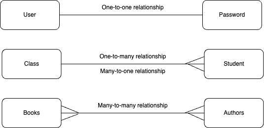
Source: Author
- One-to-One Relationship: In relational database design, a one-to-one (1:1) relationship signifies that a record in Table A is associated with zero or one record in Table B (note that one table will need to be considered the parent in the relationship due to how relationships are implemented.). In this relationship, each record in Table A corresponds to a single record in Table B, and no duplicate values are allowed. One-to-one relationships are typically used when data needs to be separated into multiple tables for normalization or security purposes.
- One-to-Many Relationship: In relational database design, a one-to-many (1:N) relationship signifies that one instance of Table A can be associated with zero, one, or more instances of Table B. In comparison, each instance of Table B can relate to zero or one instance of Table A. One-to-many relationships are widely used to represent hierarchical or parent-child relationships between data.
- Many-to-Many Relationship: In relational database design, a many-to-many (M:N) relationship means multiple records in Table A can associate with multiple records in Table B and vice versa. Specifically, an instance from Table A can relate to zero, one, or more instances of Table B, and similarly, an instance from Table B can link to zero, one, or more instances of Table A.
When working with joins, it’s essential to understand the relationships that the designer intended between the tables you are joining thoroughly. This includes recognizing both matching and non-matching rows or instances between the tables. The presence or absence of multiple matches can influence the outcome of the join operation. Being attentive to these details ensures accurate interpretation of the results and maintains data integrity.”
SQL join types play a crucial role in determining the treatment of matching and non-matching rows during the join operation. Let’s explore a concise summary of the distinctions between various join types.
Join Type Overview
In this section I will go describe each of the join types, and then in the next section we will work through some examples.
Inner Join
An inner join returns only the rows with matching values in the specified column(s) from both tables. It combines data from two tables based on the common column(s) and eliminates non-matching rows.
Syntax:
SELECT *
FROM X
INNER JOIN Y
ON X.Xid = Y.Xid;
Using the tables we created earlier. This query will return:
| xid |
yid |
xid |
| 2 |
1 |
2 |
| 3 |
2 |
3 |
| 3 |
3 |
3 |
Looking at the columns, they will be based on the table to the left of the join first, then the tables from the right column. Note that xid = 1 does not show up in the results for the X table and xid = 4 does not show up from the Y table..
Left Outer Join:
Left outer join returns all rows from the left table (Table1) and the matching rows from the right table (Table2). Non-matching rows in the right table will contain NULL values in the result set.
Syntax:
SELECT *
FROM X
LEFT JOIN Y
ON X.Xid = Y.Xid
Now the results are the same, except there is one additional row returned. The X row where xid = 1 will show up now with NULL values for all of the values for the Y table’s columns.
| xid |
yid |
xid |
| 2 |
1 |
2 |
| 3 |
2 |
3 |
| 3 |
3 |
3 |
| 1 |
|
|
Right Outer Join
Right outer join returns all rows from the right table (Table2) and the matching rows from the left table (Table1). Non-matching rows in the left table will contain NULL values in the result set. If you change the join to be a RIGHT JOIN:
SELECT *
FROM X
RIGHT JOIN Y
ON X.Xid = Y.Xid;
The output now includes the Y row where xid = 4.
| xid |
yid |
xid |
| 2 |
1 |
2 |
| 3 |
2 |
3 |
| 3 |
3 |
3 |
| |
4 |
4 |
Full Outer Join:
Full outer join returns all rows from both tables, including matching and non-matching rows.
Syntax:
SELECT *
FROM X
FULL OUTER JOIN T
ON X.Xid = Y.Xid;
Now you will see we are back to the version of the output that was shown when I showed you the data side by side.
| xid |
yid |
xid |
| 2 |
1 |
2 |
| 3 |
2 |
3 |
| 3 |
3 |
3 |
| 1 |
|
|
| |
4 |
4 |
This is very often used to find rows in two tables where some condition is not true in two tables. Like in this case I can find all rows where X.Xid is not in Y and Y.Xid is not in X by adding where X.Xid is null or Y.Xid is null. Then your output will be just he last two rows.
Cross Join:
Cross join (also known as Cartesian join) returns the Cartesian product of both tables. It combines each row from the first table with every row from the second table, resulting in a potentially large result set. One of the more common uses of the CROSS JOIN is to add the contents of a single row to a lot of rows. Note that there is no join criteria, and every row in one input matches every row in the other.
Syntax:
SELECT *
FROM X
CROSS JOIN Y;
The output of this query a lot longer than the others, because it will return (number of rows in X) * (number of rows in Y) rows. In this case 3 * 4 or 12 rows.
| xid |
yid |
xid |
| 1 |
1 |
2 |
| 1 |
2 |
3 |
| 1 |
3 |
3 |
| 1 |
4 |
4 |
| 2 |
1 |
2 |
| 2 |
2 |
3 |
| 2 |
3 |
3 |
| 2 |
4 |
4 |
| 3 |
1 |
2 |
| 3 |
2 |
3 |
| 3 |
3 |
3 |
| 3 |
4 |
4 |
Note too that the following will output the same results:
SELECT *
FROM X,Y;
And this too, because just like the CROSS JOIN, every row matches every other row.:
SELECT *
FROM Y
INNER JOIN X
      ON 1=1; --any criteria that is always true
Join Subtypes
The following examples are syntaxes but are types of joins you can do that are interesting to understand.
Self Join
A self join involves joining a table to itself, treating it as two separate instances. It allows for comparing and combining rows within the same table based on specified column(s).
Syntax:
SELECT *
FROM X
INNER JOIN X AS T2
ON X.Xid = T2.Xid;
Note that if the column used is the PRIMARY KEY, it will basically just duplicate all of the data in Table1 twice (as you would see if you executed the sample query). This type of query is typically done with things like employee and manager relationships.
For example, if Table1 was Employee, with an EmployeeId for the primary key value, you might have a column ManagerEmployeeIdand you would execute:
SELECT *
FROM Employee
INNER JOIN Employee AS Manager
   ON Employee.ManagerEmployeeId = Manager.EmployeeId
Natural Join
A natural join automatically matches columns with the same name in the two tables being joined. It eliminates the need to specify the join condition explicitly, assuming that column names and datatypes match accurately.
SELECT *
FROM X
NATURAL JOIN Y;
The output from this query will be just like the INNER JOIN example except for one thing. The column that is used for the join criteria (or criterion if you have multiple columns with the same name) will not be repeated. So the output will be:
Note that in the example above, that is an INNER join on the columns that match in X and Y. You can do a NATURAL OUTER JOIN, or any of the other join types as well, the NATURAL modifier just makes it use the columns from the tables.
Join Examples
Mastering the art of joining tables is a fundamental skill for anyone working with relational databases. By understanding the general syntax, the underlying process, and the differences in join types, you can effectively combine data from multiple tables, extract meaningful insights, and unleash the power of your database management system. With this knowledge, you’ll be well-equipped to navigate the world of generic joins and leverage their capabilities to your advantage.
In this section, we will go through some examples using the Northwind database that we included instructions for early in the article.
Inner Join
Let’s examine what a few tables look like that we are going to be joining together for an INNER JOIN. First, the customer table looks like by returning a few rows from the table. Using pgAdmin, start a new query in the Northwind database and execute the following query:
SELECT *
FROM customers
LIMIT 5;
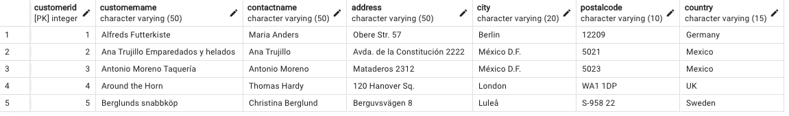
Query results from PgAdmin, Source Author
This returns 5 rows from the table. For small databases on limited servers, this will almost always return the same data, but be aware that without an ORDER BY clause, there is no guarantee of any order to the output.
Next, let us quickly examine the orders table that we intend to join with the customers table.
SELECT *
FROM orders
LIMIT 5;
This query will retrieve 5 rows from the orders table and display all columns for each of those rows.
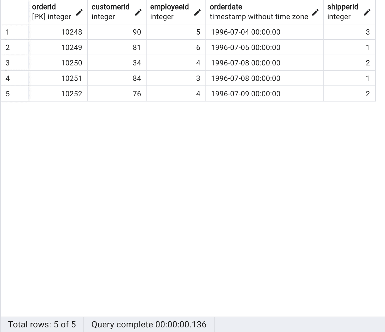
Query results from PgAdmin, Source Author
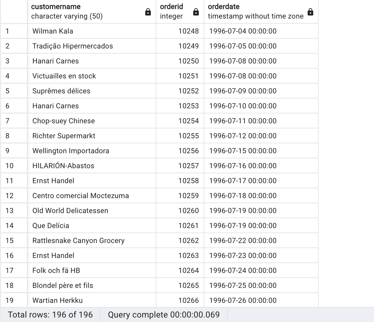
We will now perform an INNER JOIN between the orders table and the customers table, resulting in the following query:
SELECT c.customername, o.orderid, o.orderdate
FROM customers c
      INNER JOIN orders o
         ON c.customerid = o.customerid
LIMIT 5;
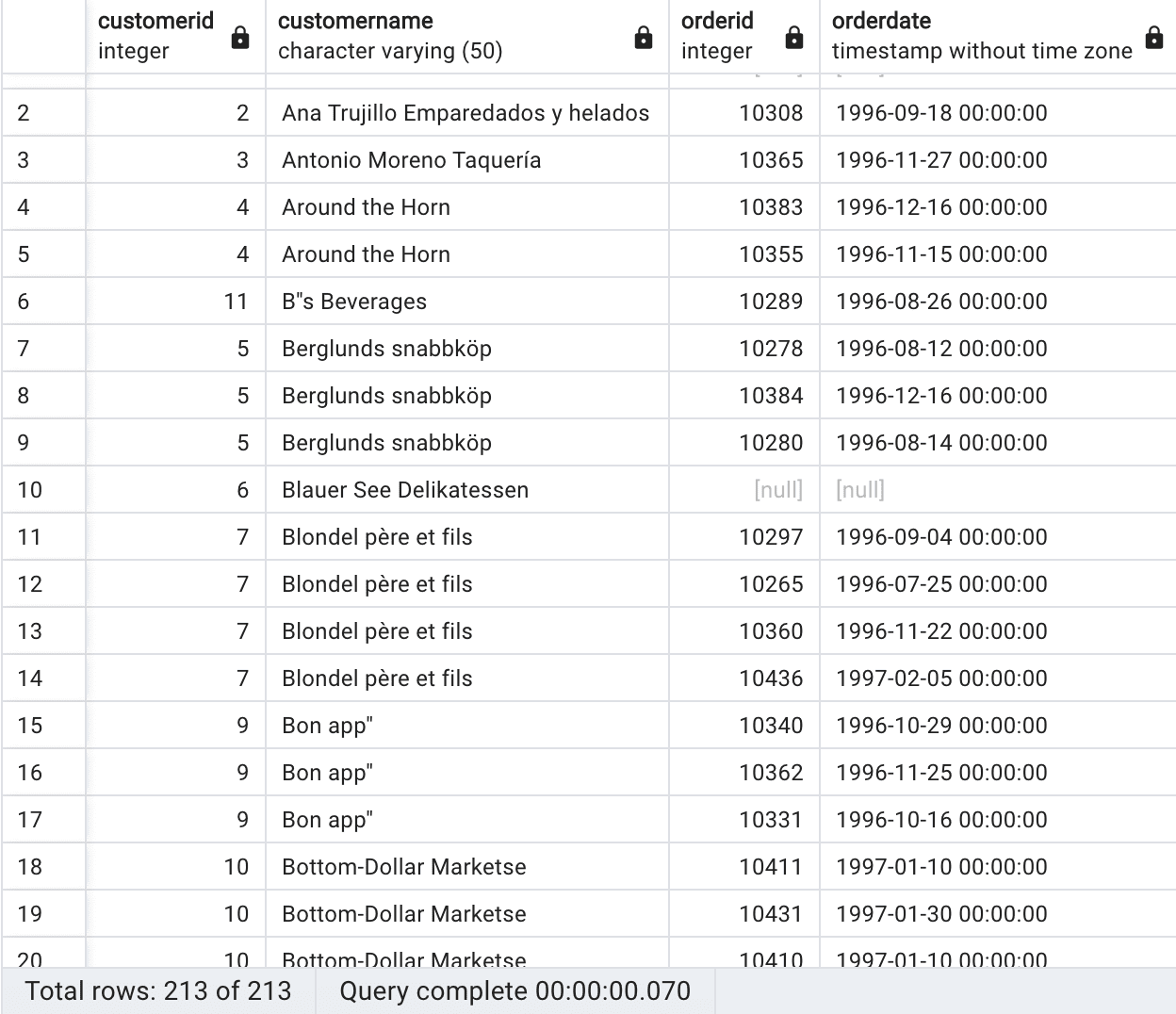
This query will retrieve a result set of five rows (the LIMIT clause will cut off the output of rows at the number specified) that includes the customer’s name, order ID, and order date for all customer orders in the Customers table. Using an INNER JOIN, only rows with matching customer IDs in the customer and orders tables will be included in the result set.
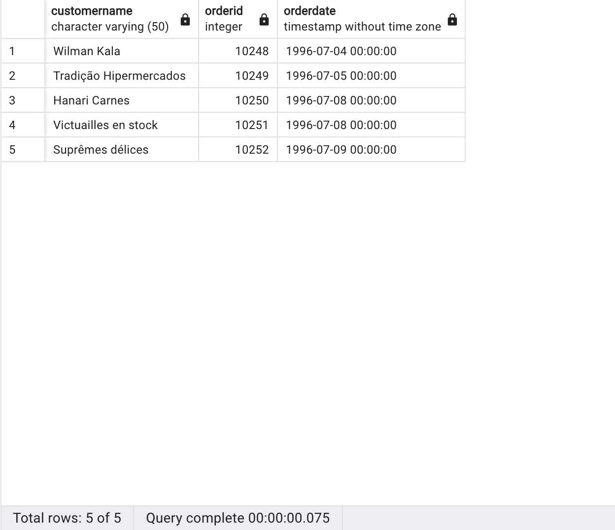
Query results from PgAdmin, Source Author
In summary, this query retrieves the customer name, order ID, and order date for the first five records where there is a matching customer ID between the customers and orders tables.
Inner joins can be used in various scenarios, from simple to complex queries involving multiple tables. They can also be combined with other SQL keywords, such as WHERE clauses and aggregate functions, to refine the result set further. Understanding how inner joins work can help write efficient and effective queries.
Left Outer Join
The LEFT OUTER JOIN, also known as simply a left loin, is a join operation in database management systems that returns all the rows from the Table1 and the matching rows from the Table 2. The result will contain NULL values if there is no match in the right table.
To provide more context, we will utilize our Northwind database and leverage the existing customer and orders tables in the following manner:
SELECT c.customerid, c.customername, o.orderid, o.orderdate
FROM customers c
LEFT OUTER JOIN orders o
ON c.customerid = o.customerid;
This query will return a result set that includes the customer ID, customer name, order ID, and order date for all customers, whether they have placed an order or not. A subset of the rows that will be returned are shown here:
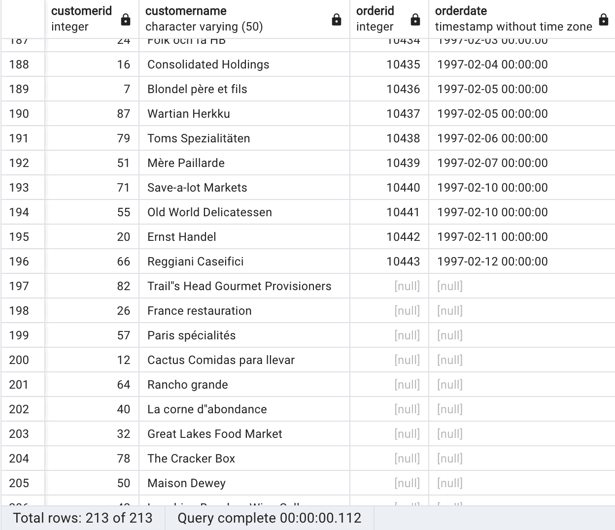
Query results, Source Author
If you order by the customername via the query
SELECT c.customerid, c.customername, o.orderid, o.orderdate
FROM customers c
LEFT JOIN orders o
   ON c.customerid = o.customerid
ORDER BY c.customername;
You will notice duplicates in the customername column because multiple orders from the same customer are present in the orders table. Since the query performs a LEFT JOIN between the customers and orders tables, it retrieves all rows from the customers table and matches them with corresponding rows from the orders table based on the customerid column. If a customer has placed multiple orders, their customer information (including the customername) will appear in multiple rows in the result set, each row representing a different order placed by that customer.
Using a LEFT JOIN in the previous query ensures that all records from the customers table will be included in the result set, regardless of whether there are matching records in the orders table. Using a LEFT JOIN, the query combines the data from the left table (customers) with matching records from the right table (orders) based on the specified join condition. If no matching records exist in the right table, NULL values are populated in the result set for the corresponding columns.
The advantage of this approach is that it allows us to retrieve customer data and any associated order information, but it’s worth noting that aggregating data with left join without taking account of the duplicates rows may lead to incorrect results.
Even if customers have not placed any orders, their information will still be included in the result set with NULL values in the order-related columns. Overall, the LEFT JOIN ensures that all customers are included in the result set, whether they have placed any orders. It provides a comprehensive view of customer data, incorporating relevant order information where available while maintaining the integrity of the customer records.
There are several benefits to using left outer joins in database management systems:
- Complete data retrieval from primary table: Left outer joins allow for complete retrieval of data from a primary table even if there is no matching data in a related table. This ensures that all records from the primary table are included in the result set, even if no corresponding data exists in the related table.
- Improved data analysis: Left outer joins can help to identify gaps or missing data in a related table, data quality assessment and aid improved data analysis and more informed decision-making.
By including data from the left table that may not have any matching records in the right table, left outer joins to enable us to retrieve data from multiple tables. Understanding how left-outer joins work and their benefits can help us write efficient and effective queries.
Right Outer Join
A Right Outer Join, also known as a Right Join, is a type of SQL join that reverses the roles of the two tables compared to in Left Outer Join. While a Left Outer Join ensures all records from the left (or primary) table are included in the result set, a Right Outer Join ensures all records from the right (or secondary) table are retained, regardless of whether there are matching records in the left table. This reversal makes the Right Outer Join particularly useful when you want to prioritize the data from the right table while incorporating any corresponding data from the left table.
Full Outer Join
A full outer join in SQL, also known as a full join, is a join operation that merges the output of left and right outer joins to make sure no data is lost in the join.
For instance, if we have two tables, Table A and Table B, and wish to join them on a common field called “ID“, a full outer join will include all rows from both tables, filling in NULL values where there is no corresponding match (and duplicating some of the rows much like we discussed in the Left Outer Join section earlier). To illustrate this concept, we will use the order table and the orderdetails table. These tables contain information about orders and the corresponding details of each order.
SELECT c.postalcode, o.orderid
FROM customers c
   FULL OUTER JOIN orders o
      ON c.customerid=o.customerid
ORDER BY c.customername;
This returns the following
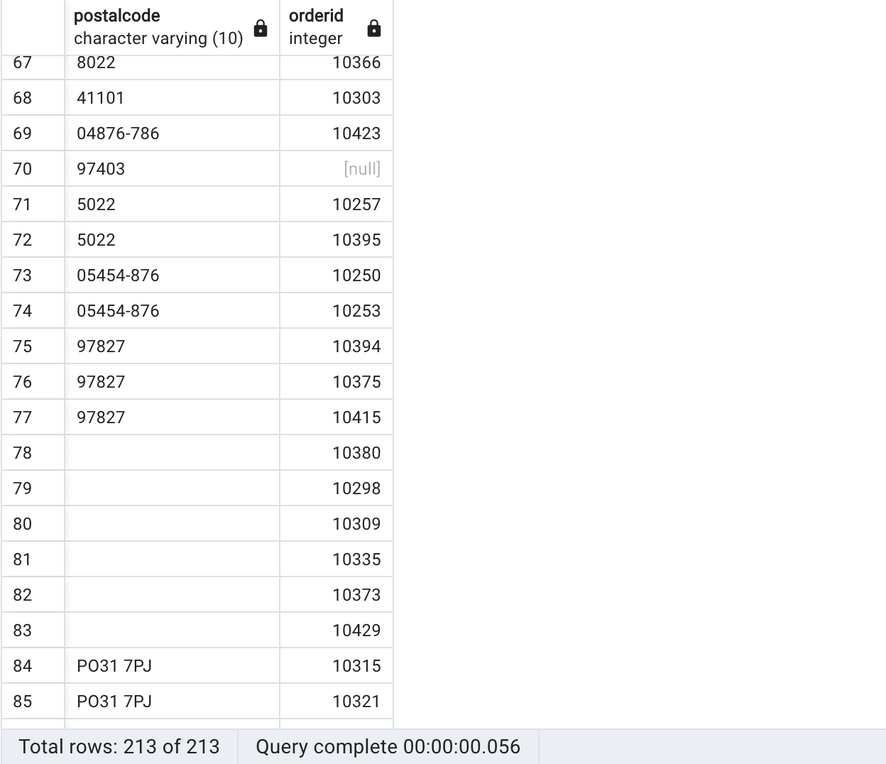
Query results, Source Author
The FULL OUTER JOIN ensures that all records from both tables are included in the result set, regardless of whether there is a matching record in the other table. This means that the query will return the combination of data from both tables, and any records that do not have corresponding matches in the other table will be included with NULL values in the respective columns. In the result set, we can see that the FULL OUTER JOIN includes all postal codes from the customers table and all order IDs from the orders table, including NULL records from joined fields from both tables.
Note too that there were duplicated postal code values, and that some of the postal code values are the empty string ‘’, which is semantically different from NULL.
Full outer joins in database management systems offer several benefits when working with relational data:
- Comprehensive data merging: Full outer joins allow you to combine all rows from two related tables, regardless of whether there is a match between the tables. This provides a complete picture of the data in both tables, making it easier to analyze and work with the combined dataset.
- Identify data discrepancies: Full outer joins can help identify mismatches or inconsistencies between two tables. When a full outer join is performed, and there is no match for a row from one table, the result will still include that row, but with
NULL values for the columns from the other table. These NULL values can indicate missing or inconsistent data, which can be helpful for data validation and cleanup.
- Simplify complex queries: A full outer join can sometimes simplify complex queries that would otherwise require multiple steps or a combination of different join types (e.g., left and right outer joins). You can retrieve all the necessary data in a single query using a full outer join, making the code more readable and easier to maintain. For instance, in the example query, we can utilize a Full Outer Join to identify orders without an associated postcode. This information can be used to identify orders that doesn’t have an associated postcode that can affect the delivery process .
- Flexible data analysis: Full outer joins offer flexibility when analyzing data from multiple tables. They enable you to retrieve information from both tables regardless of matching conditions, which can be particularly useful when working with optional relationships or when analyzing data that may not have a direct association.
Cross Join
A cross join, also known as a Cartesian join or Cartesian product, is a join operation in SQL that combines all rows from two tables without any condition. A Cross Join can be considered a specialized type of JOIN where the join condition always evaluates to TRUE, combining all rows from both tables.
Unlike other join operations that depend on specific matching conditions defined in the ON clause, a CROSS JOIN generates all possible combinations of rows from the involved tables. As noted in the overview section, this implies that any type of JOIN can inadvertently lead to a cross join if not written correctly. In other words, each row from the first table is paired with every row from the second table, resulting in a new table containing all possible combinations of rows from the original tables. The number of rows in the result set of a cross join equals the product of the number of rows in the first table and the number of rows in the second table. For example, if we have Table A with m rows and Table B with n rows, a Cross Join will return m * n rows, where each row from Table A is combined with each row from Table B.
Let’s perform a cross-join between the products and categories tables in the Northwind database. This will give us all the possible combinations of products and categories, even if the product does not belong to a specific category. Although this example might need to be revised in a real-world scenario, it demonstrates the concept of cross-joins using the existing product and categories.
SELECT p.productid, p.productname, c.categoryid, c.categoryname
FROM "products" p
CROSS JOIN "categories" c;
This returns the following (or at least a subset of what is returned because it is too large for the article):
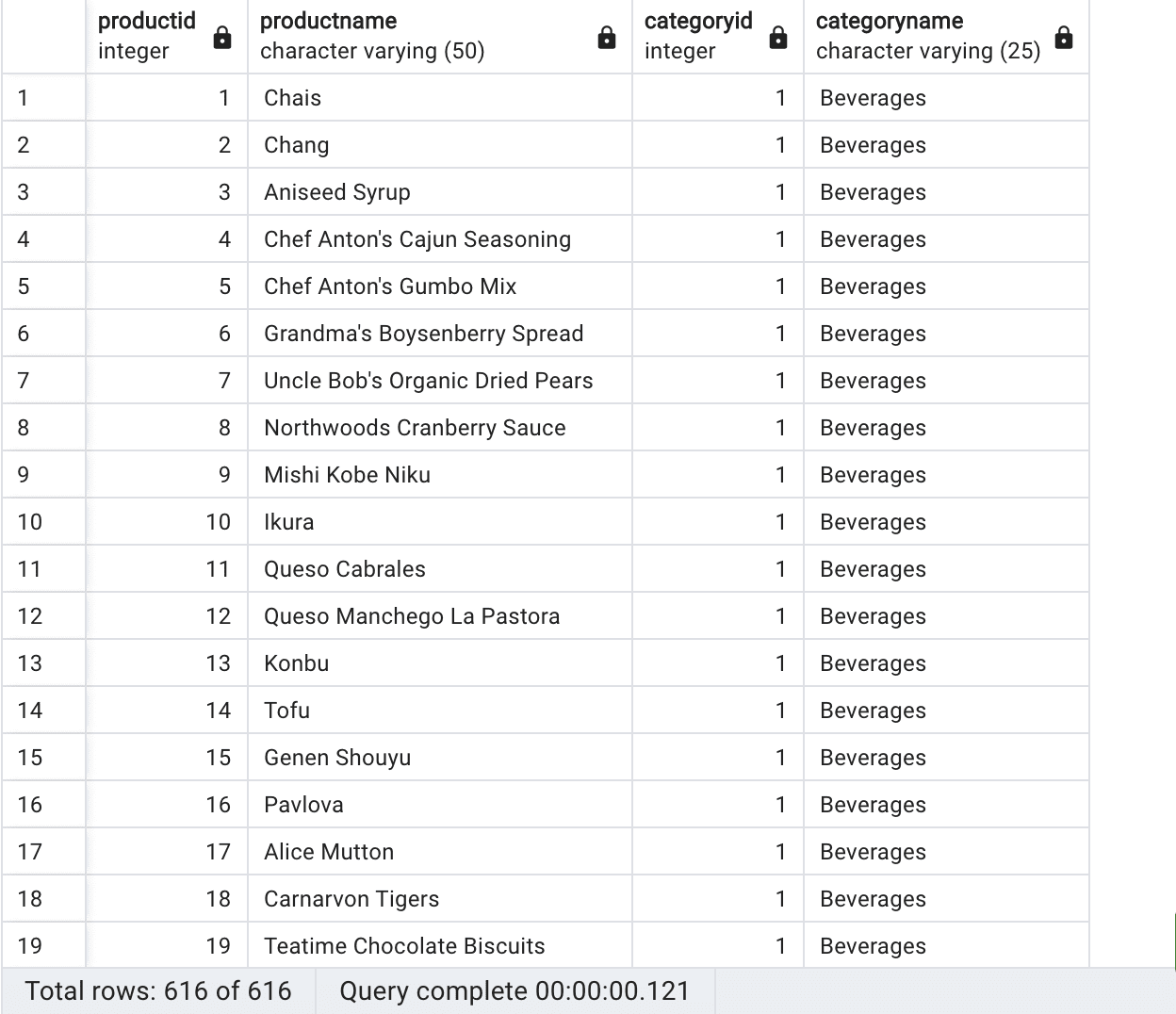
Query results, Source Author
The CROSS JOIN in this query combines all rows from the products and categories tables, resulting in a Cartesian product of the two tables. This means that the result set will include every possible combination of products and categories, even if the product does not belong to the category. For example, if there are 10 products and 5 categories, the result set will contain 50 rows, one for each combination of a product and a category. Each row will contain the product ID, product name, category ID, and category name. This query is useful for getting a comprehensive overview of all products and categories, regardless of their relation. For example, this query could be used to identify products that could be added to new categories or to identify categories that could be expanded to include new products.
Cross joins in database management systems have specific use cases and benefits when working with relational data:
- Generate all possible combinations: Cross joins produce a Cartesian product between two tables, creating all possible combinations of rows from the first table with rows from the second table. This can be useful in scenarios where you must explore all possible pairings or scenarios between two data sets.
- Add one row to a all the other rows in a set. For example, you might
CROSS JOIN to a single row of computation factors to have it available in every row in your table.
- Support for testing and data generation: Cross joins can be helpful in testing and generating sample data for various scenarios. For example, you can use a cross-join to create a dataset with all possible product options and configuration combinations, which can then be used for testing, analysis, or data modeling.
- Solve complex problem: In some cases, a cross-join can simplify complex queries or calculations that would require multiple steps or custom code. For example, you might use a cross-join to generate all combinations of input parameters for a query, allowing you to evaluate all possible scenarios in a single pass.
- Create combinations for decision support: Cross joins can generate all possible combinations of decision variables in decision support systems or optimization problems. This can help identify optimal solutions, evaluate trade-offs, and explore the solution space more effectively.
It’s important to note that cross-joins are only sometimes the most efficient or appropriate choice for every scenario. They can produce many rows in the result set, combining every row from the first table with every row from the second table. This can lead to performance issues or unnecessary complexity in your query. In most real-world scenarios, you would typically use other join types like inner, left, or right to retrieve more relevant and related data.
Self Join
A self-join is not a type of join configuration but a technique in SQL where a table is joined to itself, usually using an alias to differentiate between the original table and its copy. A self Join works by treating a table as two separate tables and joining them together. Self-joins are used to establish a relationship between rows within the same table based on a particular condition.
Here’s an example of a self-join using the Northwind database. In this example, we’ll use a self-join on the employees table:
SELECT
    e1.first_name AS EmployeeFirstName,
    e1.last_name AS EmployeeLastName,
    e2.first_name AS ManagerFirstName,
    e2.last_name AS ManagerLastName
FROM
    employees e1
LEFT JOIN
    employees e2 ON e1.reports_to = e2.employee_id
ORDER BY
    ManagerFirstName, EmployeeFirstName;
This will return the following, again truncated results:
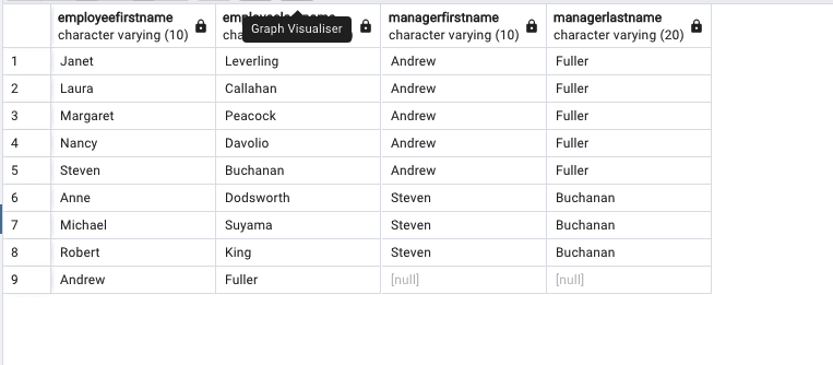
Query results, Source Author
This query retrieves a list of employees along their respective managers (who they report to) from the employees table. Since we are using a LEFT JOIN employees without managers will still appear in the result but will NULL values as seen above.
Benefits of using self-joins in database management systems:
- Retrieve hierarchical data: Self-joins are particularly useful when working with hierarchical data, where rows in the table have parent-child relationships. In such cases, self-joins can be used to retrieve the hierarchy or lineage of records.
- Retrieve indirect relationships: Self-joins can be used to retrieve indirect relationships between rows in the same table, such as finding common connections or shared attributes between records. For example, imagine the “Employee” table had a “supervisorid” field, we can use a self join to identify common/shared supervisor by different employees. For example:
SELECT e1.EmployeeName AS Employee1,
       e2.EmployeeName AS Employee2,
       e1.SupervisorID AS CommonSupervisorID
FROM Employees e1
     JOIN Employees e2
      ON e1.SupervisorID = e2.SupervisorID
Natural Join
A natural join is a join operation in SQL that automatically combines two tables based on columns with the same name and data type in both tables. A natural join is a shorthand for joining on columns with the same name.
SELECT c.customername, o.orderid, o.orderdate
FROM customers c
      NATURAL JOIN orders o
This returns the following based on the shared column orderid.
In a natural join, the database management system identifies columns with matching names and data types in both tables and uses these columns as the basis for the join condition. The natural join eliminates duplicate columns in both tables, returning only one copy of each matching column in the result set. It is important to note that natural joins can be risky, as they rely on column names and data types rather than explicitly defined join conditions. If you share names other than the relationship key values, this can make it impossible to use a NATURAL JOIN.
This can lead to unintended results if the table column names are unique and descriptive. Most modern database management systems, such as PostgreSQL, SQL Server, and Oracle, do not support natural joins directly in their SQL syntax. Instead, they require you to explicitly define the join conditions using an INNER JOIN, LEFT JOIN, or RIGHT JOIN with the ON clause.
However, some databases, like MySQL, support the NATURAL JOIN keyword. In general, it’s recommended to use explicit join conditions (e.g., INNER JOIN with the ON clause) instead of relying on natural joins, as this approach ensures that you have full control over the join operation and reduces the likelihood of unintended results (like if someone does add a new column to a table and that has the same name that your code has used a NATURAL JOIN in).
Combination of Joins
Combining different types of joins can significantly enhance the accuracy, performance, and readability of SQL queries. Let’s explore the power of join combinations using an example query that retrieves customers with orders and order details if there are any.:
SELECT c.customerid, c.customername, o.orderid, o.orderdate, p.productname
FROM Customers c
    INNER JOIN Orders o
       ON c.customerid = o.customerid
    LEFT JOIN OrderDetails od
       ON o.orderid = od.orderid
    INNER JOIN Products p
       ON od.productid = p.productid;
This returns the following:
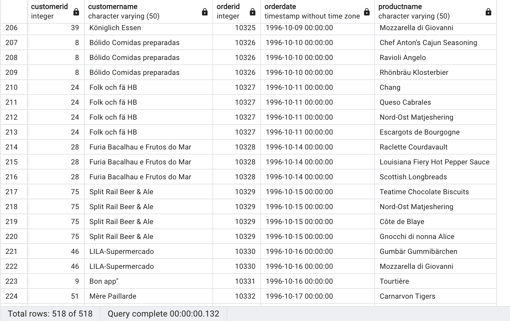
Query results, Source Author
First, an inner join is performed between the Customers and Orders tables using the CustomerID column. This ensures that only customers who have placed orders are included in the result. Next, a left join is applied between the Orders and OrderDetails tables using the OrderID column. This allows all orders to be included in the result regardless of whether they have corresponding order details. Finally, an inner join is executed between the OrderDetails and Products tables using the ProductID column. This ensures that only order details with valid product information are included in the result.
To summarize the query:
Customers and Orders tables are joined using an inner join on CustomerID.Orders and OrderDetails tables are joined using a left join on OrderID.OrderDetails and Products tables are joined using an inner join on ProductID.- The
SELECT clause specifies the columns to be retrieved: CustomerID, CustomerName, OrderID, OrderDate, and ProductName.
The second join actually join to the set formed by the Customer and Order table, so while in most cases you will join to the columns of just one table, it is possible that your join to the OrderDetails table could use Customers columns in the criteria. It is beyond the scope of this article to include more details.
By leveraging this combination of joins, businesses gain access to more comprehensive result sets that foster various analyses, such as order analysis, inventory management, product performance analysis, pricing, and profitability analysis. The retrieved data empowers data-driven decision-making and optimization of operations in a competitive marketplace. The use of join combinations, as demonstrated in this example query, allows businesses to uncover valuable insights and make informed decisions. It enhances the depth and breadth of information retrieved from multiple tables, enabling comprehensive analysis and optimization. By leveraging these combined joins, businesses can unlock hidden patterns, understand customer behavior, and drive success in their operations.
Conclusion
SQL joins are an essential component of database management that can make queries more efficient and productive. Understanding the different types of joins, including the inner, left outer, right outer, full outer, cross, self, natural joins, and combination of joins, can provide a significant advantage to anyone working with data.
By using PostgreSQL, individuals can practice and experiment with different types of joins in enhancing their data analysis skills. With the benefits of SQL joins, including increased productivity and improved data accuracy, mastering this skill can make a significant difference in data management. Therefore, we encourage our readers to continue practicing and exploring SQL joins to become proficient in database management.
The post Understanding SQL Join Types appeared first on Simple Talk.
from Simple Talk https://ift.tt/ROMCn7i
via
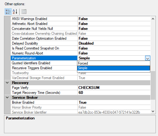
 One of the main claims is that when the same query is sent with different values, it is understood as two ad hoc queries. The DBA can’t see their plan to make any optimization, creating a problem.