AWS Lambdas with C#

Serverless computing is pushing C# to evolve to the next level. This is exciting because you pay-per-use and only incur charges when the code is running. This means that .NET 6 must spin up fast, do its job, then die quickly. This mantra of birth and rebirth pushes developers and the underlying tech to think of innovative ways to meet this demand. Luckily, the AWS (Azure Web Services) serverless cloud has excellent support for .NET 6.

In this article, I will take you through the development process of building an API on the serverless cloud with C#. This API will be built to serve pizzas, with two endpoints, one for making pizza and the other for tasting fresh pizzas. I expect some general familiarity with AWS and serverless computing. Any previous experience with building APIs in .NET will also come in handy.

Feel free to follow along because I will guide you through this step-by-step. If you get lost, the full sample code can be found on GitHub.

Getting the AWS CLI Tool

First, you will need the following tools:

• AWS CLI tool
• .NET 6 SDK
• Rider, Visual Studio 2022, Vim, or an editor of choice

The AWS CLI tool can be obtained from the AWS documentation. You will need to create an account then set up the CLI tool with your credentials. The goal is to configure the credentials file under the AWS folder and set an access key. You will also need to set the region depending on your physical location. Because this is not an exhaustive guide on getting started, I will leave the rest up to you the reader.

Create a New Project

I will pick the .NET 6 CLI tool because it is the most accessible to everyone. You can open a console via Windows Terminal or the CMD tool. Before you begin, verify that you have the correct version installed on your machine.

> dotnet --version

This outputs version 6.0.42 on my machine. Next, you will need the AWS dotnet templates:

> dotnet new -i Amazon.Lambda.Templates
> dotnet tool install -g Amazon.Lambda.Tools

If you have already installed these templates, simply check that you have the latest available:

> dotnet tool update -g Amazon.Lambda.Tools

Then, create a new project and a test project with a region.

> dotnet new serverless.AspNetCoreMinimalAPI -n Pizza.Api \
    --profile default --region us-east-1

> dotnet new xunit -n Pizza.Api.Tests

Be sure to set the correct region, one that matches your profile in the AWS CLI tool.

The dotnet CLI generates a bunch of files and puts them all over the place. I recommend doing a bit of manual clean up and follow the folder structure below in Figure 1.

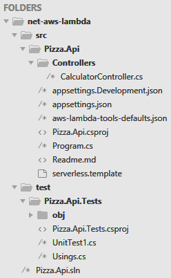
Figure 1. Folder structure

You may also create the solution file Pizza.Api.sln via:

> dotnet new sln -n Pizza.Api
> dotnet sln add src\Pizza.Api\Pizza.Api.csproj
> dotnet sln add test\Pizza.Api.Tests\Pizza.Api.Tests.csproj

This allows you to open the entire solution in Rider, for example, to make the coding experience much richer.

The template generated nonsense like a Controllers folder and HTTPS redirect. Simply delete the Controllers folder in the Pizza.Api folder and delete the UnitTest1.cs file that is in the Pizza.Api.Tests folder.

In the Program.cs file delete the following lines of code.

builder.Services.AddControllers();

app.UseHttpsRedirection();
app.UseAuthorization();
app.MapControllers();

The HTTPS redirect is a pesky feature that only applies to local to make life harder for developers. On the AWS cloud, the AWS Gateway handles traffic before it calls into your lambda function. Gutting dependencies also helps with cold starts. Trimming middleware like Controllers and Authorization keeps the request pipeline efficient because you get billed while the code is running. One technique to keep costs low, for example, is to use Cognito instead of doing auth inside the lambda function.

Run Your Lambda on Local

Luckily, .NET 6 makes this process somewhat familiar to .NET developers who are used to working with on-prem solutions. Be sure to have (or create) the following launchSettings.json under a Properties folder in the project:

{
  "$schema": "https://json.schemastore.org/launchsettings.json",
  "profiles": {
    "Pizza.Api": {
      "commandName": "Project",
      "dotnetRunMessages": true,
      "launchBrowser": false,
      "applicationUrl": "http://localhost:5095",
      "environmentVariables": {
        "ASPNETCORE_ENVIRONMENT": "Development"
      }
    }
  }
}

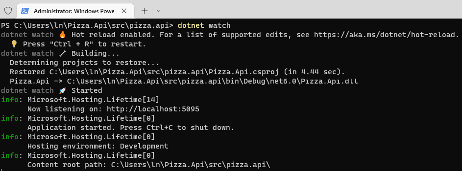
Now, go back to the console and run the app under the ..\Pizza.Api\src\Pizza.Api folder:

> dotnet watch

There should be an output telling you it is now running under the port number 5095.

This watcher tool automatically hot reloads, which is a nice feature from Microsoft, this is to keep up with code changes on the fly without restarting the app. This is mostly there for convenience, so I recommend keeping an eye out to make sure the latest code is actually running.

Then, use CURL to test your lambda function on local, make sure the -i flag remains lowercase or try –include:

> curl -X GET -i -H "Accept: application/json" http://localhost:5095

With the AWS tools, developers who are familiar with .NET should start to feel more at home. This is one of the niceties of the ecosystem, because the tools remain identical on the surface.

The one radical departure so far is using the minimal API to host an endpoint and I will explore this topic next.

Make a Pizza

To make a pizza, first, you will need to install the DynamoDB NuGet package in the project. (If you are not acquainted with Amazon DynamoDB, you can get more information here)

In the same Pizza.Api folder, install the dependency:

> dotnet add package AWSSDK.DynamoDBv2

Also, this project requires a Slugify dependency. This will convert a string, like a pizza name, into a unique identifier we can put in the URL to find the pizza resource in the API.

To install the slugify dependency:

> dotnet add package Slugify.Core

With lambda functions, one goal is to keep dependencies down to a minimum. You may find it necessary to copy-paste code instead of adding yet another dependency to keep the bundle size small. In this case, I opted to add more dependencies to make writing this article easier for me.

Create a Usings.cs file in the Pizza.Api directory in src and put these global usings in:

global using Amazon;
global using Amazon.DynamoDBv2;
global using Amazon.DynamoDBv2.DataModel;
global using Pizza.Api;
global using Slugify;

Now, in the Program.cs file wire up dependencies through the IoC container:

builder.Services.AddSingleton<IAmazonDynamoDB>( _ =>
  new AmazonDynamoDBClient(RegionEndpoint.USEast1));
builder.Services.AddSingleton<IDynamoDBContext>(p =>
  new DynamoDBContext(p.GetService<IAmazonDynamoDB>()));
builder.Services.AddScoped<ISlugHelper, SlugHelper>();
builder.Services.AddScoped<PizzaHandler>();

Note your region can differ from mine. I opted to use the DynamoDB object persistence model via the Amazon.DynamoDBv2.DataModel namespace to keep the code minimal. This decision dings cold starts a bit, but only a little. Here though, I am paying the cost of latency to gain developer convenience.

The DynamoDB object persistence model requires a pizza model with annotations so it can do the mapping between your C# code and the database table.

Create a PizzaModel.cs file, and put this code in:

namespace Pizza.Api;

[DynamoDBTable("pizzas")]
public class PizzaModel
{
  [DynamoDBHashKey]
  [DynamoDBProperty("url")]
  public string Url { get; set; } = string.Empty;

  [DynamoDBProperty("name")]
  public string Name { get; set; } = string.Empty;

  [DynamoDBProperty("ingredients")]
  public List<string> Ingredients { get; set; } = new();

  public override string ToString() =>
    $"{Name}: {string.Join(',', Ingredients)}";
}

Given the table definition above, create the DynamoDB table via the AWS CLI tool:

> aws dynamodb create-table --table-name pizzas \
      --attribute-definitions AttributeName=url,AttributeType=S \
      --key-schema AttributeName=url,KeyType=HASH \
      --provisioned-throughput ReadCapacityUnits=1,WriteCapacityUnits=1 \
     --region us-east-1 --query TableDescription.TableArn --output text

The url field is the hash which uniquely identifies the pizza entry. This is also the key used to find pizzas in the database table.

Next, create the PizzaHandler.cs file, and put in a basic scaffold:

namespace Pizza.Api;

public class PizzaHandler
{
  private readonly ISlugHelper _slugHelper;
  private readonly IDynamoDBContext _context;
  private readonly ILogger<PizzaHandler> _logger;

  public PizzaHandler(
    IDynamoDBContext context,
    ISlugHelper slugHelper,
    ILogger<PizzaHandler> logger)
  {
    _context = context;
    _slugHelper = slugHelper;
    _logger = logger;
  }

  public async Task<IResult> MakePizza(PizzaModel pizza)
  {
    throw new NotImplementedException();
  }

  public async Task<IResult> TastePizza(string url)
  {
    throw new NotImplementedException();
  }
}

This is the main file that will serve pizzas. The focus right now is the MakePizza method.

Before continuing, create the PizzaHandlerTests.cs file under the test project:

namespace Pizza.Api.Tests;

public class PizzaHandlerTests
{
  private readonly Mock<IDynamoDBContext> _context;
  private readonly PizzaHandler _handler;

  public PizzaHandlerTests()
  {
    var slugHelper = new Mock<ISlugHelper>();
    _context = new Mock<IDynamoDBContext>();
    var logger = new Mock<ILogger<PizzaHandler>>();

    _handler = new PizzaHandler(
      _context.Object,
      slugHelper.Object,
      logger.Object);
  }
}

The test project should have its own Usings.cs file, add these global entries:

global using Moq;
global using Amazon.DynamoDBv2.DataModel;
global using Microsoft.Extensions.Logging;
global using Slugify;

Also, install the Moq dependency under the Pizza.Api.Tests project:

> dotnet add package Moq

You will also need the Slugify and Amazon.DynamoDBv2 packages seen in the Pizza.Api project as well. First, I like to unit test my code to check that my reasoning behind the code is sound. This is a technique that I picked up from my eight-grade teacher: “test early and test often”. The faster the feedback loop is between code you just wrote and a reasonable test, the more effective you can be in getting the job done.

Inside the PizzaHandlerTests class, create a unit test method:

[Fact]
public async Task MakePizzaCreated()
{
  // arrange
  var pizza = new PizzaModel
  {
    Name = "Name",
    Ingredients = new List<string> {"toppings"}
  };

  // act
  var result = await _handler.MakePizza(pizza);

  // assert
  Assert.Equal("CreatedResult", result.GetType().Name);
}

There is a little quirkiness here because the Results class in minimal API is actually hidden behind private classes. The only way to get to the result type is via reflection, which is unfortunate because the unit test is not able to validate the strongly typed class. Hopefully in future LTS (Long Term Support) releases the team will fix this odd behaviour.

Now, write the MakePizza method in the PizzaHandler to pass the unit test:

public async Task<IResult> MakePizza(PizzaModel pizza)
{
  if (string.IsNullOrWhiteSpace(pizza.Name)
    || pizza.Ingredients.Count == 0)
  {
    return Results.ValidationProblem(new Dictionary<string, string[]>
    {
      {nameof(pizza), new [] 
                {"To make a pizza include name and ingredients"}}
    });
  }

  pizza.Url = _slugHelper.GenerateSlug(pizza.Name);

  await _context.SaveAsync(pizza);
  _logger.LogInformation($"Pizza made! {pizza}");

  return Results.Created($"/pizzas/{pizza.Url}", pizza);
}

With minimal API, you simply return an IResult. The Results class supports all the same behaviour you are already familiar with from the BaseController class. The one key difference is there is a lot less bloat here which is ideal for a lambda function that runs on the AWS cloud.

Finally, go back to the Program.cs file and add new endpoints right before the app.Run.

using (var serviceScope = app.Services.CreateScope())
{
  var services = serviceScope.ServiceProvider;
  var pizzaApi = services.GetRequiredService<PizzaHandler>();

  app.MapPost("/pizzas", pizzaApi.MakePizza);
  app.MapGet("/pizzas/{url}", pizzaApi.TastePizza);
}

One nicety from minimal API is how well this integrates with the existing IoC container. You can map requests to a method, and the model binder does the rest. Those of you familiar with Controllers should see code that reads identical in the PizzaHandler.

Then, make sure the dotnet watcher CLI tool is running the latest code and test your endpoint via CURL:

> curl -X POST -i -H "Accept: application/json" ^
    -H "Content-Type: application/json" ^
    -d "{\"name\":\"Pepperoni Pizza\",\"ingredients\":[\"tomato sauce\",\"cheese\",\"pepperoni\"]}" http://localhost:5095/pizzas

Feel free to play with this endpoint on local. Notice how the endpoint is strongly typed, if you pass in a list of ingredients as raw numbers then validation fails the request. If there is data missing, validation once again kicks the unmade pizza back with a failed request.

You may be wondering how the app running on local is able to talk to DynamoDB. This is because the SDK picks up the same credentials used by the AWS CLI tool. If you can access resources on AWS, then you are also able to point to DynamoDB using your own personal account with C#.

Taste a Pizza

With a fresh pizza made, time to taste the fruits of your labor.

In the PizzaHandlerTests class, add this unit test:

[Fact]
public async Task TastePizzaOk()
{
  // arrange
  _context
    .Setup(m => m.LoadAsync<PizzaModel?>("url", default))
    .ReturnsAsync(new PizzaModel());

  // act
  var result = await _handler.TastePizza("url");

  // assert
  Assert.Equal("OkObjectResult", result.GetType().Name);
}

This only checks the happy path; you can add more tests to check for failure scenarios and increase code coverage. I’ll leave this as an exercise to you the reader, if you need help, please check out the GitHub repo.

To pass the test, put in place the TastePizza method inside the PizzaHandler:

public async Task<IResult> TastePizza(string url)
{
  var pizza = await _context.LoadAsync<PizzaModel?>(url);

  return pizza == null
    ? Results.NotFound()
    : Results.Ok(pizza);
}

Then, test this endpoint via CURL:

> curl -X GET -i -H "Accept: application/json" http://localhost:5095/pizzas/pepperoni-pizza

Onto the Cloud!

With a belly full of pizza, I hope nobody feels hungry, deploying this to the AWS cloud feels seamless. The good news is that the template already does a lot of the hard work for you so you can focus on a few key items.

First, tweak the serverless.template file and set the memory and CPU allocation. Do this in the JSON file:

{
  "Properties": {
    "MemorySize": 2600,
    "Architectures": ["x86_64"]
  }
}

This sets a memory allocation of 2.5GB, with a x86 processor. These allocations are not final because you really should do monitoring and tweaking to figure out an optimal allocation for your lambda function. Increasing the memory blindly does not guarantee best results, luckily there is a nice guide from AWS that is very helpful.

Before you can deploy, you’ll need to create an S3 bucket which is where the deploy bundle will go. Note that you may need to provide your own name for the S3 bucket:

> aws s3api create-bucket --acl private --bucket pizza-api-upload \
    --region us-east-1 --object-ownership BucketOwnerEnforced
> aws s3api put-public-access-block --bucket pizza-api-upload \
    --public-access-block-configuration "BlockPublicAcls=true,IgnorePublicAcls=true,BlockPublicPolicy=true,RestrictPublicBuckets=true"

Then, deploy your app to the AWS cloud via the dotnet AWS tool:

> dotnet lambda deploy-serverless --stack-name pizza-api --s3-bucket pizza-api-upload

Unfortunately, the dotnet lambda deploy tool does not handle role policies for DynamoDB automatically. Login into AWS, go to IAM, click on roles, then click on the role the tool created for your lambda function. It should be under a logical name like pizza-api-AspNetCoreFunctionRole-818HE2VECU1J.

Then, copy this role name, and create a file dynamodb.json with the access rules:

{
  "Version": "2012-10-17",
  "Statement": [
    {
      "Action": [
        "dynamodb:DescribeTable",
        "dynamodb:GetItem",
        "dynamodb:PutItem",
        "dynamodb:UpdateItem"
      ],
      "Effect": "Allow",
      "Resource": "*"
    }
  ]
}

Now, from the Pizza.Api project folder, grant role access to DynamoDB via this command:

> aws iam put-role-policy --role-name pizza-api-AspNetCoreFunctionRole-818HE2VECU1J \
      --policy-name PizzaApiDynamoDB --policy-document file://./dynamodb.json

Be sure to specify the correct role name for your lambda function.

Finally, taste a pre-made pizza via CURL. Note that the dotnet lambda deploy tool should have responded with a URL for your lambda function. Make sure the correct GATEWAY_ID and REGION go in the URL.:

> curl -X GET -i ^
  -H "Accept: application/json" https://GATEWAY_ID.execute-api.REGION.amazonaws.com/Prod/pizzas/pepperoni-pizza

I recommend poking around in AWS to get more familiar with lambda functions.

The API Gateway runs the lambda function via a reverse proxy. This routes all HTTPS traffic directly to the kestrel host, which is the same code that runs on local. This is a bit more costly because the lambda function routes all traffic, but the developer experience is greatly enhanced by this. Go to S3 and find your pizza-api-upload bucket, notice the bundle size remains small, around 2MB. The dotnet AWS tool might be doing some trimming to keep cold starts low. Also, look at CloudWatch and check the logs for your lambda function. You will find cold starts in general are below .5 sec, this is great news! In .NET 6, the AWS team has been able to make vast improvements which I believe will continue in future LTS releases. Lastly, note the VM that executes the lambda runs on Linux, this is another area of improvement that is also possible in .NET 6.

Conclusion

AWS lambda functions with C# are now production ready. The teams from both Microsoft and AWS have made significant progress in .NET 6 to make this dream a reality.

 

The post AWS Lambdas with C# appeared first on Simple Talk.

from Simple Talk https://ift.tt/mg8Q1JC
via

Testing before coding: shifting farther left

Times have changed so much; when I wrote my first book on database design, I didn’t mention testing. In some respects, I thought it was obvious that everyone would gather requirements and test to make sure what they were building did what they expected. Let’s say I was younger then and considerably more naïve.

The Story

As a data architect, I typically found most of my problems in life just happened to occur less because of coding bugs and more because what I had designed didn’t match what the customer actually wanted. One of my first significant design mistakes came when designing a chemical plant QA system. Our analysts gathered requirements, gave them to the development team, and we implemented them. We did system testing and quality testing with the customer. There were poor time estimates, and cost overruns, but the software worked and worked, and our team believed it worked quite well.

Then we went live. There were lots of typical minor bugs, but everything was working great. Until the day the system would not let them do something that was out of the ordinary. One of the key requirements we were given was not to allow shipments if the material didn’t meet a certain quality. Eradicating previous quality issues was the central goal of this new system. What was not discussed was what happens if their customer wants to override that quality setting and take shipment anyhow? The team spent considerable time making sure that our system could not ship sub-standard product because that is what the requirements said.

The problem came down to the fact that we didn’t understand what the customer wanted in a way that cost them money. Delayed shipments and manual processing were required because the system wouldn’t allow them to do something that was apparently commonplace.

Test Very Early, Test Very Often

To fix this, I have always tried to test early, earlier, and earliest. Start before coding has started with the requirements. Find a way, in the customer’s language to verify that the requirements you have stated are accurate. Challenge requirements that are too specific. “We only see patients 18 years and younger” often means “We rarely see patients 18 years old and younger unless we decide to. In this case, there is a process that needs to be a part of the system, or it will be a horrible failure, but at least you will have a story to write about someday”.

It means getting representatives from the user community (not just upper-level management) to interact with the requirements that have been agreed upon and make sure they make sense. Challenge them to give you the odd (and very odd) along with typical cases. Some significant concerns happen once a year.

The farther you are left in the timeline, the easier it is to make changes. If it is still a document, just hit backspace and type the new requirement. If the business analyst had identified the override, or our team had asked the question “really, you can’t sell substandard materials to anyone?” money would have been saved.

The Process

Once we get to the “really sure” level of confidence that the requirements are correct, you can design more confidently. As a data professional, data models have a few natural checkpoints built into the process that can be very helpful. Start with a conceptual model that is just table names and projected relationships (the tables are concepts, hence the name conceptual model). Then test to make sure you can meet the requirements.

Take each requirement and just ask, “can I?” Can I store customer information? Can I represent an order? Can I represent an order of 10 products? 100 products? 10 orders in a minute? Not just the normal data you know of, but as many possibilities that could happen. Once you can meet that level of comfort with your model, you are getting close to a design that will only be decorated with attributes, not torn apart, and restarted over and over.

As you flesh out attributes, then start creating tables, constraints, etc., unit testing, integration testing, and then user acceptance testing are done hand in hand with the entire process. Every step of the way, verifying that what you have built meets the requirements you tested for veracity with the user community in the beginning.

Whether you are working in short sprints or long waterfall projects, the main difference is the amount of work you are doing. Continue this process of verification all the way through until you finish and start to work on the next thing.

Nothing is Ever Easy as It Sounds

The entire development process can be pretty easy except for the first step. Gathering requirements that meet what the customer wants a system to do is one of the most challenging jobs in existence that doesn’t require a Ph.D. in Mathematics. Why? Because most users are clueless as to how to tell you what they want most of the time. And the worst offenders think they know what they want without discussion.

Once you have requirements, designing and implementing software to meet well-written requirements is not necessarily trivial, but it is relatively straightforward. Luckily there is lots of software out there to help you with those tasks.

 

The post Testing before coding: shifting farther left appeared first on Simple Talk.

from Simple Talk https://ift.tt/QXzgeoY
via

Azure Functions and Managed Identity: More Secrets

I wrote about Managed Identity Secrets a few weeks ago, but since that article was published I made new interesting discoveries to add more to these secrets.

The combination of possibilities is considerable, and I faced two new situations I hadn’t faced before. Let’s discover the new secrets.

 

Storage Accounts and Triggers

The storage account triggers depend on configurations in the Function/App to stablish the connection.

This configuration is intended to contain a connection string built with a storage account key or SAS key.

When we want to use Managed Identities, the configuration needs to be different. The name we use in the trigger code becomes only the prefix for the configuration.

We need different configuration entries for the blob service and the queue service, each one containing the full address of the service. In this way, the trigger understands we intend to use Managed Identity authentication, instead of key/SAS authentication.

These are the names you should use for the configuration values:

<CONNECTION_NAME_PREFIX>__blobServiceUri

<CONNECTION_NAME_PREFIX>__queueServiceUri

Reference: https://learn.microsoft.com/en-us/azure/azure-functions/functions-bindings-storage-blob-trigger?tabs=in-process%2Cextensionv5&pivots=programming-language-csharp

Blobs Requires Queues

When you use keys, usually the connection string has the endpoint for all the services, blobs and queues.

When using managed identities, as explained above, the endpoint is in two different configurations. This brings up another secret: When connecting to a blob using the blob trigger, the queue connection is required as well.

The blob trigger handles failures using a queue, for this reason, when using the blob trigger the queue endpoint needs to be specified as well.

 

Azure SQL and User Managed Identities

The connection string for System Managed Identities is simple, as explained on the first article.

When using User Assigned Managed Identity, on the other hand, we need an additional parameter on the connection string. We need to specify the Client Id of the User Assigned Managed Identity we intend to use.

The Client Id is specified as the User Id. The connection string will be like this:

Server=DBServer.database.windows.net; Authentication=Active Directory Managed Identity; Initial Catalog=adventure;User Id=19fad297-5cf8-4fb9-9601-26d38d7854aa

This also applies to SQL Server 2022, which supports Azure AD Authentication.

 

Bonus: Using configurations to customize trigger parameters

Some trigger parameters are not so obviously configurable. For example, the queue name when connecting to a storage queue.

You wouldn’t like to have this kind of value tied in your code. The flexibility to change the queue name, for example, is very welcome. We can use different queue names for development, UAT and production environment, for example.

The solution is simple: you can use the ‘%’ symbol to retrieve a configuration value as a trigger parameter.

For example, a queue trigger would become like this:

[QueueTrigger(“%queuenameconfig%”, Connection = “inputStorage”)]

The connection parameter is retrieved from the configuration naturally, with the additional details explained above about managed identities. The queue name, on the other hand, will only the retrieved from configuration if transformed in a variable using the ‘%’ symbol.

 

Conclusion

Using Managed Identities on PAAS services can be full of tricks. Don’t assume a service doesn’t support it, you may be missing a configuration.

 

The post Azure Functions and Managed Identity: More Secrets appeared first on Simple Talk.

from Simple Talk https://ift.tt/DF5sT1f
via

PostgreSQL Basics: Roles and Privileges

Authentication	Authorization
Verify that the user is who they claim to be. This can be through password, trust, or some other federated login (like Kerberos)	As an authenticated user, what am I permitted to do within the system?

Before we get started, lets establish a few terms:

• Roles: There is only one type of authentication principal in PostgreSQL, a ROLE, which exists at the cluster level. By convention, a ROLE that allows login is considered a user, while a role that is not allowed to login is a group. Please note, while the CREATE USER and CREATE GROUP commands still exist, they are simply aliases for CREATE ROLE.
• Database Objects: Anything that can be created or accessed in the PostgreSQL cluster is referred to as an object. Databases, schema, tables, views, procedures, functions, and more can each have different privileges applied to them for any role.
• Privileges: The types of access that can be granted to a role for a database object. Often these will be applied at a database or schema level, but the ability to apply specific access to individual objects is always available. Privileges assigned to one role can be granted to other roles. This is typically done by granting group roles (those that cannot login) to user roles (those that can login) to assist with privilege management.

Depending on your previous experience with information security (within a database, operating system, or application), the way that these components work together in PostgreSQL may be different than you would expect.

Throughout this article you will see references to a PostgreSQL cluster. If you are new to PostgreSQL, this term may really confuse you. This is the way that PostgreSQL refers to the individual server/instance that’s running and hosting (a cluster of) databases. It does not mean that multiple servers are setup in a multi-node environment.

Principle of Least Privilege

One other key idea to discuss is the Principle of Least Privilege (PoLP), an information security methodology that states users should only be granted access to the least amount of information needed to do their job or task. Any access beyond files or data that they own must be specifically granted to them.

Although not stated specifically in documentation, many of the nuances of PostgreSQL security and how roles and privileges work together, feel like they are implemented with PoLP in mind.

For instance, only the owner of a database object (schema, table, function, etc.) can use or alter it unless specific access has been granted to other roles. For example, most users would probably expect that two roles with the same database or schema privileges (eg. SELECT) should be able to select from any table by default. That’s not how it works in PostgreSQL without some intervention.

Instead, objects are always owned by a role (and only one role) which must set privileges for other roles in most cases. This behavior can be modified so that new objects a role creates automatically grants specific privileges to other roles, but out of the box, object ownership is a key concept to understand when creating roles and other objects in a PostgreSQL database.

We’ll look at this more in a follow-up article on object ownership and privileges.

Superusers

One last thing to discuss before diving into role creation and granting privileges is the concept of a superuser. In PostgreSQL, a superuser is a role that is allowed to do anything in the system and is analogous to the root user in Linux or the sa account in SQL Server.

When a user has been granted superuser, no permission checks are performed when they execute SQL code (DDL/DML) or administer the cluster. The only check that is performed is whether they are allowed to login and connect to the cluster. Being designated as a superuser bypasses all other checks, including things like Row Level Security (RLS). This behavior is different than some other database systems.

To function properly, every PostgreSQL cluster needs to have at least one superuser to perform some administration tasks. Initially these tasks might be creating databases and additional roles, but there are a few tasks as of PostgreSQL 15 (installing some extensions, modifying some server parameters) that still require a superuser.

In PostgreSQL this initial superuser account is called postgres by default, which typically matches the system username that is running the PostgreSQL cluster process. This initial superuser can be changed using the initdb command to instantiate your own PostgreSQL cluster. That discussion is beyond the scope of this article but is generally not recommended without more experience.

One final note. If your PostgreSQL database is hosted with a service such as AWS RDS or Azure Postgres, you will probably not have access to a superuser role. Instead, the initial role that is created for you has most privileges needed to administer users and create databases and objects. Even if you host your own PostgreSQL cluster and have access to a superuser role, the recommendation (and documented best practice) is to create at least one role that has CREATE USER and CREATE DATABASE permissions but is not a superuser. With these role-specific attributes, a role can create new users (or another database), but not bypass other security checks like selecting data from tables that they don’t have permission to. This will allow you to do almost all administrative tasks without the ability to bypass all privilege checks while working in the database or cluster.

PostgreSQL Roles

Recall that in PostgreSQL both users and groups are technically roles. These are always created at the cluster level and granted privileges to databases and other objects therein. Depending on your database background it may surprise you that roles aren’t created as a principal inside of each database. For now, just remember that roles (users and groups) are created as a cluster principal that (may) own objects in a database, and owning an object provides additional privileges, something we’ll explore later in the article.

For the purposes of this article, all example user roles will be created with password authentication. Other authentication methods are available, including GSSPI, SSPI, Kerberos, Certificate, and others. However, setting up these alternative methods is beyond what we need to discuss object ownership and privileges.

Create a User Role

To create a user role in PostgreSQL, execute the following DDL as a user that has the `CREATEROLE` privilege. As discussed above, this is typically the postgresql superuser or an administrative user provided by your hosting solution.

CREATE ROLE dev1 WITH LOGIN PASSWORD ‘supersecretpw’;

Alternatively, PostgreSQL still supports the older CREATE USER command, but it’s just an alias for CREATE ROLE. In theory it will be deprecated at some point, so users should tend towards CREATE ROLE.

-- This still works as of PostgreSQL 15. Same as above, 
-- but implicitly adds LOGIN
CREATE USER dev1 WITH PASSWORD ‘supersecretpw’;

At the most basic level, this is all that’s required to create a role that can login to the cluster. What they can do after authenticating depends on the privileges that you grant to them (which we’ll discuss in later in the article.)

Maintaining unique privileges among many user roles can be cumbersome and error prone. Therefore, it’s desirable to create roles that function as groups so that users can inherit group privileges as needed. For example, consider the following diagram:

If a role is a member of the reader role, they have SELECT privileges on the public.table_name object. If they are in the creator role, then INSERT privileges, too, because each of those roles was explicitly granted privileges to a resource. Role reader_and_creator, which has not explicitly been granted any privileges outside of the public role, does have SELECT and INSERT privileges on public.table_name because it has been granted membership in both reader and creator. By crafting roles in a very deliberate manner, you can manage user roles through inheritance rather than granting individual privileges to each user. This is very important because user roles will change in different environments (people who can modify DEV may not even have access to login to the PROD cluster, for example.)Create a Group Role<

To create a group role in PostgreSQL, create a role that is not allowed to login. As mentioned earlier, this is simply a convention that denotes the role as a group.

CREATE ROLE devgrp WITH NOLOGIN;

Like user roles, PostgreSQL still supports the older CREATE GROUP command, although it is a direct alias for CREATE ROLE because all roles are created with NOLOGIN by default, which as we’ve discussed, means the role is used as a group. There is no advantage of using CREATE GROUP and it may be deprecated at some point.

There are numerous other role attributes that can be applied at the time of creation or through ALTER ROLE. Let me highlight a few additional role attributes and their default values.

Role Attribute Options (Default Bold)	Description
SUPERUSER/NOSUPERUSER	Is this role also a superuser? Superuser roles are required to effectively run a PostgreSQL cluster but should be rare and limited in use. All other privileges and role attributes checks are bypassed for a superuser. (ie. Superusers can do anything in the system!) Only a superuser can create another superuser.
CREATEDB/NOCREATEDB	Can this role create databases on the given PostgreSQL cluster?
CREATEROLE/NOCREATEROLE	Is this role allowed to create additional roles (users or groups) on the PostgreSQL cluster?
INHERIT/NOINHERIT	Roles can be granted membership into other roles. If a role can inherit from another role, then they can automatically use privileges without having to switch roles, similar to how privileges work in operating and file systems. If the user does not INHERIT privileges of the “parent” group, then they must switch to that role (SET ROLE) in order to utilize specific privileges of the group.
LOGIN/NOLOGIN	Can this role authenticate and login to the cluster? LOGIN must be specifically specified to allow a new role to authenticate.

See the documentation for all possible attributes and more detailed more information. Also, any of these role attributes (including superuser) can be modified at any time with the ALTER ROLE command.

Now that we have roles, one of which can login (our user) and one that can’t (our group), we need to dive into how privileges are assigned and applied.

The PUBLIC Role

Every PostgreSQL cluster has another implicit role called PUBLIC which cannot be deleted. All other roles are always granted membership in PUBLIC by default and inherit whatever privileges are currently assigned to it. Unless otherwise modified, the privileges granted to the PUBLIC role are as follows.

PostgreSQL 14 and below	PostgreSQL 15 and above
CONNECT CREATE TEMPORARY EXECUTE (functions and procedures) USAGE (domains, languages, and types)	CONNECT TEMPORARY EXECUTE (functions and procedures) USAGE (domains, languages, and types)

The main thing to notice here is that the PUBLIC role always has the CONNECT privilege granted by default, which conveniently allows all roles to connect to a newly created database. Without the privilege to connect to a database, none of our newly created roles would be able to do much.

Connections to a PostgreSQL database cluster are always opened to a specific database, not just the cluster. Remember that we started this article talking about authentication and authorization. To open a connection to a PostgreSQL cluster, a user first needs to authenticate (provide credentials for a role WITH LOGIN) and then have authorization to connect to a database. Because every role is granted membership in the PUBLIC role and that role has the privilege to CONNECT by default, all roles that can authenticate are allowed to CONNECT to the database as well.

Many of these defaults can be modified. As a database administrator you could REVOKE the ability for the PUBLIC role to CONNECT and then grant it to each role individually, but the complexity of managing that is rarely worth the effort.

To be clear, this privilege only allows the user to connect and see high-level objects in the public schema (tables, for instance). However, they cannot select or modify anything from tables without further permission. We’ll talk about this in a bit.

There is one last thing I’d like to point out in the table above that lists default permissions for the PUBLIC role.

Notice that default privileges changed slightly in PostgreSQL 15 and above. Previously, the PUBLIC role was also allowed to CREATE objects in the public schema of a database, and every database has a public schema by default. This permission was granted to the public role many years ago for backwards compatibility with very old versions of PostgreSQL, but also presented a security vulnerability. With the rise of DBaaS services, the potential for a new role to create tables, triggers, and functions in the public schema meant that they could potentially execute code that would later result in the elevation of their privilege (or worse).

Therefore, starting with PostgreSQL 15, the public role can no longer create anything by default, regardless of the schema. While it means a bit more work for administrators, revoking the CREATE privilege has been a recommended best practice for a long time.

Testing The New Role

With the new user role we created, dev1, we can login to the PostgreSQL cluster with a tool like psql using the following command. In the following examples the PostgreSQL cluster is hosted locally on my laptop using Docker with the default port of 5432. Your connection details, including the database name, may be different and should be adjusted as necessary.

-- Using flags, you will be prompted for a password as 
-- there is no specific “password” flag
psql -h localhost -U dev1 -d postgres

-- Alternate using PostgreSQL connection URI
psql postgres://dev1:supersecretpw@localhost:5432/postgres

This will cause a prompt for a password (if you didn’t provide it through the URI) and will connect the user to the postgres database. It works because the dev1 role is automatically granted membership in the PUBLIC role, which in turn has permission to connect to the postgres database.

With password authentication and one DDL statement, we created a role and logged into the PostgreSQL instance. Not too difficult, right?

So now, let’s get to work developing a new feature as the newly created dev1 account!

Creating Objects With the New User

As a developer user my first order of business is to get to work creating the table required to support the new feature I’m working on. The feature requires a table to store social accounts for each user. I’m not sure how many social account handles we plan to support, so I’ll just start with a basic table that stores each handle in a separate column.

Depending on which version of PostgreSQL you’re connected to, this may or may not be as easy. Remember, PostgreSQL 14 and below allowed the PUBLIC role (which `dev1` is a member of) to CREATE in the public schema by default. PostgreSQL 15 and above, however, does not.

After logging in as `dev1`, we attempt to create the following table.

CREATE TABLE user_social (
   user_id INT NOT NULL,
   twitter_handle TEXT NULL,
   facebook_handle TEXT NULL );

In PostgreSQL 14 and below, this probably succeeds on most installations given the setup we’ve done so far. In PostgreSQL 15 and above, however, our dev1 user most likely receives the following error.

ERROR: permission denied for schema public
LINE 1: CREATE TABLE user_social (

Let me reiterate, this only works in PostgreSQL 14 and below because the PUBLIC role is granted the ability to CREATE objects in the public schema by default. We would receive a similar error if we tried to do something like create a new schema in the database because PUBLIC has not been granted the CREATE privileges for the entire database, only the public schema.

For reference, the CREATE privilege can be applied to three areas in PostgreSQL (database, schema, and tablespaces) and allow creation of different objects depending on where you have permission to CREATE, as outlined on the privileges page in the documentation.

Whether we need to create a table or a new schema, how do we ensure that new developer roles can do that?

We must GRANT them privileges.

Granting privileges to Roles

PostgreSQL has a robust set of privileges built in, all of which are outlined in the documentation. For the following examples we’re going to focus on granting the CREATE privilege to the dev1 user in PostgreSQL 15.

-- As a superuser or role that can grant this 
-- privilege to others
GRANT CREATE ON SCHEMA public TO dev1;

Now that we’ve granted CREATE to dev1, we can attempt to create our table again in PostgreSQL 15. We could keep multiple sessions open (either in psql or your IDE of choice), but another option is to use SET ROLE. You can “switch” to another role if you are logged in as a superuser or that you are a member of. This is helpful for things like setting the correct object ownership at creation time and for testing permissions like we’re doing here.

-- temporarily set role in the current session to a different 
--role. Only superusers or members of the role can do this.
SET ROLE dev1;

-- Create the table as dev1 given the new permissions
CREATE TABLE user_social (
   user_id INT NOT NULL,
   twitter_handle TEXT NULL,
   facebook_handle TEXT NULL );

-- set the role back to the session initiated role
SET ROLE NONE;

Success! We’re a step closer to adding this new feature to our application.

Unfortunately, we quickly run into the another problem. To develop this feature, our developer needs to select data in the `user` table, but attempting to do so results in another error:

-- set our role back again if connected through 
-- another user session
SET ROLE dev1;

-- execute a select query against another table
SELECT * FROM “user” u
INNER JOIN user_social usoc USING(user_id);

This returns:

ERROR: permission denied for table user

As you probably guessed, the solution is to grant another privilege to the dev1 role. As a superuser or role that has the ability to grant these privileges:

-- In this example, grant SELECT on ALL tables in the schema. 
-- We could be more selective if needed
GRANT SELECT ON ALL TABLES IN SCHEMA public TO dev1;

If we know all the privileges that our developers need to do their work, we can add multiple privileges at one time. For example, if a developer needs to SELECT, INSERT, UPDATE, and DELETE data in tables of the public schema, we could do this in one statement.

GRANT SELECT, INSERT, UPDATE, DELETE 
     ON ALL TABLES IN SCHEMA public TO dev1;

Let’s be honest, though. Managing privileges one at a time for each role from database to database is going to be a maintenance headache. As soon as we create an account for the next developer on our team, dev2, we’ll have to start this entire process over.

Surely there’s a better way to manage this.

Granting Privileges Using Groups

PostgreSQL provides the ability to grant the privileges of one role to another role. Specifically, group roles (the ones that cannot login) are the perfect mechanism for applying sets of privileges to many users at once.

Earlier we created a group role called devgrp. It’s not allowed to log in and we haven’t granted it any privileges yet. We could instead grant this role the privileges we want to provide to all developers and then grant the devgrp role to each of them. Then any time we need to tweak developer privileges we only have to modify (GRANT or REVOKE) privileges from the devgrp role.

-- As a superuser or role that has the ability to grant 
-- this privilege to others
GRANT CREATE ON SCHEMA public TO devgrp;

GRANT SELECT, INSERT, UPDATE, DELETE 
            ON ALL TABLES IN SCHEMA public TO devgrp;

And now, any role that we grant membership to will inherit these permissions by default.

GRANT devgrp TO dev1;

At this point dev1 inherits all privileges that devgrp has. Any time a new developer joins the team and requires access to the database, we can create a role and grant them membership in the devgrp role. This can be done at any time using the GRANT statement above or during role creation time if the group role already exists.

-- This will create the role and automatically add it as 
-- a member of the devgrp role
CREATE ROLE dev2 WITH LOGIN PASSWORD ‘supersecretpw2’ 
                                            IN ROLE devgrp;

Conclusion

PostgreSQL has a comprehensive role and privilege system that allows a lot of flexibility for managing access to server objects and resources. In this article we learned about roles, how to use them effectively to manage users and groups, and how to grant some initial privileges to the new roles that we created.

We also discussed the importance of superuser roles and that most DBaaS services will not provide you with a superuser because it bypasses all privilege checks. Instead, the best practice is to create one or more administrative users with CREATEROLE and CREATEDB privileges for day-to-day administration. If you use a service like AWS or Azure, the administrative user they provide likely has these privileges rather than being a full superuser.

Once we had created new roles, we briefly discussed how to GRANT privileges to new roles individually and through inheritance so that our new roles could do the work needed to develop a new application feature.

In a follow-up article, we’ll dig deeper into object ownership and how it plays an important role (pun intended) in how you set up and maintain object ownership in your applications. Understanding how object ownership impacts the way that scripts are run, and backups are managed, will help you design secure applications that are easier to manage.

The post PostgreSQL Basics: Roles and Privileges appeared first on Simple Talk.

from Simple Talk https://ift.tt/BhKyRnM
via

Manage Data Over Time with SQL Server MERGE Statement

This article is part of Greg Larsen's continuing series on Learning T-SQL. To see all 8 items in the series, click here.

The basic MERGE statement

The MERGE statement was introduced with SQL Server 2008. It provides a single statement to perform UPDATE, INSERT and/or DELETE operations against a target table. The syntax for the basic MERGE statement that will be discussed, in this article, can be found in Figure 1:

MERGE
[ INTO ] <target_table>

USING <table_source> [ [ AS ] table_alias ]
   ON <merge_search_condition>

[ WHEN MATCHED [ AND <clause_search_condition> ]
  THEN <merge_matched> ] [ ...n ]

[ WHEN NOT MATCHED [ BY TARGET ] [ AND <clause_search_condition> ]
  THEN <merge_not_matched> ]

[ WHEN NOT MATCHED BY SOURCE [ AND <clause_search_condition> ]
  THEN <merge_matched> ] [ ...n ];

Figure 1: Basic Merge Statement

Where:

• target_table – identifies the table or view from which rows will be matched, so the appropriate update, insert, or delete actions can be performed based on the matching criteria.
• table_source –identifies the data source rows for which target_table rows are matched.
• merge_search_condition – identifies the join criteria for matching target_table rows, with the source_table rows.
• merge_matched – identifies either an UPDATE or DELETE statement to issue based on matching criteria.
• merged_no_matched – identifies the INSERT statement to issue for each row not matched.
• clause_search_condition – identifies any valid search condition.

For the complete syntax of the MERGE statement refer to the Microsoft documentation that can be found here.

To better understand how the MERGE statement maintains a target table, a few merge examples will be provided, in the sections below. But first some test data needs to be created.

Creating Initial Test Data

To show how the MERGE statement works a new database will be created. The new database will contain tables that I will use as a target and source for the examples, which will be populated with the initial test data. The examples in this article will show how a fictious manufacturing company named Widget Magic keeps this data synchronized using different MERGE examples.

The code in Listing 1 is used to create a database, the target and source table, and populates these tables with some initial rows of data. Note if you don’t want to create a new database the source and target tables can be created in the tempdb database.

-- Create repository for products
CREATE DATABASE MergeDB
GO

USE MergeDB;

SET NOCOUNT ON;

CREATE TABLE dbo.ProductInventory (
   ID int identity, 
   ProductName varchar(20),
   Qty int);

CREATE TABLE dbo.ProductRun(
   RunNum int,
   ProductName varchar(20), 
   Qty int);
-- Product Run #1

USE MergeDB;
GO

INSERT INTO dbo.ProductRun (RunNum, ProductName, Qty) VALUES
   (1,'Widget Basic',5), 
   (1,'Widget Pro',5);
GO

INSERT INTO dbo.ProductInventory (ProductName, Qty) VALUES
   ('Widget Basic',5),
   ('Widget Pro', 5);
GO

Listing 1: Create repository for products

In Listing 1 two tables are created: dbo.ProductInventory and dbo.ProductRun. The dbo.ProductInventory table tracks the inventory of products created by Widget Magic company. Whereas, the dbo.ProductRun table will be used to keep track of the products produced from each product run cycle. The rows of data inserted into these two tables represents the products produced from the first product run of widget products. During that first product run 5 Widget Basic and 5 Widget Pro items were produced.

For the purpose of this article the dbo.ProductInventory table will be used as the target table of the MERGE examples. Whereas, records from the dbo.ProductRun table will be used as the source table records.

Merge Example #1 – Inserting/Updating Using MERGE Statement

In order to show how the MERGE statement works to maintain the dbo.ProductInventory table, the Widget Magic company first needs to have a second product run cycle. The second run produced 5 more Widget Pro items and introduced a new product called Widget Super Pro, of which 5 are produced

The code in Listing 2 inserts two new rows into the dbo.ProductRun table to represent the new products produced by this second product run.

-- Product Run #2
USE MergeDB;
GO

INSERT INTO dbo.ProductRun (RunNum, ProductName, Qty) VALUES
   (2, 'Widget Pro',5),
   (2, 'Widget Super Pro',5);
GO

Listing 2: Inserting Production Run #2 Rows

To update the dbo.ProductInventory table, based on the products manufactured during the second product run, the MERGE statement in Listing 3 will be run.

-- Merge Example #1 
USE MergeDB;
GO

MERGE dbo.ProductInventory AS T  
USING (SELECT * FROM dbo.ProductRun WHERE RunNum = 2) AS S 
ON T.ProductName = S.ProductName 
-- Perform UPDATE when rows are matched 
-- between source and target
WHEN MATCHED THEN 
   UPDATE SET T.Qty = T.Qty + S.Qty
-- Perform INSERT when rows are not matched 
--between source and target
WHEN NOT MATCHED BY TARGET THEN 
   INSERT (ProductName,Qty) VALUES (S.ProductName, S.Qty);

-- Review Inventory
SELECT * FROM dbo.ProductInventory;
GO

Listing 3: Merge Example #2 – Inserting/Updating ProductInventory table

Report 1 shows the rows in the dbo.ProductInventory table after the MERGE statement was executed.

Report 2: Output of SELECT statement in Listing 5

The MERGE statement in Listing 3 compares the dbo.ProductInventory records, with the widgets products produced during the second product run. The dbo.ProductInventory table is the target table, and the rows returned from the subquery “SELECT * FROM dbo.ProductRun WHERE ProductRun = 2” identifies the source rows. The target and source rows are joined based on the merge_search_condition specified with the “ON” clause, which in this case was “T.ProductName = S.ProductName”.

A word of caution here, target table columns should only be compared with source columns. Do not use any target table columns to filter out rows as part of the “ON” clause. Doing so could produce unexpected or incorrect results.

When rows are matched between target and source rows, SQL Server assigns a matching condition for each row, based on the merge_search_condition. When this condition equates to true, the source row is known as a MATCHED with a target row. When the merge search condition is false the source table row is considered “NOT MATCHED”. NOT MATCHED then is be broken into two different conditions “NOT MATCHED BY TARGET” and “NOT MATCHED BY SOURCE”.

The “NOT MATCHED BY TARGET” in this example means a row exists in the source table that did not match a row in table based on the join criteria. Whereas the “NOT MATCHED BY SOURCE” condition means that a row exists in the target table that has no matching rows in the source table (look at Example 2 for to see a “NOT MATCHED BY SOURCE” example). Additionally, when both source and target table comparison columns contain NULL values, the matching value is considered “NOT MATCHED” for both target and source tables.

For each row in source table from second product run, that got a MATCHED condition an UPDATE operation against the target table was performed. The UPDATE operation increases the inventory value of the Qty column, on the matched target row, based on the Qty column value, of the matching row in the source table.

An INSERT operation was performed for each source row, from the second product run that got a NOT MATCHED BY TARGET condition. The INSERT operation uses the source table’s ProductName and Qty values to insert a new rows into the target table for each new product produced.

Report 2 shows that 5 more Widget Pro and Widget Super Pro items were added to the dbo.ProductInventory table. This MERGE statement showed how to insert and update rows into the target table, based on a matching condition with the source table. The MERGE statement can also perform DELETE statements.

Merge Example #2 – Inserting/Updating/Deleting using MERGE Statement

The Widget Magic company so far has had two different product runs of their widget products. The Widget Basic product has not been well received, as the product has been demonstrated to potential customers. Therefore management has decided that this product should be removed from the inventory, once the next product run has completed.

For the third product run, only the Widget Pro, and Widget Super Pro items are produced. The code in Listing 6 inserts these products from product run #3 into the dbo.ProductRun table.

-- Product Run #3
USE MergeDB;
GO

INSERT INTO dbo.ProductRun (RunNum, ProductName, Qty) VALUES
   (3, 'Widget Pro',100),
   (3, 'Widget Super Pro',50);
GO

Listing 4: Inserting Product Run #3 Rows

To show how the MERGE statement can insert, update, and delete rows from a target table, the code in Listing 5 merges will be run.

-- Merge Example #2 
USE MergeDB;
GO

MERGE dbo.ProductInventory AS T  
USING (SELECT * FROM dbo.ProductRun WHERE RunNum = 3) AS S 
ON T.ProductName = S.ProductName 
AND S.RunNum = 3
-- Perform UPDATE when both target and source MATCHED 
WHEN MATCHED THEN 
   UPDATE SET T.Qty = T.Qty + S.Qty
-- Perform INSERT when NOT MATCHED BY SOURCE
WHEN NOT MATCHED BY TARGET THEN 
   INSERT (ProductName,Qty) VALUES (S.ProductName, S.Qty)
-- Perform DELETE when NOT MATCHED BY SOURCE
WHEN NOT MATCHED BY SOURCE THEN
   DELETE;

-- Review Inventory
SELECT * FROM dbo.ProductInventory;
GO

Listing 5: Inserting/Updating/Deleting ProductionInventory table

The code in Listing 5 now contains a third WHEN condition, “NOT MATCHED BY SOURCE”. This WHEN condition is followed when there is a row in the target table that does not exist in the source table. This is the opposite of the insert where there were rows that existed in the source table that did not exist in the target. When no matching rows are found a DELETE statement is executed. Or in this case, the discontinued product name “Widget Basic” will be deleted from the target table.

Additionally, when target and source rows are MATCHED the inventory Qty column of the target table is updated, based on the number of widgets produced during the third product run. The NOT MATCHED BY TARGET condition is not fired because no new products were introduced during the third product run. The resulting rows in the dbo.ProductInventory after Listing 5 is executed, can be seen in Report 3.

Report 3: Output from SELECT statement in Listing 5.

The MERGE example in Listing 5 had single MATCHED, NOT MATCHED BY TARGET and NOT MATCHED BY SOURCE clauses. The MERGE statement can support multiple MATCH and NOT MATCHED conditions, as well be shown in the next example.

MERGE Example 3 – Multiple MATCH and NOT MATCH conditions

To show how multiple MATCH and NOT MATCH conditions can be used on a MERGE statement, some new data management requirements are needed.

The first new requirement is a soft delete. To implement the soft delete the dbo.ProductInventory table needs to be modified to contain a soft delete flag.. Plus the Widget Basic inventory row that was deleted in the last MERGE example, will need to be re-inserted into the changed dbo.ProductInventory table. The code in Listing 6 will implement these two different changes to the target table.

-- Implement Soft Delete Requirements
USE MergeDB
GO

-- Add Soft Delete column
ALTER TABLE dbo.ProductInventory ADD
        ToBeDeleted char(1) NULL
GO

-- Re-introduce Widget Basic product
INSERT INTO dbo.ProductInventory (ProductName, Qty, ToBeDeleted) VALUES
   ('Widget Basic',5,'Y')
GO

Listing 6: Changes needed to implement new soft delete requirements

The second requirement is to perform a hard delete of a dbo.ProductInventory record, if a dbo.ProductRun record is found to have a Qty value of zero (0).

For the fourth product run only the Widget Pro items is produced. Additional a Widget Super Pro record with a Qty value of 0 will be added to the dbo.ProductRun table. This record was added so a hard delete of the dbo.ProductInventory record could be performed. Listing 7 contains the INSERT statements for these two products, for the 4^th product run.

-- Product Run #4
USE MergeDB;
GO

INSERT INTO dbo.ProductRun (RunNum, ProductName, Qty) VALUES
   (4, 'Widget Pro',100),
   (4, 'Widget Super Pro',0);
GO

Listing 7: Product Run #4

To implement the two new data processing requirements the MERGE statement in Listing 8 will be used. This statement contains multiple MATCHED and NOT MATCHED BY merge options.

USE MergeDB;
GO

MERGE dbo.ProductInventory AS T  
USING (SELECT * FROM dbo.ProductRun  WHERE RunNum = 4) AS S 
ON T.ProductName = S.ProductName 
WHEN MATCHED and S.Qty = 0 THEN 
   DELETE
WHEN MATCHED THEN
   UPDATE SET T.Qty = T.Qty + S.Qty
WHEN NOT MATCHED BY TARGET AND S.QTY <> 0 THEN 
   INSERT (ProductName,Qty) VALUES (S.ProductName, S.Qty)
WHEN NOT MATCHED BY SOURCE and T.ToBeDeleted = 'Y' THEN
   DELETE
WHEN NOT MATCHED BY SOURCE THEN
   UPDATE SET T.ToBeDeleted = 'Y';

-- Review Inventory
SELECT * FROM dbo.ProductInventory;
GO

Listing 8: Merge data with multiple MATCH and NOT MATCHED conditions

The SELECT statement at the bottom of Listing 8 created the output in Report 4.

Report 4: Output from final SELECT statement in Listing 8.

When there are 2 MATCHED BY clauses the first match clause requires an AND condition. The second MATCHED BY condition is only applied if the first MATCHED BY condition is not met. Additionally, when there are 2 MATCHED BY clauses one must perform an UPDATE and the other a DELETE.

Gotcha’s

Here are a few things that you might run into while using the MERGE statement. The first two were already mentioned, but are worth repeating.

• Unexpected results can occur if the ON clause tries to filter rows based on target columns.
• If no rows are returned from the source table when joining the target and source then the UPDATE or DELETE cannot reference a source column because there are no matching rows between target and source.
• Therefore, care needs to be taken when joining target and source rows, so multiple source rows are not matched with a single target row. This usually means that the join between the target and source data sets needs to be one of equality.

  If more than return more than one source rows is matched then SQL Server will throw the following error:

  Msg 8672, Level 16, State 1, Line 110
  The MERGE statement attempted to UPDATE or DELETE the same row more than once. This happens when a target row matches more than one source row. A MERGE statement cannot UPDATE/DELETE the same row of the target table multiple times. Refine the ON clause to ensure a target row matches at most one source row, or use the GROUP BY clause to group the source rows.

• There are limitations to the clauses you can include. For example, when there are two different NOT MATCHED BY SOURCE conditions. When there are two NOT MATCHED BY SOURCE conditions the first one needs to have an AND condition, and the condition can only reference target columns. The second NOT MATCHED BY SOURCE condition is only applied if the first NOT MATCHED BY SOURCE is not met. Also one of the NOT MATCHED BY conditions needs to perform a DELETE action and the other an UPDATE action.

For a complete list of requirements and other considerations when using the MERGE statement please refer to the Microsoft Documentation referenced in The Basic MERGE Statement section above.

Cleanup

If you ran the example code in this article it created the MergeDB database on your test instance of SQL Server. The script in Listing 9 can be used to remove this database from your test instance

USE TempDB

DROP DATABASE MergeDB;
GO

Listing 9: Removing the MergeDB database

Manage Data Over Time Using the Basic MERGE Statement

If you are using SQL Server 2008 or above the MERGE statement is supported. A single MERGE statement can be used to replace individual INSERT, UPDATE, and/or DELETE statements. The MERGE statement is ideal for helping manage source and target tables for complex extract, transform, and load situations. Next time an INSERT, UPDATE and DELETE statements are required to maintain the data in a target table, consider using the MERGE statement, to support these requirements.

 

The post Manage Data Over Time with SQL Server MERGE Statement appeared first on Simple Talk.

from Simple Talk https://ift.tt/vGkbAVf
via

Synapse Serverless: CETAS requires DFS to work

CETAS is the acronym for Create External Table As Select. This allow us to export the result of a select to an external table in different formats, such as PARQUET or CSV.

We can also convert the format from one external table to another. The SELECT used on the CETAS can be an external table query. In this way we would be converting files in a data lake from one format to another. For example, we could convert CSV files to PARQUET.

The following query is an example of CETAS:

CREATE EXTERNAL TABLE csvsampletables
WITH (
      LOCATION = ‘filescsv/’,
      DATA_SOURCE = SynapseSQLwriteable,
      FILE_FORMAT = ParquetFF
)
AS

select *, tradedetail.filepath(1) as datetime,
        tradedetail.filepath(2) as ticks from
OPENROWSET(
        BULK ‘https://ift.tt/3OH76R0;,
        FORMAT=‘CSV’,
        HEADER_ROW=true,
        parser_version=‘2.0’
) AS [tradedetail]

This query has two blob addresses: The SELECT query uses one address, while the create table uses a different address hidden in the Data Source called SynapseSQLWritable.

While making some CETAS tests, I discovered an interesting new behaviour. The following error message was displayed and it was very strange:

Msg 16539, Level 16, State 1, Line 1
Operation failed since the external data source ‘https://ift.tt/8lXYTjS; has underlying storage account that is not in the list of Outbound Firewall Rules on the server. Please add this storage account to the list of Outbound Firewall Rules on your server and retry the operation.

The Solution For CETAS

The error message doesn’t make much sense, because the Synapse Serverless Pool doesn’t have exposed Outbound Firewall Rules. In fact, the root cause and solution for this message is completely different from the message itself: CETAS is not supported using the BLOB protocol, only with the data lake protocol (DFS).

Mind the query using the BLOB protocol: This IS NOT the problem. The query can use the blob protocol with absolutely no problem. The problem is hidden in the data source called SynapseSQLWritetable. We will need to drop this data source and create again using the DFS protocol:

drop external data source [SynapseSQLwriteable]

CREATE EXTERNAL DATA SOURCE [SynapseSQLwriteable] WITH (
         LOCATION = ‘https://ift.tt/nkh4caz;,
         CREDENTIAL = [WorkspaceIdentity]
);GO

Once the data source is replaced, executing the query again it will work.

More About Synapse Serverless

1. How to query blob storage with SQL using Azure Synapse
2. How to query private blob storage with SQL and Azure Synapse
3. Performance of querying blob storage with SQL 

 

The post Synapse Serverless: CETAS requires DFS to work appeared first on Simple Talk.

from Simple Talk https://ift.tt/DbKJVoe
via

Index Types in PostgreSQL: Learning PostgreSQL with Grant

As with any other relational data management system (RDBMS), PostgreSQL uses indexes as a mechanism to improve data access. PostgreSQL has a number of different index types, supporting different behaviors and different types of data. In addition, again, similar to other RDBMS, there are properties and behaviors associated with these indexes.

In this article I’m going to go over the different types of indexes and some index behaviors. We’ll get into what the indexes are, how they work, and how best you can apply them within your databases. I’m hoping you’ll develop an understanding of which indexes are likely to work better in each situation.

However, I won’t be covering the indexes in detail. Further, I won’t be going very far into how these indexes affects performance. I’m not yet up on performance tuning within PostgreSQL. That article is quite a way down the track from here. When you know which index to use where, you can then drill down to better understand that index, and how best to measure the performance impacts.

It is important to keep in mind that both your types of data, and your actual queries, that drive the indexes that are going to be best for your databases. This is especially true of PostgreSQL as some of the index types are very focused on specific query patterns.

There are six types of indexes:

• B-Tree
• Hash
• GIST
• SP-GIST
• GIN
• BRIN

Let’s break each of these down and talk about them.

Before we get there though, I’m storing all the scripts I generate for these articles publicly on GitHub. The file to start with is CreateDatabase.sql. You can use the script in SampleData.sql to load in some data.

B-Tree

The name for the B-Tree index within PostgreSQL is a shorthand for a multi-way balanced tree index. Basically, similar to SQL Server, the values of an index are stored on pages in a doubly-linked list. The pages are laid out in a tree, with leaf pages storing the key column data. You define the key column, or columns, in the index definition:

CREATE INDEX radios_radioname ON radio.radios(radio_name);

This default behavior lets you ignore some syntax that you’d do well to start using now, since all the other indexes you create won’t work quite this way:

CREATE INDEX radios_radioname ON radio.radios USING BTREE(radio_name);

USING BTREE tells PostgreSQL what kind of index we want to build. You’ll see other commands in other types of indexes throughout the rest of the article.

This is in part because index names within a given PostgreSQL database are unique That’s a bit of a jump for this old SQL Server person who is used to having duplicate index names since they’re dependent on the table they’re indexing.

You can make a compound key by just adding more columns:

CREATE INDEX radios_radioname_radioid ON radios.radios 
                           USING BTREE(radio_name, radio_id);

The B-tree indexes are the only index type in PostgreSQL to support the UNIQUE definition:

CREATE UNIQUE INDEX radios_radioid_unique ON radio.radios 
                         USING BTREE(radio_id);

This index will ensure that no duplicate values are entered in the index key column or columns.

Another behavior unique to the B-tree index is the ability to store the data in a defined order. This also can help with returning the data in the correct order. Of course, generally speaking, this benefits queries with ORDER BY clauses, although there are also other conditions and circumstances where it helps. Like SQL Server, you can pick and choose whether the values in the key are ascending or descending. You also get to decide if NULL values are stored at the beginning or end of the index. For example, this index will sort the values of the radioname column in a descending order, but put all the NULL values first:

CREATE INDEX radios_radioname ON radio.radios 
                        USING BTREE(radio_name DESC NULLS FIRST);

One thing different from SQL Server is the fact that there is only one type of B-tree index. All tables in PostgreSQL are stored as a heap table. There are not clustered indexes defining data storage. All the B-tree indexes are secondary storage, meaning that the columns defined in the index are what get stored in the index itself. Without getting too deep into performance tuning (which, let’s remember, I’m still not ready to teach), this can lead to performance headaches since access into the heap can be random. So, you can use the INCLUDE command to create a covering index, an index that satisfies the column needs in a query, avoiding extra reads to the heap:

CREATE INDEX radios_radioid ON radio.radios 
                      USING BTREE(radio_id) INCLUDE(radio_name);

PostgreSQL also supports what it calls Partial Indexes which SQL Server calls a Filtered Index:

CREATE INDEX radios_radioname ON radio.radios USING BTREE(radio_name)
WHERE radio_name IS NOT NULL;

In this case, only the values in the radioname column that are not null will be added to the index. You can even use a partial index with the UNIQUE definition, which opens up some interesting possibilities for indexing.

Finally, you can create indexes like this:

CREATE INDEX ON radios (adioed);

However, I didn’t demo that at the start because I think it’s a poor practice. PostgreSQL will name the index for you, which is great. But you could run that script more than one time, getting duplicate indexes. At which point, PostgreSQL will name the index for you, and you’ll end up withing something that looks like this:

That’s the same index, five times. That means five times the storage, five times the maintenance, and five times the overhead. Not to mention a thoroughly confusing looking database. I would not recommend building your indexes in this fashion.

Another example would if you did something like this on one server:

CREATE INDEX ON radios (radioid);
CREATE INDEX ON radios (radio_name);

Followed by this on another server:

CREATE INDEX ON radios (radio_name);
CREATE INDEX ON radios (radioid);

You would end up with different indexes with matching names, causing all sorts of testing and development headaches. Therefore I started by naming my indexes myself. You want to avoid headaches by following simple, straightforward coding practices.

There are quite a few more details to the behavior of B-Tree indexes within PostgreSQL, but this covers the basics.

Hash Indexes

PostgreSQL supports a hash index on any data type. A hash is just the result of a calculation made against the data in the column that will always result in the same value for the same input. The hash stored is a 4-byte value, regardless of the size of the column being indexed. That makes the hash a great choice for larger amounts of data. Think long strings, like a web address. Creating a hash index is about the same as creating a B-Tree:

CREATE INDEX bands_band_name ON radio.bands USING HASH(band_name);

However, there are lot more limits to using a Hash index than there are the B-Tree. First of all, a Hash index can only be created with a single column, ever. Sure, any data type at all, but no compound keys and no INCLUDE for a covering Hash Index.

The biggest issue with Hash indexes is hash collision, when two, nearly, but not quite, identical values get the same hash value. This is exceedingly rare, but it can happen. This is why it’s strongly suggested that Hash indexes only be made for unique, or nearly unique data. The Hash index itself doesn’t support the UNIQUE operator, but it does largely function as if it was dealing with unique values. Depending on your data size and the data within, you may never experience hash collisions. When you do though, it can lead to serious performance issues.

The values of a Hash index are stored in what is called a hash bucket. The bucket has meta data that relates the high and low values stored in the bucket. This helps to make searching for a hash value a fast operation. When there are multiple copies of the hash value, additional checks are made to identify the appropriate value, slowing down access. This is a big part of why it’s suggested that you make Hash indexes only on unique or nearly unique data. A pointer to the heap table is stored along with the hash value itself.

Hash indexes can be partial, so to assist in making them unique, you could add a WHERE clause to the index creation:

CREATE INDEX logs_log_date ON logging.logs USING HASH(log_date)
WHERE log_date > '1/1/2020';

The assumption here being values greater than  ‘1/1/2020' will be more unique, making the index more efficient.

Another difference from the B-Tree index is that the Hash index doesn’t support index-only scans. However, that’s good because you wouldn’t want to see a hash scan, especially in places where collisions are possible because of the overhead that would create. Also, the output from the Hash index isn’t sorted which means the data is returned based on how it gets retrieved, meaning, no ORDER BY clauses. This lack of index scans is a big reason why equality, the = operator, is the only supported operator.

If you search for PostgreSQL Hash indexes online, you might find information suggesting that they shouldn’t be used because they are not written to the Write Ahead Log (WAL). However, that’s quite old information, from version 9 of PostgreSQL. It no longer applies, so if this kind of index can help, go ahead and use it.

GiST

The Generalized Search Tree (GiST) index isn’t really an index as such. Instead, it’s an access method that allows you to define different kinds of indexes in support of different data types and the search operations for those data types. GiST indexes are used for data types that aren’t dealing with ranges or equality like B-Tree or Hash indexes, like geometric data, documents or even images. Also, the GiST indexes are extensible, in fact, the documentation on the GiST index itself is much more focused on the extensibility of the indexes within the GiST access methods. Documentation of GiST behavior is actually scattered around within the various data types that it supports, making it a little difficult to learn how GiST indexes actually work. My advice, as someone just starting the process of learning GiST, would be to not worry about this until you move away from more basic data types like VARCHAR, DATE, etc.

Data within a GiST index is stored in a balanced tree, but the interesting bits are what is stored there. Instead of starting with key values or hash values like the previously discussed indexes, the storage in GiST indexes starts with a predicate. Then, a series of childtree rows that match that predicate are stored under the predicate.

There are already a number of extensions to the GiST indexes within PostgreSQL. So, for example, if you had geographic locations stored as points, you could add an index that will help you locate information in the geometric plane:

create index logs_location on logging.logs using gist(log_location);

The syntax is basically the same. The question is whether or not the data type in question already has functionality within the PostgreSQL indexes. If not, you would have to provide the behavior as well as define the index. That goes far beyond the goal of this article, so we’ll defer it to a later (much later) date.

SP-GIST

The Space Partitioned GiST, or SP-GIST is quite a lot like a GiST index in that it’s built to support a completely customizable set of data. In this case, the function is similar to a GiST index, but, the storage is partitioned so that data that lends itself to grouping through partitioning is going to benefit more from an SP-GIST index, as a SQL Server DBA, think, partition elimination. The data types supported out of the box are pretty similar to GiST, including geometric data like my example above. In fact, in this case, I’d probably pick that again for the syntax example:

create index logs_location on logging.logs using spgist(log_location);

The most interesting aspect of both GiST and SP-GIST is the extensibility. I’m not getting into that here. I’m still learning how to query these things. However, another interesting aspect is how GiST is focused first on operations, while SP-GIST is certainly focused on operations, but it’s the partitioning of the data that’s going to be the determining factor for this to be a superior choice when choosing indexes.

GIN

A Generalized Inverted Index (GIN) is effectively indexing for arrays. PostgreSQL has a number of different array data types. We can argue over whether or not arrays are an appropriate way to store data, the fact is, arrays within PostgreSQL work pretty well and offer up quite a bit of functionality. Plus, everyone is storing data in JSON or YAML. So you’re going to see array data types in use. Why not find a way to make your array faster?

The GIN index is effectively just a B-Tree index with a few wrinkles. The real interest is down at the page level. Instead of storing a key value and a tuple identifier (TID), the location on the heap where the data is stored, you get what is called a posting list. This is a list of all the values that match the key, and then a pointer to the TID. Although, that can get a little more complicated because as you get more and more duplicate values, you may get what is called a posting tree. This is, effectively, a way to extend a page into a set of pages, all of which have the TID value, a kind of B-Tree inside the B-Tree.

While arrays, especially JSON, is probably the primary purpose of the GIN index, you can also use it for full text searches. The same concepts apply as if you were looking through an array. After all, a big text document can be thought of as just a big array of text.

I currently don’t have a full text column in my sample database, so we’ll just index one of the arrays:

create index parksontheair_contacts on logging.parksontheair 
                                              using GIN(contacts);

You can’t use INCLUDE columns because nothing is getting stored at the page level except the PID or the posting list. You can have a multi-column GIN index through, which will make the index much more selective at the key level, while making it quite a bit bigger at the leaf level. In fact, the one big weakness that GIN indexes seem to have universally acknowledged is that they are slow when it comes to UPDATE statements. There are several workarounds, which I’m still not prepared to understand, let alone explain, that can help to mitigate this issue. For more information, check out this introduction.

BRIN

The Block Range Index (BRIN) is for storing ordered data range values, think dates. So when you have naturally grouped data that is likely to be returned as a set, postal codes come to mind, you have an index that is going to help you out. Further, when you’re trying to eliminate sets, say, give me dates less than a certain value, again, the BRIN index can help you out. Just remember, it is very much about ranges to data, not individual point lookup values which are better suited to a B-Tree index.

So, if you’re looking at range queries, BRIN is your friend. I know that a B-Tree can support them too, but, within limited types of queries, again, think ordered sets, BRIN not only outperforms the B-Tree, but usually takes up about 1% of the space. You read that correctly, a 99% space saving. Approximately. All the tests I’ve seen with large data sets bears this out.

The syntax is not going to shock you:

create index logs_log_date on logging.logs using BRIN(logs_log_date);

Since logs are always going to be, for the most part, entered in order, and accessed by date, this proves to be a useful index.

My editor, Louis Davidson, correctly pointed out, to a degree, the BRIN index is sort of like a clustered B-Tree index in SQL Server. The similarities are clear, the order of the data, and therefore where you start a seek or a scan, is determined by the index. The key difference is still the fact that this index doesn’t determine data storage. The data is still back in the heap.

Conclusion

To really see the benefits of indexes, you’re going to want to see examples. However, I’m still just scratching the surface on my learning of PostgreSQL. I’m just not ready to tell you what’s happening in an EXPLAIN plan yet. However, just talking about the types of data and queries supported does give you some indications as to how an index can benefit behaviors within PostgreSQL. As with other database systems, you can add more than one index to a given table to assist in performance. Just know that, as with other database systems, this can lead to additional overhead in terms of storage and processing as the data gets changed over time.

The post Index Types in PostgreSQL: Learning PostgreSQL with Grant appeared first on Simple Talk.

from Simple Talk https://ift.tt/DrFLTMg
via