Friday, June 30, 2023

Kubernetes Services: What Are They and How to Protect Them

Kubernetes is a vast distributed platform that utilizes services to communicate internally and externally. Understanding different types of services and how they work is the beginning of knowing how things go in and out of your cluster and pods.

In this article, you will learn what a Kubernetes service is and different types of Kubernetes services in detail. In addition, you will learn how to implement and protect Kubernetes services.

Prerequisites

If you want to work through the examples, you will need a running cluster, and the Kubectl command line tool.

What Are Kubernetes Services?

A Kubernetes service is a logical abstraction that enables communication between different components in Kubernetes. Services provide a consistent way to access and communicate with the application’s underlying components, regardless of where those components are located.

In Kubernetes the default type is ClusterIP. Services abstract a group of pods with the same functions. Services expose pods and clusters. Services are crucial for connecting the backend and front-end of your applications.

One of the key benefits of using Kubernetes services is that they enable you to manage your applications at a higher level of abstraction. Instead of having to manage individual containers and their interactions with each other, you can use services to define how your application should communicate and let Kubernetes handle the details. This can make it easier to deploy, scale, and manage your applications, especially if they are complex and distributed.

Another benefit of using Kubernetes services is that they provide a consistent way to access your application, regardless of where the underlying components are located. For example, if you have a microservice-based application, each service can be accessed using the same service name and port number, regardless of which host it is running on. This makes it easier for your application components to communicate with each other and reduces the complexity of managing distributed applications.

Five Types of Kubernetes Services

Below is an example of a service configuration YAML file. The configuration file. It has the metadata section which describes the names,app, and namespace.

The specification has the core components of the service. The externalTrafficPolicy property determines whether data will be distributed across the node or cluster. Set the property to local if you want the data to only be distributed within one node.

apiVersion: v1
kind: Service
metadata:
   name: my-service
   namespace: earth
   labels:
      app: nginx
spec:
   externalTrafficPolicy: Local
   ports:
   - name: http
     port: 80
     protocol: TCP
     targetPort: 80
   selector:
     app: nginx
   type: LoadBalancer

The last property in the configuration file is the service type. In this property you add your own Kubernetes service that is suitable for the type of traffic flow you want to facilitate in your cluster or node. Here are different Kubernetes services you can use:

  1. ClusterIP service – The first type of Kubernetes service is the ClusterIP service. This is the default type of service and it provides an internal IP address that is only accessible within the cluster. This type of service is useful for applications that need to communicate with each other within the cluster, but don’t need to be exposed to the outside environment.
  2. NodePort service – The second type of Kubernetes service is the NodePort service. This type of service exposes a specific port on each node in the cluster, allowing external traffic to access the service. This can be useful for applications that need to be accessed by users outside of the cluster, but still need to be managed by Kubernetes.
  3. LoadBalancer service – The third type of Kubernetes service is the LoadBalancer service. This type of service exposes the application to the outside environment by creating a load balancer that distributes incoming traffic across the different components of the application. This is useful for applications that need to handle a large amount of traffic or need to be highly available.
  4. ExternalName service – The fourth type of Kubernetes service is the ExternalName service. This type of service maps an external DNS name to a service within the cluster. This can be useful for accessing services that are external to the cluster, but still need to be managed by Kubernetes.
  5. Headless service – The fifth type of Kubernetes service is the Headless service. This type of service is similar to a ClusterIP service, but it does not have a virtual IP address. Instead, it exposes the individual endpoints of the application, allowing direct communication with the underlying components of the application.

How to Protect Kubernetes Services

In this section, I will discuss some of the different techniques you can use to protect your Kubernetes services:

Using Network Policies

Ingoing and outgoing cluster traffic can carry both good and malicious content. Analyzing and filtering this content will help you to catch unwanted and unauthorized functions and scripts. In Kubernetes, there is a mechanism called NetworkPolicies which gives you control over what goes in and out of your cluster.

NetworkPolicies allow you to specify which services are allowed to communicate with each other, and that are not. This helps to prevent unauthorized access to your services and can improve the overall security of your Kubernetes cluster.

To implement network policies, you can use the Kubernetes API to define rules that specify which services are allowed to communicate with each other. These rules can be defined using labels and selectors, which enable you to specify which services the rules apply to. Once the rules are defined, they can be applied to your cluster using the kubectl command-line tool.

Network policies are a platform governance solution since they control communication access between services both internally and externally.

Kubernetes vulnerabilities can be exploited by cyberattackers which leads to internal services being used to transfer malicious scripts to other pods. Do not trust any service whether internally or externally. No one or no component has to be trusted without passing a security audit.

It is very important to make sure that network policies are immediately implemented before applying a service. Every service has to be monitored and controlled.

Network policies use the resource kind which is NetworkPolicy. Here are some interesting facts you should know about NetworkPolicies:

  • Policies are attached to pods using label selectors and they are namespace scoped.
  • Policy rule controls what goes in and out of the cluster by specifying protocols and ports. Policies control traffic at the port and IP address level.

Ingress facilitates traffic that goes into the cluster while the egress facilitates the traffic flow that goes out of the pod and cluster. By default inbound and outbound traffic is allowed until you set a NetworkPolicy.

Implementing the RBAC Mechanism

Services are a critical component in Kubernetes as they connect resources and open the gates for outgoing and incoming traffic. If they are configured by the wrong person, they could spell disaster.

In addition to network policies, you can also use authentication and access control mechanisms to control access to your Kubernetes services. For example, you can use Role-Based Access Control (RBAC) to assign various levels of access to different users. By using these mechanisms, you can ensure that only authorized users have access to your services and can help to prevent unauthorized access.

The RBAC mechanism has roles that define actions a user can do on a service in a specific namespace. These actions are called verbs, for example, the list verb allows the user to list all of the available services.

apiVersion: rbac.authorization.k8s.io/v1
kind: Role
metadata:
   name: service-access-role
   namespace: redgate
rules:
   - apiGroups:
      - apps
      - autoscaling
      - batch
      - extensions
      - policy
      - rbac.authorization.k8s.io
   resources:
      - namespaces
      - services
   verbs: ["get", "list", "watch", "create", "delete"]

Roles are coupled with RoleBindings which state the users or subjects that are being given the permissions stated in the role. In this case, the network-service-account is being given the permissions in the previous role.

apiVersion: rbac.authorization.k8s.io/v1
kind: RoleBinding
metadata:
   name: service-rolebinding
   namespace: redgate
roleRef:
   apiGroup: rbac.authorization.k8s.io
   kind: Role
   name: service-access-role
subjects:
-  namespace: redgate
   kind: ServiceAccount
   name: network-service-account

Implementing Firewall

Implementing a firewall and NetworkPolicy side by side is important. When your applications are in production a firewall tracks and filters traffic to catch malicious activities while a NetworkPolicy controls access to your cluster. A firewall prevents data leaks from happening.

Monitoring Traffic

Observability and performance monitoring are crucial as they give you an insight on how your services are performing and spot services that are failing to communicate properly. Metrics and logs give you more details that help you debug NetworkPolicies and components that have issues. Being able to identify issues before attackers spot vulnerabilities and exploit them is crucial.

Auditing Components

Since Kubernetes does not have an inbuilt CNI (a Container Network Interface), it is very important to make sure that the CNIs you download and install in your cluster are safe and secure. Third party components do come with insecurities that can add flaws to your network architecture. Use trusted and verified components. Most of all, install updates immediately after they have been released, don’t wait for issues to remind you that you are using an outdated version. Up to date versions alway come with security patches.

Conclusion

This article served as an introduction to five Kubernetes services and various ways you can use to protect them. Kubernetes services have to be protected and regulated at all entries and configurations. There are many ways you can use to protect your services besides RBAC and NetworkPolicies. But, the techniques discussed in this article are the founding principles of keeping services secure. Having control over what goes in and out internally and externally of your cluster is the best vulnerability prevention exercise you can execute.


The post Kubernetes Services: What Are They and How to Protect Them appeared first on Simple Talk.


from Simple Talk https://ift.tt/Ycolyxz
via

Wednesday, June 28, 2023

On the Road Again Next Up Columbus

January 18, 2020, was the last time I stood in front of a live group of people and spoke about anything. It was at the location where I did my first SQL Saturday presentation, back at the first SQL Saturday in Nashville. Speaking at the time was a normal thing for me, having done 5-8 sessions a year since early in the century. I have never been exactly the most comfortable speaker, but repetition builds confidence (at least in the fact that my head will not actually explode if I get really nervous.)

Due to a variety of situations, I have not been back in front of a group speaking about anything since that day. Clearly, you all know about one thing that got in the way. Still, even after that, a few orthopedic issues have cropped up that made me cancel two events (in Atlanta 2022 and Jacksonville 2023). These were the first two times I have ever canceled on a SQL Saturday event. I think just the third time of any type of conference… the other was a PASS Summit, where my hip replacement broke the week before it, and the MVP Summit (just walking along, and it snapped). Yes, I am an orthopedist’s dream patient in that I help keep them busy!

On July 15, I will be at SQL Saturday Columbus, doing the same session I did back in 2020. It is my database design session, and it is pretty much the same one as I did back then (and have for years). Proper relational database design really hasn’t changed much fundamentally other than engines just get better at compensating for bad designs.

This is the abstract:

Relational Database Design Fundamentals

Data should be easy to work with in SQL Server if the database has been organized as close as possible to the standards of normalization that have been proven for many years, but are often thought of as old-fashioned. Many common SQL programming “difficulties” are the result of struggling against these standards and can be avoided by understanding the requirements, applying normalization, as well as a healthy dose of simple common sense. In this session, I will give an overview of how to design a relational database, allowing you to work with the data structures instead of against them. This will let you use SQL naturally, enabling the query engine internals to optimize your output needs without you needing to spend a lot of time thinking about it. This will mean less time trying to figure out why SUBSTRING(column,3,1) = ‘A’ is killing your performance and more time for solving the next customer problem.

Looking forward to getting back to Columbus. I haven’t been to their SQL event in many years!

What’s Next?

Sheesh, can’t I even finish that event? The answer to that is usually “No.”  Constantly planning what is next. So this Relational Database Design topic, is it time to retire it? No way. It is a critical topic that needs to be heard by so many. I plan to go cross-platform with it in the future once I reach that level of knowledge of PostgreSQL and /or MySQL.

For my next presentations, I have intentions of prepping two new presentations in the near future:

  •  SQL Server Graph Demo. A pretty deep demo of SQL Server’s graph features, torn from the examples in my graph book that just came out. 
  • Concurrency in PostgreSQL. A topic I was really interested in concerning SQL Server has piqued my interest in PostgreSQL too. They seem to use a mix of locks and MVCC, which is quite interesting to me from my time with SQL Server’s locking model as well as MVCC in the In-Memory objects. Still working on the material for this one, and it may take me a while!

Mind you, I said I have “intentions” of prepping. Life has a way of overwhelming you at times. And orthopedic procedures take more out of you than I want to admit.

Either way, will I see you in Columbus? If not, I plan to be in Orlando and Atlanta (date/location not announced so I am just hopeful as I write this, so I’m not 100 sure when/if) later this year, as well as PASS. Not speaking at PASS (but may have jobs to do), and not sure if I will submit to speak to the other conferences, but do plan to be there in either case.

The post On the Road Again, Next Up Columbus appeared first on Simple Talk.


from Simple Talk https://ift.tt/i3BkV28
via

Tuesday, June 27, 2023

Using a Subquery in a SELECT statement

This article is part of Greg Larsen's continuing series on Learning T-SQL. To see all 10 items in the series, click here.

Did you know you can include a SELECT statement within another SELECT statement? When a SELECT statement is embedded within another statement it is known as a subquery. There are two types of subqueries: basic subquery and correlated subquery.

In this article I will be discussing both types of subqueries and will be providing examples of how to use a subquery in different places within in a SELECT statement.

Difference between a basic subquery and a correlated subquery

A basic subquery is a “stand alone” SELECT statement that is embedded inside another SQL statement. By “stand alone”, I mean the SELECT statement that is embedded in another statement can be run independently from the statement in which it is embedded. A correlated subquery on the other hand is also a SELECT statement embedded within another query that has a dependence on the statement in which it is embedded. The correlated subquery cannot be run independently from the statement it is embedded because of the dependency.

A subquery and correlated subquery can be used anywhere in a SQL command that an expression can be used. Both types of subqueries are also known as an “inner query” or “inner select”. Whereas the SQL statement that contains the embedded subquery is known as the outer query. Subqueries are easy to spot because they are contained within a set of parentheses.

Depending on how the inner query is used in relationship to the outer query, will determine how many columns and values a subquery can return. For example, when a subquery is used in a WHERE cause that contains a comparison operator (=, !=, <, >, or >=) the subquery needs to return a single column value.

If the subquery is used with a comparison operator that supports multiple values, like an IN expression, then the subquery can return multiple values. A subquery can also return multiple columns when used in an EXISTS expression or when used in a derived table in the FROM clause.

To better understand how to use these two different types of subqueries in a SELECT statement let me go through a few subquery examples in the following sections.

Test data

All the examples in this article will run against that AdventureWorks2019 OLTP sample database. If you want to follow along and run the examples in this article you will need to download and restore the backup file for AdventureWorks2019 databases. The download link for this backup can be found on this web page, or by downloading using this link.

Ways to use subqueries

In the following sections, I will demonstrate several ways to use a subquery to create richer queries that I have demonstrated before. Subqueries let you have dynamic, data-driven queries where instead of a literal value (or list of values), you can dynamically get a value or list of values from a query.

Using a subquery in a column list

Both types of subqueries can be used in a column list. When a basic or correlated subquery is used in a column list it can only return a single value. The value returned will be incorporated into the result set as a column value in the outer query. To see basic subquery in a column list in action consider the code in Listing 1.

SELECT TerritoryID FROM Sales.Customer
        WHERE CustomerID = 29974;

Listing 1: Code to return a TerritoryID

The code in Listing 1 will return a TerritoryID for CustomerID = 29964. This query will be used as a subquery in Listing 2.

USE AdventureWorks2019; 
GO 
SELECT CustomerID,
       DueDate,        
       TotalDue,        
       (SELECT TerritoryID 
        FROM Sales.Customer         
        WHERE CustomerID = 29974) AS TerritoryID 
FROM Sales.SalesOrderHeader 
WHERE CustomerID = 29974;

Listing 2: Using a subquery in a column list

By Reviewing the code in Listing 2 you can see the code from Listing 1 is embedded in the column list. In Listing 2 the first three column values CustomerID, DueDate and TotalDue are returned from the Sales.SalesOrderHeader table. But the 4th column returned is from the results of the subquery. Or in this case the TerritoryID from the Sales.Customer table.

When the code in Listing 2 is executed the results in Report 1 are produced.

Report 1: Results when Listing 2 is run

The subquery that returns the TerritoryID column value is only evaluated one time, and the values returned from the subquery are then placed on every row returned from the outer query. Additionally worth mentioning is the basic subquery code can be run independently of the code in which it is embedded. Since this code can be run independently it make this embedded SELECT statement a basic subquery, and not a correlated subquery.

A correlated subquery can also be included in a column list. To demonstrate this, refer to Listing 3.

USE AdventureWorks2019;
GO
SELECT TOP 5 C.CustomerID, 
       (SELECT SUM(TotalDue) FROM Sales.SalesOrderHeader H
        WHERE H.CustomerID = C.CustomerID) AS TotalDue
FROM Sales.Customer C
ORDER BY TotalDue DESC;

Listing 3: Correlated subquery in selection list

When the code is Listing 3 is executed the results in Report 2 is displayed.

Report 2: Results when Listing 3 is run

The difference between a basic subquery and a correlated subquery is the correlate subquery references columns from the outer query. In Listing 3 the correlated subquery referenced the column C.CustomerID. The correlated subquery is run once for every row returned from the outer query. The correlated subquery calculates the total amount due for each customer selected. Another difference between a basic query and a correlated subquery is the correlated subquery cannot be run independently of the outer query without getting an error.

When a subquery or correlated subquery is used in the column list the embedded code can only bring back a single column and a single column value. If you try to return multiple columns, or multiple values an error will occur.

To show what will happen when multiple columns are requested in a subquery within a column list, I will run the code in Listing 4.

USE AdventureWorks2019;
GO
SELECT CustomerID,
       DueDate,
       TotalDue,
       (SELECT TerritoryID, StoreID FROM Sales.Customer
        WHERE CustomerID = 29974) AS TerritoryID
FROM Sales.SalesOrderHeader
WHERE CustomerID = 29974;

Listing 4: Trying to bring back multiple column values in subquery code

In the subquery in Listing 4, the StoreID column was added to the subquery. When this code is executed the error in Report 3 is produced.

Msg 116, Level 16, State 1, Line 7
Only one expression can be specified in the select list when the subquery is not introduced with EXISTS.

Report 3: Error when more than one column is identified in a column list subquery.

In order to bring back the StoreID value a second subquery can be added to the original code, as was done in Listing 5.

USE AdventureWorks2019;
GO
SELECT CustomerID,
       DueDate,
       TotalDue,
       (SELECT TerritoryID FROM Sales.Customer
        WHERE CustomerID = 29974) AS TerritoryID,
       (SELECT StoreID FROM Sales.Customer
        WHERE CustomerID = 29974) AS StoreID
FROM Sales.SalesOrderHeader
WHERE CustomerID = 29974;

Listing 5: Having multiple subqueries in a column list.

I’ll leave it up to you to verify that both the TerritoryID and StoreID values are returned using the two different subqueries in Listing 5.

Using a Subquery in a WHERE clause

A basic and correlated subquery can also be used in a WHERE statement. Depending on the operators used in the WHERE constraint will determine the number of values a subquery can return. If the subquery uses one of these operators: “=, !=, <, >, or >=" then only a single value can be returned from the subquery in the WHERE constraint. To show an example of using a basic subquery in the WHERE constraint that uses one of these operators review the code in Listing 6.

USE AdventureWorks2019;
GO
SELECT TOP 5 CustomerID, TerritoryID, TotalDue 
FROM  Sales.SalesOrderHeader
WHERE TerritoryID = (SELECT TerritoryID 
                     FROM Sales.SalesTerritory 
                     WHERE Name = 'Northeast');

Listing 6: Using a subquery in the WHERE constraint.

In Listing 6 the subquery code is associated with the WHERE constraint. In this case the subquery returns the TerritoryID for the “Northeast” region. The TerritoryID returned is then used in conjunction the equals (“=”) operator. When the code in Listing 6 is executed, it produces the output in Report 4.

Report 4: Output when Listing 5 is executed.

The operator used in the WHERE constraint in the prior example can return a single value because the operator “=” was used. But when an operator used in conjunction with the subquery can handle multiple values, then a subquery can bring back more than a single value. To show how multiple values can be used in a correlated subquery the “IN” operator will be used in the subquery in Listing 6.

USE AdventureWorks2019;
GO
SELECT TOP 5 CustomerID, TerritoryID, TotalDue 
FROM Sales.SalesOrderHeader
WHERE TerritoryID IN (SELECT TerritoryID 
                     FROM Sales.SalesTerritory 
                     WHERE Name Like '%east');

Listing 6: Using a correlated subquery with the IN operator

The subquery in listing 6 returns multiple TerritoryID values. Multiple values can be returned because the IN operator supports multiple values. When the code in Listing 6 is executed the results in Report 4 is produced.

Report 4: Output produced when the in operator is used.

Here you can see TerritoryID values of 2 and 5 were returned from the subquery, but since it is not a correlated subquery, you can also simply execute the code in the IN expression, something I frequently do by just highlighting the code in SSMS:

A picture containing text, screenshot, font, line Description automatically generated
The output of this code will be the TerritoryID values, which are, as expected, 2 and 5.

Using a Subquery in a FROM clause

A subquery can also be used in a FROM clause. When a subquery is used in a FROM clause the set created by the subquery is commonly called a derived table, which is stored in memory. In Listing 7 I have used a subquery to return a subset of the SalesOrderHeader rows for a specific date. The derived table is then joined with the SalesOrderDetail, and the Production.Product table to build the final result set.

USE AdventureWorks2019;
GO 
SELECT Header.SalesOrderID, 
       Header.OrderDate,  
       Name, 
       StandardCost 
FROM 
   (SELECT SalesOrderID, 
           OrderDate
    FROM Sales.SalesOrderHeader 
    WHERE OrderDate = '2012-08-21 00:00:00.000') AS Header
     JOIN Sales.SalesOrderDetail AS Detail
       ON Header.SalesOrderID = Detail.SalesOrderID
     JOIN Production.Product AS Product
       ON Detail.ProductID = Product.ProductID;

Listing 7: Subquery in the FROM clause

When the SELECT statement in Listing 7 is execute the results in Report 5 are produced.

Report 5: Results when Listing 7 is executed.

The SalesOrderID and OrderDate are the columns that came from the subquery. Writing a subquery that is used in a FROM clause should be avoid if there is another way to write the query. This is because there are no indexes on a derived table so performance might suffer.

A correlated subquery cannot be used in a FROM clause. The reason is because the correlated subquery cannot be evaluated for every row of the outer query.

Using a Subquery in a HAVING clause

A subquery can also be used in a HAVING clause. To show how a subquery can be used in a HAVING clause let’s first consider the SELECT statement in Listing 8.

USE AdventureWorks2019;
GO
SELECT COUNT(*) AS NumOfOrders
        FROM [Sales].[SalesOrderHeader]
        WHERE OrderDate = '2014-05-01 00:00:00.000';

Listing 8: Number of orders created for a specific date

The SELECT statement in Listing 8 identifies the orders that were created on May 1, 2014, which in this case where 227 orders created on that date. Suppose now you want to identify which OrderDates have more orders than the number of orders created on May 1, 2014 (which is 227). To do that you could take the query in Listing 8 and place it in the HAVING clause as a subquery, as I have done in Listing 9.

USE AdventureWorks2019;
GO
SELECT COUNT(*) AS NumOfOrders, OrderDate 
FROM [Sales].[SalesOrderHeader]
GROUP BY OrderDate
HAVING COUNT(*) >
       (SELECT COUNT(*) AS NumOfOrders
        FROM [Sales].[SalesOrderHeader]
        WHERE OrderDate = '2014-05-01 00:00:00.000')
ORDER BY OrderDate;

Listing 9: Using a subquery in a HAVING clause

When Listing 9 is run the results are shown in Report 6

Report 6: Results when Listing 9 is executed.

By reviewing Report 6 you can see that there are 6 OrderDate values that have processed more orders than on May 1, 2014.

A correlated subquery can also be used in a HAVING clause. To demonstrate this, suppose you want to return the SalesOrderID values in the Sales.SalesOrderHeader table that have more than 70 detailed records. The code in Listing 10 accomplishes this by using a correlated subquery in the HAVING clause.

USE AdventureWorks2019
GO
SELECT H.SalesOrderID 
FROM Sales.SalesOrderHeader AS H
GROUP BY SalesOrderID
-- Having more that 70 detail rows
HAVING (SELECT COUNT(*) 
        FROM Sales.SalesOrderDetail AS D
        WHERE H.SalesOrderID = D.SalesOrderID) > 70;

Listing 10: Correlated subquery in HAVING clause.

When the code in Listing 10 is run the four rows in Report 7 were found.

Report 7: The results when the code in Listing 10 is executed.

Using a subquery in a Function call

A subquery can also be used as a parameter of a function call. The code in Listing 11 shows how a subquery can be used as a parameter to the DATEDIFF function.

USE AdventureWorks2019;
GO
SELECT TOP 3 SalesOrderID,
             CustomerID,
             OrderDate,
             DATEDIFF
               (dd,
                OrderDate, 
                (SELECT Max(OrderDate) 
                 FROM Sales.SalesOrderHeader 
                 WHERE CustomerID = 29610)
                ) NumOfDays
FROM Sales.SalesOrderHeader
WHERE CustomerID = 29610;

Listing 11: Using a subquery in a function call

In Listing 11 the subquery determines the maximum order date for CustomerID = 29610. Which in this case is 2013-02-08. The DATEDIFF function then determines the number of days between that date and other orders for CustomerID 29610, and only returns the TOP three orders. When the code in Listing 11 is executed, the results are shown in Report 8.

Report 8: Results when Listing 10 is executed

Which in this case are the oldest three orders for CustomerID 29610.

Performance Considerations for Basic Subqueries

In the Microsoft documentation about subqueries found here, the following statement regarding performance is mentioned:

In Transact-SQL, there’s usually no performance difference between a statement that includes a subquery and a semantically equivalent version that doesn’t.

To validate that a subquery performs the same as an equivalent version that doesn’t use a subquery let’s review the code in Listing 12.

USE AdventureWorks2019;
GO
-- Subqeury
SELECT OD.*  FROM Sales.SalesOrderDetail AS OD
WHERE ProductID = (SELECT ProductID 
                   FROM Production.Product
                WHERE Name = 'AWC Logo Cap'); 
GO
-- Join query 
SELECT OD.*
FROM Sales.SalesOrderDetail AS OD
INNER JOIN 
Production.Product AS P
ON OD.ProductID = P.ProductID
WHERE P.Name = 'AWC Logo Cap';
GO

Listing 12: Two different but similar SELECT queries

In Listing 12 there are two different SELECT statements. The first SELECT statement uses a subquery to identify which Sales.SalesOrderDetail records to return. The second SELECT query returns uses a JOIN to identify the same set of Sales.SalesOrderDetail records. Both queries are equivalent. Meaning they have the same execution plan and return the same set of records.

Figure 1 show the actual execution plan for the first query, the SELECT statement with the subquery. Whereas Figure 2 shows the execution plan for the SELECT statement that uses the JOIN logic.

Figure 1: Actual execution plan for SELECT statement that contains the subquery

Figure 2: Actual execution plan for the SELECT statement

By reviewing both execution plans you can see that other than the text of the query, the plans are both exactly the same. It should be noted that as your queries grow more and more complex there is a breaking point where it is too costly to find the perfect plan.

Performance Issues when using correlated subqueries

When using a correlated subquery you need to worry about the number of rows in the outer query. When the outer query contains a small number of rows a correlated subquery doesn’t perform too bad. But as volume of rows in the outer query gets larger you will find a correlated subquery start to have performance issues.

This is because the inner query (correlated subquery) has to be evaluated for every row in the outer query. Keep this scale issue in mind when you are testing out correlated subqueries. Make sure you test your code against production size tables prior to promoting a code with a correlated subquery to into your production environment.

Keep in mind that as rowcounts increase, complexity can be a concern as well. For example, you can next subqueries many levels deeps such as:

SELECT <Columns>
FROM    Table1
WHERE  ColumnName IN 
            (SELECT ColumnName
             FROM    Table2
             WHERE  EXISTS (SELECT *
                            FROM Table3
                            WHERE Name IN (
                                   SELECT Name
                                   FROM   Table4…

This may be necessary to answer a question your users have, but at a certain point a query with too many subqueries can become complex to optimize and execute reasonably. In some cases, it may be useful to break your queries up and use temporary tables to capture rows to eliminate some subqueries.

Using a subquery in a SELECT statement

A subquery is a SELECT statement that is embedded in another SQL statement. A subquery can be a stand-alone SELECT statement (meaning it can be run independently of the outer query) or it can be a correlated SELECT statement (meaning it cannot be run independently of the outer query).

Depending on the operator in which a subquery or correlated subquery is used with, the subquery might only be allowed to return a single value or more than one value, and/or column. Subquery performance is typically the same as an equivalent query that uses a JOIN. In this article I only showed how to use subqueries in a SELECT statement. but subqueries can also be used in other statements like INSERT, UPDATE and DELETE.


The post Using a Subquery in a SELECT statement appeared first on Simple Talk.


from Simple Talk https://ift.tt/V710pg8
via

Monday, June 26, 2023

The Value of Adventure

One of the things that makes you a well-rounded person is adventure. But often, when one thinks of adventure, they think of fun, grand, and most likely, well-planned adventure holidays. Climbing the Matterhorn, crossing the Gobi desert, or perhaps most adventurous of all, navigating Disney World on July 4th (shudder). In each of these types of adventure, you will learn something about the world, and probably about yourself. Your chances of failure, while existent, are not super high because typically you will have an experienced guide with you (or the risk of danger isn’t terribly high, no matter how it feels trying to find a position to watch fireworks in front of Cinderella’s Castle.)

I don’t want to talk about that kind of chosen adventure today. Those kinds of adventures serve an essential purpose in making us well-rounded individuals. Lessons are learned, like when to not go to a theme park. But I want to talk more about the type of adventures that grow you quickly, typically through the application of the best teacher of them all…pain.

Some colleagues the other day were talking about disaster recovery (DR) (over lunch, as one does.) Thankfully DR is not a part of my current job, but it has been in the past. I never felt like anyone I worked with truly understood all the details of DR because none of us had ever actually been through it. We prepared plans in case our building/city was destroyed (or the power was just out for hours/weeks in our location). Still, honestly, (thankfully,) without having gone through a real disaster, we were just doing our best to guess what we would do.

Based on this current discussion we were having, we probably weren’t really doing enough. Still, it was also likely impossible to do enough testing for what happens if your primary data center (and all the local employees) have been vaporized. Academic knowledge is vital, but going through all the adventures of being a DBA or developer is where authentic learning comes from. Luckily most of these adventures are more like “computer crashed,” not our building melted.

Most DBAs have learned more about query tuning from poorly designed databases, uncommented (but well-written) code, or cases where we didn’t implement security well enough. They all became adventures, stories that coworkers shared over and over, reminding ourselves (and blog readers) that we didn’t want to do that again.)

These adventures are more than just regular activities. Real adventure, and it follows, life experience comes by taking on projects bigger than what you have ever done or what no one has ever done, sometimes by choice, and sometimes because of an unexpected catastrophe. Sure, you may fail, and it may not even come to anything. Still, going on adventure; you’ll learn and become a more well-rounded DBA developer, possibly even a person.

The post The Value of Adventure appeared first on Simple Talk.


from Simple Talk https://ift.tt/zXdInHu
via

Wednesday, June 21, 2023

The Essential Unity Classes To Know

There are several components that make up the Unity game engine, all of which can become important depending on the project being made in it. Just off the top of one’s head, there’s transforms, animators, navigation, shaders, debugging, and the ever-present GameObject. And that’s before you get into any assets you can download to add onto the engine or the more niche elements of Unity. Even those familiar with the engine can risk becoming overwhelmed as they figure out what they need to know to make their project come to life. The necessary knowledge of the Unity game engine will differ depending on one’s role in the project, and programmers are no exception. In order to assist newcomers to the engine as well as those who need a refresher, we’ll be covering what is considered by Unity Technologies themselves to be the most important classes coders will likely utilize when creating the scripts for their projects. As we progress, code examples and other illustrations will be used to help demonstrate how a class is used to accomplish goals where applicable.

GameObject

For Unity, this class acts as the starting point for the vast majority of objects you code for. It is a base class that represents any object which can appear in a Scene (a Scene being the environment that the user interacts with the app’s systems in). Whether they be a player avatar, a source of light, or an invisible object that manages data, almost everything in a Unity project begins life as a GameObject. This is arguably the one part of Unity that everyone, whether they be programmer, writer, or artist, should have a basic familiarity with. As far as programmers are concerned, the GameObject will ultimately be what holds different components based on the object’s needs, contain variables and references to other objects, and of course, perform operations as defined in custom scripts.

public class GameObjectDemo : MonoBehaviour
{
    // Start is called before the first frame update
    void Start()
    {
        GameObject myObject = new GameObject();
        myObject.AddComponent<Transform>(); 
        myObject.AddComponent<BoxCollider>(); 
        myObject.GetComponent<Transform>().localScale = 
                                     new Vector3(2, 2, 2);
        Destroy(myObject.GetComponent<BoxCollider>());
        if (myObject.CompareTag("myTag")) 
            Debug.Log("I have the special tag!");
        myObject.SetActive(false);                     
        GameObject secondObj = GameObject.Find("obj2"); 
        Destroy(secondObj); 
    }
}

Take, for example, the code shown above. We first create a GameObject, then give it some components. Depending on its purpose, you may also instantiate the object shortly after this. For this example though, we’ll get the Transform component using GetComponent and set its scale to two, effectively doubling its size, followed by destroying the BoxCollider component, once again using GetComponent to specify the component we wish to destroy. This is to demonstrate that Destroy doesn’t have to remove entire objects if you don’t want it to. Moving on from that, we have a check for an object tag. Of course, we won’t get the Debug.Log message since we never assigned a tag to the newly created object in the first place. If it did have the “myTag” tag, we could print the special message and, in real world scenarios, perform tasks specific to objects with that tag.

As we wrap up this section, we use SetActive() to hide the object from the scene as well as stop any scripts and components attached to the object, including this one. It’s a handy tool, but caution is needed when using it. You don’t want to accidentally disable an object without any way to bring it back online later. For the final demonstration, the above code shows off the Find method, which looks for any object with a specified name. In this case, we try searching for an object named “obj2”, and assign it as our secondObj. And as one final demonstration of the Destroy function, we destroy the object we just found.

MonoBehaviour

Closely related to the GameObject is the MonoBehaviour class, which is the default class that Unity scripts derive from. Whenever you create a C# script in Unity, the created class will automatically inherit from the MonoBehaviour script. MonoBehaviours are what allow you to attach scripts to GameObjects as components, and also grants access to methods like Start, FixedUpdate, and OnDestroy, all of which are regularly used with GameObjects. Unless otherwise noted, all the code displayed here is used in scripts that are inheriting from MonoBehaviour.

// Start is called before the first frame update
void Start()
{
        myRigidbody = GetComponent<Rigidbody>();
}
// Update is called once per frame
void Update()
{
        // Useful for things that require constant update, 
        //like timers or user inputs.
        myTimer += Time.deltaTime;
}
void FixedUpdate()
{
        // use FixedUpdate for physics calculations. 
        myRigidbody.AddForce(new Vector3(0, 0.1f, 0));
}
void LateUpdate()
{
        if (myTimer > 1.0f)
                myTimer = 0;
}

The code above shows the Start method as well as all the different types of Update methods. Of particular note is the varying Update methods, which all work similarly to each other but have some important key differences. Update is run once per frame, meaning any logic you want to execute all the time would go here. A good example of what to do here would be timer control. If you’re wanting to increment every second, you can do that in Update using deltaTime like in the code above. FixedUpdate, meanwhile, is generally used for physics calculations thanks to its regular call time. It’s not framerate dependent like Update is, hence, the recommendation for use with physics. Finally, LateUpdate is generally used for ordering tasks. It will wait until all the other update functions have executed before performing any tasks specified within LateUpdate. It’s best used for guaranteeing certain tasks are done after all other code has been run.

// OnGUI called when user interacts with GUI, usually for button clicks.
void OnGUI()
{
    if (GUI.Button(new Rect(20, 20, 200, 200), "Click Me!"))
        buttonClicks++;
}
// Called when an object is destroyed.
void OnDestroy()
{
    Debug.Log("Goodbye!");
}

Two more Monobehaviour methods worth mentioning is OnGUI and OnDestroy. OnDestroy is pretty intuitive, as it simply executes commands once the object is destroyed. It’s handy for any last minute cleanup you wish to do before an object is removed from the application. OnGUI is often used for making quick and easy buttons in an application. Unity does have a UI system that let’s you create very nice menus, buttons, and more, but if all you want is something really simple and basic then OnGUI is a good choice.

Transform

One of the more straightforward classes in Unity, the Transform class is responsible for working with a GameObject‘s position, rotation, and scale. Whenever you need to update any of these object attributes at runtime, Transform is what you’ll need to use. These are so important to GameObject that Unity does not allow you to remove a GameObject‘s Transform component. While managing position, rotation, and scale is the Transform‘s primary job, it is also used in regards to parent and child relationships in GameObjects. Anytime you need to access the parent or child GameObject, the Transform class will be your gateway to that object.

// Start is called before the first frame update
void Start()
{
    myTransform = GetComponent<Transform>();
    Transform childObj = myTransform.GetChild(0); 
    Debug.Log(childObj.parent.name); 
}
// Update is called once per frame
void Update()
{
    myTransform.Translate(Vector3.right * Time.deltaTime);
    myTransform.Rotate(0.5f, 0.5f, 1, Space.Self); 
}

The code shown above shows everything I just described in action. In the Start method we first get this object’s Transform before then finding the object’s child. We could then use that information later if we wanted to do something with the child object. The code in the Update method is a bit simpler, showing an example of moving and rotating an object. Since there’s no physics involved, it is okay to execute this code once per frame.

Object

The base class of GameObject, Object is a class for any object Unity can reference in the editor. It is in the UnityEngine namepsace, and encompasses items like components, materials, text, and more. This is not to be confused with the Object class derived from .NET’s System namespace. Though they share names, they are not at all the same things. That said, you can still use .NET’s Object class as desired in your C# scripts if you have no interest in the script being assigned to a GameObject in the Unity inspector.

Object brings with it a handful of methods helpful for managing other objects. Of particular usefulness is the Destroy and Instantiate methods, which is used for deleting and spawning new objects respectively. There’s also DontDestroyOnLoad, which is best used for any objects you want to persist between scenes like game managers. Finally, there’s the FindObjectOfType method and its sibling, FindObjectsOfType (note the difference between single and plural “Object”). Though slow in performance, these methods are useful for locating specific objects in a scene and doing something with them later. Just be sure you’re not calling either of these every frame, or prepare to see your project take a hit in performance.

Debug

Debugging in Unity is one topic that has been covered here previously. You can read more about that here. To recap what was said before, the Debug class helps you diagnose any issues in your project using console messages, lines, and more. Utilization of Debug is inevitable, as it will often be the sole way you’re able to fully understand a situation you may be presented with. Some helpful tips before moving on – first, you should know that clicking messages in the Unity console window will highlight the object the message came from, and double clicking will take you to the line of code that generated the message. Second, you can make a distinction between a log, warning, and error message in code to further assist your debugging. Error messages in particular will pause the Unity editor so long as Error Pause is enabled in your console. Finally, don’t ignore the DrawLine and DrawRay methods. In 3D applications specifically, this is a great way to figure out where any raycasts or other lines drawn in the app are located and the direction they’ve gone.

Time

You’ll likely need to perform some sort of time-related task in your projects such as counting the number of seconds that have passed between one moment and another. The Time class is here for scenarios such as this. Closely linked with Time is the project’s FPS (frames per second), which can affect the results of your scripts depending on the exact methods used. For this reason, it will be important to know your target FPS and do your best to maintain that FPS. This will vary based on the device the project runs on and how demanding of said device the project is expected to be. As you’ll see in the code example below, deltaTime is generally what you want to use when tracking time since it returns the time since the last completed frame. This way, you’ll be able to get consistent results from your code regardless of the FPS.

Time.timeScale = customScale;
transform.position += Vector3.up * Time.time;

// or, you could instead...
// This is more reliable!
transform.position += Vector3.up * Time.deltaTime;

Our example code is very simple, but there’s one key difference between the two lines that update position. Moving the position based off Time.time results in an object moving according to the number of real-world seconds that has passed since the start of the application. That’s okay if the project is running flawlessly, but your app running perfectly on every conceivable machine is quite unrealistic. Instead, it’s better to base it off Time.deltaTime, which tracks the time passed based off the last completed frame. In other words, regardless of if your application is running at sixty frames per second or six, the object’s position will be remain consistent. You won’t have to worry about an object suddenly teleporting upwards if the application is running slowly.

Random

Randomized elements are often useful for giving projects an exciting and suspenseful feel. For instance, if you want to shuffle a deck of cards in a game, you’ll need to utilize some randomness to make that happen. Thankfully, incorporating those random elements into a project has been made easy thanks to the Random class. Much like Mathf, the exact uses for Random will vary. Sometimes, you just need a simple random number in a range, at which point the Range function will be utilized. But Range need not be limited to one number. You can create a random position in your scene using multiple numbers that are randomly generated. Or, if we go back to our earlier example where we needed to shuffle a deck of cards, you can setup a loop that gets a random number in each loop and orders your cards accordingly. If you desire, you can change the seed from which Unity’s random generation is based upon, or you can simply leave the seed at what Unity itself generates, which is the time at the start of the application.

Executing randomization doesn’t have to just be about randomizing numbers. You can also get random points in an area, a random rotation, or a random color to name a few. For random points, you have insideUnitCircle, insideUnitSphere, and onUnitSphere functions. The first two simply find a random point in a circle, handy for 2D applications, and finding a random point in a sphere, which is tailored for 3D. onUnitSphere is unique in that it finds a random point on top of a surface of a sphere. If you take a ball and call onUnitSphere and insideUnitSphere on it, insideUnitSphere will find a spot on the inside of the ball, while onUnitSphere will find a random point along the outside of the ball. Depending on your project’s needs, this can be a very important distinction. Random’s last two functions are a lot more straightforward, with rotation being used to generate a completely random rotation, and ColorHSV gets a random color with HSV and alpha values within a certain range. You can even specify the range on ColorHSV on as many or as few parameters as you wish. Below are some examples of Random in action.

Debug.Log(Random.Range(0, 11)); // print a number between 0 and 10
// move somewhere in random point inside sphere.
transform.position = Random.insideUnitSphere; 
someColor = Random.ColorHSV(); // get a random color.

Vectors

You might know Vectors as a mathematics concept that describes things like direction. The same basic logic is applied to the Vector class in Unity, used primarily for items like position of a GameObject or the distance between two objects. Vectors can be broken down further into Vector2, Vector3, and Vector4 classes, corresponding to 2D, 3D, and 4D vectors respectively. Each of these vectors use many of the same functions, so the information presented here is relevant to all three types. While working in Unity, a Vector will most commonly be used alongside Transform objects to update an object’s current position and perform vector arithmetic which can then be used when gathering information like checking a minimum distance between two objects or figuring out an object’s current direction.

Vectors have several properties and methods that make working with Vectors easier. For starters, Vectors have handy shorthand for moving a direction by one. As an example, Vector2s have down (which is like writing Vector2(0,-1)), left (Vector2(-1,0)), one (Vector2(1,1)), and more. Vector3s and Vector4s have most of these shorthands as well, though the exact word used for each may be a little different. Additionally, you can use Equals and Set to compare vectors and update existing vectors. There are also methods for finding distance, interpolating between two vectors, calculating angles, and more.

// Start is called before the first frame update
void Start()
{
    pos1 = new Vector3(2, 2, 2);
    pos2 = new Vector3(5, 5, 5);
    Debug.Log(Vector3.Distance(pos1, pos2));
}
void Update()
{
    if (lerpTime < 1)
    {
        lerpTime += Time.deltaTime * speed; // set current step
        transform.position = Vector3.Lerp(pos1, pos2, lerpTime);
        // this does the same thing as the previous line, 
        //but with a different method.
        transform.position = Vector3.MoveTowards(pos1, pos2, 
                            lerpTime);
    }
}

Lerp is perhaps the most frequently used of the Vector methods. It’s used to move an object from some starting position to another ending position gradually over time. The Transform section had code that behaved very similarly, but in that case we were simply moving an object to the right forever. With Lerp, you have more control over where you move. MoveTowards works pretty similarly to Lerp, with both serving the same broad purpose. Lerp uses the lerpTime parameter like a percentage, while MoveTowards operates more like a time limit.

Quaternion

The Quaternion class is another class that works closely with Transform, specifically in regards to an object’s rotation. These are not quite the same as Euler angles, which is what you see displayed in the Inspector window in Unity. Euler angles are a Transform coordinate which represent the object’s angle of rotation displayed like a Vector. Quaternions are the mathematical notation for this rotation, tracking the rotation as well as direction of the object. While the two work hand in hand, generally you’ll be converting Euler angles to Quaternions for the purpose of efficiency and stability. It’s perfectly fine to use Euler angles in your scripts, but it’s important to eventually convert those to Quaternions somewhere in your code.

// Start is called before the first frame update
void Start()
{
    Quaternion rotation = Quaternion.LookRotation(lookTarget.position);
    transform.rotation = rotation;
    transform.rotation = Quaternion.Inverse(lookTarget.rotation); 
}
// Update is called once per frame
void Update()
{
    if (lerpTime < 1)
    {
        lerpTime += Time.deltaTime * speed;
        transform.rotation = Quaternion.Slerp(transform.rotation, 
                                        lookTarget.rotation, lerpTime);
    }
}

The above code shows two examples of doing the same task but in different ways. Start sees us instantly rotating this object towards another object somewhere in the scene, while Update makes use of Quaternion‘s Slerp to smoothly rotate the object towards its target over a period of time.

Mathf

Of course, it would hardly be programming without some kind of mathematics involved. Unity’s Mathf class provides a helpful collection of common functions you’re likely to use during development. The functions can be broken down into categories. There are trigonometric functions, like Sin and Cos. Exponential, square root, and powers form another category, while Log and Log10 cover the main logarithmic functions. Interpolation functions are available as well, with MoveTowards and Lerp both seeing regular use in many Unity projects due to their frequent relation to movement related code. Finally, there’s limiting and repeating functions like Clamp, useful for keeping values within a certain range, and Min which gives you the lowest between two numbers.

The exact ways you use these math functions will run the gamut. Sometimes, you may make use of them to make simple decisions based off what numbers get returned. Other times, you can use them to help calculate items like in-game power or pricing, while making sure those values don’t go beyond a certain point. Some use math functions alongside their movement code, while others utilize them to assist with how numbers are displayed on screen. Whatever your goal is, there’s likely a Mathf function that can assist you. With all of them being conveniently called from Mathf, it’s been made easy to incorporate mathematics of all forms into your project. Here’s a few examples of what you can use the Mathf class for:

// Start is called before the first frame update
void Start()
{
    // Mathf.Sin returns value between -1 and 1.
    displayText.text = Mathf.Sin(angle).ToString();
    // prints true if power of two.
    Debug.Log(Mathf.IsPowerOfTwo(100));
    // limit a user's numerical input to 0 and 100, 
    // then display the result.
    someUserInput = Mathf.Clamp(someUserInput, 0, 100);
    Debug.Log(someUserInput);
    
    // print logarithm of user input.
    Debug.Log(Mathf.Log(someUserInput)); 
}
// Update is called once per frame
void Update()
{
    // animate object moving away from screen using 
    // Mathf.Lerp. "t" is number of seconds.
    transform.position = 
        new Vector3(0, 0, Mathf.Lerp(minNum, maxNum, t));
    t += Time.deltaTime;
    if (t > 1.0f)
        t = 0;
}

ScriptableObject

Utilizing ScriptableObjects has been covered before, so it’s recommended you check out this article if you want more in depth knowledge of the class and how to use it. But in brief, ScriptableObjects are data containers meant to hold large amounts of data that’s independent of individual class instances. As an example, if you have a consumable item such as an apple in your project, you can make an apple ScriptableObject which holds the data for the apple (weight, price, etc.), then apply that data to each instance of the apple class. Then, if you decide later you want to adjust the properties of an apple, you can instead update the ScriptableObject, thus updating every apple instance in your project all at once. It’s a handy way to save time in the long run as well as reduce the project’s memory usage.

Gizmos

Allowing the developer to create lines, shapes, and full meshes in the scene view, Gizmos are an excellent way to extend your debugging or create visual aids for development. This can be especially helpful for communicating the locations of otherwise “invisible” objects like light sources or managers. For debugging, you can use it to give additional visual information on anything from collision info to spawn locations. What you do with Gizmos is really up to you as the developer. There aren’t as many methods here as there are in other classes, but what’s here is clear and easy to understand, thus they are also easy to integrate into your workflow. Here’s an example of how one can easily create some kind of visual element for an object that is otherwise invisible, such as a trigger area.

private void OnDrawGizmos()
{
        Gizmos.color = Color.blue;
        Gizmos.DrawWireSphere(transform.position, 2f);
}

That’s it! The key thing to remember when utilizing gizmos is the OnDrawGizmos method. This is how Unity will know to draw a gizmo for you at all, so don’t forget it. Here’s another example that demonstrates making a gizmo which displays a custom icon for the object.

private void OnDrawGizmos()
{
        Gizmos.DrawIcon(transform.position, "myIcon"); 
}

This code may look even simpler than the previous example, but there’s one important catch. For the above code to work, you’ll need to place your icon in a folder named “Gizmos”. The default filepath Unity searches for icons is Assets/Gizmos, so not having that folder and placing your icon of choice there will lead to some confusion from Unity. Once you have that set up, you’ll be able to display any icon you wish for your object.

Handles

Complimenting Gizmos is the Handles class, which focuses more on interaction and manipulation as opposed to Gizmos' emphasis on information. The 3D controls that you see in Unity’s scene window are one such example of a Handle. With it you can quickly move, rotate, and scale an object to your heart’s desire. This and other built-in tools work well, but sometimes you simply need a tool that is tailored to your project. Using Handles, you can create your own waypoints, tools for defining “safe” areas in a scene, and much, much more. They’re a great tool for streamlining your own development or creating helpers to anyone on the development team that’s not necessarily a programmer. Customizing how the handle looks is also an option, letting you choose which graphic to represent the handle, the color, displaying of text, and the list goes on. There are many options with Handles, too many to thoroughly showcase in this section, but here’s a few examples gathered into a single script. Given how much is here, comments have been added to the code to clarify what’s going on as you go.

// the parameters users will be able to change with handles.
public class HandleDemo : MonoBehaviour
{
    public bool isSpecial;
    public float customNumber = 1f;
}
[CustomEditor(typeof(HandleDemo))]
public class DrawHandle : Editor
{
    // display the handle when the object is selected
    private void OnSceneGUI()
    {
        // get the object this is attached to
        HandleDemo myObj = (HandleDemo)target;
        // change color depending on boolean value
        if (myObj.isSpecial)
        {
            Handles.color = Color.red;
        }
        else
        {
            Handles.color = Color.yellow;
        }
        // make handle button, change bool on button click. 
        // Button will appear as wireframe square
        if (Handles.Button(myObj.transform.position + 
                new Vector3(2f, 0, 0), myObj.transform.rotation, 
                             1f, 1.5f, Handles.RectangleHandleCap))
        {
            myObj.isSpecial = !myObj.isSpecial;
        }
        // make a label displaying the current value of 
        // customNumber, move it slightly above and to the right 
        // of the object
        Handles.Label(myObj.transform.position + 
              new Vector3(0.25f, 1.5f, 0), 
                  "Current value of variable customNumber is: " + 
                                    myObj.customNumber.ToString());
        // create an arrow shaped scale handle that lets 
        // us change our float variable. Value cannot go lower 
        //than 0.25 or higher than 3.
        float newNum = Handles.ScaleValueHandle
           (myObj.customNumber, myObj.transform.position, 
           myObj.transform.rotation * 
                    Quaternion.Euler(0, -45, 0), 15f, 
                            Handles.ArrowHandleCap, 1f);
        if (EditorGUI.EndChangeCheck())
        {
            myObj.customNumber = Mathf.Clamp(newNum, 0.25f, 3);
        }
    }
}

By including all this, any object that has this code attached as a component will give helpful controls that change the object’s parameters without having to navigate the Inspector window. You’ll notice that the file has two classes, one for the object itself and one for the handles. HandleDemo inherits from MonoBehaviour, and recall that scripts can only be attached to game objects as components if they inherit from that class. But the Handles methods used throughout DrawHandle asks that we inherit from the Editor class, thus we split them up into separate classes. In order to make the two talk to each other, we first get the object we have selected and inform DrawHandle of who it is. Once that information is established, the Handles can then take user input through the button or arrow handle that acts as the object’s controls. It applies that input to the object itself while also updating its own displays based on current values.

Conclusion

If you’re new to Unity, even the most essential of Unity classes can seem like a daunting list to learn. But as the old saying goes, practice makes perfect. This list attempts to order the classes based off what’s easiest to learn and most important to know for any given project, which should hopefully help any newcomers among us who are interested in using the engine for their projects. Of course, feel free to use this as a quick guide. As for experienced Unity users, one may be surprised at the things they think have figured out, only to discover a whole new way of doing things that’s far more efficient. For those users, the hope is there’s still some new knowledge you’ve obtained here. Whether you’re a hobbyist or a member of a large team working on a Unity project, these essential classes will likely become useful to you during your project’s development.

become useful to you during your project’s development.


The post The Essential Unity Classes To Know appeared first on Simple Talk.


from Simple Talk https://ift.tt/flXiqbc
via

Tuesday, June 20, 2023

Snowflake: A Cloud Warehouse Solution for Analytics

This article explains what Snowflake data warehouse is and how it is different from other traditional data warehouses. This article will cover how to create virtual warehouses and different types of tables, how to handle semi-structured data, how to profile queries, and the benefits of clustering keys. Practical demonstrations of the concepts explained will be provided throughout the article.

Snowflake is a cloud-based solution only, with no on-premises version that you can purchase and install. For more information on cloud versus on on-premises, check my blog here.

What Is Snowflake?

Snowflake is a cutting-edge cloud-based data warehousing platform that stands out for its ability to efficiently store and analyse vast volumes of data. What sets Snowflake apart is its innovative architecture, which effectively separates storage and compute operations. Unlike traditional database solutions like Teradata and Oracle, Snowflake eliminates the need for installing, configuring, and managing hardware or software. It operates entirely on public cloud infrastructure. However, what truly distinguishes Snowflake and makes it unparalleled is its exceptional architecture and robust data sharing capabilities.

At its core, Snowflake Data Cloud is a fully managed, cloud-native solution that allows users to store and manage structured and semi-structured data from various sources in a central location. With Snowflake, organizations can scale up or down as needed to meet changing demand, without worrying about infrastructure or maintenance.

Moreover, Snowflake is available on multiple cloud platforms, including AWS, Azure, and Google Cloud Platform, providing users with the flexibility to choose the cloud provider that best suits their needs. In traditional databases compute and storage resources are limited. In those databases, increases in storage and compute resources must be applied together, as they are tightly coupled.

Snowflake solves the problem of tight coupling: customers can add compute and storage to their data warehouses independently from each other, and storage is virtually unlimited. You pay for what you use, and you don’t need to manage any hardware or software, as it is all fully managed by snowflake.

Snowflake is an incredibly versatile platform that excels in numerous data-related domains, including data warehousing, data engineering, data lakes, data science, and data application development. It seamlessly integrates with popular visualization tools like Tableau and Power BI, allowing users to create visually stunning and interactive dashboards. These dashboards provide a comprehensive view of data, enabling users to easily identify trends, patterns, and anomalies. With Snowflake’s integration capabilities, organizations can unlock the full potential of their data and make data-driven decisions with enhanced clarity and understanding.

How Can You Access Snowflake?

To access Snowflake, open your browser to https://www.snowflake.com. To access a free 30-day trial, no credit card required, just provide your personal details, and choose a cloud provider, and your account will be ready within minutes. The free trial is a great option for initial learning. I won’t go into more detail about the free trial setup here, but I can share more in the comments if anyone requires. However, it is very easy to set up.

What Is Unique About the Snowflake Architecture?

In this section I will share some of the ways that Snowflake’s architecture is unique (or certainly not common to most database management systems.

The Snowflake architecture represents a new architecture that was designed and built from the ground up. It is considered a hybrid of traditional shared-disk and shared-nothing database architectures, and it does not copy any traditional database architecture.

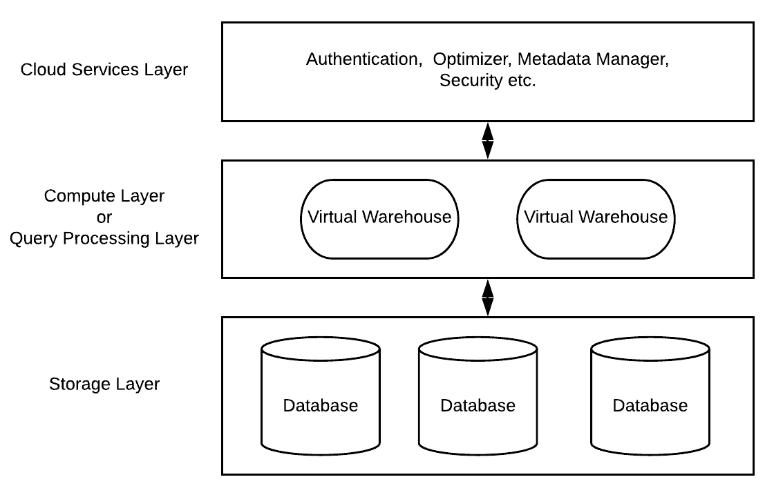
Figure 1 shows a high-level view of the Snowflake architecture.

Diagram Description automatically generated

Figure 1: Architecture of snowflake

As shown in Figure 1, the unique Snowflake architecture consists of three key layers:

Cloud Services

This is the “brain” of Snowflake where activities such as authentication, infrastructure management, metadata management, query parsing and optimization, and access control are all managed. These services tie together all the different components of Snowflake to process user requests, from login to query dispatch.

Query Processing

This layer is also known as Compute layer. Considered the “brawn” of Snowflake, the Query Processing layer performs data manipulations, transformations, and queries (data fetching) requested by users. All this processing is done by Snowflake using virtual warehouses.
Each virtual warehouse is a massively parallel processing (MPP) compute resource cluster. Each virtual warehouse consists of multiple nodes with CPU and memory automatically provisioned in the Cloud by Snowflake.

Here are some benefits of virtual warehouses:

  • Comes in different sizes from extra small to 6XL and you can change the size of an existing virtual warehouse based upon your need. When you resize your virtual warehouse, running queries remain unaffected; only new queries submitted will use the new warehouse size.
  • You only pay for the resources you utilize. If there are no workloads running, there are no costs associated with virtual warehouse compute. However, it’s important to note that you are charged for data storage regardless of usage. Can be started or stopped at any time. You can also auto-suspend, or auto-resume a Virtual Warehouse based upon a specific period of inactivity.
  • Can be set to auto-scale. This means if more queries are launched on a Virtual Warehouse, increasing the load on it, it can automatically launch new clusters to accommodate the increased load and automatically scale down when the load decreases.

Database Storage Layer

Snowflake is a columnar database. When data is loaded into Snowflake, it is internally reorganized into an optimized, compressed, columnar format. Snowflake stores this optimized data in Cloud storage. Snowflake’s database storage layer is tasked with the responsibility of storing and managing data. It utilizes a scalable and elastic storage infrastructure, effectively decoupling compute, and storage operations. The data is organized into numerous micro-partitions, optimizing data access and query performance. Notably, Snowflake’s storage layer exhibits a high level of durability, automatically replicating data across multiple availability zones to ensure reliability. Moreover, it is designed to seamlessly handle extensive data volumes and supports a wide array of data formats, enabling organizations to efficiently store and analyse diverse data types.

The internal representation of data objects is not accessible, nor is it visible, to customers. Snowflake manages all aspects of storage file organization, metadata compression, and data storage statistics. This ensures that users do not need to worry about data distribution across different micro partitions.

As the storage layer is independent, customers need to pay only for the average monthly storage used. Since Snowflake is provisioned on the Cloud, storage is elastic and is charged as per terabyte (TB) of usage per month. Compute nodes connect with the Database Storage layer to fetch data for query processing. The main benefit of columnar databases store is it stores data in columns rather than rows, they are well-suited for analytical workloads that involve querying large amounts of data. Columnar databases can retrieve data more quickly than row-oriented databases because they only need to read the columns that are required for a particular query. This can result in significant performance improvements, particularly for complex queries that involve multiple joins and aggregations.

Creating a Virtual Warehouse

Now let’s discuss how to create virtual warehouses. By default, when we create a Snowflake account it comes with a default warehouse named COMPUTE_WH. You can create new warehouses at any time using the ACCOUNTADMIN and SYSADMIN security roles in Snowflake.

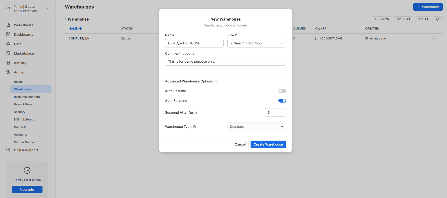
To create a new warehouse, log into the Snowflake web UI, go to the Warehouses tab and click the “+ Warehouse” button. Give your new warehouse a meaningful name. I have named my new warehouse DEMO_WAREHOUSE and kept the size as X-Small. You can also select Advanced Settings like Auto Resume and Auto Suspend from this New Warehouse dialog. Figure 2 shows the New Warehouse dialog.

Graphical user interface, application Description automatically generated

Figure 2: how to create a virtual warehouse from snowflake UI.

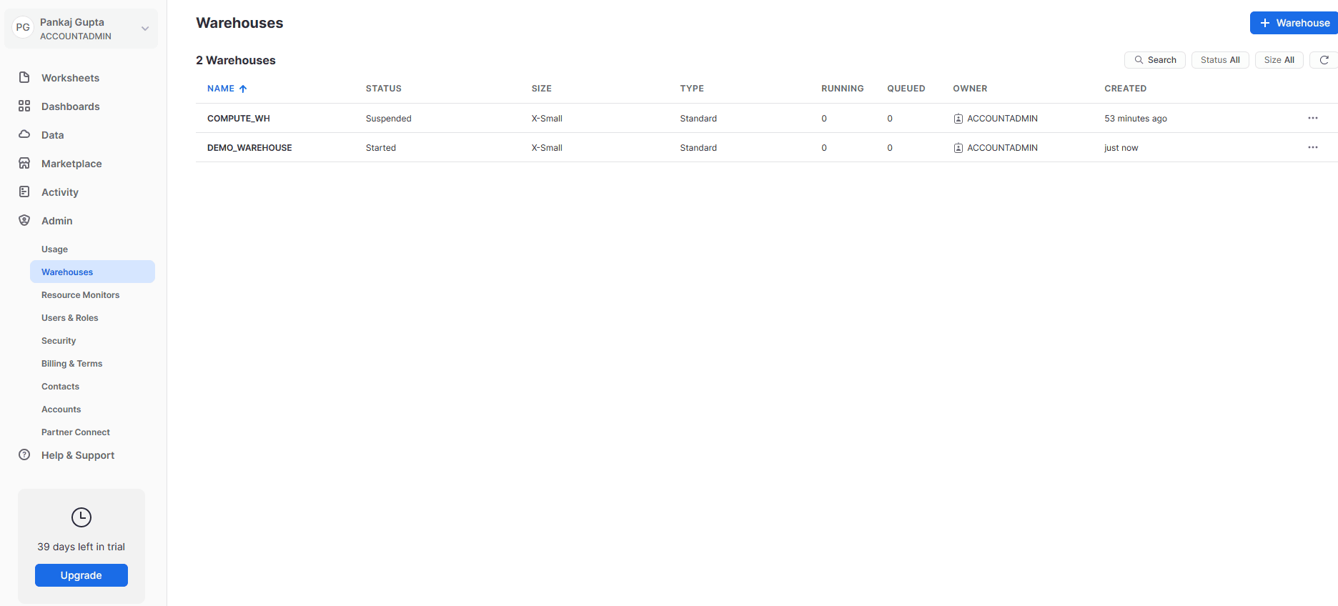
A warehouse is created within a few seconds, giving us a glimpse of the power of Cloud computing and Snowflake. We did not purchase any hardware, performed no installation, and yet we now have a data warehouse up and running within minutes. The main advantage is we can change the compute power on the fly, have multiple warehouses—like one for each department—and only pay for the resources we use. Figure 3 shows the Warehouses summary screen after we create our warehouse.

Graphical user interface, application, table, Excel Description automatically generated

Figure 3: Virtual warehouse window after creation.

You can also create warehouse using the Snowflake SQL CREATE WAREHOUSE statement, shown in Figure 4.

CREATE OR REPLACE WAREHOUSE DEMO_WAREHOUSE
WITH WAREHOUSE_SIZE = XSMALL
 COMMENT = 'This is for demo purpose only.'
  AUTO_SUSPEND = 300
  WAREHOUSE_TYPE = STANDARD;

Execute this code and you should see:

Figure 4: SQL’s and parameters for creating virtual warehouse.

You can find the full syntax and additional options related to virtual warehouse creation at the following link: https://docs.snowflake.com/en/sql-reference/sql/create-warehouse.html

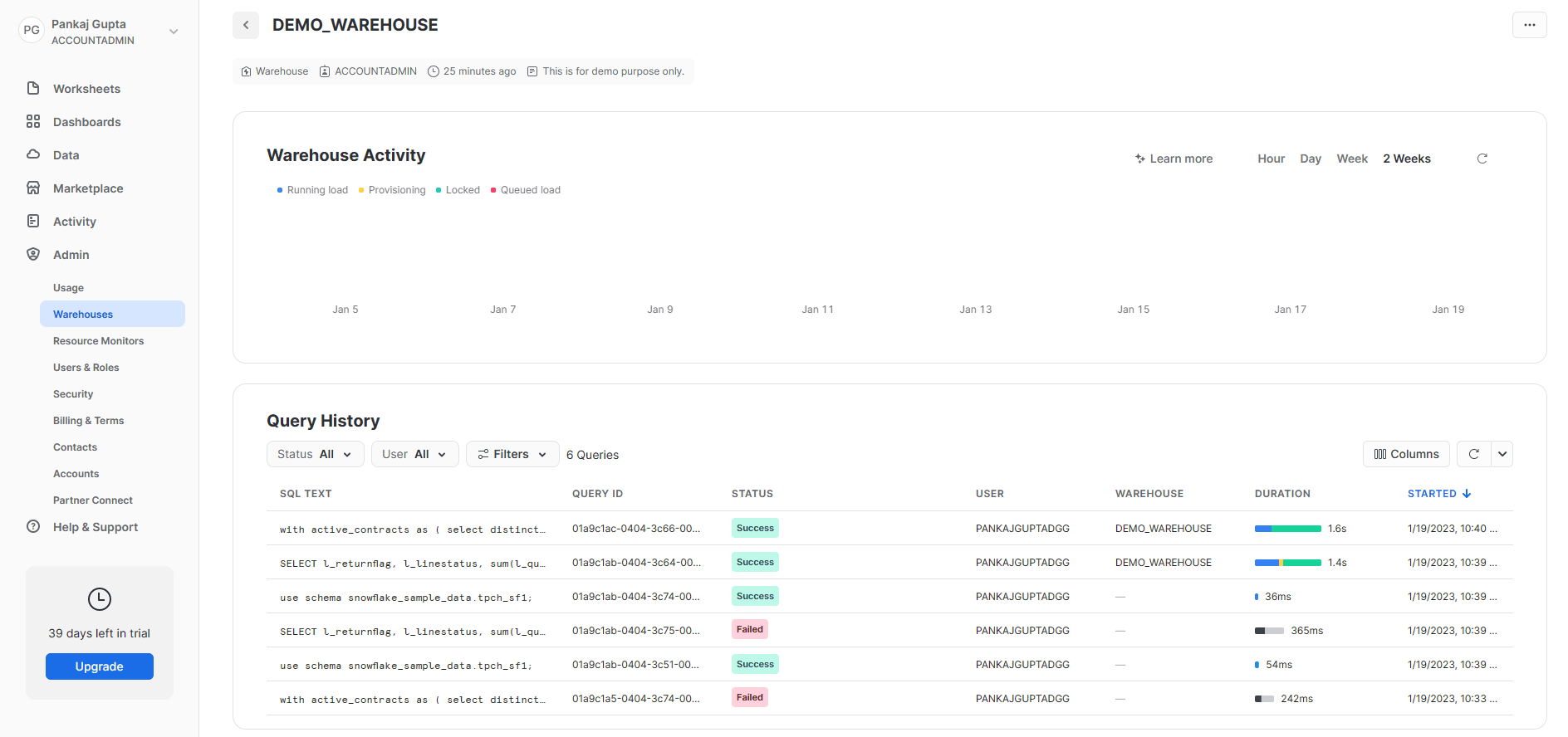
The Web UI provides access to additional features like transferring ownership, roles, and many other warehouse management functions. In the Warehouse Activity tab, you can see individual query execution metrics like executed query text, query executor, and duration, etc. Figure 5 shows the Warehouse Activity screen.

Graphical user interface, application, table Description automatically generated

Figure 5: Web UI demo for available information.

Time travel and fail safe in Snowflake:

Time travel in Snowflake enables users to retrieve historical versions of data that were previously stored in the system. This feature allows users to query the data as it appeared at a specific moment in time, regardless of any subsequent changes or deletions that may have occurred.

For more details on Snowflake time travel, see the following documentation:

https://docs.snowflake.com/en/user-guide/data-time-travel

Within the context of Snowflake, the term “fail-safe” pertains to the system’s capability to prevent data loss, corruption, or compromise in the event of a system failure or outage. The fail-safe mechanisms implemented in Snowflake are intended to uphold data integrity and to reduce the possibility of any downtimes or data loss.

For more details on Snowflake fail-safe, see the following documentation:

https://docs.snowflake.com/en/user-guide/data-failsafe

Snowflake Tables

In this section, I will cover some of characteristics of Snowflake tables to help you understand the basic architecture of how tables are built and utilized.

Table Types

Snowflake provides 3 different types of tables: Temporary, Transient, and Permanent.

Temporary Tables

Temporary tables are like permanent tables with a caveat that they only exist for the current session. A temporary table is only visible to the user who created it and cannot be accessed by anyone else. When the session ends, the data in the temporary table gets purged.

The common use case for temporary tables is storing data, which is non-permanent and can be recreated, like aggregates, etc. Temporary tables serve as a staging area for data prior to undergoing transformations or being loaded into permanent tables. They are handy for storing intermediate results during complex data processing tasks and can improve query performance by materializing intermediate results.

Figure 6 shows the creation of a temporary table.

CREATE OR REPLACE TEMPORARY TABLE DEMO_TEMP
(
NAME VARCHAR(100),
EMPLOYER VARCHAR(100),
ID NUMBER
);

Figure 6: Code for creating a temporary table.

You can find the full syntax and additional options related to create table creation at the following link: https://docs.snowflake.com/en/sql-reference/sql/create-table.

Transient Tables

Transient tables operate like permanent tables except for the fact that they do not have a fail-safe period associated with them. The maximum time travel retention period for transient tables is one day, while permanent tables in the Enterprise Edition or higher can retain data for up to 90 days. Data in the transient table is persisted until the table is explicitly dropped, so unlike a temporary table the transient table will remain even after the session it was created in ends.

There is no fail-safe cost associated with it, but it does contribute to overall storage expenses for accounts.

Figure 7 shows how to create a transient table.

CREATE OR REPLACE TRANSIENT TABLE DEMO_TEMP
(
NAME VARCHAR,
EMPLOYER VARCHAR,
ID NUMBER
);

Figure 7: Code to create a transient table.

Permanent Tables

Permanent tables have a fail-safe period and provide an additional level of data recovery and protection. A permanent table is created when data must be stored for a longer period. Permanent tables persist until explicitly dropped. Figure 8 shows the creation of a permanent table.

CREATE OR REPLACE  TABLE DEMO_PERM
(
NAME VARCHAR(100),
EMPLOYER VARCHAR(100),
ID NUMBER
);


Figure 8: Web UI creating a permanent table.

Inserting data into DEMO_PERM table:

INSERT INTO DEMO_PERM 
VALUES ('Pankaj Gupta','Test Employer','1');
INSERT INTO DEMO_PERM 
VALUES ('Ravi Jain','DataDog','2');

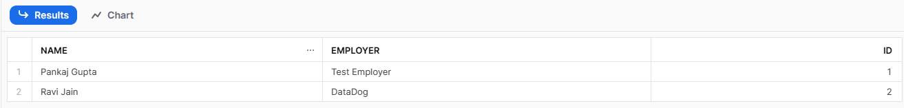
This will insert the following data as shown in Figure 9:

Figure 9: Web UI showing inserted data.

Table 1 summarizes the differences between Snowflake table types and their impact on time travel and fail-safe functionality.

Table Type

Persistence

Time Travel Retention Period (Days)

Fail-safe Period (Days)

Temporary

Remainder of session

0 or 1 (default is 1)

0

Transient

Until explicitly dropped

0 or 1 (default is 1)

0

Permanent (Standard Edition)

Until explicitly dropped

0 or 1 (default is 1)

7

Permanent (Enterprise Edition and higher)

Until explicitly dropped

0 to 90 (default is configurable)

7

Table 1. Differences Between Snowflake Table Types.

Clustering Keys and Query Performance

In this section we will consider clustering keys in Snowflake and their effect on query performance for large tables.

The clustering key in Snowflake is a designated column or set of columns that dictates the physical storage order of data within a table. It plays a crucial role in determining how data is structured and grouped together on disk, leading to notable effects on query performance and the efficiency of data retrieval. By carefully selecting the clustering key, you can optimize the organization of data on disk, resulting in improved query performance and faster access to relevant information.

A picture containing text, screenshot, number, font Description automatically generated

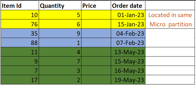
Fig. 14 shows a cluster table where data with same month in kept in same micro partitions.

Within Snowflake’s architecture, micro-partitions refer to individual units of data storage that comprise a section of a table’s data. These micro-partitions are designed to contain a relatively small amount of data, usually ranging between 50 MB to 500 MB. Moreover, data stored within each micro-partition is compressed, columnar-organized, and saved in a specialized format, which is fine-tuned to optimize query processing performance.

Clustering in snowflake relates to arrangement of rows co-located with similar rows in the same micro-partitions. The effect of clustering can be seen for very large tables (larger than 1+ TB) when ordering of data when initially loaded data was not ordered or an excessive number of Data Manipulation Language (DML) operations have been performed against the table (like INSERT, UPDATE, etc.), causing the table’s natural clustering to degrade over a period.

When a clustering key is defined on a table, the automatic clustering service will co-locate rows with similar values in their cluster key columns to the same micro-partitions.

The Benefits of Defining Clustering Keys:

  1. Better scan efficiency, making your queries execute more efficiently.
  2. Less table maintenance is required if auto-clustering is enabled, and data is not being inserted in order.
  3. Better column compression.

A clustering key can be defined on a table at the time of creation or by using the ALTER TABLE statement if the table already exists.

To demonstrate, we will create a table without any clustering key and insert data in it, using the following code. The results of this query are shown in Figure 15.

CREATE OR REPLACE TABLE DEMO_NO_CLUSTERING (
EMP_ID NUMBER(10,0),
DEPT_ID NUMBER(4,0),
EMP_NAME VARCHAR(4),
HOME_ADDR VARCHAR(1000)
);
INSERT OVERWRITE INTO DEMO_NO_CLUSTERING
SELECT
seq4() AS EMP_ID,
uniform(1, 1000, random()) AS DEPT_ID,
randstr(4, random()) AS EMP_NAME,
randstr(1000, random()) AS HOME_ADDR
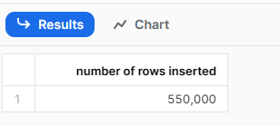
FROM table(generator(rowcount => 550000));

This will return:

A screenshot of a graph Description automatically generated with low confidence

Figure 15: Snowflake web UI showing SQL run of query.

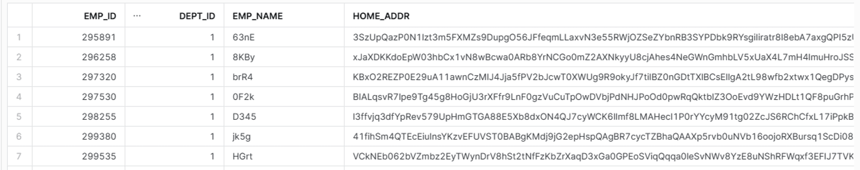
We can then select a record from our sample table using a SELECT query with a WHERE clause filter, as shown in the following code:

SELECT * 
FROM DEMO_NO_CLUSTERING 
WHERE DEPT_ID = 1;

The output is shown in Figure 16.

A screenshot of a computer Description automatically generated with low confidence

Figure 16. SELECT from sample non-clustered table.

Semi-Structured Data in Snowflake

Here we will look at the power of Snowflake’s semi-structured data handling capability. We will create a table with the VARIANT data type and use it to load semi-structured JSON data. Figure 10 shows the creation of a table with a VARIANT data type column and loading JSON data into it.

For example:

CREATE OR REPLACE   TABLE DEMO_TEMP_VARIANT
(
  LOCATION VARIANT
);

Insert below test data for loading into table.

INSERT INTO DEMO_TEMP_VARIANT 
SELECT parse_json(column1)
  from values
  ('{
    "id": "1234",
    "name": {
      "first": "Pankaj",
      "last": "Gupta"
    },
    "company": "demo_company",
    "email": "pankaj.gupta@demo_company.info",
    "phone": "+1 (123) 456-7890",
    "address": 
      "268 Havens Place, Dunbar, Rhode Island, 7725"
  }')
  , ('{
    "id": "5678",
    "name": {
      "first": "Arpan",
      "last": "Rai"
    },
    "company": "DIGIGEN",
    "email": "Arpan.Rai@DIGIGEN.net",
    "phone": "+1 (111) 222-3021",
    "address": 
     "441 Dover Street, Ada, New Mexico, 5922"
  }');

Figure 10: Running SQL and INSERT query in Snowflake web UI.

Once our JSON data has been inserted into the Snowflake table, we can view it with a SELECT query, as shown in Figure 11.

SELECT  * 
FROM DEMO_TEMP_VARIANT;

Executing this code will return:

A screenshot of a computer Description automatically generated with medium confidence

Figure 11: Showing data in Snowflake web UI.

Now we’ll consider the technique for parsing the JSON data in this table. One thing to keep in mind is that VARIANT values are not strings; VARIANT values contain strings. The operators “:” and subsequent “.” and “[]” always return VARIANT values containing strings.

Below are some pre-defined functions which can be used with variant data.

  • PARSE_JSON – pre-defined function in Snowflake that facilitates the extraction of data from strings that are formatted in JSON. This function takes a solitary parameter, which is a string that contains the data formatted as JSON, and subsequently returns a variant data type that can be used in SQL queries.
  • CHECK_JSON built-in function in Snowflake that validates whether a string contains valid JSON data. This function can be used to check if a given string is formatted correctly as JSON and returns a Boolean value of TRUE or FALSE

Sample query

SELECT CHECK_JSON( 
'
{
    "id": "1234",
    "name": {
      "first": "Pankaj",
      "last": "Gupta"
    }
  }')
as is_valid;

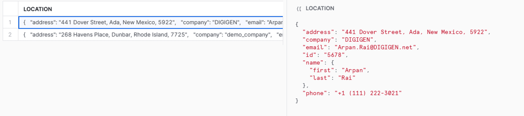
Using Snowflake’s semi-structured data extraction operators, our JSON data can simply be fetched in a flat table format using a simple query like the one shown in Figure 12.

SELECT
    (LOCATION:id) as id,
    (LOCATION:name:first) as first_name,
    (LOCATION:name:last) as last_name,
    (LOCATION:company) as company,
    (LOCATION:email) as email,
    (LOCATION:phone) as phone,
    (LOCATION:address) as address
FROM
    DEMO_TEMP_VARIANT;

Figure 12:SQL for parsing JSON in Snowflake web UI.

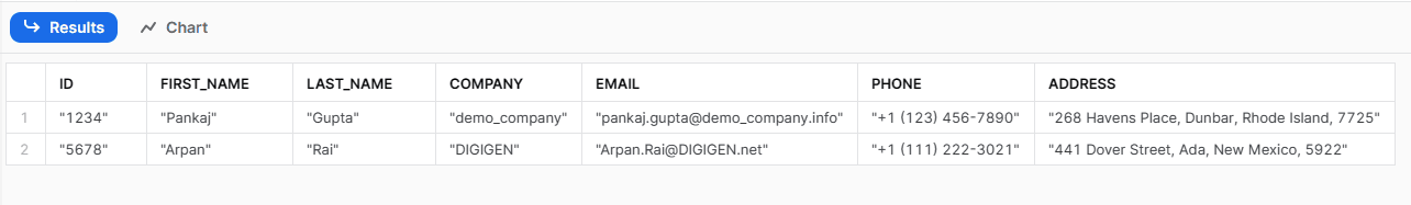
Figure 13 shows the results of our JSON extraction query.

A screenshot of a computer Description automatically generated with low confidence

Figure 13: Flattened semi structured JSON data.

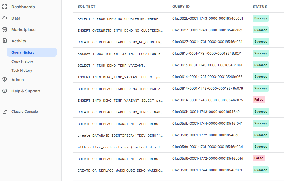
Query History and Profiling

To look as the query plan of queries that have been executed. You

can go to query profiling page through activity tab 🡪 Query History:

Graphical user interface, text, application Description automatically generated

Figure 17: query history tab

Select the query for which you want to see profile.

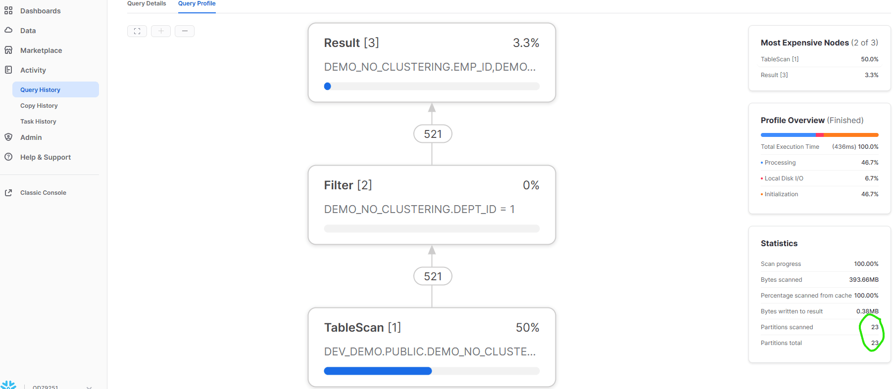
Now when we look at the query profile, we notice this table had 23 micro-partitions, and all 23 were scanned while searching for records where DEPT_ID = 1. This result is shown in Figure 18.

Graphical user interface Description automatically generated

Figure 18: Snowflake web UI showing query profile result for table with no clustering key.

Now let’s create an equivalent table with a clustering key and assess how same select query works. The query in Figure 19 creates our new table with a clustering key.

CREATE OR REPLACE TABLE DEMO_CLUSTERING 
                   cluster by (DEPT_ID) (
EMP_ID NUMBER(10,0),
DEPT_ID NUMBER(4,0),
EMP_NAME VARCHAR(4),
HOME_ADDR VARCHAR(1000)
);
    
INSERT OVERWRITE INTO DEMO_CLUSTERING
SELECT
seq4() AS EMP_ID,
uniform(1, 1000, random()) AS DEPT_ID,
randstr(4, random()) AS EMP_NAME,
randstr(1000, random()) AS HOME_ADDR
FROM table(generator(rowcount => 550000)) 
ORDER BY DEPT_ID;

Figure 19: DDL and SQL for execution in snowflake web UI

Now run the equivalent SELECT query from our previous example against the new table, as shown.


SELECT *
FROM DEMO_CLUSTERING
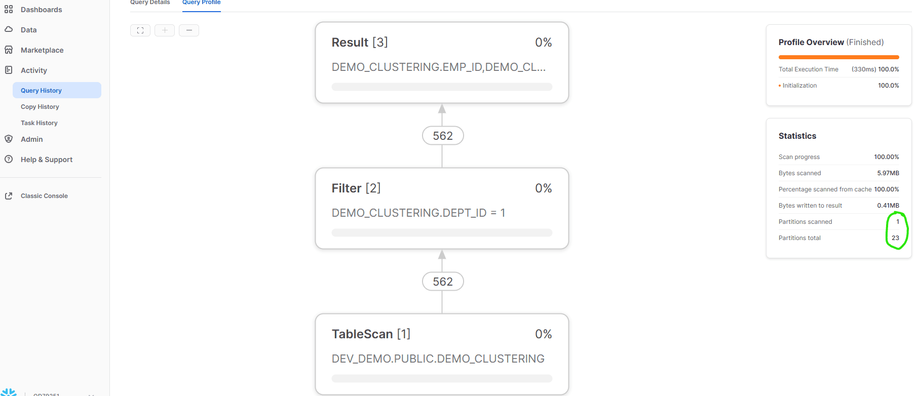
WHERE DEPT_ID = 1;

When we look at the query profile, we can clearly see that with a clustering key enabled on the DEPT_ID column, this query scans only 1 partition of the 23 available. If there are thousands of partitions, then clustering key can increase CPU resource efficiency and result in more efficient execution. The key thing here is that data should be inserted for the clustering key in the sorted order in our table. This is why we apply the ORDER BY clause to the SELECT query that feeds our INSERT statement. If you do not load data in sorted order for DEPT_ID, it will not organize micro-partitions properly and will still scan all the micro-partitions. Figure 20 shows our query profile after applying a clustering key and inserting our data into the table in clustering key order.

Graphical user interface Description automatically generated

Figure 20: Snowflake web UI showing query profile result for table with clustering key.

Within most traditional database management systems (DBMSs), utilization of the ORDER BY clause within a SELECT query that feeds a DML statement, such as UPDATE or DELETE, does not inevitably guarantee ordering of the resulting data. Consequently, rows retrieved by such a query might not consistently maintain the same order every time the query is executed, even if the ORDER BY clause is used.

Nevertheless, this characteristic distinguishes Snowflake from most other DBMSs. When using Snowflake, the ORDER BY clause in a SELECT query that feeds a DML statement does guarantee ordering of the resulting data. Hence, rows returned by the query will persistently maintain the same order, regardless of how many times the query is executed.

This guarantee of ordering can be attributed to Snowflake’s unique architecture. Its micro-partitioning technique and query optimization methods permit highly efficient and parallelized query execution, resulting in ordered outputs even when using the ORDER BY clause in a DML statement.

Summary

In this article we considered the basic differences between an on-premises infrastructure and a Cloud-based infrastructure. We then discussed the Snowflake architecture and created a new virtual warehouse. We discussed the different types of tables Snowflake supports and created each type of table. We also covered how to load semi-structured data in Snowflake in a VARIANT data type column, and how to extract JSON data in a tabular format. Finally, we discussed clustering keys and performed a practical demonstration that showed the difference between tables created with and without a clustering key.

References

Snowflake Documentation: https://docs.snowflake.com/en/

Here are a few popular Cloud providers you can visit to get additional information. There are many more, and this article does not endorse any specific one. The links are for informational purposes only.

Amazon Web Services: https://aws.amazon.com/

Microsoft Azure: Cloud Computing Services | Microsoft Azure

Google Cloud Platform: Cloud Computing Services | Google Cloud


The post Snowflake: A Cloud Warehouse Solution for Analytics appeared first on Simple Talk.


from Simple Talk https://ift.tt/0vnfIeK
via