Monday, July 31, 2023

Running Queries Across Many SQL Server Databases

A challenge that reappears periodically in the world of databases (especially database management) is the need to run code on a subset of databases and to do so in a nuanced manner. Some maintenance or metrics collection processes can be simply run against every database on a server with no ill-effect, but others may be app-specific, or need to omit specific sets of databases.

This article dives into how to create and customize your own solution, tackling everything from filtering databases to validating schema elements to error-handling.

What About sp_MSforeachdb?

The sp_MSforeachdb system stored procedure can be used to run T-SQL across many SQL Server databases. While that sounds ideal, it is an undocumented black box that does not always perform the way you may want it to. Undocumented features can be used with extreme caution, but it is inadvisable to make them a key part of important processes as they may change, be deprecated, or be discontinued with little or no notice.

In addition, sp_MSforeachdb has no ability to be customized or expanded upon. What you see is what you get and there is no flexibility if it does not do precisely what you want.

This article covers some of the things done in a procedure named dbo.RunQueryAcrossDatabases that you can download in a .zip file: RunQueryAcrossDatabases_FullScript.

Code Reusability

The common solution to this problem is to create new code that iterates through databases for each application or process whenever it is needed. While this certainly is functional, it poses all of challenges of code maintainability when the same code is copied into many places.

If a new database appears that is an exception the rules, then each and every process would need to be inspected and adjusted as needed to ensure that the exception is accounted for. Even on a small number of database servers, it is likely that one might be omitted and cause unexpected (and perhaps, not quickly noticed) harm. If hundreds of servers are being maintained, then the odds of missed many become quite high.

A single universal stored procedure that is used for this purpose ensures that when changes are needed, they can be made a single time only:

  • Update the stored proc in source control.
  • Test it in dev/QA.
  • Deploy to production.

Because this process follows the typical one used for deploying application-related code, it is familiar and less likely to result in mistakes or omissions. In addition, a solution that is parameterized can ensure that when changes are needed, they can be made to parameter values and not to source code, minimizing the need for more impactful changes.

Building a Code Execution Solution

To build a solution that executes T-SQL for us, there is value in listing the steps needed to accomplish this task:

  • Create and apply filters to determine which databases should have code executed against them.
  • Create code that will run against that database list.
  • Iterate through that database list.
  • Run the code against each of those databases.

When written out as a list, it becomes clear that this task is far simpler than it sounds, which means that our job of writing this code can move quickly through the necessities and into customization (which is far more fun!)

Note that a complete/working solution is attached at the end of this article. Feel free to download and customize it to your heart’s content!

Create and Customize a Database List

The key to this process is to create a list of databases that code will be run against. This may be as simple as an explicit list of N databases, but more often than not will involve some more detailed logic. For example, there may be a need to filter out all databases that do not meet a specific naming convention. Alternatively we may want to exclude databases by name.

Ultimately, this entire task comes down to querying sys.databases and filtering based on information in the system view. Yeah, you heard that right: SELECT from a view and add a WHERE clause and DONE! OK, it isn’t quite that simple, but we’ll do our best to not make this complex. In order to create this process, dynamic T-SQL will be used. It is possible to do this via standard SQL by creating/modifying a database list step-by-step, adding and removing databases along the way. While this certainly works, I find the resulting code even more convoluted than dynamic SQL (yes, I said that!).

As a brief reminder, sys.databases is a system catalog view that provides a row per database on the server. Included in that data is a hefty amount of metadata and operational information that tells us how a database is configured and its current state. The following query returns some basic (but useful) information from this view:

SELECT
        databases.name,
        databases.database_id,
        databases.create_date,
        databases.compatibility_level,
        databases.collation_name,
        databases.user_access_desc,
        databases.state_desc,
        databases.recovery_model_desc
FROM sys.databases;

The results provide a whole lot of actionable info:

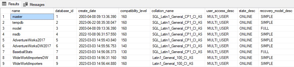
When inspecting databases, knowing the compatibility level, collation, or current state could be critical to making decisions about whether or not to query them and especially apply changes to them. At a higher level, there is value in knowing this information regardless. For example, that BaseballStats database of mine…should that really be set to compatibility level 130 (SQL Server 2016)?! If that were an oversight, then it can be corrected. Similarly, should only two databases be using the FULL recovery model? Another fine question for an administrator/operator to consider.

Note that the database list above will be used for the duration of this article. The databases on your test server, as well as related objects and metadata will vary from what is presented here.

To start, let’s limit the database filtering to database name only. Additional customization based on other details is relatively easy to add once a starter-query has been constructed. To do this, a handful of variables will be introduced:

DECLARE @DatabaseNameLike VARCHAR(100) = 'WideWorldImporters';
DECLARE @DatabaseNameNotLike VARCHAR(100);
DECLARE @DatabaseNameEquals VARCHAR(100);

These filters can be added one by one as filters to sys.databases. If any filter is NULL, it can be ignored:

SELECT
        *
FROM sys.databases
WHERE (@DatabaseNameLike IS NULL 
       OR name LIKE '%' + @DatabaseNameLike + '%')
AND (@DatabaseNameNotLike IS NULL 
       OR name NOT LIKE '%' + @DatabaseNameNotLike + '%')
AND (@DatabaseNameEquals IS NULL OR name = @DatabaseNameEquals);

If @DatabaseNameLike is set to 'WideWorldImporters' and the other variables are left NULL, then the results of the above query would return:

There are no limits to filtering like this. It would be relatively easy to add additional filters for names that start with a prefix, end in a suffix, or any other comparison that can be dreamed up.

Another common need is to omit system databases from queries. Running some T-SQL across many databases may include model, master, tempdb, and msdb, but oftentimes will not. This added filter to the query above can be handled by another variable and one more WHERE clause:

DECLARE @DatabaseNameLike VARCHAR(100) = 'WideWorldImporters';
DECLARE @DatabaseNameNotLike VARCHAR(100);
DECLARE @DatabaseNameEquals VARCHAR(100);
DECLARE @SystemDatabases BIT = 0;
SELECT
        *
FROM sys.databases
WHERE (@DatabaseNameLike IS NULL 
     OR name LIKE '%' + @DatabaseNameLike + '%')
AND (@DatabaseNameNotLike IS NULL 
     OR name NOT LIKE '%' + @DatabaseNameNotLike + '%')
AND (@DatabaseNameEquals IS NULL 
     OR name = @DatabaseNameEquals)
AND (@SystemDatabases = 1 
     OR name NOT IN ('master', 'model', 'msdb', 'tempdb'));

If a search is run using @DatabaseNameLike = 'B' and @SystemDatabases = 1, then the results will look like this:

If the same search is performed, but with @SystemDatabases = 0, then the results are reduced to only a single result:

Sys.databases contains quite a few columns that can be filtered as easily as the name, such as compatibility level, collation name, user access (is it in single or multi-user?), state, recovery model, and much more. Adding filters can be accomplished on any column in the same fashion as above. For example, if there is a need to query all databases on a server – but only those that are online and multi-user, the query above could be adjusted as follows:

DECLARE @DatabaseNameLike VARCHAR(100) = 'WideWorldImporters';
DECLARE @DatabaseNameNotLike VARCHAR(100);
DECLARE @DatabaseNameEquals VARCHAR(100);
DECLARE @SystemDatabases BIT = 0;
DECLARE @CheckOnline BIT = 1;
DECLARE @CheckMultiUser BIT = 1;
SELECT
        *
FROM sys.databases
WHERE (@DatabaseNameLike IS NULL 
       OR name LIKE '%' + @DatabaseNameLike + '%')
  AND (@DatabaseNameNotLike IS NULL 
       OR name NOT LIKE '%' + @DatabaseNameNotLike + '%')
AND (@DatabaseNameEquals IS NULL 
     OR name = @DatabaseNameEquals)
AND (@SystemDatabases = 1 
     OR name NOT IN ('master', 'model', 'msdb', 'tempdb'))
AND (@CheckOnline = 0 
      OR state_desc = 'ONLINE')
AND (@CheckMultiUser = 0 
      OR user_access_desc = 'MULTI_USER');

Run this query, and you will get back WideWorldImportersDW and WideWorldImporters. To test the offline change, let’s set WideWorldImportersDW offline:

ALTER DATABASE WideWorldImportersDW SET OFFLINE;

If you want to make it happen immediately on your local machine, you can add: WITH NO_WAIT ROLLBACK IMMEDIATE; and it will kill existing transactions/connections and apply the ALTER DATABASE command.

Now, run the query and the offline database is removed from the results:

We’ve dove into filtering the database list by metadata in sys.databases. Next up is how to filter based on the existence (or non-existence) of objects.

Validating the Presence of Objects

Another common challenge when executing a query across any number of databases is to only run the query if a specific table or object exists. Some examples of this include:

  • Select data from a table, but only if it exists (or if a specific column in that table exists).
  • Execute a stored procedure, but only if it exists. This prevents throwing “Object Not Found” errors.
  • Validate if an object exists and log details about it, depending on its status.
  • Check if a release completed successfully.

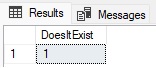
At its core, this is not a challenging task. There are many views available in SQL Server that allow us to check and see if an object exists or not. For example, the following code will check if the table Sales.Customers exists in the WideWorldImporters database:

SELECT
      COUNT(*) AS DoesItExist
FROM WideWorldImporters.sys.tables
INNER JOIN WideWorldImporters.sys.schemas
ON tables.schema_id = schemas.schema_id
WHERE tables.name = 'Customers'
AND schemas.name = 'Sales';

The result is straightforward, since there is one table name Sales.Customers in the WideWorldImporters database:

What I want is for the logic behind this to be encapsulated into the process we are building. Having to rewrite this code every single time an object needs to be checked for is cumbersome, and someone will eventually make a mistake.

To get us started, two new parameters will be declared:

DECLARE @SchemaMustContainThisObject VARCHAR(100);
DECLARE @SchemaCannotContainThisObject VARCHAR(100);

When @SchemaMustContainThisObject contains a value, then its presence will be validated and only databases that contain it will have the query executed against them. When @SchemaCannotContainThisObject contains a value, then databases that contain that object will be excluded.

The following is a simple implementation of this logic, looking for the number of schemas that have a Customers table in the WideWorldImporters database:

DECLARE @SchemaMustContainThisObject VARCHAR(100) = 'Customers';
DECLARE @SchemaCannotContainThisObject VARCHAR(100);
DECLARE @DatabaseName sysname = 'WideWorldImporters'
DECLARE @SQL NVARCHAR(MAX);
DECLARE @ObjectValidationCount INT;
DECLARE @ObjectExceptionCount INT;
DECLARE @ParameterList NVARCHAR(MAX);
IF @SchemaMustContainThisObject IS NOT NULL
BEGIN
     SELECT @SQL = 'SELECT @ObjectValidationCount = COUNT(*) FROM ' + 
               QUOTENAME(@DatabaseName) + --in case database name has 
                                          --spaces/special characters
                  '.sys.objects WHERE objects.name = ''' +  
               @SchemaMustContainThisObject + ''';';
     SELECT @ParameterList = '@ObjectValidationCount INT OUTPUT';
     EXEC sp_executesql @SQL, 
                        @ParameterList, 
                        @ObjectValidationCount OUTPUT;
END;
IF @SchemaCannotContainThisObject IS NOT NULL
BEGIN
     SELECT @SQL = 'SELECT @ObjectExceptionCount = COUNT(*) FROM ' + 
            QUOTENAME(@DatabaseName) + 
            '.sys.objects WHERE objects.name = ''' + 
            @SchemaCannotContainThisObject + ''';';
     SELECT @ParameterList = '@ObjectExceptionCount INT OUTPUT';
     EXEC sp_executesql @SQL, 
                        @ParameterList, 
                        @ObjectExceptionCount OUTPUT;
END;
SELECT @ObjectValidationCount AS FoundObjectCount,
       @ObjectExceptionCount AS NotFoundObjectCount;

Executing this code, you will see that there are two schemas in the WideWorldImporters have a Customers object (the one we have been working with, and another a view object in the Website schema).

Additional variables are declared to support parameterized dynamic SQL, as well as to store the output of the test queries. The counts can then be checked later to validate if an object exists or not. Note that sys.objects is used here for convenience without any added object type checks. If additional criteria or object types need to be checked, adding checks on the type_desc column in sys.objects can be used to further filter object details and return exactly what you are looking for. If only tables are checked, then sys.tables could be used instead. Similarly, if there is a need to check multiple types at once, additional variables/parameters could be declared for different object types.

Providing an Explicit Database List

A simple, but common implementation of this is to have an added parameter that provides an explicit database list to run a query against. If it is known exactly which databases need to be executed against and the list will not change without this code being altered, then it is possible to pass in a detailed list. This can be accomplished with a string or table-valued parameter, depending on your preference. Since the number of databases (and the length of this list) is bound by how many databases you have in a single place, it’s not likely that the length of this list would become prohibitively long for either solution. Therefore, the database list may be stored as a comma-separated-values string, like this:

DECLARE @DatabaseList VARCHAR(MAX);
SELECT @DatabaseList = 
          'AdventureWorks2017, BaseballStats, WideWorldImporters';

It may also be stored using a table-valued parameter:

CREATE TYPE dbo.DatabaseListType AS TABLE
     (DatabaseName SYSNAME);
GO
DECLARE @DatabaseList dbo.DatabaseListType;

Similarly, the table variable may be memory-optimized, if your SQL Server version supports it and you are so inclined:

CREATE TYPE dbo.DatabaseListType AS TABLE
     (DatabaseName SYSNAME PRIMARY KEY NONCLUSTERED)
WITH (MEMORY_OPTIMIZED = ON);
GO
DECLARE @DatabaseList dbo.DatabaseListType;

If you choose that option, it is also worth considering using natively compiled stored procedures for consuming memory-optimized table variable. This is not an article about memory-optimized-awesomeness, and therefore a discussion of that will be skipped here. In either case, database names can be inserted into the user-defined table type like this:

INSERT INTO @DatabaseList
        (DatabaseName)
VALUES
     ('AdventureWorks2017'),
     ('BaseballStats'),
     ('WideWorldImporters');

The final step is to prepare the T-SQL to execute and run it against the selected database list. A loop will be used to iterate through each database to run against. Assuming the query to execute is stored in the variable/parameter @SQLCommand, and the name of the current database to execute against is stored in @DatabaseName, then the resulting execution code would look like this:

CREATE TABLE #DatabaseList
        (DatabaseName SYSNAME,
         IsProcessed BIT);
INSERT INTO #DatabaseList
        (DatabaseName, IsProcessed)
--<<<[Database List Determined Above and 0 for IsProcessed]>>>
DECLARE @CurrentDatabaseName SYSNAME,
        @SQLCommand nvarchar(max);
WHILE EXISTS (SELECT * FROM #DatabaseList WHERE IsProcessed = 0)
BEGIN
        SELECT TOP 1
                @CurrentDatabaseName = DatabaseName
        FROM #DatabaseList
        WHERE IsProcessed = 0;
                            -- Replace "?" with the database name
        SELECT @SQLCommand = REPLACE(@SQLCommand, 
                                      '?', @CurrentDatabaseName); 
                           
        EXEC sp_executesql @SQLCommand;
        UPDATE #DatabaseList
                SET IsProcessed = 1
        WHERE DatabaseName = @CurrentDatabaseName;
END;
SELECT *
FROM   #DatabaseList;

Executing this code using the table variable created earlier in the section, you will see that the databases you passed in will be processed (in this snippet of code, it will actually work whether the database exists or not)

There are many ways to write this code, so if your own implementation varies from this and works, then roll with it 😊 The only added feature in there is to replace question marks with the database name. Note that if your query naturally contains question marks, then this may be problematic. This was added to mimic the behavior of sp_msforeachdb and make it easy to insert/use the local database name for each database that is executed against in the loop. If your environment makes common use of question marks in code, then feel free to adjust it to a character or string that is more obscure/deliberate.

Conclusion

Building reusable tools is fun and can provide a great deal of utility in the future if more needs arise that require code like this. A script containing all elements in this article is attached. Feel free to use it, customize it, and provide feedback if you think of new or interesting ways to tweak it.

There is value in avoiding use of undocumented SQL Server features in production environments. Fortunately for this tool, replacing it is not very complicated, and the new version can be given significantly more utility!

The post Running Queries Across Many SQL Server Databases appeared first on Simple Talk.


from Simple Talk https://ift.tt/JMPCYqi
via

Unmasking SQL Server Dynamic Data Masking, Part 5, Mitigations and Summary

This is the fifth and final part of this series on SQL Server Dynamic Data Masking. The first part in the series was a brief introduction to dynamic data masking, completing solutions, and use cases. The second part covered setting up masking and some examples. The third and fourth sections explored side channel attacks against dynamic data masking.

This final part covers mitigations to side channel attacks, additional architectural considerations and an analysis of the overall solution.

Side Channel Attack Mitigations

Now that the reality of side-channel attacks is clear, mitigations for attacks need to be explored. The main foundation of mitigations is that data can’t be attacked if it is not accessible. As shown in previous examples, the attack vector for masked data starts with authorization. The functional nature of masked data, including joins, functions and clauses, requires vulnerability to these side channel attacks. All of the strengths and uses of masked data rely on the data being accessible at some level. If a user is not authorized for the data, they don’t have a foothold to attack the data. A smaller footprint also helps mitigate damage from compromised accounts, as the bad actor will have access to less data and hopefully fewer systems. This is all a pillar of the principle of least privilege.

Rely on your regular user audits and authorization mechanisms to provide access to the data. Only trusted users should be allowed access to data. Even if that data is masked. Most users won’t be savvy enough to unmask the data, but if they get a foothold into the database they will be able to peek under the covers. Data security happens in many layers. It starts with trust. If you don’t trust your users, they shouldn’t have direct access to the data. If they don’t have direct access to the data it is not possible for the users to unmask the data.

Limit Users

The primary defense against side channel attacks is limiting users that have access to your data to those that are trusted. This is clear and straight forward, part of standard security practices. Business users and even business owners don’t always understand the implications of bad security practices, they just want the project to work. You have to be a technical ambassador for the project and for security.

It is very easy to apply the db_datareader built in role to all users but it may not be the best strategy. Security design should be at the forefront of database design, from schema creation, group access, and advanced features like dynamic data masking and RLS. Carefully consider how objects will be accessed during the design phase of the database and project. If you use staging tables or there are pre-processed report tables, remember security on these objects. Pre-processing and staging data is often best done in a separate database. Regular users shouldn’t have access to this database, simplifying the security model.

Another important reminder is that data isn’t masked for from system administrators (sa login/ sysadmin role). You can audit those users and you can lock them down in other ways, such as Row-Level Security (RLS), but the nature of the super-powered roles means there is always a workaround. The workaround can be as simple as assigning security or granting access to additional objects in RLS by performing an insert statement. There is no substitute to trusting your administrators. If an administrator is a bad actor, it is much more difficult to limit damage.

No matter how data is locked down, administrators can always restore a copy to an unmanaged instance and make security changes in that instance that includes no logging. There is also the option of using DBCC PAGE to directly examine data in data files and log files, which could be done directly against a production database.

Locking Down Users

The mitigations discussed assume that the rest of your network is hardened, and users already have to pass through multiple layers to reach your databases. Establishing a good working relationship with the networking and firewall teams is critical to ensuring your database is safe. As previously mentioned, you must also work with the business to determine how the data should be protected. Security is a compromise.

The most secure data is locked in a room and is not accessible by anyone over the network, but that isn’t very usable. Security depends on layers. Procedural, physical, network, active directory, server, database, row level, schema level, etc. One layer of security, including dynamic data masking isn’t sufficient. Each layer works best when it is as transparent as possible and non-intrusive to the end users. When security breaks the flow of work it is less likely to be used. Dynamic data masking is non-intrusive and easy to implement so it meets that criteria. Each layer of security in your solution should meet that same criterion.

Architectural Decisions

Fundamental design decisions impact the data that is potentially exposed via side channel attacks. In additional to user selection and security design, the table architecture and columns configured is a foundational part of limiting exposure. As seen in the proof-of-concept scripts above, it is possible for data to be unmasked.

If exposing sensitive financial data, or any numeric data, it would be more secure rolled up into categories rather than giving access to individual rows. This is a good practice for multiple reasons, in addition to security considerations. Performance, data storage, repeatability are all improved by pre-aggregating the data. If drilldowns to the transaction level data is necessary, consider leaving out the masked column data for those details.

Masking isn’t a good solution for transactional databases and should be used with caution on non-aggregated data. Masking should be used on data that doesn’t expose proprietary business attributes or personally identifiable information. SOX compliant, HIPAA compliant, GDPR compliant, and other systems that must comply with a regulatory body, should use masking carefully and only as part of an architectural design that ensures the security of the data. These systems are typically audited, but that should be verified and implemented if they aren’t currently audited. Also be sure to work with the network and security teams to be sure they are aware of the sensitive nature of the data so they can also monitor for suspicious traffic.

Encryption

Another layer of security to be considered is encryption. Encryption also is available in layers, but doesn’t have to be implemented at each layer. TLS / SSL (on the wire encryption), at rest encryption (detached database files), backup file encryption, column level encryption (many options for this including database key level encryption), client implemented encryption, etc.

Given the nature of most types of encryption in SQL Server, it doesn’t protect against unauthorized unmasking of data. If data is encrypted at a per-client or per-user level, it would protect between clients, but not data within their scope. If data is directly accessible to end users in an unencrypted state, no matter how it is masked, it is potentially vulnerable. It is a matter of priority for a bad actor.

Data that is only unmasked in the client application can still be captured via screenshots. If that is somehow disabled by the administration team, it could still be captured by taking a picture of the screen. There is always a work-around. The principle of least privilege should always be used. And it is always harder to remove access than to grant access. This is true for service accounts as well as user accounts. Removing access after a project / database has been deployed requires regression testing and a thorough understanding of the application. In larger or complex projects, this isn’t a simple matter.

 Monitoring and Audits

Data access should be monitored and regularly audited. Most organizations of size have hundreds if not thousands of databases. It is not possible to constantly monitor these databases manually, custom scripts and audits must be used to make this feasible. Extended events focusing on excessive access to masked columns can be used to find potential unmasking activity. Auditing users with access to unmasked data should also be a common practice. It can be difficult to monitor security configurations on large teams, especially when approvers are not extremely technical.

Verifying that security hasn’t changed and is implemented as expected is an important audit activity. DBA and monitoring tasks are often handled by a different team than the team creating the masking solution. As described above, dynamic data masking requires deep understanding of the project and business rules, which is not possible for DBA teams managing hundreds of servers. It is essential for the teams to work together, especially on systems with sensitive data.

Built in protections / mitigations

In this section, I will outline a couple of the built in protections against invalid data use.

Copying the data out to another table has no impact

If masked data is copied to a new table or extracted, the masking is maintained. This alleviates some concerns about masking and supports the basic functionality of masking. This means that the new table or extract data will have the unmasked data represented as unmasked data, and the masked data will be shown with the same mask as seen in SSMS. The copied data loses the functionality of native masking but preserves the security. If data is extracted via a report, BCP, SSMS, or any other query tool, the masking status is maintained.

If data is put into a new table with a SELECT INTO, masking is maintained. This leaves the primary concern as setting up security correctly and monitoring for any possible breaches. This also questions the basic premise of masking data. If users shouldn’t be allowed to see data in an unmasked stated, why give them access in any form? It is easy, it does not impact existing functionality, and it can be used in any future functionality.

Copying to memory optimized table has no impact. Extractions do not unmask data.

Memory optimized tables and other advanced features have no impact on masking. If data is moved from the masked table to another table or an extract file, the mask is now the actual data. The same is true if the data is moved to a temp table, table variable, or a memory optimized table. If a data column is masked and is then exported, the export will contain your mask. For example, if the default mask was used for a date, all export rows will contain the value 1900-01-01 00:00:00.0000000. This means that mitigations aren’t needed for extracts, inserts, updates or any other standard data movements and manipulations.

System maintained temporal tables (history tables) are another way to potentially access unmasked data. The history table associated with each base table has a copy of each row as it changes in the base table. When a column in the base table is masked, the associated column in the history table is also masked. This table is vulnerable to the same types of side channel attacks but is not vulnerable directly.

Summary and Analysis

It might work best to finalize the discussion of dynamic data masking by describing both what it is and what it is not. Starting with the positives, data masking implements a form of obfuscation. The data is not actually changed rather it is scrambled as it is presented from the data engine. This allows the data engine to perform all of the normal operations on the data with no modifications to queries, including functions and matching in WHERE or ON statements. Because the data is not actually modified it also makes it transparent to existing queries. Data masking is a customizable masking solution built into the engine. This allows the data and the type of obfuscation to be determined by the development team. Data masking is also part of a layered approach to security. It is not a replacement for other security mechanisms, but it is a complementary layer to your current security.

There are potential gaps in the security and it can’t be the only method of making data safe, but it helps. It is also safe at a presentation layer. If used in reports it can be extremely secure. The converse side of that is the database engine level. It is a potential risk if users are allowed direct access to data in the engine. Be sure you know the weaknesses and monitor your database carefully if users are allowed to access databases directly.

The positive list for dynamic data masking makes some of the items on the negatives obvious. It is not encryption. Don’t expect the data to be 100% secure if users have direct access. The obfuscation has some weaknesses that could be exploited by a savvy user. Since it is a possible layer of security, it is not a replacement for other security mechanisms. All security should be implemented as in any other project. And even though it is a layer in a security solution, it is not a traditional security mechanism. Users will still be able to query data that is masked and join to it. There are multiple ways to take advantage of these functional parts of the solution. Another reminder is that dynamic masking is not column level security. Users are still able to query the column, they just get obfuscated data.

Dynamic data masking can be a useful part of a business intelligence solution. Understanding the limitations, strengths, and mitigations to dynamic data masking is an important part of implementing a solution. It’s also important to remember that this is a single part of a security strategy. Security works in layers and this is no exception.

This analysis isn’t meant to castigate Microsoft and their implementation of data masking. To fit existing queries and business requirements, it is a good blend of security and compromise. It is also a good reminder that direct query access and data extracts should only be available to trusted users and partners. There is often a work-around for security protocols if direct access is granted to data. Data security is very similar to physical security and hardware. If you can touch the machine, there is usually a way into it. If you have direct access to the data and enough time, there is usually a way to the base data. Be careful, use multiple layers of defense, and monitor your database activity. Dynamic data masking isn’t a magic bullet to security, but it is a potential layer to help secure data. Each layer should be monitored and each layer should be audited regularly.


The post Unmasking SQL Server Dynamic Data Masking, Part 5, Mitigations and Summary appeared first on Simple Talk.


from Simple Talk https://ift.tt/aSVxe20
via

Thursday, July 27, 2023

Exporting data from a MySQL database using SELECT…INTO OUTFILE

This article is part of Robert Sheldon's continuing series on Learning MySQL. To see all of the items in the series, click here.

In the previous article in this series, I introduced you to the MySQL LOAD DATA statement, which lets you retrieve data from a plain text file and insert it into a table. In this article, I cover the SELECT…INTO OUTFILE statement, a type of SELECT statement that includes the INTO OUTFILE clause. The clause lets you export data from one or more MySQL tables into a plain text file, providing a counterpart to the LOAD DATA statement.

Building a SELECT…INTO OUTFILE statement is relatively straightforward. The main part of the SELECT statement (without the INTO OUTFILE clause) is like any other SELECT statements, except for a couple minor considerations. And the INTO OUTFILE clause itself is fairly easy to construct. Perhaps the biggest issue you’ll run into is not having the permissions necessary to save a file to the target folder, which I discuss later in the article. Otherwise, you should have little problem getting started with the INTO OUTFILE clause.

In this article, I show you multiple examples that demonstrate how the clause works so you have a foundation in how to use it to export data. Most of the examples are built with basic SELECT statements, so they should be fairly easy for you to try out. If you have any questions about the SELECT statement itself (other than the INTO OUTFILE clause), refer to an earlier article in this series that introduces you to the statement.

Note: The examples in this article are based on a local instance of MySQL that hosts a very simple database and tables. The last section of the article—“Appendix: Preparing your MySQL environment”—provides information about how I set up my system and includes the SQL script for creating the database and tables on which the examples are based.

Introducing the SELECT…INTO OUTFILE statement

Before we jump into the examples, you should have a basic understanding of the INTO OUTFILE clause and how it fits into a SELECT statement. The following syntax shows the elements that make up the clause:

SELECT statement_elements
INTO OUTFILE 'file_name'
[FIELDS
  [TERMINATED BY 'string']
  [[OPTIONALLY] ENCLOSED BY 'char']
  [ESCAPED BY 'char']]
[LINES
  [STARTING BY 'string']
  [TERMINATED BY 'string']];

The SELECT statement itself is shown only with statement_elements placeholder, which represents all the elements that can potentially be included in a SELECT statement, other than the INTO OUTFILE clause. For the most part, you can create just about any type of SELECT statement. The main caveat is that you should not use an INTO OUTFILE clause in a nested SELECT statement because that statement must return its results to the outer statement.

The MySQL documentation also states that MySQL places “constraints on the use of INTO within UNION statements.” Unfortunately, the documentation does not state what those constraints might be. I was able to run a UNION statement that included an INTO OUTFILE clause tagged onto the end of the statement, and it created the file just fine. However, when I placed the clause just before the first FROM clause, I received an error stating that the INTO clause must be placed at the end of the UNION statement, so perhaps “constraints” applies primarily to the clause’s placement.

In the syntax above, the INTO OUTFILE clause is placed after all the other SELECT statement elements. Strictly speaking, you don’t have to place the clause at the end of the statement (except for a UNION statement or other set operators like INTERSECT and EXCEPT). For example, you can place the clause before the FROM clause or before a locking clause such as FOR UPDATE. According to MySQL documentation, however, the end of the statement is the preferred position. In fact, placing the clause before a locking clause is deprecated as of MySQL 8.0.20, and if you try to do this, you’ll receive a warning message. I recommend that you place the clause at the end of your SELECT statements, as the documentation advises.

Now let’s return to the INTO OUTFILE clause itself. The clause starts by specifying the name of the target file that will hold the result set returned by the SELECT statement. In most cases, this will be a full pathname that points to a location on the MySQL host. If the path is not included, the file will be saved to the folder that holds the database data.

When specifying the INTO OUTFILE clause, you can also include one or more export options, which you define in the optional FIELDS clause and LINES clause. The two clauses are syntactically identical to the ones used for the LOAD DATA statement and work much the same way. The FIELDS clause supports one or more of the following three options:

  • The TERMINATED BY option specifies the string used in the text file to terminate each field. The string can be one or more characters. The default value is \t for tab, which means that tabs are used to separate field values.
  • The ENCLOSED BY option specifies the character used in the text file to enclose all or some values in the text file. If you include the OPTIONALLY keyword, the ENCLOSED BY character applies only to values with a string data type, such as CHAR, BINARY, TEXT, or ENUM. The default value for the ENCLOSED BY option is an empty string, indicating that no fields are enclosed by an ENCLOSED BY character.
  • The ESCAPED BY option specifies the character used in the text file to escape special characters. The default value is a backslash (\), which is used in MySQL to escape special characters, including the backslash itself. Many programming languages also use the backslash to escape characters.

The FIELDS clause is itself optional. If you include it, you must specify at least one of the three options. The LINES clause is also optional. It supports either one or both of the following two options:

  • The STARTING BY option specifies the common prefix used at the beginning of each line in the text file. The default value is an empty string, indicating that no specific prefix is used.
  • The TERMINATED BY option specifies the string used in the text file to terminate each line. The string can be one or more characters. The default value is \n, which refers to a newline character (linefeed). The system on which you’re working might require a different setting. For example, \n works fine on Mac computers, but you might need to use \r\n on Windows system.

If you include both the FIELDS clause and LINES clause, the FIELDS clause must come first. I recommend that you review the MySQL topic LOAD DATA Statement to learn more about the various elements that go into the INTO OUTFILE clause.

Outputting MySQL data to a file

Now that you have a basic understanding of the INTO OUTFILE syntax, let’s start into the examples, which should help you better understand the information above. The most basic SELECT…INTO OUTFILE statement is one that includes only a SELECT clause and an INTO OUTFILE clause, without any export options. The following SELECT statement saves four values (two strings and two integers) to the values01.txt file:

SELECT 'abc', 123, 'def', 456
INTO OUTFILE 'values01.txt';

The SELECT clause defines the four values, and the INTO OUTFILE clause specifies that name of the new file. The file cannot already exist when you run this statement. It if does, you will receive an error. If it does not exist, MySQL creates the file and inserts the values returned by the SELECT statement. The following figure shows the file opened in BBEdit.


Note: depending on your configuration, you may receive an error such as:

INTO OUTFILE 'values01.txt'

Error Code: 1290. The MySQL server is running with the --secure-file-priv option so it cannot execute this statement

when you execute this statement. You can see this security setting using:

SHOW VARIABLES LIKE "secure_file_priv";

This will show you a path that has been set up for you to securely use from the server. You may need to prefix your .txt file names with the path that is returned. Or you can change the setting in your config file to be "" and your file will be output to any location on the server where it has rights to.


When you use the INTO OUTFILE clause, MySQL creates the file on the computer where MySQL is running. There is no way to save the file to another computer unless the remote computer can be accessed via a network-mapped path on the host system.

You might have noticed in the preceding example that the filename is specified without the full pathname. When you don’t specify a pathname, MySQL creates the file in the database directory, which in this case, is the travel directory because you’re working in the travel database. The travel directory stores the data files for the airplanes and manufacturers tables. (Note: on the editor’s Windows machine the file was located in: C:\ProgramData\MySQL\MySQL Server 8.0\Data\travel).

If you’re using a MySQL instance that is not under your control, you might find that database administrators or other stakeholders do not want you to save files to the database directory, in which case, you’ll need to use a different folder. To save the output file elsewhere, you must specify the full pathname in the INTO OUTFILE clause. In addition, the target directory must be configured with the proper write permissions. If you receive an “OS errno 13 – Permission denied” error message when you try to run your statement, you’ll know that something is wrong with the directory permissions.

Another issue that you might have to contend with is that the account you use to log into MySQL must be granted the FILE privilege in order to read and write files on the MySQL host. Without this privilege, you’ll receive an access denied error message when attempting to run your statements. If you’re trying out the examples in this article, chances are you’re running them against a MySQL host that you control, so you can set up the necessary permissions yourself. If you don’t control the host, you’ll need to work with a database or system administrator to get you set up.

With all that in mind, the rest of examples assume that you’ll be targeting a location other than the database directory when defining your INTO OUTFILE clause and that you have all the necessary permissions in place. The next example is similar to the previous one, but it now specifies the full directory path:

SELECT 'abc', 123, 'def', 456
INTO OUTFILE '/Users/user1/data/values02.txt';

The INTO OUTFILE clause now points the /Users/user1/data/ directory instead of the database folder. However, you can specify whatever directory works for you. (You can also use whatever filename you like.) If you’re working on a Windows system, you should specify pathname backslashes as either forward slashes or double backslashes.

Most SELECT statements include a FROM clause that retrieves data from a table or another type of table structure, such as a VALUES clause or table subquery. For example, the FROM clause in following SELECT statement include a VALUES clause that creates a table with two columns and three rows, which are outputted to the values03.txt file:

SELECT *
FROM (VALUES 
  ROW('abc', 123), 
  ROW('def', 456), 
  ROW('ghi', 789)) AS tbl
INTO OUTFILE '/Users/user1/data/values03.txt';

When you run the statement, MySQL creates the file and populates it with the returned values, as shown in the following figure:

Of course, you can also retrieve data from a regular table and output it to a text file, which is how you’ll most likely be using the INTO OUTFILE clause. For example, the following SELECT statement retrieves data from the airplanes table and outputs those results to the airplanes01.txt file:

SELECT * FROM airplanes
ORDER BY plane
LIMIT 10
INTO OUTFILE '/Users/user1/data/airplanes01.txt';

The SELECT statement sorts the data by the plane column and limits the results to the first 10 rows. Because the SELECT clause includes only an asterisk (*), the statement returns all of the table’s columns and saves them to the airplanes01.txt file, as shown in the following figure.

The MySQL TABLE statement also supports the INTO OUTFILE clause. Because of this, you can recast the preceding SELECT statement as the following TABLE statement, which returns that same results as the previous example but saves them to the airplanes02.txt file:

TABLE airplanes
ORDER BY plane
LIMIT 10
INTO OUTFILE '/Users/user1/data/airplanes02.txt';

The TABLE statement is fairly limited in scope and supports only a few clauses, including ORDER BY and LIMIT. The statement can be useful when you want to return all columns and either all rows or a certain number of rows. That said, you’ll usually want more control over your queries, which is why you’ll likely be using the SELECT statement. The statement lets you specify which columns to return, and it provides additional clauses, such as WHERE and GROUP BY. For example, the following SELECT statement limits the results to specific columns and types of planes:

SELECT plane, engine_type, engine_count, max_weight, plane_length
FROM airplanes
WHERE engine_type = 'jet'
ORDER BY plane
INTO OUTFILE '/Users/user1/data/jets01.txt';

Now the results are much more targeted, as reflected in the jets01.txt file, which is shown in the following figure.

As expected, the file contains only those rows whose engine_type value equals jet. The data is also limited to the five specified columns: plane, engine_type, engine_count, max_weight and plane_length.

Working with the INTO OUTFILE export options

As mentioned earlier, the INTO OUTFILE clause supports multiple export options. The options let you better control how the returned data is saved to the output file. If you don’t specify any export options, MySQL uses the default options, such as using tabs to separate values and not enclosing the values in quotes or other characters.

If the previous statement were redefined to include the export options and their default values, it would look like the following SELECT statement:

SELECT plane, engine_type, engine_count, max_weight, plane_length
FROM airplanes
WHERE engine_type = 'jet'
ORDER BY plane
INTO OUTFILE '/Users/user1/data/jets02.txt'
  FIELDS TERMINATED BY '\t' ENCLOSED BY '' ESCAPED BY '\\'
  LINES TERMINATED BY '\n' STARTING BY '';

The statement returns the same results as the previous one. The only difference is that the INTO OUTFILE clause explicitly defines the export options, using their default values. However, suppose you want to use a comma instead of a tab as the field terminator, and you want to enclose string values in double quotes. To do this, you can modify the export options as follows:

SELECT plane, engine_type, engine_count, max_weight, plane_length
FROM airplanes
WHERE engine_type = 'jet'
ORDER BY plane
INTO OUTFILE '/Users/user1/data/jets03.txt'
  FIELDS TERMINATED BY ',' OPTIONALLY ENCLOSED BY '"' ESCAPED BY '\\'
  LINES TERMINATED BY '\n' STARTING BY '';

The FIELDS TERMINATED BY option now specifies a comma as its value, and the ENCLOSED BY option specifies a double quote as it value. The clause also includes the OPTIONALLY keyword, which limits its application to string values. Although this SELECT statement and the preceding one return the same data, the output file now looks much different, as shown in the following figure.

Each string value is enclosed in double quotes, and the fields are separated by commas. If you want, you can use the .csv extension for the file, rather than .txt. The results would be the same. You should use whichever file extension best supports your requirements.

Now suppose you want to add a prefix to the beginning of each row. You can easily do this by changing the value of the STARTING BY option. For example, the following SELECT statement replaces the empty string with xxx : (including the trailing space):

SELECT plane, engine_type, engine_count, max_weight, plane_length
FROM airplanes
WHERE engine_type = 'jet'
ORDER BY plane
INTO OUTFILE '/Users/user1/data/jets04.txt'
  FIELDS TERMINATED BY ',' OPTIONALLY ENCLOSED BY '"' ESCAPED BY '\\'
  LINES TERMINATED BY '\n' STARTING BY 'xxx : ';

Now each line in the file starts with the specified prefix, even though the result set itself is still the same, as shown in the following figure.

A prefix can be useful if you’re working with an application or system that needs to be able to clearly delineate the beginning of each row. It’s also useful if you want to add information before the prefix but want it clearly distinguished from the core data so the data can be imported without issue. For example, someone might need to add a comment to the text file after it has been generated:

xxx : "747-8F","Jet",4,987000,250.17
xxx : "747-SP","Jet",4,696000,184.75
xxx : "757-300","Jet",2,270000,178.58
verify listing xxx : "767-200","Jet",2,315000,159.17
xxx : "767-200ER","Jet",2,395000,159.17
xxx : "A340-600","Jet",4,837756,247.24
xxx : "A350-800 XWB","Jet",2,546700,198.58

An application or process that reads that file, such as the MySQL LOAD DATA statement, can ignore everything up to and including the xxx : prefix, importing only the actual data.

Mixing things up

The examples up to this point used the default LINES TERMINATED BY value (\n), which meant that each row started on a new line, making it easy to distinguish one row from the next. There might be times, however, when you want to terminate each row in some other way. For example, the following SELECT statement uses a semi-colon (;) as the LINES TERMINATED BY value:

SELECT plane, engine_count, max_weight, wingspan, plane_length
FROM airplanes
WHERE engine_type = 'jet'
ORDER BY plane
INTO OUTFILE '/Users/user1/data/jets05.txt'
  FIELDS TERMINATED BY ',' OPTIONALLY ENCLOSED BY '"' ESCAPED BY '\\'
  LINES TERMINATED BY ';';

Because a semi-colon is used to terminate each row, the data is saved to the file as a single row. The following figure shows part of the results as they’re saved to the jets05.txt file. Even though the data is in a single row, the values are still distinguishable from each other, with commas separating the values and semi-colons separating the rows.

The SELECT and TABLE statements also support the INTO DUMPFILE clause. The clause can be used in place of the INTO OUTFILE clause, but only if the query returns a single row. For example, the following SELECT statement returns one row from the airplanes table and saves it to the jets06.txt file:

SELECT plane, engine_count, max_weight, wingspan, plane_length
FROM airplanes
WHERE plane_id = 1001
INTO DUMPFILE '/Users/user1/data/jets06.txt';

The challenge with the INTO DUMPFILE clause is that it writes the data without any field or row terminators and without escaping any characters, running all the values together in a single row, as shown in the following figure. For this reason, the clause is usually best suited to retrieving a single BLOB value and storing it into a file.

The INTO OUTFILE clause is much more flexible, and you can use it with a wide range of SELECT statements. For example, the following SELECT statement joins the manufacturers and airplanes tables, groups the data based on the manufacturer_id values, and then aggregates the values from several columns:

SELECT a.manufacturer_id, m.manufacturer, 
  COUNT(*) AS plane_count,
  ROUND(AVG(a.wingspan), 2) AS avg_span, 
  ROUND(AVG(a.plane_length), 2) AS avg_length
FROM airplanes a INNER JOIN manufacturers m
  ON a.manufacturer_id = m.manufacturer_id
GROUP BY a.manufacturer_id
ORDER BY m.manufacturer
INTO OUTFILE '/Users/user1/data/manufacturers01.txt'
  FIELDS TERMINATED BY ',' OPTIONALLY ENCLOSED BY '"';

The INTO OUTFILE clause saves the data to the manufacturers01.txt file, as shown in the following figure:

Although the data has been grouped and aggregated, the INTO OUTFILE clause still treats the results like it did the early examples: commas separate the field values, each row starts on a new line, and string values are enclosed in double quotes. As you can see, you can just as easily export the results from a more complex query as you can a simply query.

Getting started with exporting data in MySQL

The INTO OUTFILE clause can provide you with an extremely useful tool for exporting data. Because you can include it in your SELECT and TABLE statements, you can easily export data wherever you normally run SQL queries, which means you can also automate and schedule export operations.

You should be aware, however, that there are other ways to export data. One approach is to run a mysql or mysqldump command at a command prompt and direct the results to a file. You can also use the features built into a MySQL client to export data. For example, MySQL Workbench lets you export data directly from the search results and save them as JSON, CSV, XML, HTML, or other formats. Workbench also includes an Export and Import wizard that steps you though the process of exporting data.

Although you have plenty of options for exporting MySQL data, the INTO OUTFILE clause can still be very useful. You can easily tag it onto your existing SELECT statements, making it possible to use it repeatedly (keeping in mind that it will not overwrite an existing file). You can also set up your output files so the LOAD DATA statement can later be used to import the data. The better you understand how the INTO OUTFILE clause works, the better you can take advantage of this simple yet effective tool.

Appendix: Preparing your MySQL environment

When creating the examples for this article, I used a Mac computer that was set up with a local instance of MySQL 8.0.29 (Community Server edition). I also used MySQL Workbench to interface with MySQL.

The examples in this article retrieve data from the travel database and export the data to individual text files on that computer. The database contains manufacturers table and the airplanes table, which includes a foreign key that references the manufacturers table. This is the same database and tables you saw in previous articles in this series. If you plan to try out the examples, start by running the following script against your MySQL instance:

DROP DATABASE IF EXISTS travel;
CREATE DATABASE travel;
USE travel;
CREATE TABLE manufacturers (
  manufacturer_id INT UNSIGNED NOT NULL,
  manufacturer VARCHAR(50) NOT NULL,
  create_date TIMESTAMP NOT NULL DEFAULT CURRENT_TIMESTAMP,
  last_update TIMESTAMP NOT NULL 
    DEFAULT CURRENT_TIMESTAMP ON UPDATE CURRENT_TIMESTAMP,
  PRIMARY KEY (manufacturer_id) );
CREATE TABLE airplanes (
  plane_id INT UNSIGNED NOT NULL,
  plane VARCHAR(50) NOT NULL,
  manufacturer_id INT UNSIGNED NOT NULL,
  engine_type VARCHAR(50) NOT NULL,
  engine_count TINYINT NOT NULL,
  max_weight MEDIUMINT UNSIGNED NOT NULL,
  wingspan DECIMAL(5,2) NOT NULL,
  plane_length DECIMAL(5,2) NOT NULL,
  parking_area INT 
    GENERATED ALWAYS AS ((wingspan * plane_length)) STORED,
  icao_code CHAR(4) NOT NULL,
  create_date TIMESTAMP NOT NULL DEFAULT CURRENT_TIMESTAMP,
  last_update TIMESTAMP NOT NULL 
    DEFAULT CURRENT_TIMESTAMP ON UPDATE CURRENT_TIMESTAMP,
  PRIMARY KEY (plane_id),
  CONSTRAINT fk_manufacturer_id FOREIGN KEY (manufacturer_id) 
    REFERENCES manufacturers (manufacturer_id) );

The script will create the travel database and add the manufacturers and airplanes tables in the proper order to accommodate the foreign key defined in the airplanes table. After you the create the tables, you can then run the following INSERT statements:

INSERT INTO manufacturers (manufacturer_id, manufacturer)
VALUES (101,'Airbus'), (102,'Beagle Aircraft Limited'), 
  (103,'Beechcraft'), (104,'Boeing');
INSERT INTO airplanes 
  (plane_id, plane, manufacturer_id, engine_type, engine_count, 
    wingspan, plane_length, max_weight, icao_code)
VALUES
  (1001,'A340-600',101,'Jet',4,208.17,247.24,837756,'A346'),
  (1002,'A350-800 XWB',101,'Jet',2,212.42,198.58,546700,'A358'),
  (1003,'A350-900',101,'Jet',2,212.42,219.16,617295,'A359'),
  (1004,'A380-800',101,'Jet',4,261.65,238.62,1267658,'A388'),
  (1005,'A380-843F',101,'Jet',4,261.65,238.62,1300000,'A38F'),
  (1006,'A.109 Airedale',102,'Piston',1,36.33,26.33,2750,'AIRD'),
  (1007,'A.61 Terrier',102,'Piston',1,36,23.25,2400,'AUS6'),
  (1008,'B.121 Pup',102,'Piston',1,31,23.17,1600,'PUP'),
  (1009,'B.206',102,'Piston',2,55,33.67,7500,'BASS'),
  (1010,'D.5-108 Husky',102,'Piston',1,36,23.17,2400,'D5'),
  (1011,'Baron 56 TC Turbo Baron',103,'Piston',2,37.83,28,5990,'BE56'),
  (1012,'Baron 58 (and current G58)',103,'Piston',2,37.83,29.83,5500,'BE58'),
  (1013,'Beechjet 400 (same as MU-300-10 Diamond II)',103,'Jet',2,43.5,48.42,15780,'BE40'),
  (1014,'Bonanza 33 (F33A)',103,'Piston',1,33.5,26.67,3500,'BE33'),
  (1015,'Bonanza 35 (G35)',103,'Piston',1,32.83,25.17,3125,'BE35'),
  (1016,'747-8F',104,'Jet',4,224.42,250.17,987000,'B748'),
  (1017,'747-SP',104,'Jet',4,195.67,184.75,696000,'B74S'),
  (1018,'757-300',104,'Jet',2,124.83,178.58,270000,'B753'),
  (1019,'767-200',104,'Jet',2,156.08,159.17,315000,'B762'),
  (1020,'767-200ER',104,'Jet',2,156.08,159.17,395000,'B762');

The INSERT statements first populate the manufacturers table and then the airplanes table. Be sure to run the statements in the order shown here because of the foreign key constraint.


The post Exporting data from a MySQL database using SELECT…INTO OUTFILE appeared first on Simple Talk.


from Simple Talk https://ift.tt/oXJWuNB
via

Tuesday, July 25, 2023

Querying PostgreSQL: Learning PostgreSQL with Grant

Writing queries to retrieve the data from a database is probably the single most common task when it comes to working with data. Working with data in PostgreSQL is no exception. Further, PostgreSQL has an incredibly rich, wide, and varied set of mechanisms for retrieving data. From standard SELECT… FROM… WHERE to windowing functions and recursive queries, PostgreSQL has it all. I honestly can’t do it justice in a single article. Further, since so much of this functionality is effectively identical to where I’m more comfortable, SQL Server, I’m not turning this into a PostgreSQL 101 on the SELECT statement.

Instead, for this series, I’m just going to assume I may have more than one article on querying PostgreSQL. For this entry in the series, I’m going to focus on the core behaviors of SELECT, FROM and WHERE with an emphasis on what’s different from SQL Server. This won’t be a fundamental how-to on querying PostgreSQL, but instead an exploration of the gotchas you’re likely to experience coming in with existing knowledge of how you think these things should work. And hoo boy, there’s some fun stuff in there. Let’s get stuck in.

In the sample database I’ve created as a part of this ongoing series, I created a couple of schemas and organized my tables within them. If you wish to execute the code or look at the data structures, the code is in my ScaryDBA/LearningPostgreSQL repository here. The objects and database you will need can be created/reset using the CreateDatabase.sql script, then adding sample data using the SampleData.sql script. After executing that script, execute the Sample The rest of the code in this article is in the  10_Select folder.

FROM

I actually love how the PostgreSQL document defines what you’re doing in the FROM clause:

Trivial table expressions simply refer to a table on disk, a so-called base table, but more complex expressions can be used to modify or combine base tables in various ways.

While I wouldn’t myself define it this way, I find it to be interestingly more accurate than simply saying “table.” However, since you can make a query on a table expression, it is more than simply saying “tables.” Not all the definitions are useful though. Take this further explanation of what defines a table expression:

The result of the FROM list is an intermediate virtual table that can then be subject to transformations by the WHERE, GROUP BY, and HAVING clauses and is finally the result of the overall table expression.

It sounds like the FROM clause is a temporary table or something. Yet, I know (reading ahead in the docs) that execution plans in PostgreSQL are similar to SQL Server and this description leads us down a path: virtual table, that’s not accurate, depending on the whole query, structures involved and statistics. While it can help to visualize this way, it certainly is not implemented this way.

However, the rest is what I expect. List table names, and/or, define a table through a sub-SELECT. Aliasing, everything, pretty much the way it works in T-SQL because that’s the way it works in the ANSI SQL Standard, to which PostgreSQL complies very closely.

JOIN

So much of the FROM clause in PGSQL is the same as T-SQL. The first big difference is in the use of JOIN operations. The standard join operators are the same: INNER, LEFT/RIGHT OUTER, CROSS, FULL OUTER. These all perform the same logical functions. The fun stuff is in the internal syntax. Such as the USING clause:

SELECT
r.radio_name,
m.manufacturer_name 
FROM
radio.radios r
JOIN radio.manufacturers m
USING (manufacturer_id);

The first time I did this, and it worked, it honestly felt like black magic. Of course, for true black magic, we’d have to use the NATURAL clause:

SELECT
r.radio_name,
m.manufacturer_name 
FROM
radio.radios r
NATURAL JOIN radio.manufacturers m;

Basically, PostgreSQL figures out, based on naming and data type, which are the common columns between two tables, so you don’t have to define the JOIN criteria at all. Also note that I left off the syntactic sugar of INNER. PostgreSQL figured out what I wanted, just like SQL Server does. I like this standard which also allows me to do this:

SELECT
a.antenna_name,
ab.band_id
FROM
radio.antenna a
NATURAL LEFT JOIN radio.antennabands ab;

Also worth noting, the AS word is optional. Personally, I prefer it, but I’m currently using DBeaver which supplies an alias (similar to SQL Prompt) but leaves off the AS key word.

Natural joins are a nice feature but beware that if your naming standard allows you to have the same name in multiple tables (for example a Name or Description column), you may not get the results you expect. Also, worth noting is if the tables do not contain a column with the same name, you will get the same results as if you use a CROSS JOIN. Hence this is something I would rarely use in production code but will be very nice doing ad hoc querying.

LATERAL

In addition to subqueries, there are also table valued functions. There are some differences in how they work, but the devil there is in the details, not the larger behaviors. When using subqueries and functions, you can get the T-SQL equivalent of a CROSS APPLY by using the PostgreSQL version, LATERAL.

SELECT
b.band_name,
rl.radio_name
FROM
radio.bands b,
LATERAL (
SELECT
*
FROM
radio.radios r
JOIN radio.radiobands rb
ON
r.radio_id = rb.radio_id
WHERE
b.frequency_start_khz < 146) rl;

Just like CROSS APPLY in T-SQL, you basically get a functional loop. By that I mean that for each row in the radio.bands table, you’ll get an execution of the LATERAL query. Any columns referenced from the outer tables (in this case radio.bands), will be available as parameters to the query.

The example above could be rewritten just using a traditional join to get the same results. However, when it comes time to start to use functions with parameters to return data, LATERAL becomes very useful. You can also use LEFT JOIN LATERAL to get the equivalent of a LEFT JOIN in the execution.

WHERE

Apart from unique PostgreSQL functions within the WHERE clause, it’s basically the same as T-SQL. No real weird surprises in functionality. For example, you can use the WHERE clause to define join criteria instead of using ON. However, just like in T-SQL, if you do this with an OUTER JOIN, you’re effectively turning it into an INNER JOIN (yes, I know that’s not the complete story, but it is, basically, what happens).

Mind you, the sheer number of value expressions as well as functions and operators is daunting. I’m not going to attempt to explain even a partial listing of what’s possible. Suffice to say, you can do a lot of things in the WHERE clause in PostgreSQL that you simply can’t in SQL Server. For example, in T-SQL, you have the LIKE operator to search a string for similar values. In PostgreSQL you also get SIMILAR TO <regular expression> and POSIX <regular expression>.

SELECT

I chose the order, FROM, WHERE, SELECT, because in PostgreSQL, as in SQL Server, this is the actual order of operations. In a simple query, you simply define where the data is originating: FROM. Then you apply filters to that data: WHERE. Finally, you decide what is being returned, SELECT.

By the nature of how a query works, all the examples I’ve listed so far show the basics of the SELECT operation. It’s very much the same as in T-SQL. I can specify columns from the defined tables and use the alias of those tables to make the code clearer (and shorter). In fact, most behaviors I’m used to, I can see: DISTINCT, WITH, UNION, ORDER BY and more.

However, there are some really interesting behaviors. For example, if you leave off a column alias like this:

SELECT
rb.radio_id + rb.band_id
FROM
radio.radiobands rb;

You get a name automatically, “?column?“:

There are also some really interesting functions and clauses that change the way queries behave. For example, LIMIT, works very similarly to TOP:

SELECT
r.radio_name
FROM
radio.radios r
LIMIT 3;

Since there is no TOP operator, this is what you would use. However, there’s a wrinkle. You can actually add OFFSET to this and then it will return 3 rows, starting at the row you specify:

SELECT
r.radio_name
FROM
radio.radios r
LIMIT 3 OFFSET 2;

Just like TOP, if you don’t specify the order, you can get inconsistent results.

Another one is FETCH. It works a lot like LIMIT (SQL Server has OFFSET (part of the ORDER BY clause and FETCH clauses, but the syntax is quite different):

SELECT
r.radio_name
FROM
radio.radios r
ORDER BY
r.radio_name DESC 
FETCH NEXT 3 ROWS ONLY;

I can use the OFFSET in the same way. However, I get some additional behavior too. Instead of ONLY, I can tell it WITH TIES. In that case, if more than one value meets the top 3 criteria, we’ll get any ties, meaning, possibly, more than 3 rows, depending on how many rows match.

There are several additional differences and some other unique behaviors, but that’s most of the big stuff. I could spend a lot of time talking about the differences in window functions and locking, but there’s enough there to make independent articles just on those topics, so I’ll skip them here.

Conclusion

Mostly, when querying PostgreSQL, I just start typing and most of the time it works. There really are more similarities than differences. However, the differences are worth noting, especially when it comes to something like TOP vs. LIMIT/FETCH. Overall, these are small things, but they will act as a gotcha when you’re writing your code.


The post Querying PostgreSQL: Learning PostgreSQL with Grant appeared first on Simple Talk.


from Simple Talk https://ift.tt/T56x9W7
via

Thursday, July 20, 2023

Optimizing Queries in MySQL: Optimizing Updates

In the previous parts of these MySQL optimization series, we’ve told you how queries work on a high level, then dived deeper into the power of SELECT and INSERT statements. In this blog, I will cover some of the ways to optimize modifying your data too.

UPDATE Queries – the Basics

As the name of the statement suggests, UPDATE queries provide us with the ability to make changes to our existing data. The UPDATE statement modifies the values of rows in a table and in its most basic form, looks like so:

UPDATE demo_table 
SET [column] = [‘value’] 
WHERE [specific details] [LIMIT x]

Where:

  • The column after the SET option defines the specific column we want to update. It’s worth noting that we can update the values of multiple columns as well by specifying them after we specify the value of the first column.
  • [specific details] refer to the details after the WHERE clause. This part of the query is mostly used to update a specific set of columns matching a given condition, for example WHERE id > 500 would update all of the rows with an ID higher than 500. These conditions are known as the predicate of the query.
  • [LIMIT x] allows us to update only the specified number of rows (LIMIT 100 would only update 100 rows, 200 would update 200 rows, etc.) We can also specify an offset to start from: LIMIT 100,200 would update 100 rows starting from the 100th row. An ORDER BY option will order the results according to a given clause, add an ASC|DESC option and you will be able to sort the rows in an ascending or a descending order.

These are the basics of the UPDATE statement – as you can tell, these queries are nothing fancy, but their performance can be made better by following a couple of tips.

Optimizing UPDATE Queries

Most MySQL DBAs know that indexes make UPDATE statements slow – however, while this statement is true, there’s much more to updating data than just that. When updating data, we need to keep the following things in mind:

  • Indexing – Indexes have positive and negative effects on UPDATE statements. This is because an UPDATE is logically a two-step process. One to find the row to modify, the another to modify the data.
    • Positive – At the same time, if you are updating a small number of rows (most UPDATE statements only affect 1 row, usually accessed by a primary key indexed value), indexes improve performance by improving access to the rows that need to be modified.
    • Negative – Indexes can slow UPDATE statements down when you modify columns that are indexed. This is because when an index is in place and an UPDATE query is running, the UPDATE needs to update the data in the index and the data itself – that’s some additional overhead right then and there.
  • Partitions – as a rule, partitions slow down UPDATE and DELETE operations making SELECT statements faster in return, and they also have a couple of caveats unique to themselves:
    • Partitioning integers – Suppose that we partition tables by range and a partition A holds integers that are less than 1000, and a partition B holds integers from 1001 to 2000. Then, suppose that we update our data with a query like so:
      UPDATE `demo_table`
      SET `partitioned_column` = 1500
      ;
      Such a query means that if the values in the column originally resided in the partition A, they would now be located in the partition B – the update would switch the partitioned column from partition A to partition B. For some, that may be a source of confusion, so it’s useful to keep that in mind.
    • Beware of NULL values– if you insert a row having the value of NULL into a specific partition and then want to update your partitions, beware that the row will reside in the lowest partition possible. For more information on how partitioning handles NULL values, refer to the documentation on handling NULL values in partitioning.
  • Locking – if we lock the table, perform many updates one by one (we can use the LIMIT or WHERE clauses to achieve this goal), and then unlock the table, the speed of the queries will likely be much faster than running a single UPDATE query that updates many rows at once. Such an approach would look like this (replace x with the name of your table and column with the name of your column. Feel free to update as many rows in one go as you want):
LOCK TABLE [WRITE|READ] x;

UPDATE x SET column = ‘value’ LIMIT 0,50000;
UPDATE x SET column = ‘value’ LIMIT 50000,100000;
UPDATE x SET column = ‘value’ LIMIT 100000,150000;
...
UNLOCK TABLE x;

It is also worth noting that locks have two types – one can either lock the table for writing (INSERT queries) or for reading (SELECT queries) if clauses WRITE or READ are specified. Locking tables for reads or writes means just that – all INSERT or SELECT operations will fail to complete if a specific (writing or reading) lock is in place and everything will be OK once the lock is released (once the table is unlocked.)

Also, keep in mind that if you use the MyISAM engine and use LOCK TABLE queries in the same fashion, your UPDATE statements will be faster because the key cache (MyISAM’s equivalent of the InnoDB buffer pool) will only be flushed after all of the UPDATE queries are completed.

  • WHERE and LIMIT – the WHERE and (or) LIMIT clauses can dramatically speed up the performance of UPDATE queries too since they would limit the number of rows that would be updated. Always remember to specify them if you don’t need to update the entire table.
  • The load of your database – finally, beware of the usage and load of your database before updating data. Updating data at 1AM at night will likely be a better option than updating it at peak usage times if you’re updating data in a live environment. The aim of this approach is to ensure that the database has to put in as little effort as possible.

If you come across a situation where you need to update bigger sets of data (millions of rows and above), it’s also a good idea to keep additional tips in mind. We walk you through these below.

Optimizing UPDATE Queries for Bigger Data Sets

If you’re updating a column and have a lot of data to update, there’s a neat workaround you can employ by making use of a DEFAULT clause. Perform these steps (replace demo_table with your table name and only include columns that you want to keep the data from in the new table.):

  1. Issue a query such as:
    SELECT username,email,registration_date
    FROM demo_table
    INTO OUTFILE ‘/tmp/backup.txt’;
    This will take a backup that doesn’t come with much overhead when re-importing (SELECT INTO OUTFILE statements remove the clutter that comes with INSERT queries and only backs up raw data – you might need to use FIELDS TERMINATED TO to specify a delimiter that tells MySQL where one column ends and the other begins. Refer to the documentation for more information.)
  2. Create a table identical to the one you’re working with by running a SHOW CREATE TABLE statement, then setting the default value of a column you need to update – here we set the default value of the column ip_address:
  3. Re-import the partial backup without specifying the column with the default value inside of the operation (it will be populated by default.) Specify IGNORE if there are more fields in the file than the amount of columns in the database and specify a FIELDS TERMINATED BY option at the end of the query if the fields are terminated by a character too:
    LOAD DATA INFILE ‘/tmp/backup.txt’ IGNORE
    INTO TABLE users (username,email,registration_date);
    Such an approach is exceptionally useful for cases involving huge amounts of data that need to be updated to the same value: this operation will always be significantly faster than running an UPDATE query because that way MySQL will think that the column is already populated by default. Additionally, as LOAD DATA INFILE is able to skip certain operations involving overhead, millions of rows can be updated in a matter of seconds. For more details, refer to the documentation of MySQL or our coverage of LOAD DATA INFILE.

ALTER vs. UPDATE in MySQL

The advice above should be a good starting point for those of you who frequently update data – however, always keep in mind that as MySQL develops, new issues arise too. For example, did you know that even though ALTER and UPDATE are two different queries, one of them updates data, but another one updates structures, including columns (changes their data types, names, etc.)?

That’s why you need to familiarize yourself with ALTER too: for frequent readers of this blog this query won’t cause many problems, but those who aren’t too familiar with its internals should always keep in mind that when ALTER is being run, copies of the table are being made in the background. ALTER works like this (for the purposes of this example, we will assume the table that is being modified is called “A” and a new table is called “B”):

  • A copy of the table A is made – it’s called table B.
  • All data within the table A is copied into table B.
  • All of the necessary operations (changes) are performed on table B.
  • The table B is switched with the table A.
  • Table B is destroyed

For some, the steps defined above are the primary reason behind the struggle around storage – some developers are quick to point out that they’re “running out of space for no apparent reason” when an ALTER query is in progress – that’s the reason why.

UPDATE Queries in MyISAM

It’s widely known that MyISAM is obsolete, but if you find yourself using MyISAM instead of InnoDB or XtraDB for your COUNT(*) queries (MyISAM stores the row count inside of its metadata which isn’t the same for InnoDB), look into the following settings:

  • key_buffer_size is the equivalent to innodb_buffer_pool_size – the bigger this value is, the faster UPDATE statements will finish.
  • If you find yourself using LOAD DATA INFILE to update data, look into the bulk_insert_buffer_size parameter. Since MyISAM uses this parameter to make LOAD DATA INFILE faster, it’s recommended you increase its size. This parameter is also used whenever ALTER statements are being run. As we’ve already explained above, such statements are not exactly UPDATE queries, but they can be used to update column names instead of data within them.

If you must run UPDATE operations on MyISAM, you should be wary of updating rows to a value larger than their specified length since MySQL documentation states that doing so may split the row and would require you to occasionally run OPTIMIZE TABLE queries. Finally, consider switching your storage engine to InnoDB or XtraDB as MyISAM is only a fit for running simple COUNT(*) queries – since the storage engine holds the number of rows inside of its metadata, it can return results quickly, while InnoDB cannot.

Summary

At the end of the day, updating data isn’t rocket science – MySQL documentation states that all update statements can be optimized just like SELECT queries just with an overhead of a write, plus additional writes if you modify indexed columns. All of the advice given above resonates with that – indexes slow down UPDATE statements, retrieving data when the database isn’t at its peak is a good decision, delaying updates and performing many updates in a row later on is a way to go too, and LOAD DATA INFILE is significantly faster than INSERT INTO as well.

Optimizing UPDATE operations in MySQL may not be a piece of cake – but it isn’t rocket science either. Some basic knowledge does indeed go a long way – familiarize yourself with the internals and the advice above, read the documentation, and your database should be well on its way to quickly perform UPDATE operations.

However, simple UPDATEs never saved a database from disaster – read up on other articles in these series and learn how to improve the speed of SELECT, INSERT, and DELETE queries, and until next time.


The post Optimizing Queries in MySQL: Optimizing Updates appeared first on Simple Talk.


from Simple Talk https://ift.tt/CrN81l9
via

Tuesday, July 18, 2023

A Beginners Guide to MySQL Replication Part 3: Multi-Source Replication

Welcome back to the world of MySQL Replication! If you’ve been following this series, thank you for your support! And if you’re new here, welcome! Before we dive in, I suggest checking out the first part of the series to get up to speed.

In this article, we’ll explain multi-source replication in a way that’s easy to understand. We’ll look at how to set up the MySQL replication process, how to stop and reset it if needed, and the advantages of using this technique. So, let’s get to the exciting part, shall we?

WHAT IS MULTI-SOURCE REPLICATION?

MySQL’s multi-source replication allows a replica server to receive data from multiple source servers. Let’s say you have a replica server at your workplace, and there are multiple source servers in different locations, you need a way to directly receive data from these source servers to your replica server. This is where the multi-source replication technique comes into play. It allows you to efficiently gather data from various sources and consolidate it on your replica server.

But, how does this work?

For a replica server to be able to receive data from multiple source servers, it creates multiple paths(channels) where each path is linked to an individual source server, this is how data is transferred from multiple source servers to the replica server.

Each replication path has its own I/O thread which helps in performance and memory management, one or more SQL threads, and relay logs. It is worth mentioning that each replication path must have its own unique name and cannot be null, and the maximum number of paths that can be created by a replica server in a multi-source replication topology is 256.

Some things to note..

MySQL’s multi-source replication is a great technique, however, here are some of the problems that may be considered when using multi-source replication:

1. MySQL’s multi-source replication does not carry out conflict resolution. It is the responsibility of the application or the user to implement conflict resolution logic when using multi-source replication. It does not provide built-in mechanisms to resolve conflicts that may arise when data from multiple sources is replicated to a single replica server.

2. MySQL’s multi-source replication does not support setting up multiple paths from a single source server to the replica server.


SETTING UP MULTI-SOURCE REPLICATION

To set up multi-source replication in MySQL, you are required to set any number of source servers of your choice starting with a minimum of two source servers. This involves specifying the necessary connection details, such as the hostnames or IP addresses, authentication credentials, and other replication options. If you had been following up with this series, you probably already know how to set up your source and replica servers by now, but if you don’t, then you can refer back to the previous part of this series. Here are the steps required:

1. Set up any number of source servers (minimum of 2): For this article, we would be setting up 3 source servers and a replica. The replica server replicates one database from each source, that is:

  • Database1 from source server 1
  • Database2 from source server 2
  • Database3 from source server 3
  • Replica server

2. Configure your source servers to use the binary log position-based replication: You can also use the GTID-based replication, but since we started this article with using the binary log based replication, we would stick with that.

Remember that, to set up the source servers using binary log file position, it is important to make sure that the binary logging is enabled and a unique non-zero server_id is set up for each source server. This is so that we can identify each source server in the replication topology. MySQL uses a default server ID of 1, but we can change this using the following command:

SET GLOBAL server_id =30;


3. Create a user account for all the source servers: A user account is required for all the source servers to ensure that the replica server is able to connect to each source. There are two ways to do this, you can use the same account on all source servers OR you can create different accounts for each source server.

If an account is created solely for replication purposes, then the account needs only the REPLICATION SLAVE privilege. This can be done using the following query:

CREATE USER ‘aisha@replicahost’ IDENTIFIED BY ‘password’;

GRANT REPLICATION SLAVE ON *.* TO ‘aisha@replicahost’;


4. Configure a replication path for each source server: To configure a replication path(channel) for each source server in MySQL, we first need to ensure that the replica server and multi-source server are properly set up. This will allow us to identify the specific source servers from which we intend to replicate data. However, the configuration process involves setting up several essential parameters:

SOURCE_HOST: This parameter specifies the hostname or IP address of the source server that you want to configure as the replication source. In this case, it is set to “source_server1”.

SOURCE_USER: This parameter specifies the username of the replication user account on the source server. It should be a user account with the necessary replication privileges. 

SOURCE_PASSWORD: This parameter specifies the password for the replication user account on the source server. It is the password associated with the user.

SOURCE_LOG_FILE: This parameter specifies the name of the binary log file on the source server from where replication should start. It identifies the position in the source server’s binary log where the replication process will begin. 

SOURCE_LOG_POS: This parameter specifies the position within the binary log file (SOURCE_LOG_FILE) where the replication process should start. 

FOR CHANNEL: This parameter specifies the name of the replication channel for which the source server configuration is being changed. It helps identify and differentiate multiple replication channels. 

The following command is applicable for MySQL version 8.0.23 or greater

--Replication path for source server 1

CHANGE REPLICATION SOURCE TO SOURCE_HOST=”source_server1”, 
SOURCE_USER=”aisha”, SOURCE_PASSWORD=”password”, 
SOURCE_LOG_FILE=”source_server1-bin.000005”, 
SOURCE_LOG_POS=30 FOR CHANNEL “source_server1”;
--Replication path for source server 2

CHANGE REPLICATION SOURCE TO SOURCE_HOST=”source_server2”, 
SOURCE_USER=”aisha”,SOURCE_PASSWORD=”password”, 
SOURCE_LOG_FILE=”source_server2-bin.000006”,
SOURCE_LOG_POS=130 FOR CHANNEL “source_server2”;
--Replication path for source server 3

CHANGE REPLICATION SOURCE TO SOURCE_HOST=”source_server3”, 
SOURCE_USER=”aisha”, SOURCE_PASSWORD=”password”,
SOURCE_LOG_FILE=”source_server3-bin.000007”,
SOURCE_LOG_POS=60 FOR CHANNEL “source_server3”;

For MySQL version 8.0.23 or less, the following command is applicable:

--Replication path for source server 1

CHANGE MASTER TO MASTER_HOST=”source_server1”, 
MASTER_USER=”aisha”, MASTER_PASSWORD=”password”, 
MASTER_LOG_FILE=”source_server1-bin.000005”, 
MASTER_LOG_POS=130 FOR CHANNEL “source_server1”;
--Replication path for source server 2

CHANGE MASTER TO MASTER_HOST=”source_server2”, 
MASTER_USER=”aisha”, MASTER_PASSWORD=”password”,
MASTER_LOG_FILE=”source_server2-bin.000006”,  
MASTER_LOG_POS=220 FOR CHANNEL “source_server2”;
--Replication path for source server 3

CHANGE MASTER TO MASTER_HOST=”source_server3”, 
MASTER_USER=”aisha”, MASTER_PASSWORD=”password”,
MASTER_LOG_FILE=”source_server3-bin.000007”, 
MASTER_LOG_POS=30 FOR CHANNEL “source_server3”;


5. Replicate the database: The next step would be to make the replica server replicate the database of our choice, that is, database1, database2, and database3. This can be achieved using the CHANGE REPLICATION FILTER statement. The CHANGE REPLICATION FILTER statement applies a replication filtering rule to the replica server.

--To replicate the database of our choice

CHANGE REPLICATION FILTER REPLICATE_WILD_DO_TABLE=(‘database1.%’) FOR CHANNEL “source_server1”;

CHANGE REPLICATION FILTER REPLICATE_WILD_DO_TABLE=(‘database2.%’) FOR CHANNEL “source_server2”;

CHANGE REPLICATION FILTER REPLICATE_WILD_DO_TABLE=(‘database3.%’) FOR CHANNEL “source_server3”;


INITIATING THE MULTI-SOURCE REPLICATION PROCESS

Once the configuration has been set up, we would need to start our multi-source replica servers in order to get it to work. Initiating the multi-source replication process involves setting up and configuring the necessary components to enable the replica server to receive data from multiple source servers.

To begin, you’ll need to identify the source servers from which you want to replicate data. These source servers can be located in different locations or environments. You can choose to start all the paths(channels) by using the following command:

--To start paths/channels for MySQL version 8.0.23 or less

START SLAVE;
--To reset all paths/channels for MySQL version 8.0.23 or greater

START REPLICA;

You can also select specific paths to start by using the following command:

--To start a specific path/channel for MySQL version 8.0.23 or less

START SLAVE FOR CHANNEL “source_server1”;

START SLAVE FOR CHANNEL “source_server2”;

START SLAVE FOR CHANNEL “source_server3”;
--To start a specific path/channel for MySQL version 8.0.23 or greater

START REPLICA FOR CHANNEL “source_server1”;

START REPLICA FOR CHANNEL “source_server2”;

START REPLICA FOR CHANNEL “source_server3”;

To verify that the channels have started, we can use the SHOW SLAVE/REPLICA STATUS command:

--To start a specific path/channel for MySQL version 8.0.23 or less

SHOW SLAVE STATUS FOR CHANNEL “source_server1”;

SHOW SLAVE STATUS FOR CHANNEL “source_server2”;

SHOW SLAVE STATUS FOR CHANNEL “source_server3”;
--To start a specific path/channel for MySQL version 8.0.23 or greater

SHOW REPLICA STATUS FOR CHANNEL “source_server1”;

SHOW REPLICA STATUS FOR CHANNEL “source_server2”;

SHOW REPLICA STATUS FOR CHANNEL “source_server3”;


STOPPING THE MULTI-SOURCE REPLICATION PROCESS

When you decide to stop or halt the multi-source replication process, it means you want to temporarily or permanently suspend the replication of data from the source servers to the replica server. To stop the multi-source replica servers, we can use the STOP REPLICA/SLAVE statement. This statement allows us to stop all channels.

--To stop all paths/channels for MySQL version 8.0.23 or less

STOP SLAVE;
--To stop all paths/channels for MySQL version 8.0.23 or greater

STOP REPLICA;

If you wish to only stop a specific channel, the FOR CHANNEL statement is used:

--To stop a specific path/channel for MySQL version 8.0.23 or greater

STOP REPLICA FOR CHANNEL “source_server1”;

STOP REPLICA FOR CHANNEL “source_server2”;

STOP REPLICA FOR CHANNEL “source_server3”;
--To stop a specific path/channel for MySQL version 8.0.23 or less

STOP SLAVE FOR CHANNEL “source_server1”;

STOP SLAVE FOR CHANNEL “source_server2”;

STOP SLAVE FOR CHANNEL “source_server3”;


RESETTING THE MULTI-SOURCE REPLICATION PROCESS

Resetting the multi-source replication process involves restoring the replication setup to a known state, typically after encountering issues or when you need to start the replication process from scratch. To reset the multi-source replica servers, the RESET SLAVE/REPLICA statement is used. This allows us to reset all the channels.

--To reset all paths/channels for MySQL version 8.0.23 or less

RESET SLAVE;
--To reset all paths/channels for MySQL version 8.0.23 or greater

RESET REPLICA;

If your intention is only to reset a specific channel, the FOR CHANNEL statement is used:

--To reset a specific path/channel for MySQL version 8.0.23 or less

RESET SLAVE FOR CHANNEL “source_server1”;

RESET SLAVE FOR CHANNEL “source_server2”;

RESET SLAVE FOR CHANNEL “source_server3”;
--To reset a specific path/channel for MySQL version 8.0.23 or greater

RESET REPLICA FOR CHANNEL “source_server1”;

RESET REPLICA FOR CHANNEL “source_server2”;

RESET REPLICA FOR CHANNEL “source_server3”;

The RESET REPLICA statement only allows the replica clear its relay log, and forget its replication position but does not change any replication parameters. If you wish to clear all the replication parameters, use the following command:

--To reset all replication parameters
-- for MySQL version 8.0.23 or greater 

RESET REPLICA ALL;
--To reset all replication parameters for MySQL version 8.0.23 or less

RESET SLAVE ALL;


BENEFITS OF MULTI-SOURCE REPLICATION

MySQL’s multi-source replication is useful for many applications, such as:

  1. Real-time updates from multiple databases can be seamlessly received by the replica server.
  2. Data can be efficiently transmitted to the replica server through multiple routes.
  3. It is well-suited for data warehousing purposes, facilitating the consolidation of data from various sources.
  4. Processing power is optimally utilized, resulting in improved efficiency.
  5. Multiple data sources can be replicated without the need for automatic conflict resolution, allowing for flexibility in handling conflicts at the application level.
  6. Database size is minimized, avoiding unnecessary duplication of data across multiple replica servers.

CONCLUSION

Multi-source replication means that a replica server can have more than one source server. This offers a powerful and flexible solution for efficiently consolidating data from multiple sources onto a single replica server. By enabling real-time updates, allowing data transmission through multiple paths, and facilitating data warehousing, it optimizes processing power and reduces database bloat. While it requires application-level conflict resolution, the benefits of multi-source replication make it a valuable tool for achieving centralized data management and synchronization. With multi-source replication, MySQL empowers organizations to effectively handle diverse data sources and enhance their overall data replication strategy.


The post A Beginners Guide to MySQL Replication Part 3: Multi-Source Replication appeared first on Simple Talk.


from Simple Talk https://ift.tt/YhFD4fv
via