T-SQL Fundamentals: Controlling Duplicates

When people start learning a new field, for example T-SQL, it’s tempting to spend very little time trying to understand the fundamentals of the field so that you can quickly get to the advanced parts. You might think that you already understand what certain ideas, concepts and terms mean, so you don’t necessarily see the value in dwelling on them. That’s often the case with newcomers to T-SQL, especially because soon after you start learning the language, you can already write queries that return results, giving you a false impression that it’s a simple or easy language. However, without a good understanding of the foundations and roots of the language, you’re bound to end up writing code that doesn’t mean what you think it means. To be able to write robust and correct T-SQL code, you really want to spend a lot of energy on making sure that you have an in-depth understanding of the fundamentals.

A great example for a fundamental concept in T-SQL that seems simple but actually involves many subtleties is: duplicates. The concept of duplicates is at the heart of relational database design and T-SQL. Understanding what duplicates are is consequential to many of its features. It’s also important to understand the differences between how T-SQL handles duplicates versus how relational theory does.

In this article I focus on duplicates and how to control them. In order to understand duplicates correctly, you need to understand the concepts of distinctness and equality, which I’ll cover as well.

In my examples I will use the sample database TSQLV6. You can download the script file to create and populate this database and its ER diagram in a .ZIP file here. (You can find all of my downloads on my website at the following address: https://itziktsql.com/r-downloads)

What are duplicates in T-SQL?

T-SQL is a dialect of standard SQL So, the obvious place to look for the definition of duplicates is in the standard’s text, assuming you have access to it (you can purchase a copy using the link provided) and the stomach for it. If you do look for the definition of duplicates in the standard’s text, you’ll quickly start wondering how deep the rabbit hole goes.

Here’s the definition of duplicates in the standard:

Duplicates

Two or more members of a multiset that are not distinct

So now you need to figure out what multiset and distinct mean.

Let’s start with multiset. This can get a bit confusing since there’s both a mathematical concept called multiset and a specific feature in the SQL standard called MULTISET (one of two kinds of collection types: ARRAY and MULTISET). T-SQL doesn’t support the standard collection types ARRAY and MULTISET. However, the mathematical concept of a multiset is quite important to understand for T-SQL practitioners.

Here’s the description of a multiset from Wikipedia:

Multiset

In mathematics, a multiset (or bag, or mset) is a modification of the concept of a set that, unlike a set, allows for multiple instances for each of its elements.

In other words, whereas a set is a collection of distinct elements, a multiset allows duplicates. Oops…

I’m not sure why they chose in the standard to define duplicates via multisets. To me, it should be the other way around. I think that it’s sufficient to understand the concept of duplicates via distinctness alone, and later talk about what multisets are.

So, back to the definitions section in the SQL standard, here’s the definition of distinctness:

Distinct (of a pair of comparable values)

Capable of being distinguished within a given context.

Hmm… not very helpful. But wait, there’s more! There’s NOTE 8:

NOTE 8 — Informally, two values are distinct if neither is null and the values are not equal. A null value and a nonnull value are distinct. Two null values are not distinct. See Subclause 4.1.5, “Properties of distinct”, and the General Rules of Subclause 8.15, “<distinct predicate>”.

Let’s start with the meaning of a given context. This has to do with the contexts in SQL where a pair of values can be compared. It could be a query filter, a join predicate, a set operator, the DISTINCT set quantifier in the SELECT list or an aggregate function, grouping, uniqueness, and so on.

Next, let’s talk about the meaning of a pair of comparable values. The concept of distinctness is relevant to a pair of values that can be compared. Later the standard contrasts this with values of a user-defined type that has no comparison type, in which case distinctness is undefined.

I also need to mention here that when the standard uses the term value, it actually includes both non-NULL values and NULLs. To some, myself included, a NULL is a marker for a missing value, and therefore the term NULL value is actually incorrect. But what could be an inclusive term for both NULLs and non-NULL values? I don’t know that there’s a common industry term that is simple, intuitive and accurate. If you know one, let me know! Since our focus is things that can be compared, maybe we’ll just use the term comparands. And by the way, in SQL, the concepts of duplicates and distinctness are of course relevant not just to scalar comparands, but also to row comparands.

What’s left to understand is what capable of being distinguished means. Note 8 goes into details trying to explain distinctness via equality, with exceptions when NULLs are involved. And as usual, it sends you elsewhere to read about properties of distinct, and the distinct predicate.

What’s crucial to understand here is that there’s an important difference between equality-based comparison (or inequality) and distinctness-based comparison in SQL. You understand the difference using predicate logic. Given comparands c1 and c2, here are the truth values for the inequality-based predicate c1 <> c2 versus the distinctness-based counterpart c1 is distinct from c2:

c1	c2	c1 <> c2	c1 is distinct from c2
non-NULL X	non-NULL X	false	false
non-NULL X	non-NULL Y	true	true
any non-NULL	NULL	unknown	true
NULL	any non-NULL	unknown	true
NULL	NULL	unknown	false

As you can see, with inequality, when both comparands are non-NULL, if they are the same the comparison evaluates to false and if they are different it evaluates to true. If any of the comparands is NULL, including both, the comparison evaluates to the truth value unknown.

With distinctness, when both comparands are non-NULL, the behavior is the same as with inequality. When you have NULLs involved, they are basically treated just like non-NULL values. Meaning that when both comparands are NULL, IS DISTINCT FROM evaluates to false, otherwise to true.

Similarly, given comparands c1 and c2, here are the truth values for the equality-based predicate c1 = c2 versus the distinctness-based counterpart c1 is not distinct from c2:

c1	c2	c1 = c2	c1 is not distinct from c2
non-NULL X	non-NULL X	true	true
non-NULL X	non-NULL Y	false	false
any non-NULL	NULL	unknown	false
NULL	any non-NULL	unknown	false
NULL	NULL	unknown	true

As you can see, with equality, when both comparands are non-NULL, if they are the same the comparison evaluates to true and if they are different it evaluates to false. If any of the comparands is NULL, including both, the comparison evaluates to the truth value unknown.

With non-distinctness, when both comparands are non-NULL, the behavior is the same as with equality. When you have NULLs involved, they are basically treated just like non-NULL values. Meaning that when both comparands are NULL, IS NOT DISTINCT FROM evaluates to true, otherwise to false.

In case you’re not already aware of this, starting with SQL Server 2022, T-SQL supports the explicit form of the standard distinct predicate, using the syntax <comparand 1> IS [NOT] DISTINCT FROM <comparand 2>. You can find the details here.

As you can gather, trying to understand things from the standard can be quite an adventure.

So let’s try to simplify our understanding of duplicates.

First, you need to understand the concept of distinctness. This is done using predicate logic by understanding the difference between equality-based comparison and distinctness-based comparison, and familiarity with the distinct predicate and its rules.

These concepts are not trivial to digest for the uninitiated, but they are critical for a correct understanding of the concept of duplicates.

Assuming you have the concept of distinctness figured out, you can then understand duplicates.

Duplicates

Comparands c1 and c2 are duplicates if c1 is not distinct from c2. That is, if the predicate c1 IS NOT DISTINCT FROM c2 evaluates to true.

The comparands c1 and c2 can be scalar comparands, in contexts like filter and join predicates, or row comparands, in contexts like the DISTINCT quantifier in the SELECT list and set operators.

T-SQL/SQL Versus Relational Theory

Even though standard SQL and the T-SQL dialect, which is based on it, are founded in relational theory, they deviate from it in a number of ways, one of which is the handling of duplicates. The main structure in relational theory is a relation. Relational expressions operate on relations as inputs and emit a relation as output.

The counterpart to a relation is a table in SQL. Similar to relational expressions, table expressions, such as ones defined by queries, operate on tables as inputs and emit a table as output.

A relation has a heading and a body. The heading of a relation is a set of attributes. Similarly, the heading of a Table is a set of columns. There are interesting differences between the two, but that’s not the focus of this article.

The body of a relation is a set of tuples. Recall that a set has no duplicates. This means that by definition, a relation must have at least one candidate key.

Unlike the body of a relation, the body of a table is a multiset of rows. Recall, a multiset is similar to a set, only it does allow duplicates. Indeed, you don’t have to define a key in a table (no primary key or unique constraint), and if you don’t, the table can have duplicate rows.

Furthermore, even if you do have a key defined in a table; unlike a relational expression, a table expression that is based on a base table with a key, does not by default eliminate duplicates from the result table that it emits.

Suppose that you need to project the countries where you have employees. In relational theory you formulate a relational expression doing so, and you don’t need to be explicit about the fact that you don’t want duplicate countries in the result. This is implied from the fact that the outcome of a relational expression is a relation. Suppose you try achieving the same in T-SQL using the following table expression:

SELECT country FROM HR.Employees

As an aside, you might be wondering now why I didn’t terminate this expression, despite the fact that I keep telling people how important it is to terminate all statements in T-SQL as a best practice. Well, you terminate statements in T-SQL. Statements do something. My focus now is the table expression returning a table with the cities where you have employees. The expression is the query part without the terminator, and is the part that can be nested in more elaborate table expressions.

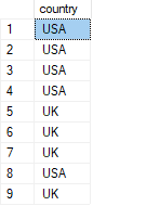
Back to our discussion about duplicates. Despite the fact that the underlying Employees table has a key and hence no duplicates, this table expression which is based on Employees, does have duplicates in its table result:

Run the following code:

USE TSQLV6;

SELECT country FROM HR.Employees;

You get the following output:

Of course, T-SQL does give you tools to eliminate duplicates in a table expression if you want to, it’s just that in some cases it doesn’t do so by default. In the above example, as you know well, you can use the DISTINCT set quantifier for this purpose. People often learn a dialect of SQL like T-SQL without learning the theory behind it. Many are so used to the fact that returning duplicates is the default behavior, that they don’t realize that that’s not really normal in the underlying theory.

Controlling duplicates in T-SQL/SQL

If I tried covering all aspects of controlling duplicates in T-SQL, I’d probably easily end up with dozens of pages. To make this article more approachable, I’ll focus on features that involve using quantifiers to allow or restrict duplicates.

SELECT List

T-SQL allows you to apply a set quantifier ALL | DISTINCT to the SELECT list of a query. The default is ALL if you don’t specify a quantifier.

The earlier query returning the countries where you have employees, without removal of duplicates, is equivalent to the following:

SELECT ALL country FROM HR.Employees;

As you know, you need to explicitly use the DISTINCT quantifier to remove duplicates, like so:

SELECT DISTINCT country FROM HR.Employees;

This code returns the following output:

Aggregate Functions

Similar to the SELECT list’s quantifier, you can apply a set quantifier ALL | DISTINCT to the input of an aggregate function. Also here the ALL quantifier is the default if you don’t specify one explicitly. With the ALL quantifier—whether explicit or implied—redundant duplicates are retained. The following two queries are logically equivalent:

SELECT COUNT(country) AS cnt FROM HR.Employees;

SELECT COUNT(ALL country) AS cnt FROM HR.Employees;

Both queries return a count of 9 since there are nine rows where country is not NULL.

Again, you can use the DISTINCT quantifier if you want to remove redundant duplicates, like so:

SELECT COUNT(DISTINCT country) AS cnt FROM HR.Employees;

This query returns 2 since there are two distinct countries where you have employees.

Note that at the time of writing, T-SQL supports the DISTINCT quantifier with grouped aggregate functions, but not with windowed aggregate functions. There are workarounds, but they are far from being trivial.

Set operators

Set operators allow you to combine data from two input table expressions. The SQL standard supports three set operators UNION, INTERSECT and EXCEPT, each with two possible quantifiers ALL | DISTINCT. With set operators the DISTINCT quantifier is the default if you don’t specify one explicitly.

At the time of writing, T-SQL supports only a subset of the standard set operators. It supports UNION (implied DISTINCT), UNION ALL, INTERSECT (implied DISTINCT) and EXCEPT (implied DISTINCT). It doesn’t allow you to be explicit with the DISTINCT quantifier, although that’s the behavior that you get by default, and it supports the ALL option only with the UNION ALL operator. It currently does not support the INTERSECT ALL and EXPECT ALL operators. I’ll explain all standard variants, and for the missing ones in T-SQL, I’ll provide workarounds.

You apply a set operator to two input table expressions, which I’ll refer to as TE1 and TE2:

TE1
<set operator> 
TE2

The above represents a table expression.

A statement based on a table expression with a set operator can have an optional ORDER BY clause applied to the result, using the following syntax:

TE1 <set operator>  TE2 
[ORDER BY <order by list>];

You’re probably familiar with the set operators that T-SQL supports. Still, let me briefly explain what each operator does:

• UNION: Returns distinct rows that appear in TE1, TE2 or both. That is, if row R appears in TE1, TE2 or both, irrespective of number of occurrences, it appears exactly once in the result.
• UNION ALL: Returns all rows that appear in TE1, TE2 or both. That is, if row R appears m times in TE1 and n times in TE2, it appears m + n times in the result.
• INTERSECT: Returns distinct rows that are common to both TE1 and TE2. That is, if row R appears at least once in TE1, and at least once in TE2, it appears exactly once in the result.
• INTERSECT ALL: Returns all rows that are common to both TE1 and TE2. That is, if row R appears m times in TE1 and n times in TE2, it appears minimum(m, n) times in the result. For example, if R appears 5 times in TE1 and 3 times in TE2, it appears 3 times in the result.
• EXCEPT: Returns distinct rows that appear in TE1 but not in TE2. That is, if a row R appears in TE1, irrespective of the number of occurrences, and does not appear in TE2, it appears exactly once in the output.
• EXCEPT ALL: Returns all rows that appear in TE1 but don’t have an occurrence match in TE2. That is, if a row R appears m times in TE1, and n times in TE2, it appears maximum((m - n), 0) times in the result. For example, if R appears 5 times in TE1 and 3 times in TE2, it appears 2 times in the result. If R appears 3 times in TE1 and 5 times in TE2, it doesn’t appear in the result.

An interesting question is why would you use a set operator to handle a given task as opposed to alternative tools to combine data from multiple tables, such as joins and subqueries? To me, one of the main benefits is the fact that when set operators compare rows, they implicitly use distinctness-based comparison and not equality-based comparison. Recall that distinctness-based comparison handles NULLs and non-NULL values the same way, essentially using two-valued logic instead of three-valued logic. That’s often the desired behavior, and with set operators it simplifies the code a great deal. For example, the following code identifies distinct locations that are both customer locations and employee locations:

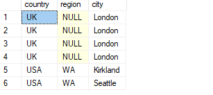
SELECT country, region, city FROM Sales.Customers
INTERSECT
SELECT country, region, city FROM HR.Employees;

This code generates the following output:

Since set operators implicitly use the distinct predicate to compare rows (not to confuse with the fact that without an explicit quantifier they use the DISTINCT quantifier by default), you didn’t need to do anything special to get a match when comparing two NULLs and a nonmatch when comparing a NULL with a non-NULL value. The location UK, NULL, London is part of the result since it appears in both inputs.

Also, with no explicit quantifier specified, a set operator uses an implicit DISTINCT quantifier by default. Remember that with INTERSECT, as long as at least one occurrence of a row appears in both sides, INTERSECT returns one occurrence of the row in the result.

As an exercise, I urge you to write a logically equivalent solution to the above code, using either joins or subqueries. Of course it’s doable, but not this concisely.

As mentioned, the standard also supports an ALL version of INTERSECT. For example, the following standard query returns all occurrences of locations that are both customer locations and employee locations (don’t run it against SQL Server since it’s not supported in T-SQL):

SELECT country, region, city FROM Sales.Customers
INTERSECT ALL
SELECT country, region, city FROM HR.Employees;

If you want to use a solution that is supported in T-SQL, the trick is to compute row numbers in each input table expression to number the duplicates, and then apply the operation to the inputs including the row numbers. You can then exclude the row numbers from the result by using a named table expression like a CTE. Here’s the complete code:

WITH C AS
(
  SELECT country, region, city, 
    ROW_NUMBER() OVER(PARTITION BY country, region, city 
                              ORDER BY (SELECT NULL)) AS rownum
  FROM Sales.Customers
  
  INTERSECT
  
  SELECT country, region, city, 
    ROW_NUMBER() OVER(PARTITION BY country, region, city 
                              ORDER BY (SELECT NULL)) AS rownum
  FROM HR.Employees
)
SELECT country, region, city
FROM C;

This code generates the following output:

The location UK, NULL, London appears 6 times in the first input table expression and 4 times in the second, therefore 4 occurrences intersect.

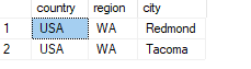
You can handle an except need very similarly. If you’re interested in an except distinct operation, you use the EXCEPT (implied DISTINCT) in T-SQL. For example, the following code returns distinct employee locations that are not customer locations:

SELECT country, region, city FROM HR.Employees
EXCEPT
SELECT country, region, city FROM Sales.Customers;

This code generates the following output:

If you wanted all employee locations that per occurrence don’t have a matching customer location, the standard code for this looks like so:

SELECT country, region, city FROM HR.Employees
EXCEPT ALL
SELECT country, region, city FROM Sales.Customers;

However, T-SQL doesn’t support the ALL quantifier with the EXCEPT operator. You can use a similar trick to the one you used to achieve the equivalent of INTERSECT ALL. You can achieve the equivalent of EXCEPT ALL by applying EXCEPT (implied DISTINCT) to inputs that include row numbers that number duplicate, like so:

WITH C AS
(
  SELECT country, region, city, 
    ROW_NUMBER() OVER(PARTITION BY country, region, city 
                            ORDER BY (SELECT NULL)) AS rownum
  FROM HR.Employees
  
  EXCEPT
  
  SELECT country, region, city, 
    ROW_NUMBER() OVER(PARTITION BY country, region, city 
                            ORDER BY (SELECT NULL)) AS rownum
  FROM Sales.Customers
)
SELECT country, region, city
FROM C;

This code generates the following output:

Curiously, Seattle appears once in this result of except all but didn’t appear at all in the result of the except distinct version. You might initially think that there’s a bug in the code. But think carefully what could explain this? There are two employees from Seattle and one customer from Seattle. The except distinct operation isn’t supposed to return any occurrences in the result, yet the except all operation is indeed supposed to return one occurrence.

Conclusion

Without proper understanding of the foundations of T-SQL—primarily relational theory and its own roots—it’s hard to truly understand what you’re dealing with. In this article I focused on duplicates. A concept that to most seems trivial and intuitive. However, as it turns out, a true understanding of duplicates in T-SQL is far from being trivial.

You need to understand the differences between how relational theory treats duplicates versus SQL/T-SQL. A relation’s body doesn’t have duplicates whereas a table’s body can have those.

It’s very important to understand the difference between distinctness-based comparison, such as when using the distinct predicate explicitly or implicitly, versus equality-based comparison. Then you realize that in T-SQL, two comparands are duplicates when one is not distinct from the other.

You also need to understand the nuances of how T-SQL handles duplicates, the cases where it retains redundant ones versus cases where it removes those. You also need to understand the tools that you have to change the default behavior using quantifiers such as DISTINCT and ALL.

I discussed controlling duplicates in a query’s SELECT list, aggregate functions and set operators. But there are other language elements where you might need to control them such as handling ties with the TOP filter, window functions, and others.

What I hope that you take away from this article is the significance of investing time and energy in learning the fundamentals. And if you haven’t had enough of T-SQL Fundamentals, and I’m allowed a shameless plug, check out my new book T-SQL Fundamentals 4th Edition.

May the 4th be with you!

 

The post T-SQL Fundamentals: Controlling Duplicates appeared first on Simple Talk.

from Simple Talk https://ift.tt/zn5NIH8
via

Microsoft Fabric and the Delta Tables Secrets

Microsoft Fabric storage uses OneLake and Delta Tables, the core storage of all Fabric objects, as explained in my introduction to Microsoft Fabric.

Either if you use lakehouses, data warehouses, or even datasets, all the data is stored in the OneLake. OneLake uses Delta Tables as storage. In this way, we need to be aware of some “secrets” related to delta table storage in order to make the best decisions possible for our data platform solution.

Let’s analyze some of the Parquet and Delta Table behaviors.

Parquet and Delta

Parquet is an open source format which became famous as one of the most used formats in data lakes. It’s a columnar storage format intended to store historical data.

One very important “secret”, and the main subject of this blog is: Parquet format is immutable. It’s not possible to change the content of a Parquet file. It’s intended for historical data.

Although the main objective is for historical data, many people and companies worked on this problem. The result was Delta Tables.

Delta Tables use the Parquet format, it’s not a different format. The immutable behavior continues. However, Delta Tables use an additional folder as a transaction log. The operations are registered in the delta logs, marking records with updates and deletes.

In this way, the underlying immutable behavior is still present, but we can work with the data in a transactional way, allowing updates and deletes, for example.

Time Travel

The delta logs allow us to make what’s called Time Travel. We can retrieve the information from a delta table in the way it was on a specific date and time, as long as the logs are kept complete.

The access to the entire historical of data changes is an important resource for a data storage.

Data Modelling

The need to keep historical data is way older than technologies such as Delta Time Travel, which allow us to keep them. The Data Modelling techniques, such as Data Warehouse modelling, proposed solutions for historical storage a long time ago.

One of the features used for this purpose is called Slowly Changing Dimensions, or Dimension Type 2. When we design a start schema, we decide which dimensions should keep an entire history and which ones aren’t worth the trouble and a simple update on the records would be enough.

For example, let’s consider a dimension called Customer. If we decide to keep the dimension as a SCD dimension, every time a customer record is changed in production, we create a new version of the record in the intelligence storage (data warehouse, data lake, whatever the name).

On the other hand, if we decide that a dimension is not worth keeping a history, we can just update the record in the intelligence storage when needed.

The decision of using a SCD dimension or not, and many more, are all made during modelling. They are independent of any technical feature capable of keeping the history of the data. The history is designed during modelling and kept by us.

Choosing Between Time Travel and Data Modelling

We have the possibility to use data modelling to control the history of our storage, or use the technical features, such as Time Travel.

This leads to several possibilities with different consequences:

Approach	Possible Results
We can choose to rely on time travel for the entire history storage of our data	This will tie the history of your data solution with a specific technological feature. It also creates the risk of performance issues related to executing updates in a delta table. Let’s talk more in depth about the technology and leave the decision to you.
We can choose to rely on the modelling for the entire history and not depend on the time travel feature	This creates additional modelling and ingestion work, plus additional work to avoid performance issues with the delta log. The work to avoid performance issues with the delta log may be easier than if we were really relying on it.

The decision whether we should rely on modelling, on technology or stay somewhere in the middle is complex enough to generate many books. What’s important on this blog is to understand the decision is present when designing an architecture with Microsoft Fabric.

In order to make a well-informed decision, we need to understand how the delta tables process updates/deletes.

Lakehouse Example

The example will be made using a table called Fact_Sale. You can use a pipeline to import the data from https://ift.tt/bJBmN0R to the files area of one Fabric Lakehouse. The article about Lakehouse and ETL explains how to build a pipeline to bring data to the Files area.

The article https://www.red-gate.com/simple-talk/blogs/microsoft-fabric-using-notebooks-and-table-partitioning-to-convert-files-to-tables/ explains this import process and how we can partition the data by Year and Quarter, making a more interesting example. The notebook code to import the partitioned data to the Tables area of the lakehouse is the following:

from pyspark.sql.functions import col, year, month, quarter
table_name = 'fact_sale'
df = spark.read.format("parquet").load('Files/fact_sale_1y_full')
df = df.withColumn('Year', year(col("InvoiceDateKey")))
df = df.withColumn('Quarter', quarter(col("InvoiceDateKey")))
df = df.withColumn('Month', month(col("InvoiceDateKey")))
df.write.mode("overwrite").format("delta").partitionBy("Year","Quarter").save("Tables/" + table_name)

The default size for a Parquet file in the Fabric environment is 1GB (1073741824 bytes). This is defined by the session configuration spark.microsoft.delta.optimizeWrite.binSize and has the purpose to avoid the delta lake small files problem. Although this is a common problem, the writing on delta tables can cause consequences when the file is too big. Let’s analyze this as well.

You can find more about Spark configuration on this blog and more about the small files problem on this link.

On our example, this configuration generated a single parquet file for each quarter, this will help to identify what’s happening during the example.

The Data we Have

We need to identify the total of records we have, the total records for each quarter, and the minimum and maximum SalesKey value in each quarter in order to build the example.

We can use the SQL Endpoint to run the following queries:

SELECT Count(*) AS TotalRecords
FROM   fact_sale 

SELECT quarter,
       Count(*)     SalesCount,
       Min(salekey) MinKey,
       Max(salekey) MaxKey
FROM   fact_sale
GROUP  BY quarter 

Test query and Execution Time

For test purposes, let’s use the following query:

SELECT customerkey,
       Sum(totalincludingtax) TotalIncludingTax
FROM   fact_sale
GROUP  BY customerkey 

This query makes a grouping on all our records by CustomerKey, across the quarter partitions, creating a total of Sales by customer. On each test, I will execute this query 10 times and check the initial, minimum, and maximum execution time.

 

First 10 Executions
Initial	2.639 seconds
Minimum	1.746 seconds
Maximum	3.32 seconds
Average	2.292 seconds

Updating one single record

As the first test, let’s update one single sales record in each quarter. We will use a notebook to execute the following code:

%%sql
update fact_sale set TotalIncludingTax=TotalIncludingTax * 2
where SaleKey = 6000000;

update fact_sale set TotalIncludingTax=TotalIncludingTax * 2
where SaleKey = 15624569 ;

update fact_sale set TotalIncludingTax=TotalIncludingTax * 2
where SaleKey = 35270205;

update fact_sale set TotalIncludingTax=TotalIncludingTax * 2
where SaleKey = 45032105;

After executing these updates, if you look on the table Parquet files, you will notice each parquet file containing the record updated was duplicated.

The parquet file continues to be immutable, in order to update a record, the entire file is duplicated with the record update and the delta logs register this update.

In our example, we updated 4 records, but each one was in a different parquet file. As a result, all the parquet files were duplicated (one for each quarter).

Remember the default file size is 1GB. A single record update will result in the duplication of a 1GB file. The big file size may have a bad side effect if you decide to use upserts or deletes too much.

Testing the Execution

Let’s test the execution of our sample query again and get the number after these duplication of parquet files:

After Updating 1 record
Initial	6.692 seconds
Minimum	1.564 seconds
Maximum	3.166 seconds (ignoring initial)
Average	2.8955 seconds
Average Ignoring Initial	2.4374 seconds

There is a initial execution substantially slower and the average, even ignoring the initial execution, is slower, but not much.

Updating many records

Let’s change a bit the script and update a higher volume of records each quarter. You can execute the script below many times and each time you execute you will see the parquet files being duplicated.

%%sql
update fact_sale set TotalIncludingTax=TotalIncludingTax * 2
where SaleKey < 7000000;

update fact_sale set TotalIncludingTax=TotalIncludingTax * 2
where SaleKey > 14624564 AND SaleKey < 18624564;

update fact_sale set TotalIncludingTax=TotalIncludingTax * 2
where SaleKey > 28270201 AND SaleKey < 35270201;

update fact_sale set TotalIncludingTax=TotalIncludingTax * 2
where SaleKey > 42032102 AND SaleKey < 45032102;

Result

After executing the update script 4 times, we end up with 6 files on each partition. The original file, the file created by the update of a single record and the 4 files created when updating multiple record.

These are the results of the test query execution:

After Updating 1 record
Initial	11.894 seconds
Minimum	1.553 seconds
Maximum	2.286 seconds (ignoring initial)
Average	2.9394 seconds
Average Ignoring Initial	1.9494 seconds

The test seems to illustrate only the initial query is affected and affected a lot. After the data is in cache, the files in the delta table don’t affect the query, or at least, it seems so.

On one hand, this illustrates the problem. On the other hand, we are talking about a few seconds difference for a set of 50 million records.

Cleaning the Table

The process of cleaning the table from unlinked parquet files is executed by the statement VACUUM. There are some important points to highlight about this process:

• If you decide to manage yourself the data history using data modelling, this needs to be a regular process on tables affected by updates and deletes.
• On the other hand, if you decide to use Time Travel to manage history, you can’t execute this process, otherwise you will lose the time travel capability.

This process needs to be executed very carefully. You can’t try to delete files while you have some process in execution over the data. You need to ensure this will only be executed while you don’t have anything running over the data.

The default method to ensure this is to only delete files older than one specific time. For example, if you want to delete unlinked files younger than 168 hours, you need to activate a special spark session configuration to ensure you are aware about what you are doing.

In this way, the example below, which activates this configuration and executes the VACUUM with 0 retention, is only for test purposes, not for production scenarios.

spark.conf.set("spark.databricks.delta.retentionDurationCheck.enabled", "false")

 

 

%%sql
VACUUM 'Tables/fact_sale' RETAIN 0 HOURS

After executing this cleaning, the additional files will disappear and only the most updated will remain.

Onelake is for all

This process affects not only the lakehouse, but the data warehouse as well. In the lakehouse, the SQL Endpoint is read-only, but the Data Warehouse is read-write with MERGE operations.

Conclusion

Microsoft Fabric is a PaaS environment for the entire Enterprise Data Architecture and capable of enabling the most modern architectures, such as Data Mesh.

However, we should never lose track of the data concepts, such as the fact the data intelligence storage is intended to be read-only and for historical purposes. Our architectural decisions may have an impact on the result which may not be so obvious in a PaaS environment.

The post Microsoft Fabric and the Delta Tables Secrets appeared first on Simple Talk.

from Simple Talk https://ift.tt/a9T8A5N
via

MySQL joins

Tables in a MySQL database are commonly related to one another, often in multiple ways, and it is only by linking the tables together that you can derive meaningful information from the data. To connect these tables together, you can use the JOIN clause, which you include in your SELECT, DELETE, or UPDATE statements. The clause provides a structure for connecting the data from multiple tables, letting you specify which tables to join and under what conditions to join them.

MySQL supports three basic types of joins: inner joins, outer joins, and cross joins. Outer joins can be further broken down to left outer joins and right outer joins. You can also use left and right joins together to create full outer joins. In this article, I explain how to add joins to your SELECT statements and provide examples that demonstrate how they work. Each example retrieves data from the manufacturers and airplanes tables in the travel database, which you’ve seen in previous articles in this series.

Note: The examples in this article are based on a local instance of MySQL that hosts a very simple database. The last section of the article—“Appendix: Preparing your MySQL environment”—provides information about how I set up my environment and includes a SQL script for creating the database I used when building these examples.

MySQL inner joins

An inner join can retrieve matching data from multiple tables based on one or more columns that are common to both tables. For example, the manufacturers and airplanes tables in the travel database each contain the manufacturer_id column. You can create an inner join that links the data in the two tables together based on the values in those columns. The join will return all rows with matching manufacturer_id values. The following figure shows how you might visualize an inner join between the two tables.

The left circle represents the data in the manufacturers table, and the right circle represents the data in the airplanes table. The area in which they intersect is where the manufacturer_id values in the manufacturers table are equal to the manufacturer_id values in the airplanes table.

Note: if you are well acquainted with Venn diagrams, you know they generally work with complete sets of data. They help visualize which rows will be returned in the join operation but note that only the column values in the join condition are part of the intersection (for an INNER JOIN operation) and the other combinations that will be included.

An inner join returns only the matching rows from the two tables and excludes all other rows. You’ll see this in action shortly, but first take a look at the following syntax, which represents a SELECT statement and its INNER JOIN clause at their most basic:

SELECT select_list
FROM tbl_1 [[AS] tbl_1_alias]
  [INNER] JOIN tbl_2 [[AS] tbl_2_alias]
  [ON tbl_1_col = tbl_2_col];

The first two lines in the syntax are similar to most other SELECT statements. They define the SELECT clause and the initial part of the FROM clause. The third line represents the start of JOIN clause, which is actually a subclause in the FROM clause. The JOIN clause specifies the name of the second table. This is the table that will be joined to the first table.

The fourth line in the syntax shows the ON clause. Although the clause is technically optional, it is typically included when defining an inner join because it will behave as if the join criteria is always the Boolean value of True. Later in the article, I’ll discuss joins that don’t include the ON clause on purpose, but for now, assume that you’ll be including it all of your queries that you expect to be an INNER JOIN. The clause defines a search condition that determines how the tables are joined.

The syntax shows how the ON clause is commonly structured. It defines a value equality expression which states that a column in the first table must equal a column in the second table. You can create other types of expressions, but for this article, we’ll focus only on value equality expressions because those are the most common.

The following example demonstrates how the various syntax elements plug into an actual SELECT statement:

SELECT m.manufacturer, a.plane, a.engine_type, a.icao_code
FROM manufacturers AS m INNER JOIN airplanes AS a
  ON m.manufacturer_id = a. manufacturer_id;

After the SELECT clause, the statement defines a FROM clause, which starts by specifying the manufacturers table and assigning it the m alias. A table alias can be useful when referencing the table’s individual columns in other clauses, such as the SELECT clause (and essential if you need to reference the same table twice). Otherwise, you would need to include the entire table name to ensure that there is no ambiguity between columns from different table. Theoretically, you do not need to qualify a name if it is unique among the joined tables, but many database and development teams consider its inclusion a best practice.

The FROM clause then goes on to define the INNER JOIN clause. It identifies airplanes as the second table and assigns it the alias a. Next comes the ON clause and its search condition, which specifies that the m.manufacturer_id values must equal the a.manufacturer_id values for the rows to be returned. In other words, the clause limits the statement’s results to only those rows with matching manufacturer_id values. The following figure shows the data returned by the SELECT statement.

Because the query returns only those rows with matching manufacturer_id values, the results do not include manufacturers in the manufacturers table for which there are no matching planes in the airplanes table, nor do they include planes in the airplanes table for which there are no matching manufacturers in the manufacturers table.

Now let’s move on to the AS keyword, which the example above uses when defining the table aliases. You do not need to include this keyword. For example, you can recast the previous SELECT statement as follows:

SELECT m.manufacturer, a.plane, a.engine_type, a.icao_code
FROM manufacturers m INNER JOIN airplanes a
  ON m.manufacturer_id = a. manufacturer_id;

You also do not need to include the INNER keyword in your JOIN clause. When JOIN is used without INNER, MySQL assumes that you want to perform an inner join. The following example returns the same results as the previous two SELECT statements:

SELECT m.manufacturer, a.plane, a.engine_type, a.icao_code
FROM manufacturers m JOIN airplanes a
  ON m.manufacturer_id = a. manufacturer_id;

The fact that you do not need to include the INNER keyword indicates that MySQL considers an inner join to be the most natural type of join. In fact, MySQL supports something called a “natural join,” which you can use in place of an inner join when the compared columns have the same name and datatype, as in the following example:

SELECT m.manufacturer, a.plane, a.engine_type, a.icao_code
FROM manufacturers m NATURAL JOIN airplanes a;

The SELECT statement returns the same results as the previous statements even though it does not include an ON clause. Be aware, however, that a natural join, unlike an inner join, removes duplicate columns, such as those you get with a SELECT * query. In this case, the natural join returns only one manufacturer_id column, rather than one from each table. In contrast, the inner join returns both columns. Also note that if your tables share other column names (name, row_last_modified_time, for example,) a NATURAL JOIN will not work properly.

Note: MySQL joins are a complex topic. This article focuses only on creating joins that combine two tables, basing the joins on a single set of matching columns. While you can only join two tables at a time, you can join more than two tables in a statement, and you can base your joins on more than one set of matching columns. You can also define other types of search criteria in your ON clauses (other than value equality). For more information about joins, see the MySQL documentation, starting with the JOIN Clause topic.

The examples that we’ve looked at up to this point have included only a SELECT clause and a FROM clause, which contained the join definition. You can include other clauses, however, just like you can in any SELECT statement. For example, the following SELECT statement includes a WHERE clause and ORDER BY clause:

SELECT m.manufacturer, a.plane, a.engine_type, a.max_weight
FROM manufacturers AS m INNER JOIN airplanes AS a
  ON m.manufacturer_id = a. manufacturer_id
WHERE a.max_weight < 10000
ORDER BY a.max_weight DESC;

The statement now returns only six rows, which are shown in the following figure. As expected, all the returned data meets the condition defined in the WHERE clause.

You can also group and aggregate the data returned by your joined tables. The next SELECT statement groups the data based on the manufacturer_id values in the manufacturers table and then aggregates the data in those groups:

SELECT m.manufacturer_id, m.manufacturer, 
  ROUND(AVG(a.max_weight)) AS avg_weight
FROM manufacturers AS m INNER JOIN airplanes AS a
  ON m.manufacturer_id = a. manufacturer_id
GROUP BY m.manufacturer_id
ORDER BY avg_weight DESC;

In this case, the SELECT clause calculates the average max_weight value for the planes associated with each manufacturer and assigns the avg_weight alias to the generated column. The following figure shows the results returned by the SELECT statement.

Be aware of the cardinality of rows in your output when you are aggregating data. For example, this was the raw data when we joined the tables together:

Note: If you count the number of manufacturers using this set of data, you will get 12, while there are just 4. Generally, the table with the key value you are joining on will be the one that you need to use in the GROUP BY clause, and the table referencing that table will be the one that you need to use in aggregate functions like AVG, SUM, MIN, MAX, etc.

MySQL also supports the USING clause when defining a join condition, which you use in place of the ON clause. You can include the USING clause only if the matching columns have the same names and are configured with the same data type. This is useful when the same name is used in both tables, but you have additional columns with the same name as well. The USING clause is safer to use than a NATURAL JOIN in reusable code because it is not susceptible to new, duplicated columns.

The manufacturer_id columns in the manufacturers and airplanes tables meet the requirement, so you can recast the previous SELECT statement as follows:

SELECT m.manufacturer_id, m.manufacturer, 
  ROUND(AVG(max_weight)) AS avg_weight
FROM manufacturers AS m INNER JOIN airplanes AS a
  USING (manufacturer_id)
GROUP BY m.manufacturer_id
ORDER BY avg_weight DESC;

When specifying the column in the USING clause, you must enclose it in parentheses. In addition, you should not qualify the column name with a table name or alias as you do in an ON clause. You simply specify the column name.

MySQL left and right outer joins

In some cases, you might want to retrieve the non-matching data from one of the joined tables, along with the matching data from both tables. To do so, you should define an outer join rather than an inner join.

MySQL supports two types of outer joins: left outer joins and right outer joins. The “left” refers to the left table specified in the JOIN clause, and the “right” refers to the right table specified in the clause. In a left outer join, non-matching rows in the left table are included in the results, and in a right outer join, non-matching rows in the right table are included in the results.

For example, the following figure shows you how you might visualize a left outer join between the manufacturers and airplanes tables.

As you saw with inner joins, the left circle represents the manufacturers table, which is the “left” table, and the right circle represents the airplanes table, which is the “right” table. The area in which they intersect is where the manufacturer_id values in both tables match. The join also incorporates the non-matching data in the left table, which is indicated by the solid green.

Creating an outer join works much like an inner join. The following syntax shows a basic SELECT statement that includes the LEFT OUTER JOIN clause:

SELECT select_list
FROM tbl_1 [[AS] tbl_1_alias]
  LEFT [OUTER] JOIN tbl_2 [[AS] tbl_2_alias]
  [ON tbl_1_col = tbl_2_col];

The syntax is similar to an inner join except for the use of the LEFT keyword and optional OUTER keyword. The syntax is meant to show only the most basic elements necessary to perform a left outer join. It does not reflect other clauses that you can add to your SELECT statements, such as WHERE or GROUP BY. For example, the following query creates a left outer join with the manufacturers table specified as the left table:

SELECT m.manufacturer_id, m.manufacturer, a.plane, 
  a.engine_type, a.max_weight, a.wingspan
FROM manufacturers AS m 
  LEFT OUTER JOIN airplanes AS a
  ON m.manufacturer_id = a. manufacturer_id
ORDER BY a.plane;

In addition to the JOIN clause, the also includes an ORDER BY clause that sorts the data by the plane column, in ascending order. The SELECT statement returns the result set shown in the following figure.

In addition to the matching rows, the statement returns all rows from the manufacturers table for which there is no matching data in the airplanes table. You can identify these rows by the NULL values in the columns from the airplanes table. In this case, the first three rows have no matching data. However, the rest of the rows in the left table match rows in the right table, so those results look much like you saw with the inner joins.

MySQL also lets you include a USING clause in your outer join statements, just like you can your inner joins. For example, you can recast the previous SELECT statement to include a USING clause, which returns the same results:

SELECT m.manufacturer_id, m.manufacturer, a.plane, 
  a.engine_type, a.max_weight, a.wingspan
FROM manufacturers AS m 
  LEFT OUTER JOIN airplanes AS a
  USING (manufacturer_id)
ORDER BY a.plane;

A right outer join works just like a left outer join except that it returns non-matching rows from the right table rather than the left table, as illustrated in the following figure. Once again, the area in which the two circles intersect is where the manufacturer_id values in the two tables match. The solid part of the right circle represents the non-matching data in the right table.

A right outer join is simply the reverse of a left outer join. They can be used interchangeably by reversing the table order. In fact, MySQL documentation recommends that you stick with left joins for all your outer joins: “RIGHT JOIN works analogously to LEFT JOIN. To keep code portable across databases, it is recommended that you use LEFT JOIN instead of RIGHT JOIN.” If you take this approach, you need only reverse the order of the tables when building your queries.

While generally a good approach, despite the MySQL recommendations there might be times when you need to use a right outer join, such as when you are joining multiple tables, or when you’re constructing a full outer join (which I’ll demonstrate shortly). The following syntax shows a basic SELECT statement that includes the RIGHT OUTER JOIN clause:

SELECT select_list
FROM tbl_1 [[AS] tbl_1_alias]
  RIGHT [OUTER] JOIN tbl_2 [[AS] tbl_2_alias]
  [ON tbl_1_col = tbl_2_col];

The syntax differs from the left outer join only in the use of the RIGHT keyword rather than the LEFT keyword. The SELECT statement in the following example demonstrates what this looks like:

SELECT m.manufacturer_id AS man_tbl_id, m.manufacturer, 
  a.plane_id, a.plane, a.manufacturer_id AS air_tbl_id
FROM manufacturers AS m 
  RIGHT OUTER JOIN airplanes AS a
  ON m.manufacturer_id = a. manufacturer_id
ORDER BY a.plane;

In this example, I included the manufacturer_id column from both tables, providing a different alias for each one. This makes it easier to distinguish between the two columns and to see which manufacturer_id values exist in the airplanes table that do not exist in the manufacturers table. The following figure shows the results returned by the SELECT statement.

As the figure demonstrates, the airplanes table contains six non-matching rows, which are indicated by the NULL values in the man_tbl_id and manufacturer columns, both of which come from the manufacturers table.

Note that the examples for this article are not necessarily best practices in database design. However, to demonstrate some of the different join types, it was necessary to have rows in each table that did not relate to one another.

In some cases, you might need to perform an outer join that returns only the non-matching rows in one of the tables. For example, you might want to know which rows in the airplanes table reference manufacturer_id values that do not exist in the manufacturers table, as illustrated in the following figure.

You can retrieve this information by adding a WHERE clause to your SELECT statement that checks the data for nullability. In effect, you’re taking advantage of the NULL values returned by your query when there are no corresponding matches. For example, the following SELECT statement is the same as the previous one except that it includes a WHERE clause:

SELECT a.plane_id, a.plane, a.manufacturer_id
FROM manufacturers AS m 
  RIGHT OUTER JOIN airplanes AS a
  ON m.manufacturer_id = a. manufacturer_id
WHERE m.manufacturer IS NULL
ORDER BY a.plane;

The WHERE clause uses the IS NULL operator to check whether the manufacturer_id column contains a NULL value. If it does, the expression evaluates to true and the row is returned, giving us the results shown in the following figure.

Checking for NULL values in this way provides a handy method for identifying what might be anomalous data, which could be the result of a bulk-loading operation, merging tables from a legacy system, a bug at the application or data level, or some other process.

Where filtering by NULL finds the values that don’t match, be careful about filtering rows in the WHERE clause unless you realize what you are doing. For example, executing the following:

SELECT m.manufacturer_id, m.manufacturer, a.plane, 
  a.engine_type, a.max_weight, a.wingspan
FROM manufacturers AS m 
  LEFT OUTER JOIN airplanes AS a
  USING (manufacturer_id)
WHERE a.manufacturer_id = 104 -- where clause filter
ORDER BY a.plane;

Will just return the rows with manufacturer = 104. This, in effect, turns this into an INNER JOIN, because all of the mismatched rows from the LEFT OUTER JOIN will be eliminated because their manufacturer_id is NULL and hence, does not equal 104. However, change your join to:

SELECT m.manufacturer_id, m.manufacturer, a.plane, 
  a.engine_type, a.max_weight, a.wingspan
FROM manufacturers AS m 
  LEFT OUTER JOIN airplanes AS a
  ON m.manufacturer_id = a.manufacturer_id
     AND a.manufacturer_id = 104
ORDER BY a.plane;

And the output is changed again, but perhaps not exactly what you wanted as now every manufacturer is returned, but only rows that match the a.manufacturer_id = 104 predicate are returned.

MySQL full outer joins

A full outer join returns all data from the two connected tables. In addition to the matching rows from both tables, the join returns unmatched rows in the left table and unmatched rows in the right table, as illustrated in the following figure. In this case, the result set includes manufacturers with no corresponding planes in the airplanes table and planes with no corresponding manufacturers in the manufacturing table, along with the matching data from both tables.

MySQL does not support full outer joins like some database systems. You can get around this by using a UNION operator to join a left outer join statement and a right outer join statement, as in the following example:

SELECT m.manufacturer, a.plane, a.engine_type
FROM manufacturers AS m 
  LEFT OUTER JOIN airplanes AS a
  USING (manufacturer_id)
UNION ALL
SELECT m.manufacturer, a.plane, a.engine_type
FROM manufacturers AS m 
  RIGHT OUTER JOIN airplanes AS a
  USING (manufacturer_id);

The individual SELECT statements work just like the earlier examples of left and right outer joins. The UNION ALL operator joins the two statements together to return a single result set, which is shown in the following figure.

The results include both matching rows and non-matching rows, which are indicated by the NULL values. However, because the two statements are joined together, the results also include duplicate rows. For example, the Airbus planes are each listed twice, as are all the other planes. You can eliminate the duplicates by using the UNION operator without the ALL qualifier, as in the following example:

SELECT m.manufacturer, a.plane, a.engine_type
FROM manufacturers AS m 
  LEFT OUTER JOIN airplanes AS a
  USING (manufacturer_id)
UNION
SELECT m.manufacturer, a.plane, a.engine_type
FROM manufacturers AS m 
  RIGHT OUTER JOIN airplanes AS a
  USING (manufacturer_id);

Now the statement returns only distinct rows, whether the data is matching or non-matching, as shown in the following figure:

Although MySQL doesn’t provide a specific clause for creating full outer joins, such as you’ll find in SQL Server or other database systems, there might be times when you need a more complete picture than what either a left outer join or right outer join can provide on its own. Using a UNION operator to combine the two outer joins is a handy way to accomplish this.

MySQL cross joins

Another type of join that MySQL supports is the cross join, which matches each row in the left table to each row in the right table to produce what is referred as a Cartesian product. The following figure illustrates a cross join between the manufacturers table and the airplanes table.

The figure shows the various ways that each value pair can be matched. For example, the 101 value in the manufacturers table is matched to every value in the airplanes table, and the 1001 value in the airplanes table is matched to every value in the manufacturers table. This process continues for each value in both tables until all values have been matched up. The following syntax shows a basic SELECT statement that includes the CROSS JOIN clause:

SELECT select_list
FROM tbl_1 [[AS] tbl_1_alias]
  CROSS JOIN tbl_2 [[AS] tbl_2_alias]
  [ON tbl_1_col = tbl_2_col];

Except for the CROSS keyword, the syntax elements should all look familiar to you. That said, the cross join is not as clear-cut as it might appear. Notice that the syntax, like the previous join examples, indicates that the ON clause is optional. A cross join statement returns a Cartesian product only if it does not include this clause. If the clause is included, the statement behaves much like a regular inner join.

Some sources imply that a MySQL cross join is strictly limited to producing a Cartesian product, but this is clearly not the case, as indicated by its support for the ON clause (or USING clause). According to MySQL documentation, “JOIN, CROSS JOIN, and INNER JOIN are syntactic equivalents (they can replace each other). In standard SQL, they are not equivalent. INNER JOIN is used with an ON clause, CROSS JOIN is used otherwise.”

Let’s look at a few examples to better understand how the cross join works. The following SELECT statement defines a cross join without including an ON clause or USING clause:

SELECT m.manufacturer_id, m.manufacturer, 
  a.plane_id, a.plane, a.manufacturer_id
FROM manufacturers AS m 
  CROSS JOIN airplanes AS a
ORDER BY m.manufacturer_id, a.plane_id;

The statement returns a Cartesian product for the manufacturers and airplanes tables. The manufacturers table contains seven rows, and the airplanes table contains 18 rows. Because a cross join matches each row in the first table to each row in the second table, you can multiply the two row counts together (7 x 18) to calculate the total number of rows that should be included in the Cartesian product. In this case, the total is 126, which is the number of rows returned by the SELECT statement.

The following figure shows a small portion of these results. Notice that there is an Airbus row for each plane, even if that plane is not manufactured by Airbus. The same is true for all manufacturers. The cross join simply combines the individual rows together.

This in itself should seem straightforward enough, and by all accounts, this is how you should use the cross join—to return a Cartesian product. However, because CROSS JOIN and INNER JOIN are syntactic equivalents, you can achieve the same results with an inner join that does not include an ON clause or USING clause:

SELECT m.manufacturer_id, m.manufacturer, 
  a.plane_id, a.plane, a.manufacturer_id
FROM manufacturers AS m 
  INNER JOIN airplanes AS a
ORDER BY m.manufacturer_id, a.plane_id;

The statement returns the same Cartesian product as the previous example. However, this is not the only way to return these results. You can instead specify the two table names, separated by a comma, and drop the JOIN clause altogether:

SELECT m.manufacturer_id, m.manufacturer, 
  a.plane_id, a.plane, a.manufacturer_id
FROM manufacturers m, airplanes a
ORDER BY m.manufacturer_id, a.plane_id;

Once again, you’ll end up with the same Cartesian product that was returned by the previous two examples.

Note: MySQL documentation warns that the precedence of a comma operator is less than the actual JOIN keywords. This might be an issue if you mix join types in a statement that combines more than two tables.

In addition, the comma operator can be used only to generate a Cartesian product. It cannot be used with an ON or USING clause. This is not the case for a cross join, which can include either of these clauses, just like an inner join. The following examples shows a cross join that contains a USING clause:

SELECT m.manufacturer_id, m.manufacturer, 
  a.plane_id, a.plane, a.manufacturer_id
FROM manufacturers AS m 
  CROSS JOIN airplanes AS a
  USING (manufacturer_id)
ORDER BY m.manufacturer_id;

By adding the USING clause, the statement now returns only 12 rows, rather than 126. The results are shown in the following figure.

You can return the same results with the following inner join statement, which also incorporates the USING clause:

SELECT m.manufacturer_id, m.manufacturer, 
  a.plane_id, a.plane, a.manufacturer_id
FROM manufacturers AS m 
  INNER JOIN airplanes AS a
  USING (manufacturer_id)
ORDER BY m.manufacturer_id;

Despite the fact that CROSS JOIN and INNER JOIN are syntactic equivalents, the general consensus is to use cross joins when you want to work directly with the Cartesian product and use inner joins when you want to qualify the join with an ON or USING clause. This doesn’t preclude the use of other SELECT clauses in your cross join statements (such as WHERE or ORDER BY), but it does serve as general guideline for differentiating between the two when you want to generate a Cartesian product.

Getting started with MySQL joins

The topic of MySQL joins is a complex one, as I noted earlier. A single article is not nearly enough to cover all the various ways you can use joins to combine data from multiple tables. Although the article provides you with a jumping-off point, it by no means covers every aspect of join creation. You can, for example, combine different types of joins into a single query, define joins in your DELETE and UPDATE statements, join three or more tables in a single statement, or base your joins on two or more sets of matching columns. To do all this, however, you need a good foundation on which to build, and this article might help you get started with that process.

Appendix: Preparing your MySQL environment

For the examples for this article, I used a Mac computer that was set up with a local instance of MySQL 8.0.29 (Community Server edition). I also used MySQL Workbench to interface with MySQL. Through Workbench, I created the travel database, added the manufacturers and airplanes tables, and inserted test data into the tables.

If you want to try out the examples for yourself, start by running the following script against your MySQL instance:

DROP DATABASE IF EXISTS travel;
CREATE DATABASE travel;
USE travel;
CREATE TABLE manufacturers (
  manufacturer_id INT UNSIGNED NOT NULL,
  manufacturer VARCHAR(50) NOT NULL,
  create_date TIMESTAMP NOT NULL DEFAULT CURRENT_TIMESTAMP,
  last_update TIMESTAMP NOT NULL 
    DEFAULT CURRENT_TIMESTAMP ON UPDATE CURRENT_TIMESTAMP,
  PRIMARY KEY (manufacturer_id) );
CREATE TABLE airplanes (
  plane_id INT UNSIGNED NOT NULL,
  plane VARCHAR(50) NOT NULL,
  manufacturer_id INT UNSIGNED NOT NULL,
  engine_type VARCHAR(50) NOT NULL,
  engine_count TINYINT NOT NULL,
  max_weight MEDIUMINT UNSIGNED NOT NULL,
  wingspan DECIMAL(5,2) NOT NULL,
  plane_length DECIMAL(5,2) NOT NULL,
  parking_area INT GENERATED ALWAYS AS ((wingspan * plane_length)) STORED,
  icao_code CHAR(4) NOT NULL,
  create_date TIMESTAMP NOT NULL DEFAULT CURRENT_TIMESTAMP,
  last_update TIMESTAMP NOT NULL 
    DEFAULT CURRENT_TIMESTAMP ON UPDATE CURRENT_TIMESTAMP,
  PRIMARY KEY (plane_id));

The script creates the travel database and adds the manufacturers and airplanes tables. In previous articles, I had defined a primary key on the airplanes table that referenced the manufacturers table. For this article, I did not include the foreign key so it would be easier to demonstrate various join operations.

After you create the tables, you should run the following INSERT statements:

INSERT INTO manufacturers (manufacturer_id, manufacturer)
VALUES (101,'Airbus'), (102,'Beagle Aircraft Limited'), (103,'Beechcraft'),
  (104,'Boeing'), (105,'Cessna'), (106,'Embraer'), (107,'Gulfstream');
INSERT INTO airplanes 
  (plane_id, plane, manufacturer_id, engine_type, engine_count, 
    wingspan, plane_length, max_weight, icao_code)
VALUES
  (1001,'A340-600',101,'Jet',4,208.17,247.24,837756,'A346'),
  (1002,'A350-800 XWB',101,'Jet',2,212.42,198.58,546700,'A358'),
  (1003,'A350-900',101,'Jet',2,212.42,219.16,617295,'A359'),
  (1004,'A.109 Airedale',102,'Piston',1,36.33,26.33,2750,'AIRD'),
  (1005,'A.61 Terrier',102,'Piston',1,36,23.25,2400,'AUS6'),
  (1006,'B.121 Pup',102,'Piston',1,31,23.17,1600,'PUP'),
  (1007,'Baron 56 TC Turbo Baron',103,'Piston',2,37.83,28,5990,'BE56'),
  (1008,'Bonanza 33 (F33A)',103,'Piston',1,33.5,26.67,3500,'BE33'),
  (1009,'Bonanza 35 (G35)',103,'Piston',1,32.83,25.17,3125,'BE35'),
  (1010,'747-8F',104,'Jet',4,224.42,250.17,987000,'B748'),
  (1011,'747-SP',104,'Jet',4,195.67,184.75,696000,'B74S'),
  (1012,'757-300',104,'Jet',2,124.83,178.58,270000,'B753'),
  (1013,'PA-28R-200 Cherokee Arrow',121,'Piston',1,30.00,23.50,2600,'P28R'),
  (1014,'PA-18-150 Super Cub',121,'Piston',1,35.29,22.50,1750,'PA18'),
  (1015,'PA-24-180 Comanche',121,'Piston',1,36.00,24.79,2550,'PA24'),
  (1016,'M20D Master',136,'Piston',1,35.00,23.25,2500,'M20P'),
  (1017,'M20F Executive 21',136,'Piston',1,36.00,24.00,2740,'M20P'),
  (1018,'M20L PFM',136,'Piston',1,36.42,26.75,2900,'M20P');

The INSERT statements first populate the manufacturers table and then the airplanes table. The statement for each table intentionally includes data without corresponding records in the other table. For example, the manufacturers table includes manufacturers with no products in the airplanes table, and the airplanes table includes products for manufacturers that do not exist in the manufacturers table. These inclusions will help us test various types of join conditions.

 

The post MySQL joins appeared first on Simple Talk.

from Simple Talk https://ift.tt/096WQRN
via

Analyze and Tune SQL Server Statistics

\Over the years, SQL Server Statistics have been discussed in countless blog posts, articles, and presentations, and I believe that they will remain a core topic for a while when speaking about performance. Why is that? Well, if we were to consider the equivalent of Maslow’s hierarchy of needs for database performances, statistics would be a foundational needs of a database system (namely the “physiological” needs) as they are one of the most fundamental pieces of information needed to build execution plans.

That being said, accurate statistics are not likely to help in all situations: you can think of poorly written queries, table-valued parameters (TVP), incorrect model assumptions in the cardinality estimator (CE), parameter sensitive plans (PSP) and so on. But I believe that it is worth it to check if they are “accurate enough” to avoid having a blind spot in this area.

In this article, we assume that the reader is familiar with the basics of SQL Server statistics, so we will focus on a question that seems simple at first glance: are statistics “accurate enough”? Should you need more information before diving in this article, feel free to have a look at these great articles: the basics and problems and solutions.

If you have already searched a bit on this topic, it is possible that the answer you have most often found to this question can be summarized by “it depends” combined with “test on your systems”. Not bad advice, but some people have pushed it a bit further, and one of the best approaches that I would recommend has been published by Kimberley L. Tripp. It put me on track a couple of months ago, and I have been lucky enough to be allowed to work on this topic as part of my current role as performance engineer.

We will start by trying to understand what “accurate enough” means, what are the main factors affecting statistics accuracy, then we will explain and demonstrate a process to analyze and try to tune statistics. In the last section we will see how you could give it a try, what to do when the sampling rate cannot be increased or when it will not increase statistics accuracy, and finally how modern versions of SQL Server may help to tackle this problem.

What is “accurate enough”?

KIS (keep it simple!) To keep it simple, we can consider that statistics are accurate enough when they are not the root cause of significant discrepancies between the estimates and the actuals leading to the creation (and possibly caching) of poorly performing execution plans, which may also consume much more resources than required. With “accurate enough” statistics, we increase our chances of building execution plans for realistic data volumes, so the plan trees chosen (e.g. sequence, operators) and the resources granted (e.g. memory) are more likely to deliver optimal performances.

Accuracy importance is relative

It is important to keep in mind that a workload that is likely to seek or scan very large ranges of data is typically less sensitive to inaccurate statistics: the larger the range, the more “smoothed out” the inaccuracies. On the other hand, a workload that is looking for discrete data points is more likely to be sensitive to inaccurate statistics. Also, as mentioned in the introduction, there are a number of situations where the accuracy of the statistics may not matter much:

• when the query is so simple that it gets a trivial plan
• when using a table-valued parameter (TVP) – which do not have statistics, at the very best we have a cardinality estimates (estimated number of rows)
• when using local variables or the query hint OPTIMIZE_FOR_UNKNOWN
• when incorrect model assumptions are used by the cardinality estimator (CE)

So yes, despite your efforts to build accurate statistics, you may end up with estimates based on the density vector or fixed guesses – and the outcome will not necessarily be bad! And when parameter sensitive plans (PSP) arise, you may get the perfect plan for the parameters used at compile time, but unfortunately these parameters may not be representative of most of the calls so the plan built for them may perform poorly for most of the calls.

Factors affecting statistics accuracy

In this section I will look at a few of the things that can affect how accurate statistics are for any given table.

Write activity

We can use the columns “last_updated” and “modification_counter” exposed by the Dynamic Management Function (DMF) sys.dm_db_statistics_properties to identify the date and time the statistics object was last updated and the total number of modifications for the leading statistics column (the column on which the histogram is built) since the last time statistics were updated. We can also rely on a mix of technical knowledge, business knowledge and experience to identify when an update of statistics could be worth it (e.g. after an ETL load, at the end of the year-end closing…), in addition to automatic and/or scheduled updates.

However, as tempting as it may appear, updating statistics often to keep them synchronized with the updates performed on the database should be considered with caution because:

• it has a cost (CPU, IOs, tempdb)
• it may degrade the statistics accuracy (e.g. when using the default sampling rate whereas the last update has been performed during an index rebuild – meaning with full scan)
• it may invalidate cached execution plans, and it might be difficult to predict if the new plan will be as “good” as the previous one
• by default, automatic updates of statistics are synchronous so the query optimizer will wait for the statistics to be (re)computed to (re)compile the execution plan, hence delaying query execution (can be asynchronous but to use with caution)
• the default CE does a better job at estimating the number of rows beyond the histogram than the legacy CE, the legacy CE could leverage the trace flags 2389 / 2390 to help in some situations (and both CE could leverage 4139!)

So, having the automatic updates of statistics enabled plus a scheduled update process (e.g. weekly) is generally a good practice, but it is definitely not a “one-size-fits-all”. And finally, should you want to dive deeper into the impact of this factor which will not be covered in this article, you can have a look at this excellent article from Erin Stellato.

Sampling rate

From the DMF sys.dm_db_statistics_properties mentioned above, an important bit of information is exposed in the “rows_sampled” column. This is the total number of rows sampled for statistics calculations. By default, this number is primarily based on the table size, as explained in this MS blog archive SQL Server Statistics: Explained and demonstrated by Joe Sack in Auto-Update Stats Default Sampling Test. So, by default, the sampling rate (rows_sampled/rows*100) ranges from 100% (full scan) for tables smaller than 8MB to less than 1% for large tables.

The algorithm defining the number of rows to sample has been designed so on most of the systems StatMan (internal program in charge of computing statistics) should produce the best statistics possible with as few resources as possible (CPU, IOs, tempdb) and as fast as possible. As you can guess, it is a very challenging task but it does a great job as this works quite well for the vast majority of statistics.

Data pattern

Then, the sampling rate alone does not dictate the accuracy of the statistics. A low sampling rate may be perfectly acceptable for data that can have only few distinct values (e.g. status code, active status, etc) or data that are evenly distributed (e.g. a column with an identity property) but it is likely to generate inaccurate statistics for data that can have a lot of values (e.g. thousands of customers) or unevenly distributed data (e.g. if the sales activity has huge variations). The challenge of getting accurate estimates for specific data points could be summarized as below:

So, when focusing on specific data points, even if statistics are updated with full scan the estimates may be completely wrong. To be more specific, if there are no updates on the underlying data the details of the statistics (density vectors and histogram steps properties) will be perfectly accurate, but it may not be enough. As we are limited to 201 steps (200 for actual values, plus 1 for nulls) in the histograms, the dispersion around the mean (the “average_range_rows”) may be extremely important. Said differently, the actual number of rows matching a specific value in the range of such steps may vary widely.

Analyze and Tune Statistics

Now that we have introduced the core factors affecting statistics accuracy, we will see how we could automatically evaluate the accuracy of statistics (analysis phase) and if we can improve the accuracy of statistics – when it is worth it and possible – by using a custom sampling rate (tuning phase). A stored procedure named sp_AnalyzeAndTuneStatistics will implement the analysis and tuning logic. In this section, we will outline how it works, its input parameters and perform a demo.

Note that the algorithm will skip graph tables as there are some differences in the internals that make it beyond the scope of this article.

The code for this stored procedure can be downloaded in .zip format here from the Simple-Talk site.

How it works

Let’s start with the analysis phase. From a high-level point of view, this phase gets the statistics eligible for an analysis in the current database and loops on each of them to:

• Update the statistic (using the default sampling rate)
• Based on the representation in the histogram (found using DBCC SHOW_STATISTICS), analyze the base table to compute actual equal_rows, actual average_range_rows and coefficient of variation in the range (dispersion around average_range_rows)
• Count the number of steps having a difference factor above the maximum difference factor passed as input parameter (by comparing estimated and actual equal_rows and average_range_rows) and the number of steps having a coefficient of variation above the maximum coefficient of variation passed as input parameter
• Log the results

So, at the end of the analysis phase, we can review the logs to find out for each statistic analyzed how many steps are above the thresholds passed as input parameters. These steps will be qualified as “not compliant” (with the thresholds) from now on.

Then, when the mode “tuning” is enabled (see the statement block related to “IF @p_TryTuning=1” in the procedure), a nested loop is activated in the loop on each statistic, so after the initial analysis:

• the statistic is updated with a larger sampling rate
• a new analysis is executed
• if the new number of steps not compliant drops quickly enough, the nested loop is repeated, otherwise the tuning phase stops

The goal is basically to identify the “low hanging fruit”, meaning the statistics which accuracy may experience an improvement with a limited increase of the sampling rate. But how do we assess if the number of steps not compliant drops quickly enough? We will use the concept of slope. The steeper the slope, the faster an improvement is expected, meaning the faster the number of steps not compliant have to drop after each increase of the sampling rate. The steepness of the slope will be set by the input parameter named “slope steepness”: the higher it is, the steeper the slope (and vice-versa).

So, the formulas to compute the maximum number of steps not compliant for a given sampling rate use a parameter (prefixed with “@p_”) and a couple of variables computed during the execution (prefixed with “@v_”):

• @v_NbStepsExceedingDifferenceFactorInitial: the initial number of steps having a difference factor exceeding @p_MaxDifferenceFactor (see Input parameters below), using the default sampling rate
• @v_NbStepsExceedingCoVInitial: the initial number of steps having a coefficient of variation exceeding @p_MaxCoV (see Input parameters below), using the default sampling rate
• @p_SlopeSteepness: the slope steepness (see Input parameters below)
• @v_SamplingRateAssessed: the sampling rate assessed
• @v_DefaultSamplingRate: the default sampling rate

And are computed this way:

• For the maximum number of steps not compliant in terms of difference factor

FLOOR ( @v_NbStepsExceedingDifferenceFactorInitial / 1 
+ ( @p_SlopeSteepness 
    * ( @v_SamplingRateAssessed - @v_DefaultSamplingRate ) 
    * ( @v_SamplingRateAssessed - @v_DefaultSamplingRate ) 
    / 10000 ) )

• For the maximum number of steps not compliant in terms of coefficient of variation

FLOOR ( @v_NbStepsExceedingCoVInitial / 1 
+ ( @p_SlopeSteepness 
    * ( @v_SamplingRateAssessed - @v_DefaultSamplingRate ) 
    * ( @v_SamplingRateAssessed - @v_DefaultSamplingRate )  
    / 10000 ) )

Note: the significance used for the function FLOOR is 1

You can see below a representation of the maximum number of steps not compliant acceptable for @p_SlopeSteepness = 25 (default value), @v_DefaultSamplingRate = 10 and @v_NbStepsExceedingDifferenceFactorInitial = 50:

And the same representation for p_SlopeSteepness = 100:

As you can see, the steeper the slope, the faster the number of steps not compliant have to drop.

Input parameters

Let’s now have a look at the input parameters of the stored procedure so it can be clearer how the process works to gather the information on statistics.

@p_MaxDifferenceFactor

Maximum factor of difference accepted between estimates and actuals, to assess equal_rows and avg_range_rows accuracy in each step of the histograms. If the factor of difference of the step for equal_rows or avg_range_rows is above the value of this parameter, the step is considered “not accurate enough” (not compliant). It is computed by dividing the largest value (estimated or actual) by the smallest value (estimated or actual), to consider underestimations and overestimations similarly.

Example 1:

the estimated number of rows equal to the range high value (equal_rows) is 100

the actual number of rows equal to the range high value (equal_rows) is 1000

=> the factor of difference for equal_rows is 10

Example 2:

the estimated average number of rows per distinct value in the range (avg_range_rows) is 1000

the actual average number of rows per distinct value in the range (avg_range_rows) is 100

=> the factor of difference for avg_range_rows is 10

This parameter has a default value of 10. It could be considered large, but this is by design as we want to focus on significant discrepancies. Of course, it is not great to have an actual number of rows that is larger or smaller by a factor of 6 or 8 but is it much more likely to cause performance issues when it is larger or smaller by a factor above 10.

@p_MaxCoV

Maximum coefficient of variation accepted in the histogram ranges, to assess the dispersion around avg_range_rows. It is expressed as a percentage and has a default value of 1000. This default value could also be considered large but this is by design as we want to focus on significant discrepancies.

@p_SchemaName, @p_ObjectName, @p_StatName

If you want to filter by the schema, object, and/or statistic name, this parameters let you. By default the value is NULL which is not applying a filter.

@p_TryTuning

To activate the tuning phase where statistics are actually updated, By default this is set to 0 and will not make changes to statistics.

@p_SamplingRateIncrement

Used only when @p_TryTuning=1. Increment to use when attempting to tune the sampling rate, with a default value of 10.

@p_SlopeSteepness

Used only when @p_TryTuning=1. See above for a detailed definition. The steeper the slope, the faster the number of steps above @p_MaxDifferenceFactor and @p_MaxCoV must drop after each increase of the sampling rate. It has a default value of 25.

@p_PersistSamplingRate

Used only when @p_TryTuning=1. To set to 1 to persist the optimal sampling rate identified. It has a default value of 0.

Note: truncates will reset the sampling rate persisted and before SQL Server 2016 SP2 CU17, SQL Server 2017 CU26 or SQL Server 2019 CU10 the index rebuilds will also reset the sampling rate persisted.

@p_UseNoRecompute

Used only when @p_TryTuning=1. To set to 1 to mark the statistics with norecompute to disable automatic updates of the statistic. For instance, when you can demonstrate that scheduled updates of the statistic are enough to maintain query performance. It has a default value of 0.

@p_IndexStatsOnly

To set to 0 to include auto created and user created statistics. It has a default value of 1.

Warning: Generally not recommended, as the analysis may be very slow and consume much more resources (intense scan activity).

@p_ShowDetails

To set to 1 to display the details for each round of the assessment so the stored procedure returns some datasets that may come in handy to push the analysis further:

• when statistics are retrieved, the list of statistics that will be analyzed
• for each analysis round, the value of some variables (most of them are also logged) and the histogram with estimates, actuals, difference factors and coefficient of variation for each step
• at the end, the logs with the details in “log_details”

It has a default value of 0.

Demo

In this section I will demonstrate how the statistic tuning works using some object that I will generate. As the data population method used is not fully deterministic, you may get slightly different results when executing this demo.

The code is in the aforementioned file here in two parts, with an intermediate step to create the stored procedure: demo files.

Environment

We will use a database hosted on a SQL Server 2022 Developer Edition instance, that contains a table named Sales.OrderHeader, to simulate multiple data patterns (see previous section) on the column SubmittedDate:

• limited number of distinct values (scenario 1)
• large number of distinct values with a relatively linear distribution (scenario 2)
• low number of distinct values with an unevenly distribution (scenario 3)
• large number of distinct values with an unevenly distribution (scenario 4)

In the first 3 scenarios, the table size will be relatively identical so the default sampling rate will be relatively stable for these data patterns. Then we will use a stored procedure named dbo.sp_AnalyzeAndTuneStatistics to analyze and, when necessary, try to tune the sampling rate to increase the statistics accuracy.

Quick word about indexing: the table Sales.OrderHeader is a clustered index (clustering key on an auto-incremented integer) and a nonclustered index will be created on the column SubmittedDate. So, it is the statistics created for this index that will be analyzed. It is important to note that the index does not affect the accuracy of the statistics, its primary purpose is to speed up the analysis.

The SQL scripts to create the stored procedure dbo.sp_AnalyzeAndTuneStatistics, populate the database and execute the demo are available on GitHub.

Scenario 1 – limited number of distinct values

In this scenario, there is a limited number of distinct values (184 distinct submitted dates – from July 2022 to December 2022) and the distribution of the data is relatively balanced (between 40’000 and 60’000 order headers per day):

EXEC sp_spaceused N'Sales.OrderHeader';

SELECT COUNT(DISTINCT SubmittedDate)
FROM     Sales.OrderHeader;

;WITH CTE_01 AS
(
        SELECT  SubmittedDate
                        ,COUNT(*) AS [Count]
        FROM            Sales.OrderHeader
        GROUP BY        SubmittedDate
)
SELECT MIN([Count]) AS MinCount
         ,MAX([Count]) AS MaxCount
FROM     CTE_01;
SELECT    so.[name] AS [table_name]
        ,st.[name] AS [stats_name]
        ,st.has_persisted_sample
        ,st.no_recompute
        ,stp.last_updated
        ,stp.modification_counter
        ,stp.persisted_sample_percent
        ,stp.[rows]
        ,stp.rows_sampled
        ,stp.steps
        ,COALESCE(ROUND((CAST(rows_sampled AS real)
                    /CAST([rows] AS real)*100),2),0) 
                                     AS last_sampling_rate
FROM    sys.objects so
INNER JOIN    sys.stats st
ON so.[object_id] = st.[object_id]
CROSS APPLY sys.dm_db_stats_properties
                         (st.[object_id],st.stats_id) stp
WHERE    OBJECT_SCHEMA_NAME(so.[object_id]) = N'Sales';

This will return something close to:

We can see that the statistics are up-to-date, and have been computed with a sampling rate of 2.11%. Then launch an analysis of the statistic:

EXEC [dbo].[sp_AnalyzeAndTuneStatistics]
      @p_SchemaName=N'Sales'
      ,@p_ObjectName=N'OrderHeader'
      ,@p_StatName=N'IX_Date'
      ,@p_ShowDetails=1

It completes after a couple of seconds, and we can use column “log_details” in the last dataset returned to get the logs:

{
        "schema_name": "Sales"
        ,"object_name": "OrderHeader"
        ,"stats_name": "IX_Date"
        ,"initial_steps":184
        ,"initial_sampling_rate":2.11
        ,"initial_sampling_rate_is_default":1
        ,"initial_steps_exceeding_difference_factor":0
        ,"initial_steps_exceeding_cov":0
        ,"details":
        [       
        {"round_id":1,"steps":184,"sampling_rate":2.11
            ,"is_default":1
            ,"steps_exceeding_difference_factor":0
            ,"steps_exceeding_cov":0
            ,"round_duration_ms":1790}
        ]
        ,"summary": "Analysis of current histogram completed"
        ,"assessment_duration_ms":1790
}

Based on this synthesis, we can see that all the steps are “compliant” with the thresholds used for

@p_MaxDifferenceFactor("initial_steps_exceeding_difference_factor":0) 
   and @p_MaxCov ("initial_steps_exceeding_cov":0).

And as we have passed the value 1 to the parameter @p_ShowDetails of the stored procedure, we can use the histogram dataset returned by the stored procedure to build a representation:

 

The X axis represents the histogram steps, the Y axis represents the value of the factor of difference and the value of the coefficient of variation. So, with the default value of 10 for @p_MaxDifferenceFactor and 1000 for @p_MaxCov, we can confirm that all the steps are “compliant” with the thresholds used:

• the difference factor for equal_rows, obtained by considering the greatest value between [equal_rows estimated divided by equal_rows actual] and [equal_rows actual divided by equal_rows estimated] fluctuates between 1 and less than 4, which makes sense as the distribution of the data is quite linear
• the difference factor for average_range_rows, obtained by considering the greatest value between [average_range_rows estimated divided by average_range_rows actual] and [average_range_rows actual divided by average_range_rows estimated] is always 1, which makes sense as the ranges are empty (value set to 1 by StatMan, not 0)
• the coefficient of variation is always 0, because the ranges are empty

Knowing that we are in scenario 1, which is based on the easiest data pattern to deal with, it is not surprising to get these results with just the default sampling rate. The estimates based on this statistic will be extremely accurate, so we are good and we can move on to the next scenario.

Scenario 2

In this scenario, there is a limited number of distinct values (184 distinct submitted dates – from July 2022 to December 2022) and the distribution of the data is not balanced (between 1 and 100’000 order headers per day):

We can see that the statistics are up-to-date, and have been computed with a sampling rate of 2%. Then launch an analysis of the statistic and review the logs:

{
        "schema_name": "Sales"
        ,"object_name": "OrderHeader"
        ,"stats_name": "IX_Date"
        ,"initial_steps":174
        ,"initial_sampling_rate":2
        ,"initial_sampling_rate_is_default":1
        ,"initial_steps_exceeding_difference_factor":10
        ,"initial_steps_exceeding_cov":10
        ,"details":
        [
         {"round_id":1,"steps":174,"sampling_rate":2,
          "is_default":1,"steps_exceeding_difference_factor":10,
          "steps_exceeding_cov":10,"round_duration_ms":1983}
        ]
        ,"summary": "Analysis of current histogram completed"
        ,"assessment_duration_ms":1983
}

Based on this synthesis, we can see that this time some steps are not “compliant” with the thresholds used for

@p_MaxDifferenceFactor 
         ("initial_steps_exceeding_difference_factor":10) 
  and @p_MaxCov ("initial_steps_exceeding_cov":10)

Let’s use histogram dataset returned by the stored procedure to figure out which steps are not compliant (because of average_range_rows_difference_factor AND coefficient of variation) and correlate this with the logs:

As we can see, for these steps the average_range_rows estimated is 1, meaning on average 1 order header submitted per day on the days that are part of the range. But actually, there have been on average between 500 and 9611 order headers submitted per day on the days that are part of the range. In this scenario it looks like StatMan did not detect the order headers that have been submitted on the days that are part of these ranges.

And indeed, the probability to miss out dates where only a few thousands of order headers have been submitted is high as that there may be days with up to 100’000 order headers submitted and that the sampling is low, at 2%.

Let’s check for instance on the 6th of October 2022:

SELECT   TOP(8000)
         *
FROM     Sales.OrderHeader
WHERE    SubmittedDate = '20221006'
ORDER BY CustomerId;

The actual plan for this query is:

Looking at the execution plan, we can confirm the estimation was completely wrong, and we get a spill on the sort operator as not enough memory was requested / granted. Of course, the performance impact is limited on such simple queries, but as the complexity of the query grows (e.g. joins with multiple other large tables) it may become a serious problem. And if a plan based on such estimates is cached and reused by subsequent executions of the same code / stored procedure, it may impact multiple processes and users.

So, would a higher sampling rate help in this scenario? Let’s figure out by calling the stored procedure with the parameter @p_TryTuning set to 1:

EXEC [dbo].[sp_AnalyzeAndTuneStatistics]
        @p_SchemaName=N'Sales'
        ,@p_ObjectName=N'OrderHeader'
        ,@p_StatName=N'IX_Date'
        ,@p_TryTuning=1
        ,@p_ShowDetails=1;

And get the logs:

{
        "schema_name": "Sales"
        ,"object_name": "OrderHeader"
        ,"stats_name": "IX_Date"
        ,"initial_steps":174
        ,"initial_sampling_rate":2
        ,"initial_sampling_rate_is_default":1
        ,"initial_steps_exceeding_difference_factor":10
        ,"initial_steps_exceeding_cov":10
        ,"details":
        [
        {"round_id":1,"steps":174,"sampling_rate":2
        ,"is_default":1
        ,"steps_exceeding_difference_factor":10
        ,"steps_exceeding_cov":10,"round_duration_ms":2110}
        ,{"round_id":2,"steps":183,"sampling_rate":10
                   ,"is_default":0,
                   ,"steps_exceeding_difference_factor":1
        ,"steps_exceeding_cov":1,"round_duration_ms":2803}
        ,{"round_id":3,"steps":184,"sampling_rate":20
                   ,"is_default":0
                  ,"steps_exceeding_difference_factor":0
        ,"steps_exceeding_cov":0,"round_duration_ms":3970}
        ]
        ,"optimal_steps":184
        ,"optimal_sampling_rate":20
        ,"optimal_sampling_rate_is_default":0
        ,"optimal_steps_exceeding_difference_factor":0
        ,"optimal_steps_exceeding_cov":0
        ,"summary": "Optimal sampling rate identified 
                                     (NbRound(s):3)"
        ,"assessment_duration_ms":8883
}

We can notice that there have been 3 rounds to assess tuning opportunities:

• the initial round, with the default sampling rate and the results we already know

{“round_id”:1,”steps”:174,”sampling_rate”:2,”is_default”:1,”steps_exceeding_difference_factor”:10,”steps_exceeding_cov”:10,”round_duration_ms”:2110}

• a second round, with a sampling rate of 10%, led to a drop (from 10 to 1) of the number of steps not compliant with the thresholds

{"round_id":2,"steps":183,"sampling_rate":10,"is_default":0,
"steps_exceeding_difference_factor":1,
"steps_exceeding_cov":1,"round_duration_ms":2803}

• a third round, with a sampling rate of 20%, led to the removal of all the steps not compliant

{"round_id":3,"steps":184,"sampling_rate":20,
"is_default":0,"steps_exceeding_difference_factor":0,
"steps_exceeding_cov":0,"round_duration_ms":3970}

As the results obtained with a sampling rate of 20% led to the removal of all the steps not compliant, the optimization process stopped and considered that the optimal sampling rate is 20%.

Scenario 3

In this scenario, there is a large number of distinct values (1826 distinct submitted dates – from January 2018 to December 2022) and the distribution of the data is relatively balanced (between 4’000 and 6’000 order headers per day):

We can see that the statistics are up-to-date, and have been computed with a sampling rate of 2.13%. Then launch an analysis of the statistic with tuning attempt and review the logs:

{
        "schema_name": "Sales"
        ,"object_name": "OrderHeader"
        ,"stats_name": "IX_Date"
        ,"initial_steps":200
        ,"initial_sampling_rate":2.13
        ,"initial_sampling_rate_is_default":1
        ,"initial_steps_exceeding_difference_factor":18
        ,"initial_steps_exceeding_cov":18
        ,"details":
        [
        {"round_id":1,"steps":200,"sampling_rate":2.13
                ,"is_default":1
                ,"steps_exceeding_difference_factor":18
                ,"steps_exceeding_cov":18
                ,"round_duration_ms":8423}
      ,{"round_id":2,"steps":189,"sampling_rate":10
                ,"is_default":0
                ,"steps_exceeding_difference_factor":5
                ,"steps_exceeding_cov":5,"round_duration_ms":8843}
      ,{"round_id":3,"steps":191,"sampling_rate":20
                ,"is_default":0
                ,"steps_exceeding_difference_factor":3
                ,"steps_exceeding_cov":3
                ,"round_duration_ms":10267}
      ,{"round_id":4,"steps":198,"sampling_rate":30
                ,"is_default":0
                ,"steps_exceeding_difference_factor":0
                ,"steps_exceeding_cov":0
                ,"round_duration_ms":10803}
        ]
        ,"optimal_steps":198
        ,"optimal_sampling_rate":30
        ,"optimal_sampling_rate_is_default":0
        ,"optimal_steps_exceeding_difference_factor":0
        ,"optimal_steps_exceeding_cov":0
        ,"summary": "Optimal sampling rate identified
                                         (NbRound(s):4)"
        ,"assessment_duration_ms":38336
}

We can notice that there have been 4 rounds to assess tuning opportunities:

• the initial round, with the default sampling rate and 18 steps not compliant with the thresholds

{"round_id":1,"steps":200,"sampling_rate":2.13,"is_default":1,
"steps_exceeding_difference_factor":18,
"steps_exceeding_cov":18,"round_duration_ms":8423}

The explanation is similar to scenario 2 “…StatMan did not detect the order headers that have been submitted on the days that are part of these ranges.” but the root cause is slightly different: the probability to miss out dates is high because there are a lot of distinct dates and that the sampling is quite low, at 2.13%.

• a second round, with a sampling rate of 10%, that led to a drop (from 18 to 5) of the number of steps not compliant with the thresholds

{"round_id":2,"steps":189,"sampling_rate":10,"is_default":0,
"steps_exceeding_difference_factor":5,"steps_exceeding_cov":5,
"round_duration_ms":8843}

• a third round, with a sampling rate of 20%, led to another drop (from 5 to 3) of the number of steps not compliant with the thresholds

{"round_id":3,"steps":191,"sampling_rate":20,"is_default":0,
"steps_exceeding_difference_factor":3,"steps_exceeding_cov":3,
"round_duration_ms":10267}

• a fourth round, with a sampling rate of 30, led to the removal of all the steps not compliant

{"round_id":4,"steps":198,"sampling_rate":30,"is_default":0,
"steps_exceeding_difference_factor":0,"steps_exceeding_cov":0,
"round_duration_ms":10803}

As the results obtained with a sampling rate of 30% led to the removal of all the steps not compliant, the optimization process stopped and considered that the optimal sampling rate is 30%.

Scenario 4

In this scenario, there is a large number of distinct values (1826 distinct submitted dates – from January 2018 to December 2022) and the distribution of the data is not balanced (between 1 and 100’000 order headers per day):

We can see that the statistics are up-to-date, and have been computed with a sampling rate of 0.5%, which is lower than in the previous scenarios as the table is larger (around 8 GBs). Then launch an analysis of the statistic with tuning attempt and review the logs:

{
        "schema_name": "Sales"
        ,"object_name": "OrderHeader"
        ,"stats_name": "IX_Date"
        ,"initial_steps":199
        ,"initial_sampling_rate":0.5
        ,"initial_sampling_rate_is_default":1
        ,"initial_steps_exceeding_difference_factor":9
        ,"initial_steps_exceeding_cov":8
        ,"details":
        [
        {"round_id":1,"steps":199,"sampling_rate":0.5
                ,"is_default":1
                ,"steps_exceeding_difference_factor":9
                ,"steps_exceeding_cov":8,"round_duration_ms":19776}
        ,{"round_id":2,"steps":196,"sampling_rate":10
                ,"is_default":0
                ,"steps_exceeding_difference_factor":23
                ,"steps_exceeding_cov":1
                ,"round_duration_ms":30074}
        ]
        ,"optimal_steps":196
        ,"optimal_sampling_rate":0.5
        ,"optimal_sampling_rate_is_default":1
        ,"optimal_steps_exceeding_difference_factor":9
        ,"optimal_steps_exceeding_cov":8
        ,"summary": "Default sampling rate is enough 
                                       (NbRound(s):2)"
        ,"assessment_duration_ms":49850
}

We can notice that there have been 2 rounds to assess tuning opportunities:

• the initial round, with the default sampling rate and 9 steps not compliant with the thresholds

{"round_id":1,"steps":199,"sampling_rate":0.5,"is_default":1,
"steps_exceeding_difference_factor":9,"steps_exceeding_cov":8,
"round_duration_ms":19776}

Let’s use the histogram dataset returned by the stored procedure to investigate a bit more, by sorting the data by avg_range_rows_difference_factor (descending):

• a second round, with a sampling rate of 10%, led to an increase (from 9 to 23) of the
• |

{"round_id":1,"steps":199,"sampling_rate":0.5,"is_default":1,
"steps_exceeding_difference_factor":9,"steps_exceeding_cov":8,
"round_duration_ms":19776}

Let’s use the histogram dataset returned by the stored procedure to investigate a bit more, firstly by sorting the data by avg_range_rows_difference_factor (descending) to get the step exceeding the difference factor for this metric:

Secondly, we can sort the data by equal_rows_difference_factor (descending), to get the 22 steps exceeding the difference factor for this metric:

In this scenario, this metric should not be considered as an actual issue: as there may be up to 100’000 order headers per day, it is not that bad to build (and possibly cache) a plan for an estimated number of a couple of dozen of thousands of order headers.

Considering that there are 1826 distinct dates in the table, having this discrepancy on only 22 dates could safely be ignored. So, to conclude this scenario, the default sampling rate is likely to be enough, especially considering the size of the table (cost of maintaining the statistic).

What’s next?

Give it a try. Now that we have demonstrated a process to automate the analysis of statistics on synthetic data, you may want to evaluate the accuracy of statistics in your databases. Should you want to give it a try in your environment, please keep in mind that the methodology presented is usable at your own risks, without any guarantee.

With that disclaimer in mind, here is a skeleton of methodology you can follow:

• execute the stored procedure on a copy of a production database (preferably without data updates during the analysis), with @p_TryTuning=1 (e.g. on a server where you restore production backups on a regular basis to make sure that you can actually restore your backups)

EXEC [dbo].[sp_AnalyzeAndTuneStatistics]
        ,@p_TryTuning=1;

Reminder: this stored procedure will update statistics

• review the result of the assessment with this query

SELECT log_desc
      ,log_date
      ,JSON_VALUE(log_details,'$.schema_name')
      ,JSON_VALUE(log_details,'$.object_name')
      ,JSON_VALUE(log_details,'$.stats_name')
      ,JSON_VALUE(log_details,'$.initial_sampling_rate')
      ,JSON_VALUE(log_details,
                    '$.initial_sampling_rate_is_default')
     ,JSON_VALUE(log_details,
             '$.initial_steps_exceeding_difference_factor')
     ,JSON_VALUE(log_details,'$.initial_steps_exceeding_cov')
      ,JSON_VALUE(log_details,'$.optimal_sampling_rate')
      ,JSON_VALUE(log_details,
                    '$.optimal_sampling_rate_is_default')
         ,JSON_VALUE(log_details,
               '$.optimal_steps_exceeding_difference_factor')
      ,JSON_VALUE(log_details,'$.optimal_steps_exceeding_cov')
      ,JSON_VALUE(log_details,'$.summary') AS [summary]
      ,log_details
FROM   dbo.[Log]
WHERE  log_desc LIKE N'dbo.sp_AnalyzeAndTuneStatistics %'
AND      ISJSON(log_details)=1;

Note: you can filter on “JSON_VALUE(log_details,'$.optimal_sampling_rate_is_default')<>'1‘” to list only the statistics for which a custom sampling rate has been identified

• still on your copy of the production database, activate the query store, execute a simulation of the production workload, deploy the custom sampling rates with the option PERSIST_SAMPLE_PERCENT=ON, re-execute the workload and compare the results (e.g. query performance, resource usage)

WARNING: updating statistics does not guarantee that the execution plan(s) relying on these tables / statistics will be recompiled. Typically, if the modification counter is 0 when the statistics are updated, it won’t cause a recompile. It is however possible to force a recompilation of the plans relying on a table by calling sp_recompile with the table name as parameter.

• to evaluate the gains with the custom sampling rate, the most reliable technique is to use the query store and limit the scope of the analysis to the query having execution plans relying on the statistics that have been modified (available in the execution plans since SQL 2017 and SQL 2016 SP2 with the new cardinality estimator – see SQL Server 2017 Showplan enhancements)
• to evaluate the overhead of the custom sampling rate you can:
  • (on production) monitor the automatic updates on these statistics over a period of time using an Extended Event (XE) session to capture the events “sqlserver.auto_stats” (filter by table and statistic if needed)
  • on your copy of the production database, start an Extended Event (XE) session to capture the events “sqlserver.sql_statement_completed” reporting the IOs/CPU consumed with the default sampling rate and with the custom sampling rate (using UPDATE STATISTICS command)
  • compute the overhead of the custom sampling rate ([cost with custom sampling rate – cost with default sampling rate])
  • multiply the overhead of the custom sampling rate by the number of automatic updates that have been identified by the XE session, plus the number of updates that are triggered explicitly by the application and IT maintenance scripts
  • (on production), compare the overhead obtained with the cost of all the queries (use sys.query_store_runtime_stats, filtered on the period of time where you have monitored the automatic updates of statistics)

Note: this technique will only give you an indication, not a guarantee (e.g. if the statistics updates occur on a timeframe where you server capacity is almost saturated, updating with a higher sampling rate during this timeframe could create more problems than it may solve)

• (on production) deploy the custom sampling rates using the UPDATE STATISTICS command with the option PERSIST_SAMPLE_PERCENT=ON and after a period of time compare the results (see above)

Lastly, whatever the methodology that you choose, make sure to document your tests and the changes implemented. It will make your life easier to explain it / do a handover and you may want to re-assess these changes after a period of time (e.g. as the database grows or shrinks over time). And of course, keep me posted when you find bugs or improvements

Other options

Sometimes, you may find out that statistics are the root cause of significant discrepancies between the estimates and the actuals leading to the creation (and possibly caching) of poorly performing execution plans, but unfortunately increasing the sampling rate is not possible (e.g. too costly) or it does not help much (depending on the data pattern). In such situations, there are a couple of options that you may consider:

• filtered statistics, filtered indexes and partitioned views (each underlying table has its own statistics) may come in handy to “zoom” on some ranges of data (spoiler alert: they come with some pitfalls, see the presentation by Kimberley L. Tripp)
• archiving data in another table and purging data are also valid options that could be helpful for maintenance and statistics accuracy; restricting the number of rows “online” is likely to lead to a higher (and more stable) sampling rate and the number of distinct values to model in the histogram steps may be reduced as well
• partitioning will primarily help for maintenance if you use incremental statistics (not enabled by default), but the estimates will still be derived from a merged histogram that covers the whole table (see this excellent article from Erin Stellato); this is one of the reasons why you may prefer partitioned views
• the sampling rate is primarily based on the table size, so if enabling compression (row or page) reduces the number of pages, then the default sampling rate may increase; similarly, the fill factor also impacts the number of pages (the lower it is, the higher the sampling rate may be)

Intelligent Query Processing

SQL Server Intelligent Query Processing (IQP) is a set of features that have been introduced progressively, and some of them may help to mitigate incorrect estimations (and not only the ones extrapolated from the statistics). We will not detail them (Erik Darling and Brent Ozar have already explained a lot of details – and pitfalls!) but it is important to mention them and keep them in mind when evaluating the update of your SQL services. Starting with SQL 2017:

• Adaptive Joins (Batch Mode)
• Interleaved Execution (with multi-statement table valued function)
• Memory grant feedback (Batch Mode)

Then SQL 2019 added another set of features:

• Memory grant feedback (Row Mode)
• Table Variable Deferred Compilation (which was somehow mitigated in previous versions with trace flag 2453)

And more recently with SQL 2022:

• Cardinality estimation feedback (CE feedback)
• Memory grant feedback (Percentile)
• Memory Grant, CE and DOP feedback persistence
• Parameter Sensitive Plan Optimization (PSPO) (which interestingly relies directly on statistics!)

These features are great improvements that contribute to the popularity of SQL Server in the relational database engines market, and they will most likely be improved and enriched over time. However, I believe that we should not rely solely on these kinds of improvements (or trace flags, hints, plan guides, query store plan forcing and so on) to fix estimation issues.

Conclusion

In this article, we have discussed the concept of “statistics accuracy”, which is relative and depends on multiple factors, then the main factors that affect statistics accuracy and we have demonstrated a process to automatically evaluate and, when possible, tune statistics.

The key takeaway is that the data pattern has a major impact on the accuracy of the statistics, and you can relatively easily modify the sampling rate, the frequency of the statistics updates, use hints and trace flags, but it is much more challenging to act upon the data and its modelisation (e.g. with partitioned views, archiving, purging) to increase statistics accuracy. It is also important to keep in mind that some changes may require modifications of the workload / applications to be leveraged (e.g. filtered statistics, filtered indexes or partitioned views).

The good news is, if you are actually facing issues related to estimations, that there are solutions, and some of them are delivered out of the box with modern versions of SQL Server. Additionally, you can investigate on your own systems with the methodology suggested, so you may gain some useful insights about your statistics. Finally, I hope that you found this article interesting, and that you have learned something!

 

The post Analyze and Tune SQL Server Statistics appeared first on Simple Talk.

from Simple Talk https://ift.tt/XHVlxyp
via